Abstract
Achieving accurate equipment fault diagnosis relies heavily on the availability of extensive, high-quality training data, which can be difficult to obtain, particularly for models with new equipment. The challenge is further compounded by the need to protect sensitive data during the training process. This paper introduces a pioneering federated transfer fault diagnosis method that integrates Variational Auto-Encoding (VAE) for robust feature extraction with few-shot learning capabilities. The proposed method adeptly navigates the complexities of data privacy, diverse working conditions, and the cross-equipment transfer of diagnostic models. By harnessing the generative power of VAE, our approach extracts pivotal features from signals, effectively curbing overfitting during training, a common issue when dealing with limited fault samples. We construct a federated learning model comprising an encoder, variational feature generator, decoder, classifier, and discriminator, fortified with an advanced training strategy that refines federated averaging and incorporates regularization when handling non-independent data distributions. This strategy ensures the privacy of data while enhancing the model’s ability to discern subtleties in fault signatures across different equipment and operational settings. Our experiments, conducted across various working conditions and devices, demonstrate that our method significantly outperforms traditional federated learning techniques in terms of fault recognition accuracy. The innovative integration of VAE within a federated learning framework not only bolsters the model’s adaptability and accuracy but also upholds stringent data privacy standards.
Keywords:
federated transfer learning; fault diagnosis; few-shot learning; variational auto-encoding; data privacy MSC:
68T07
1. Introduction
Data-driven fault diagnosis technology is a key component of equipment health management based on the Internet of Things and an important foundation for the future realization of intelligent self-maintenance in the field of intelligent manufacturing. With the advancement of deep learning technology, data-driven fault diagnosis has made significant progress. Methods such as deep convolutional networks [1], transfer learning [2], and generative adversarial networks [3] have been introduced into the field of fault diagnosis by researchers to address challenges such as limited training samples, across different working conditions, and cross-device diagnosis. The approach of directly combining source domain data with target-domain data for training and recognition is known as centralized learning [4]. However, when a large number of devices perform a real-time online diagnosis through the Internet of Things, issues such as a high data transmission volume and lack of data privacy arise [5]. Federated learning [6,7] addresses these challenges by reducing data transmission and protecting privacy. Nonetheless, not all devices operate under the same conditions in reality. In many cases, fault diagnosis under a federated learning environment must address challenges such as cross-working conditions, cross-device diagnosis, and small sample sizes.
The most common method for fault diagnosis using federated learning involves first establishing a unified learning model. Then, clients in the source domain independently train the model using their own labeled fault data. After decentralized training, each client uploads their trained model parameters to the server, which averages or integrates the collected parameters with weights. The fused model parameters are then sent to the target client for diagnosis. This federated diagnosis method assumes that all client devices and working conditions are identical [8], meaning that the source and target-domain data are independently and identically distributed [9,10]. This approach has been applied to platforms such as fire-fighting IoT [11], IoT anomaly detection [12], and intelligent power grid monitoring [13]. However, if the equipment or working conditions differ, the data may not be independent and identically distributed, making classical federated learning methods inapplicable. To address this issue, an optimal aggregation strategy [14] combining forgotten Kalman filtering (FKF) [15] and cubic exponential smoothing (CES) has been proposed for use in federated learning. However, determining and optimizing weights is a complex task that often requires multiple attempts.
For fault diagnosis with non-independent and identically distributed data, transfer learning is often used to extract common features from the source and target domains, improving the model’s generalization ability under different distribution conditions [16]. Zhang et al. used finite element analysis to compensate for a small sample size [17], while Li et al. constructed a feature selection module using information fusion to reduce negative transfer of irrelevant information from the source domain [18]. Other common transfer learning methods for fault diagnosis include domain adversarial training [19,20,21], distribution space mapping [22], and attention-based deep meta-transfer learning [23]. The double classifier method [24] is also used to extract common features. However, these transfer learning methods require that source and target-domain data be trained together and that the target domain has a certain number of calibrated samples. Existing methods are generally based on small distribution differences between the source and target domains. For cross-device fault diagnosis, where data come from different devices and are affected by the working conditions, environment, and mechanical structure, the data distribution may differ greatly, resulting in a poor diagnostic performance. In particular, diagnosis may not be possible when data have privacy requirements or when the target domain has only a small number of samples.
Different operating conditions for the equipment can result in heterogeneous fault data, which can reduce the effectiveness of classical federated averaging algorithms. To enhance the generalization ability of federated learning models and improve cross-domain recognition by the aggregate model, several methods have been proposed. These include high-quality local model weight optimization [25], dynamic adaptive weight adjustments [26], weighted aggregation based on similarity [27], connecting two heterogeneous domains using prior distribution [28], deep adversarial learning [29], asynchronous decentralized federated learning (ADFL) [30], and cluster federated learning with a self-attention mechanism [31]. While these methods can improve the performance of the aggregate model in cross-domain data diagnosis to some extent, if the data distribution among different clients is very different, traditional feature adaptation methods may ignore local distribution differences in faults across different devices or working conditions. This can result in an incorrect alignment between faults in the target and source domains and lead to misdiagnosis by the model. When the data distribution difference between the target and source domains is large, using unlabeled samples in the target domain for self-supervised training may lead to misjudgments due to large deviations in the feature space.
One of the primary research gaps is the assumption of independently and identically distributed data across different devices and operational conditions in classical federated learning approaches. This assumption often does not hold in real-world applications, where each device may exhibit unique operational characteristics and failure modes. Consequently, traditional federated learning models may struggle to generalize well when there is new equipment or varying working environments. Moreover, existing methods often require a substantial amount of labeled data for effective training [32], which can be prohibitive to obtain, especially for new equipment with limited historical fault data. The scarcity of labeled samples not only hampers the model’s ability to learn but also makes it susceptible to overfitting, thereby reducing its diagnostic accuracy and reliability. Another limitation is the lack of consideration of data privacy in many current fault diagnosis frameworks [33,34]. As more devices become interconnected, the risk of sensitive information leakage during data transmission for model training increases. This poses a significant challenge for industries with strict data privacy regulations.
To address the limitations mentioned above, this paper proposes a federated learning method based on a variational auto-encoder for situations where the target domain has very little calibration data. We construct a federated learning model composed of a feature extractor (encoder), variational feature generator, data reconfigurator (decoder), classifier, and discriminator. To ensure data privacy, we propose an improved training strategy based on federated averaging and a regularized federated learning method for non-independent co-distribution. We also use a variational coding generator to fully mine sensitive features hidden in the data. When the target domain has only a few calibration samples, we train a new classifier using the randomness of the variational encoder to avoid overfitting due to the small sample size.
The main contributions of this paper are as follows:
- (1)
- Novel federated learning paradigm: This study presents a pioneering federated learning framework that integrates Variational Auto-Encoding (VAE) for robust feature extraction, adeptly navigating the complexities of the heterogeneous data distributions inherent in diverse equipment and operational settings.
- (2)
- Advanced feature representation through VAE: The deployment of VAE within our framework facilitates the sensitive extraction of signal-based information, concurrently mitigating the propensity for overfitting that is prevalent in scenarios characterized by a dearth of labeled fault data.
- (3)
- Optimized few-shot learning approach: We introduce an optimized few-shot learning strategy that enables the training of a classifier in the target domain with an exceedingly limited set of labeled examples, thereby enhancing the model’s adaptability and diagnostic precision.
- (4)
- Robust data privacy mechanisms: The research is fortified by a sophisticated training protocol that upholds stringent data privacy standards, circumventing the exigencies of raw data transfer and aligning with contemporary industrial privacy mandates.
- (5)
- Comprehensive cross-domain and cross-device applicability: The paper substantiates the proposed method’s efficacy and robustness through rigorous cross-domain and cross-device experimental validation, underscoring its broad applicability and relevance to practical industrial contexts.
To systematically present our approach and findings, the remainder of this paper is organized as follows: Section 2 provides a comprehensive review of the related work, highlighting the advancements and limitations in the field of equipment fault diagnosis, particularly focusing on federated learning and transfer learning methodologies. Section 3 introduces the basic principles underpinning our proposed method, detailing the concepts of federated learning and variational auto-encoding, and elucidating their integration within our framework. Section 4 describes the proposed federated fault diagnosis model in detail, outlining the architecture, the optimization scheme, and the federated learning process, which encompasses feature extraction, feature generation, and fault classification. Section 5 presents the experimental setup, results, and analysis, demonstrating the effectiveness of our method across different working conditions and devices and comparing its performance with existing federated learning methods. Section 6 concludes the paper, summarizing the key findings and discussing the implications of our research for the field of intelligent manufacturing and equipment health management.
2. Problem Description
Assume that the target client has unlabeled samples and an extremely small number of labeled samples , where and is much smaller than . There are source domain clients , each with a labeled dataset , where and is the label space with a total of classes (). Not every client has all classes in their dataset. Due to differences in equipment working conditions between the source and target domains, there are large differences in marginal distribution and conditional distribution . Because of the scarcity of labeled samples in the target domain, it is difficult to directly train a diagnostic model. To protect data privacy, the trained model from the source domain clients is transferred to the target client via federated learning and by reducing feature distribution differences. A small number of labeled samples are then used to fine-tune the model. Finally, the fine-tuned model is applied to diagnose samples in the target domain.
3. Basic Principle
3.1. Federated Learning
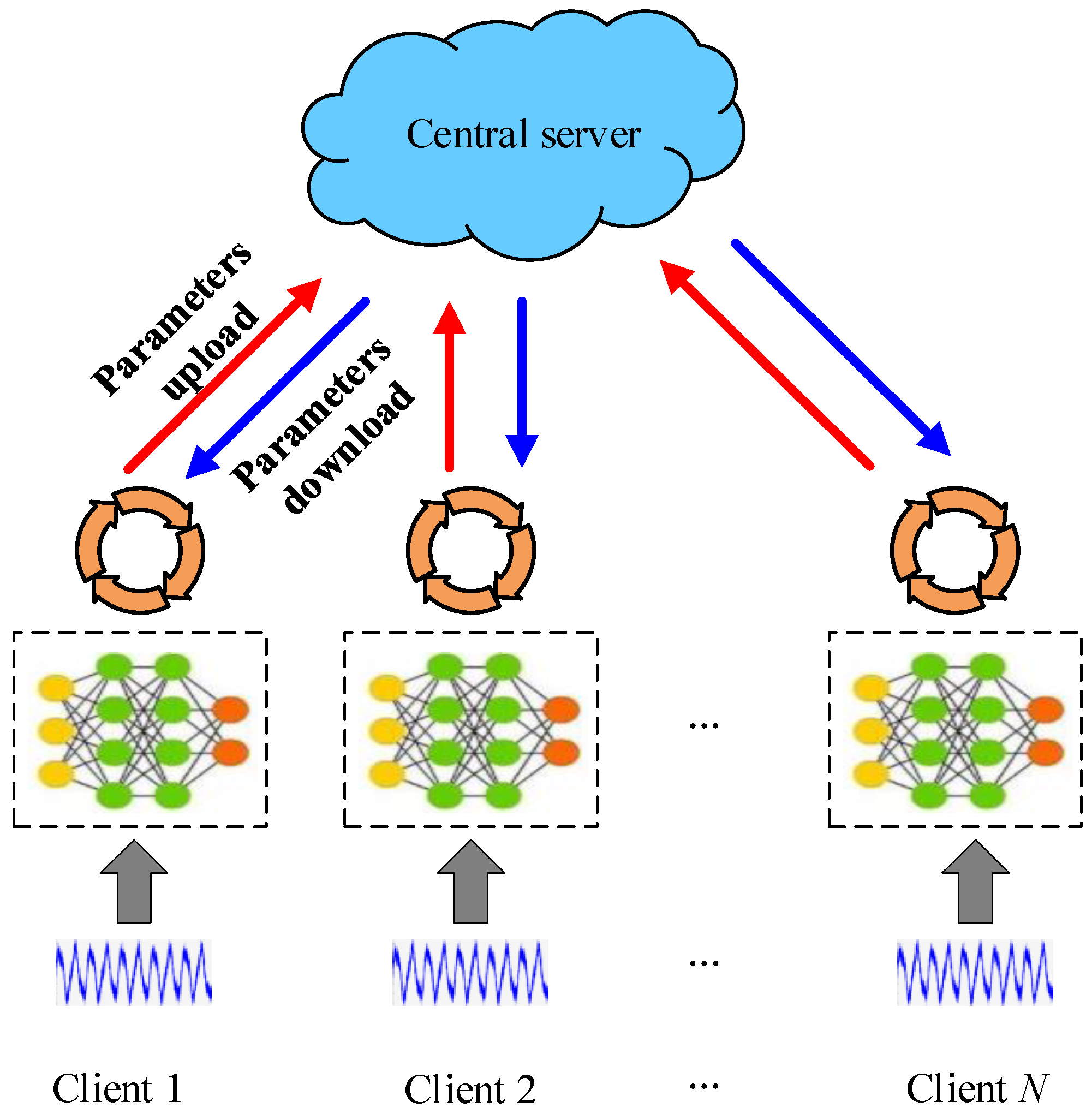
Federated learning is a distributed learning framework that enables multiple clients to collaborate in training a global model, as shown in Figure 1.
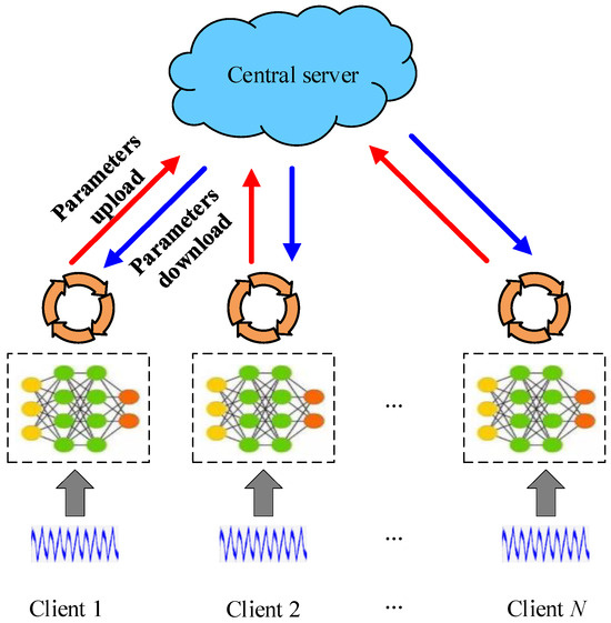
Figure 1.
Basic framework for federal learning.
Federated learning enables privacy and security protection by allowing for clients to train a model collaboratively, without transferring or accessing each other’s raw data. Typically, a central server coordinates the training process. The objective function of the commonly used Federated Averaging algorithm (FedAvg) is as follows:
where represents the loss function of client ; denotes the model parameters being trained; is the aggregate weight of the client, and is generally defined as , where is the sample size of client participating in training, and is the total sample size.
The federated learning training process proposed in this paper consists of the following four steps:
- (1)
- The server selects clients to participate in training and sends them the global model.
- (2)
- The selected clients train locally and update their local model parameters.
- (3)
- The clients upload their updated local model parameters to the server, where indicates the training round.
- (4)
- The server aggregates the uploaded models and updates the global model parameters.
3.2. Variational Auto-Encoding
Variational auto-encoding (VAE), like Generative Adversarial Networks (GANs), can generate data that are similar to the input sample. The basic principle is illustrated in Figure 2.
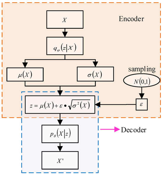
Figure 2.
The basic principle of VAE.
The encoder is used to extract features from the input data, while the generator generates similar tensors with the extracted features. The decoder then reconstructs the input signal. The basic idea is to use latent variable to represent the input data and model the distribution of . By optimizing the encoder parameters , the reconstructed data are made as similar as possible to the input data . Assume that represents the marginal distribution of the reconstructed data.
where represents the probability distribution of the input data reconstructed from the latent variable , while represents the prior distribution of . In this paper, we express using the standard Gaussian distribution .
We expect that the latent variable can generate samples that are similar to the input samples. is used to represent the probability distribution of the latent variable obtained from input data through encoding learning. However, the true is difficult to calculate, so we use a Gaussian distribution with a diagonal covariance structure (where represents the encoder parameter) to approximate the true posterior distribution. The degree of approximation between the two distributions is measured using KL divergence. See the following formula for details:
The above formula represents the expected value of the logarithmic difference between two distributions for . The smaller the value, the higher the similarity between the two distributions.
According to Bayes’ theorem:
By substituting Equation (4) into Equation (3), we can obtain the following:
In Equation (5), we aim to maximize the value of and minimize the value of , so the second term on the right side of Equation (5) must be maximized. Therefore, for the ith sample, we have the following loss function:
As can be seen, the above loss function consists of two parts: the first is the KL divergence between the encoding probability distribution and the prior distribution of the latent variable , and the second is the reconstruction error, similar to an autoencoder. is the encoder with parameter , while is the decoder with parameter .
Suppose ; then
where and are the mean and variance of the approximate posterior distribution, respectively.
Based on the assumption in Equation (7), the KL divergence and reconstruction error in Equation (6) can be expressed more concretely using Equations (8) and (9).
where is the dimension of the latent variable , is the dimension of the input data, and and represent the mean and variance of sample , respectively.
In order to enable backpropagation for the latent variables obtained through random sampling, we use the reparameterization trick to calculate by randomly sampling , where .
Since the output structure of the encoder and decoder is a probability density distribution constrained by model parameters rather than specific eigenvalues, it has better feature representation capabilities. Additionally, due to the presence of random variables, overfitting is less likely to occur, even with small sample sizes and repeated training.
The decision to employ a Variational Auto-Encoder (VAE) architecture in our proposed method is rooted in its unique capabilities, which are well-suited for the challenges inherent in equipment fault diagnosis, particularly in federated learning scenarios.
- (1)
- Feature representation ability: VAEs are adept at learning a deep representation of data through their encoder–decoder structure. The encoder maps input data to a latent space, while the decoder reconstructs the data from this latent representation. This ability is crucial for capturing the nuanced patterns within fault signals, which are often obscured by noise and operational variability.
- (2)
- Handling non-IID data: One of the key challenges in federated learning is the non-independent and identically distributed (non-IID) nature of data across devices. VAEs, through their generative mechanism, can model complex data distributions, allowing our method to effectively handle the heterogeneity in data collected from diverse equipment under varying conditions.
- (3)
- Mitigating overfitting: The introduction of randomness in VAEs, via the stochasticity in the latent space, inherently regularizes the model, reducing the risk of overfitting. This is particularly beneficial when dealing with small sample sizes, as is common in the case of new equipment with limited fault data.
- (4)
- Few-shot learning: The generative nature of VAEs also facilitates few-shot learning, enabling the model to generalize from a small number of examples. This is instrumental for training classifiers in the target domain with a minimal amount of labeled data, thus enhancing the model’s adaptability to new equipment.
- (5)
- Optimization for federated learning: The training procedure involves a customized optimization scheme that includes a regularized federated learning approach for non-IID data. This ensures that the global model benefits from the collective knowledge of the source domains while being fine-tuned to adapt to the specific characteristics of the target domain.
- (6)
- Discriminator for domain consistency: The incorporation of a discriminator in our model further ensures that the features extracted from the source and target domains are aligned, thus maintaining consistency across domains and improving the model’s generalization ability.
4. Proposed Method
4.1. Method Overview
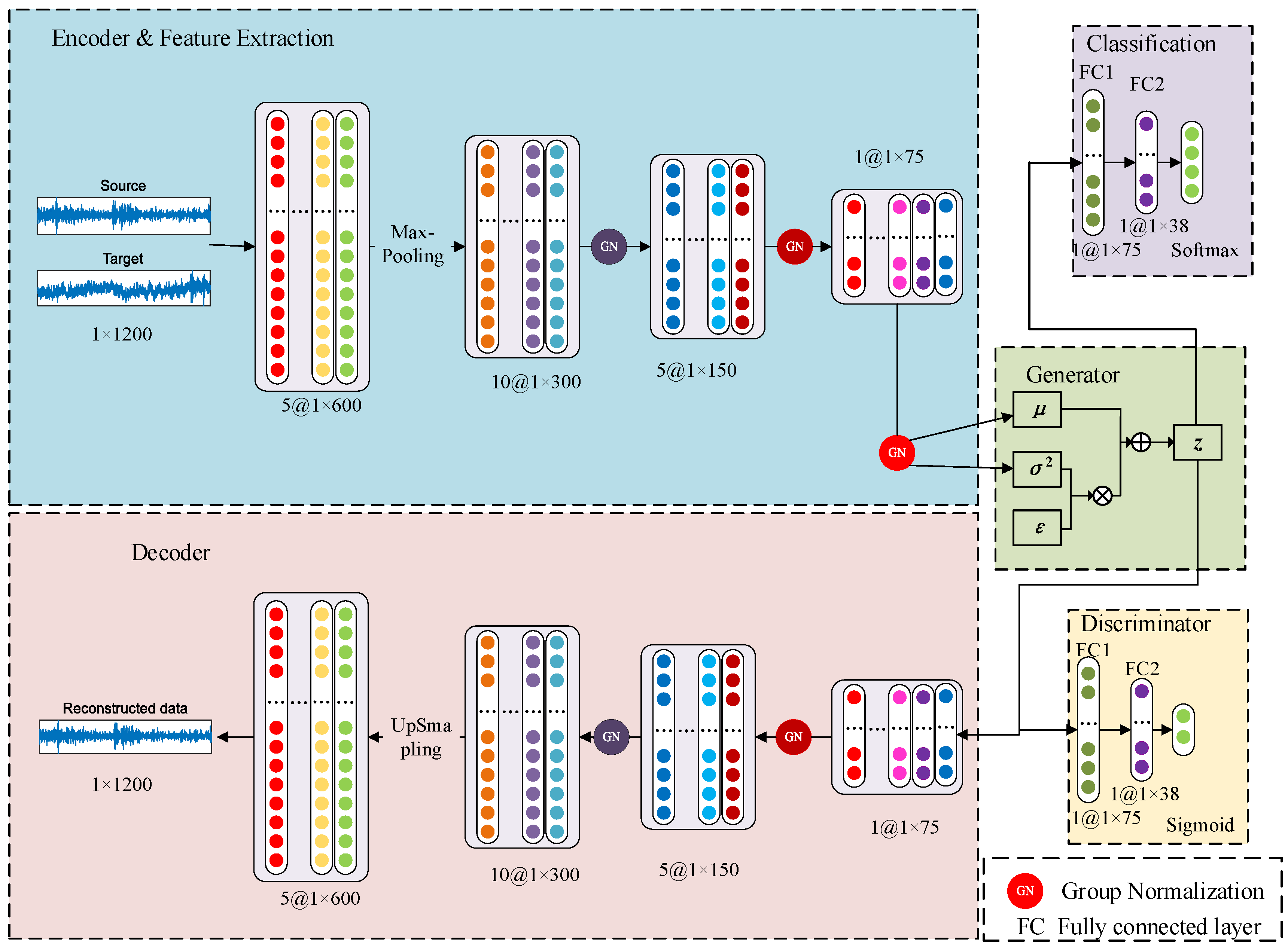
The structure of the global model proposed in this paper is illustrated in Figure 3. The model consists of an encoder (feature extractor), a decoder, a feature generator, a classifier, and a discriminator.
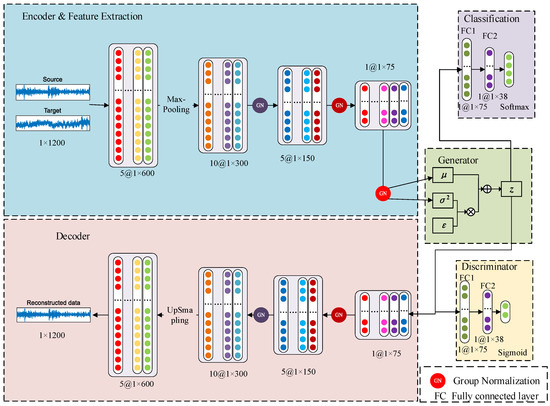
Figure 3.
Federated fault diagnosis model based on variational auto-encoding.
Both the encoder and decoder are composed of four one-dimensional convolutional layers, supplemented by group normalization to accelerate the convergence rate of the model. The feature generator primarily uses variational encoding principles to generate data with the same distribution as that extracted by the feature extractor. After many training iterations, it effectively represents the distribution of features. The classifier is used to distinguish specific fault categories, while the discriminator is used to determine whether the extracted features come from the same distribution space. Both the classifier and discriminator are composed of two fully connected layers, with 75 and 38 neural units, respectively. It should be noted that, in this paper, the decoder is primarily used to constrain the feature generator, specifically through the reconstruction error between generated data and input data, while backpropagation is used to constrain the generator and encoder.
4.2. Optimization Scheme
After a training instruction is issued by the central server, the optimization schemes involved in the training process for both the source and target domains are as follows:
- (1)
- Source domain training process
During the local training process for the source domain, in addition to minimizing the objective Function (6), the classifier should also be as accurate as possible, meaning it should satisfy the objective Function (11).
Equation (11) is the smoothed cross-entropy loss function, which is used in this paper to enhance the model’s generalization ability and reduce overfitting. is the smoothing coefficient, which is set to 0.1 in this paper. represents the number of samples, represents the number of faults, represents the label for the jth category of the ith sample, and represents the predicted probability for the jth category of the ith sample. The first term in the above Equation is the predicted probability for the correct category, while the second term is the average predicted probability for all categories.
To ensure that the features of the source and target domains have similar distributions, it is necessary to train the discriminator’s ability to distinguish between them using binary cross-entropy as the objective function. Let be the output of the discriminator and be the domain label, where for the source domain and for the target domain. The loss function is shown in Equation (12).
where calculates the loss for samples belonging to the positive class, while calculates the loss for samples belonging to the negative class. The negative sign is used to minimize the loss value.
For training samples in the source domain, the total loss function during training can be expressed as follows:
where , and are weight coefficients. After several attempts, the final selected values for these coefficients are , and .
- (2)
- Target domain training process
After all source domain clients complete their local model training, they upload their parameters to the server. The server then generates global model parameters using Formula (1) and sends the aggregated global model to the target client for adaptive domain training. To make the feature distribution extracted from the target domain more similar to that of the source domain, all unlabeled data from the target domain are used in training. During training, the discriminator is fixed and the domain label y is set to 1 to train only the feature extractor and feature generator. The loss function used is .
Next, the global model is fine-tuned using a small number of labeled samples from the target domain. Since the data from the target and source domains belong to a non-independent co-distribution, there are differences in their feature distributions. Using the source domain classifier directly may result in misclassification. Therefore, a new classifier is trained on a small sample at the target client. The structure of this new classifier is the same as that used for training in the source domain. To make it easier to distinguish between different fault categories in the target domain, we aim to maximize the center distance between them. In this paper, we use Euclidean distance to measure the distance between different fault centers in the target domain.
where represents the dimension of the extracted feature and is equal to 75. The symbol represents the mean calculation, while represents the ith feature value of the mth fault.
The new classifier is constrained using the smooth cross-entropy loss function. As a result, the overall loss function during the training process of the labeled small-sample target-domain data is as follows:
where a and b are weight coefficients and the minus sign indicates that the target value is being minimized. After several attempts, the values of and were chosen for the experiment in this paper.
At this stage, all clients, including those in the source and target domains, have completed a full round of training. The target-domain client will upload the optimized global model parameters to the server in preparation for the next round of global training. This process will continue until all training rounds are completed.
4.3. Federated Learning Process
We propose a federated learning framework that utilizes variational coding enhancement. The specific process is outlined below:
Input: central server , labeled fault data from the client , unlabeled fault data, and a small amount of labeled fault data from the target client .
Output: fault category of the target client.
The pseudo-code is as follows:
| // Server-side execution: | |
| 1 | Initialize the global model |
| 2 | do |
| 3 | Receive the model parameters sent by the target domain client and send them to the |
| source domain client participating in the training | |
| // Source domain client parallel training | |
| 4 | Receive the model parameters sent by the server |
| 5 | do |
| 6 | Local model training |
| 7 | end |
| 8 | Upload local model parameters to the server |
| // Server-side execution | |
| 9 | Aggregation forms a global model |
| 10 | Deliver the global model to the target domain client |
| // Execute on the target domain client | |
| 11 | do |
| 12 | Sample field adaptive training without labels |
| 13 | Small sample fine tuning training with labels |
| 14 | end |
| 15 | Upload the trained model parameters to the server |
| 16 | end |
| // Target domain sample prediction | |
| 17 | The test samples are fed into the trained feature extractor and new classifier for fault classification. |
5. Experiment
5.1. Experiment on Cross-Working Conditions
- (1)
- Experimental overview
The experimental data were obtained from the public dataset of the Spectra Quest (SQ) experiment platform at Xi’an Jiaotong University [25]. The test stand used is shown in Figure 4. The bearing model used in the experiment was the NSK Company’s 6203 bearing. The dataset simulates three failure modes: normal motor bearing, outer ring failure, and inner ring failure. Motor-bearing vibration signals were collected for three different degrees of fault (mild, moderate, and severe) at three rotation frequencies (19.05 Hz, 29.05 Hz, and 39.05 Hz). A piezoelectric acceleration sensor was used to collect motor bearing signals during the experiment. The data acquisition instrument model was CoCo80, with a sampling frequency of 25.6 KHz and an acceleration sensor sensitivity of 50 mv/g.

Figure 4.
Bearing data test stand of Spectra Quest.
In this paper, the source domain data were selected from data with a rotation frequency of 29.05 Hz, while the target-domain data were selected from data with a rotation frequency of 39.05 Hz. Furthermore, each client in this study possesses only one labeled fault datum with varying degrees, as presented in Table 1. The samples in the table were generated using the sliding window method, with each sample comprising 1200 data points. Specifically, the samples were taken at intervals of 600 points.

Table 1.
Attributes of cross-working condition experimental data.
Clearly, the rotational frequency of the source domain client differs from that of the target-domain client, indicating that their working conditions are different. Additionally, each client in the source domain has only one calibrated fault category sample. In reality, the fault categories of a device are generally limited. In this paper, we use an extreme case where a source domain client has only one fault sample to test the performance of our proposed method.
- (2)
- Experimental settingTo verify the effectiveness of the proposed method, we use several common methods for simultaneous training and prediction.
- (a)
- VAE-FedAvg (proposed method): Training and recognition are conducted according to the structure shown in Figure 3 and the process described in Section 4.3. During local training on the source domain client, the batch size is set to 32 and the number of local training iterations is set to 30. When the target client uses a small number of labeled samples to fine-tune the global model, 60 training iterations are set.
- (b)
- Baseline: Each source domain client conducts training independently, once. After training is completed, the local model parameters are uploaded to the server. The server then collects all client model parameters and uses an averaging algorithm for model aggregation before sending the aggregated model parameters to the target client. The target client uses the labeled small-sample data to fine-tune the training model. Then, other target-domain sample data are identified. The structure of the model uses the same encoder (feature extraction) and classifier as shown in Figure 3.
- (c)
- Centralized: All client data are centralized for training. The framework consists of the encoder and classifier shown in Figure 3. It should be noted that this method does not provide privacy protection.
- (d)
- VAE-without source: Without source domain data, only a small amount of labeled target-domain sample data are used for model training. The model used consists of the encoder, decoder, generator, and classifier shown in Figure 3.
- (3)
- Experimental results and analysis
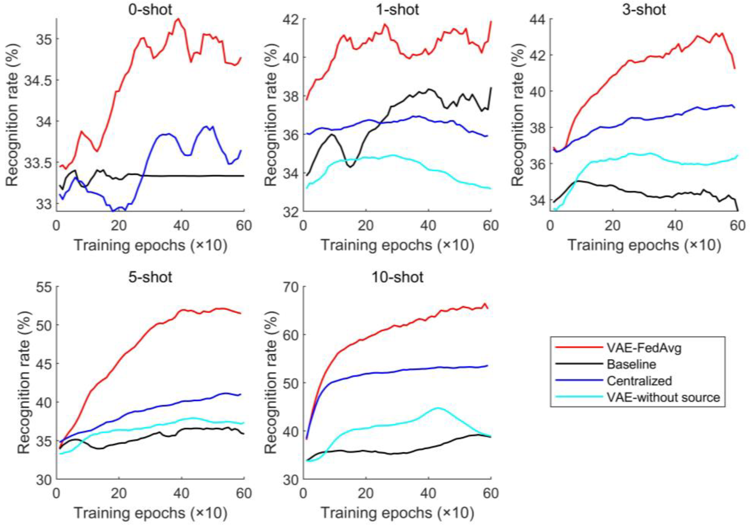
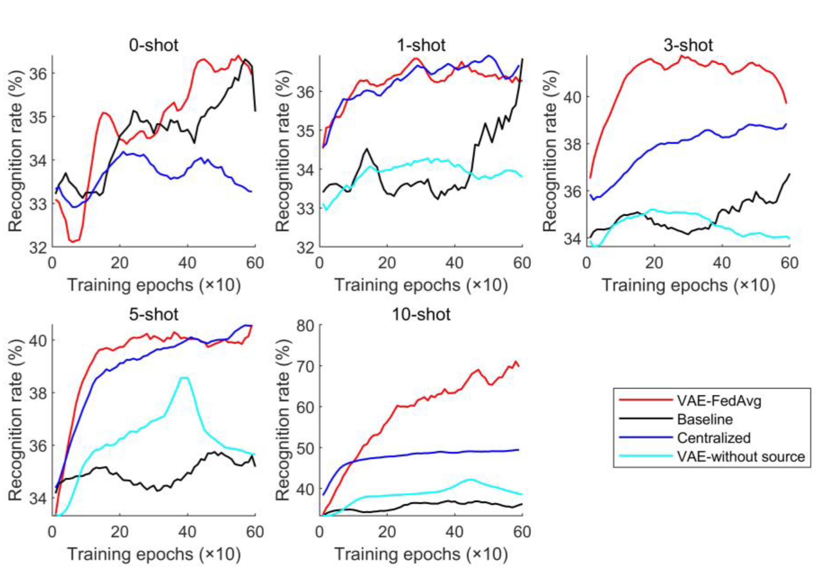
The number of training epochs was set to 600, the learning rate for each module was set to 0.001, and the batch size was 32. To simulate the scarcity of labeled samples in engineering practice, 0, 1, 3, 5, and 10 samples of each fault category in the target domain were selected as fine-tuning samples. These fine-tuning samples were not used as target samples for prediction. To reduce the influence of randomly initialized model parameters on model prediction performance, the above four methods were repeated 10 times. The average recognition rate was calculated and its changes over the training epochs were plotted as a curve graph, shown in Figure 5.
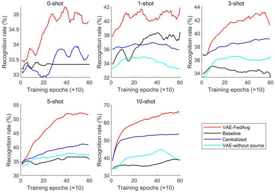
Figure 5.
Prediction results under cross-working conditions.
As seen from the prediction results in Figure 5, our proposed method has clear advantages over other methods. Even without fine-tuning samples (0-shot), our method still presents with a good recognition performance, indicating that VAE has an excellent feature extraction ability. As the number of fine-tuning samples increases, prediction performance and stability improve. Generally speaking, the centralized training method often has the best performance, but it lacks the generating module (i.e., the VAE module) in the network structure, so their performance is not as good as that of our method.
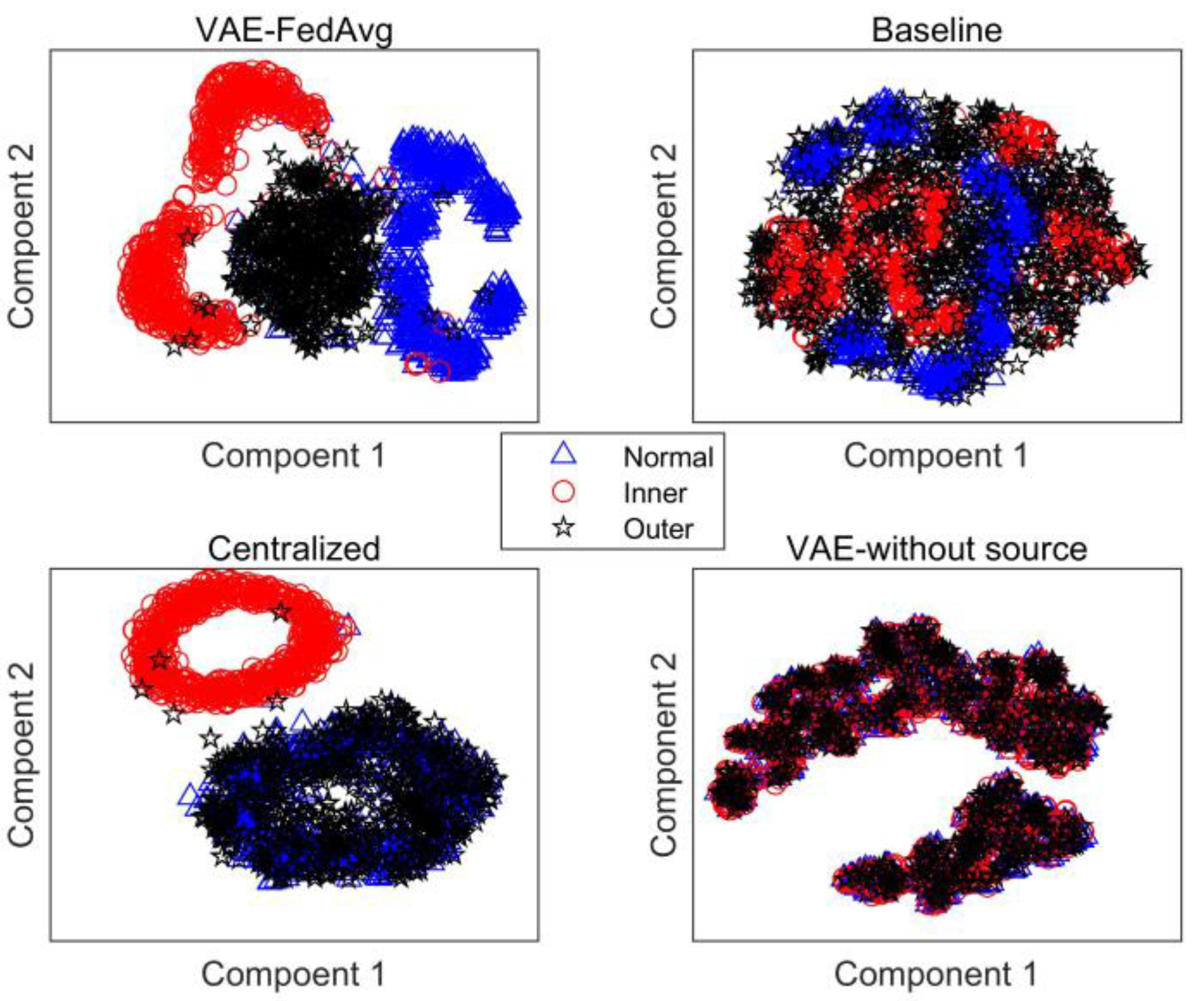
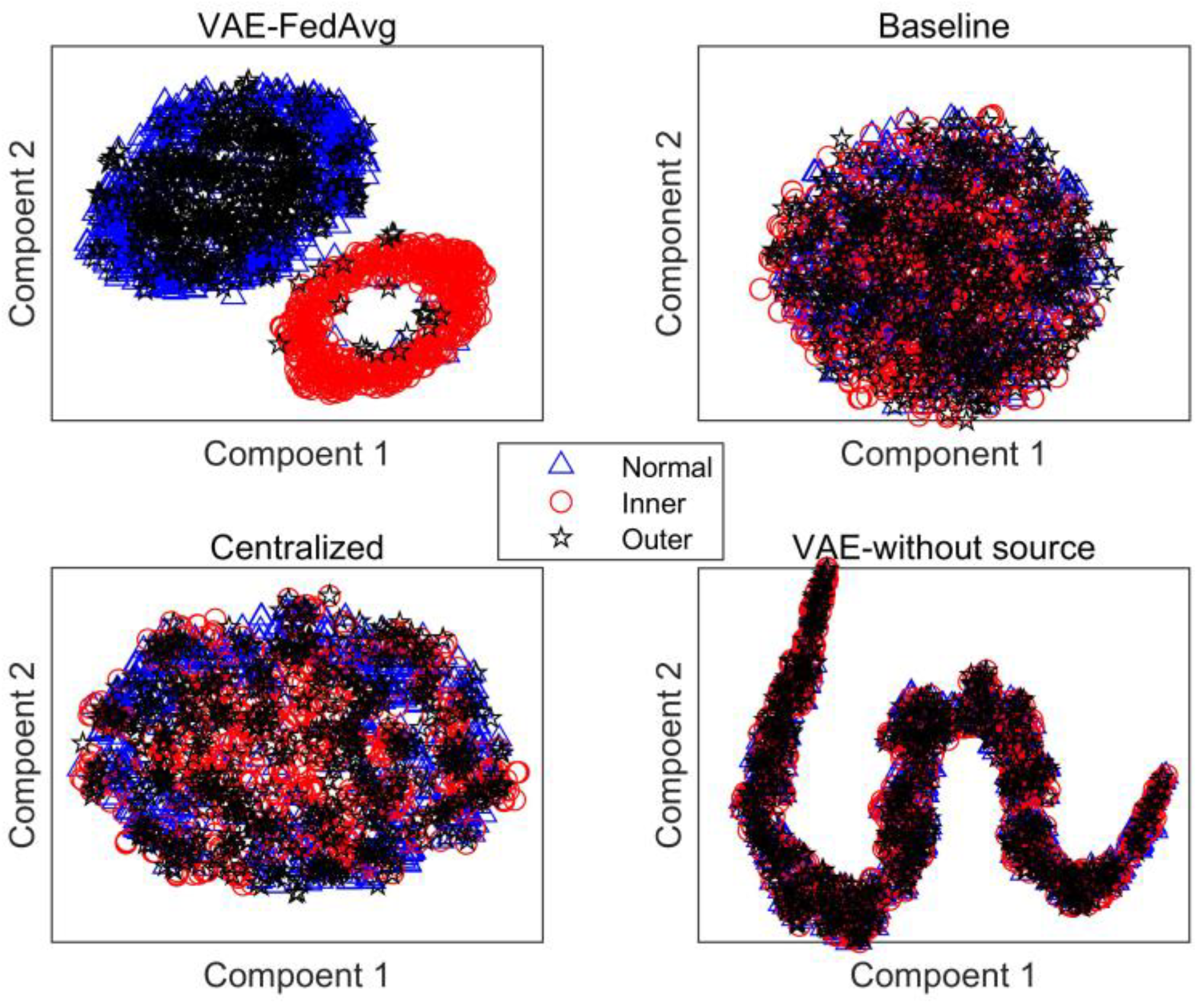
The main reason why VAE can improve the model’s recognition rate is that it can further obtain the distribution of features based on feature extraction and generate simulated features with the same distribution as the extracted features. This helps to solve the problem of model overfitting due to a small number of samples. In this paper, we also attempt to identify the target domain using VAE and training with only a few labeled samples. As seen in Figure 5, the results are not ideal but are similar to the baseline method. This is because a small number of samples cannot accurately represent the true distribution of features. Our proposed method trains the model with a large number of samples in the source domain to improve its feature extraction ability. Then, a small number of target-domain labeled samples are used to fine-tune the trained model, ensuring its performance and adaptation to the distribution of target-domain samples. To further demonstrate the advantages of our proposed method in feature extraction, we use 10 fine-tuning samples for each fault as an example. The features extracted by the four methods were reduced to two dimensions using the t-distribution neighborhood embedding algorithm and plotted as a planar graph, shown in Figure 6. The recognition results for each type of fault were plotted as a confusion matrix, shown in Figure 7.

Figure 6.
Feature distribution under cross-working conditions.

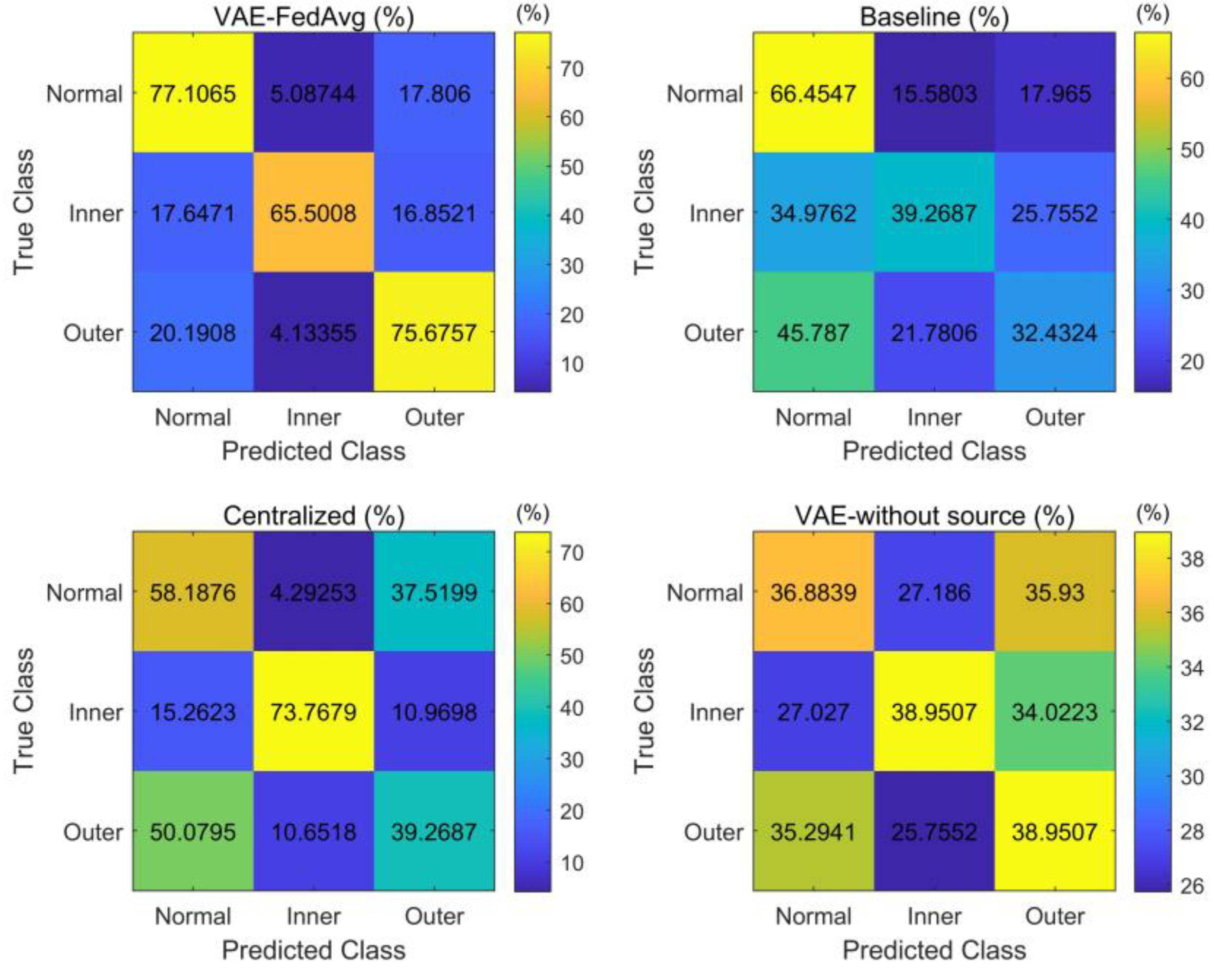
Figure 7.
Confusion matrix of recognition results under cross-working conditions.
As seen in Figure 6, the three fault features extracted by our proposed method are well-differentiated, while the features extracted by the other methods overlap significantly. This is also confirmed by their recognition rates.
As seen in Figure 7, our proposed method is relatively balanced in identifying the three types of faults, while other methods have high recognition rates only for individual fault types and poor balance. This demonstrates that our proposed method can effectively capture the features of various faults even with a small number of samples.
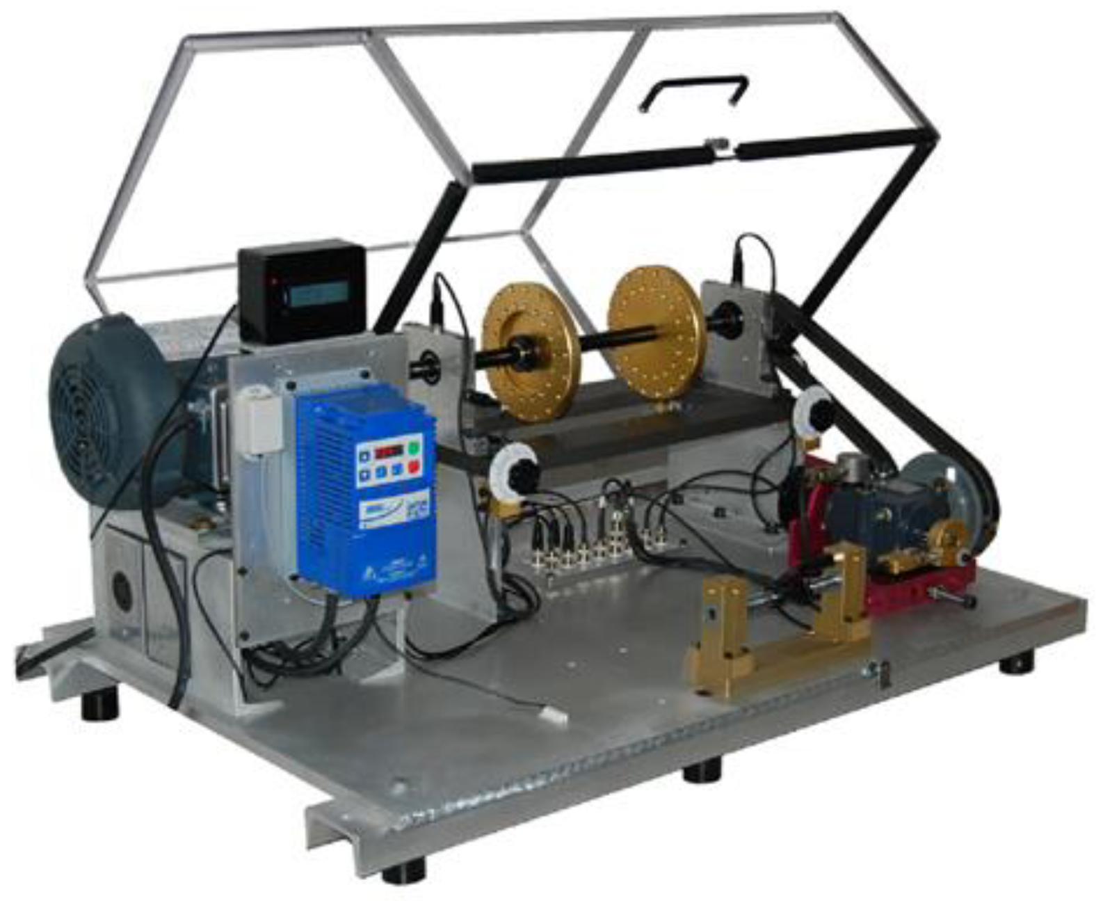
5.2. Experiment on Cross-Device
The source domain data for the experiment came from the bearing dataset of Paderborn University in Germany [35], and the test stand that was used is shown in Figure 8. The experimental bearing was also the 6203 bearing, and the vibration signal of the bearing seat was collected by a piezoelectric accelerometer with a sampling frequency of 64 kHz. Experiments were conducted under different load torques, rotational speeds, and radial forces. In this paper, we selected experimental data from three conditions, as shown in Table 2.
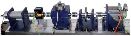
Figure 8.
Bearing data test stand of Paderborn University.
Table 2.
Attributes of experimental source domain data across devices.
To verify the cross-device transfer effect of our proposed method, the target-domain client still used the target-domain data in Table 1. The parameter settings were the same as in Section 5.1. The experimental recognition results are shown in Figure 9.
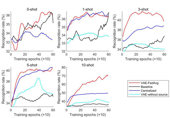
Figure 9.
Prediction results under cross-devices.
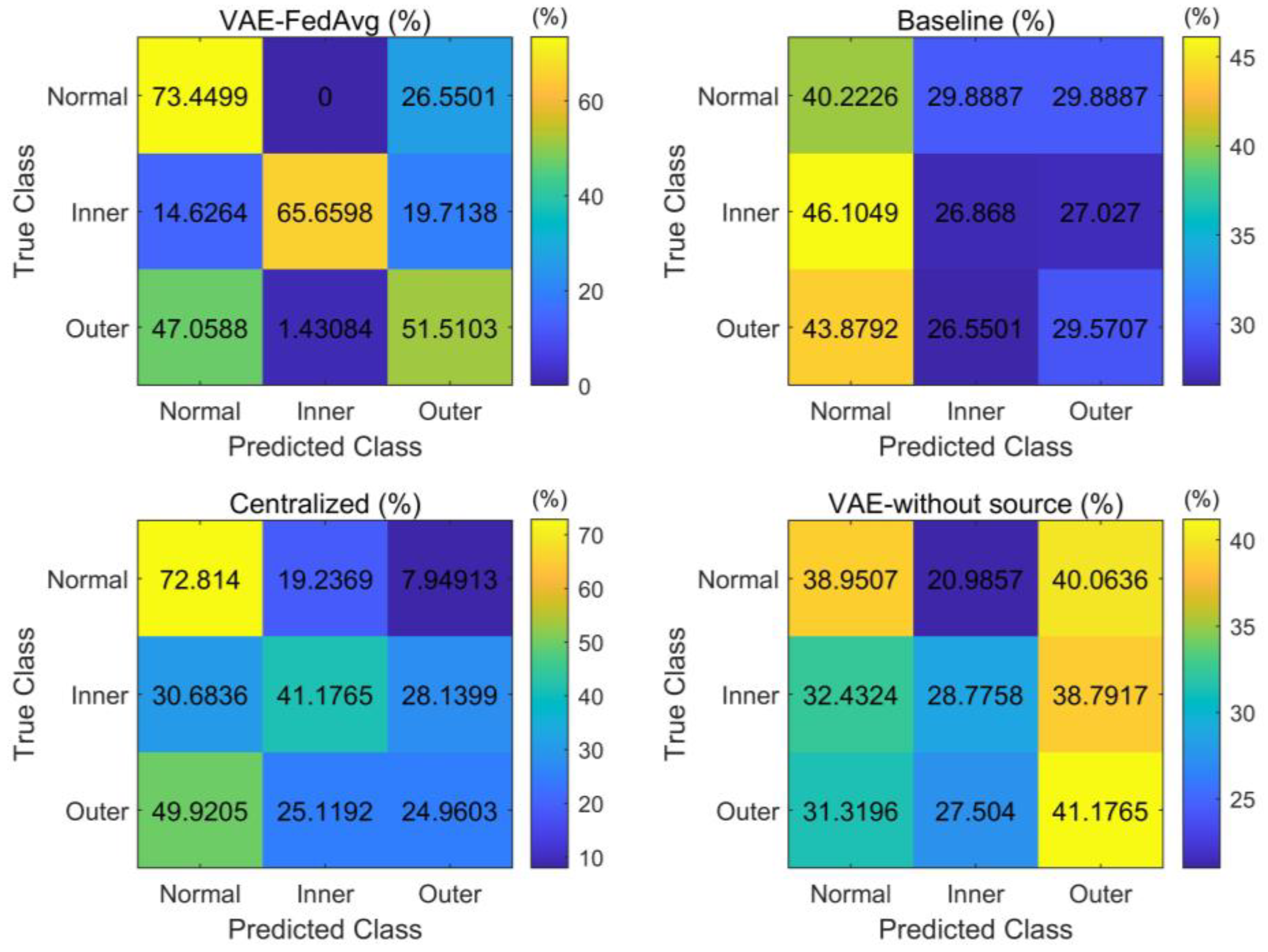
Although the bearing models in both the source and target domains are identical, they are installed on different devices and operate under varying loads, speeds, frequencies, and acquisition sensors. As shown in Figure 9, our proposed method can still achieve good recognition results when applied to cross-device transfer learning. For instance, when we take 10 fine-tuned labeled samples and use the t-distribution neighborhood embedding algorithm to plot their extracted features onto a two-dimensional plane (as shown in Figure 10), we can see that the identification results for each fault in the target domain are clearly displayed in a confusion matrix (as shown in Figure 11).

Figure 10.
The distribution of the extracted features under cross-device.
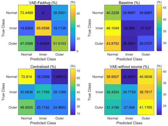
Figure 11.
The confusion matrix of recognition results under the cross-device.
6. Conclusions
This article presents a novel approach to mechanical fault diagnosis in federated learning based on VAE. It provides a new solution for cross-domain and even cross-device federated transfer fault diagnosis, enabling the distributed training, fine-tuning, and transfer application of intelligent diagnostic models while ensuring data privacy.
- (1)
- A cross-domain transfer learning framework based on federated learning is established, taking into account the requirements for data privacy protection. Without the need for raw data transmission, the model’s feature extraction capability is adaptively adjusted according to different working conditions, facilitating the extraction of effective features across domains.
- (2)
- A feature distribution extraction method based on VAE is proposed, addressing the challenge of extracting effective features under non-independent and non-identically distributed conditions. The stochastic generation function of VAE also helps to mitigate overfitting during training.
- (3)
- A federated learning fine-tuning method with a small number of samples is introduced. In cross-working conditions or cross-device scenarios, a limited number of labeled target-domain samples are involved in training the federated global model. This allows the global model to learn the feature distribution patterns of the target domain while benefiting from the recognition experience of the source domain, thereby enhancing its recognition capability regarding the target.
The results of the two experiments demonstrate that the proposed method outperforms other transfer methods in terms of recognition accuracy, while preserving data privacy. By leveraging a small number of labeled samples to fine-tune the federated training model, this approach achieves a superior performance across various working conditions and even in cross-device scenarios.
Author Contributions
Writing—review & editing, Y.R.; Funding acquisition, Y.G. All authors have read and agreed to the published version of the manuscript.
Funding
This work was supported in part by the Suzhou Science and Technology Foundation of China under Grant SYG202021, Jiangsu Provincial Natural Science Research Foundation of China under Grant 21KJA510003, Jiangsu Key Laboratory for Elevator Intelligent Safety under Grant JSKLESS202101.
Data Availability Statement
The data presented in this study are available on request from the corresponding author.
Conflicts of Interest
The authors declared that they have no conflicts of interest in this work.
References
- Chen, Z.; Gryllias, K.; Li, W. Intelligent Fault Diagnosis for Rotary Machinery Using Transferable Convolutional Neural Network. IEEE Trans. Ind. Inform. 2020, 16, 339–349. [Google Scholar] [CrossRef]
- Qian, C.; Zhu, J.; Shen, Y.; Jiang, Q.; Zhang, Q. Deep Transfer Learning in Mechanical Intelligent Fault Diagnosis: Application and Challenge. Neural Process. Lett. 2022, 54, 2509–2531. [Google Scholar] [CrossRef]
- Xiong, X.; Jiang, H.K.; Li, X.; Niu, M. A Wasserstein gradient-penalty generative adversarial network with deep auto-encoder for bearing intelligent fault diagnosis. Meas. Sci. Technol. 2020, 31, 045006. [Google Scholar] [CrossRef]
- Elbir, A.M.; Coleri, S.; Papazafeiropoulos, A.K.; Kourtessis, P.; Chatzinotas, S. A Hybrid Architecture for Federated and Centralized Learning. IEEE Trans. Cogn. Commun. Netw. 2022, 8, 1529–1542. [Google Scholar] [CrossRef]
- Chen, J.; Li, J.; Huang, R.; Yue, K.; Chen, Z.; Li, W. Federated Transfer Learning for Bearing Fault Diagnosis with Discrepancy-Based Weighted Federated Averaging. IEEE Trans. Instrum. Meas. 2022, 71, 1–11. [Google Scholar] [CrossRef]
- Li, Z.; Li, Z.; Li, Y.; Tao, J.; Mao, Q.; Zhang, X. An Intelligent Diagnosis Method for Machine Fault Based on Federated Learning. Appl. Sci. 2021, 11, 12117. [Google Scholar] [CrossRef]
- Wang, S.; Zhang, Y. Multi-Level Federated Network Based on Interpretable Indicators for Ship Rolling Bearing Fault Diagnosis. J. Mar. Sci. Eng. 2022, 10, 743. [Google Scholar] [CrossRef]
- Mohammadabadi, S.M.S.; Liu, Y.; Canafe, A.; Yang, L. Towards Distributed Learning of PMU Data: A Federated Learning based Event Classification Approach. In Proceedings of the Conference Towards Distributed Learning of PMU Data: A Federated Learning Based Event Classification Approach, IEEE Computer Society, Orlando, FL, USA, 16–20 July 2023. [Google Scholar]
- Hou, S.; Lu, J.; Zhu, E.; Zhang, H.; Ye, A. A Federated Learning-Based Fault Detection Algorithm for Power Terminals. Math. Probl. Eng. 2022, 2022, 1–10. [Google Scholar] [CrossRef]
- Zhang, W.; Wang, Z.; Li, X. Blockchain-based decentralized federated transfer learning methodology for collaborative machinery fault diagnosis. Reliab. Eng. Syst. Saf. 2023, 229, 108885. [Google Scholar] [CrossRef]
- Zhang, X.; Ma, Z.; Wang, A.; Mi, H.; Hang, J. LstFcFedLear: A LSTM-FC with Vertical Federated Learning Network for Fault Prediction. Wirel. Commun. Mob. Comput. 2021, 2021, 2668761. [Google Scholar] [CrossRef]
- Cui, L.; Qu, Y.; Xie, G.; Zeng, D.; Li, R.; Shen, S.; Yu, S. Security and Privacy-Enhanced Federated Learning for Anomaly Detection in IoT Infrastructures. IEEE Trans. Ind. Inform. 2022, 18, 3492–3500. [Google Scholar] [CrossRef]
- Massaoudi, M.; Abu-Rub, H.; Refaat, S.S.; Chihi, I.; Oueslati, F.S. Deep Learning in Smart Grid Technology: A Review of Recent Advancements and Future Prospects. IEEE Access 2021, 9, 54558–54578. [Google Scholar] [CrossRef]
- Du, J.; Qin, N.; Huang, D.; Zhang, Y.; Jia, X. An Efficient Federated Learning Framework for Machinery Fault Diagnosis with Improved Model Aggregation and Local Model Training. IEEE Trans. Neural Netw. Learn. Syst. 2023, 35, 10086–10097. [Google Scholar] [CrossRef] [PubMed]
- Ma, X.; Wen, C.L. An Asynchronous Quasi-Cloud/Edge/Client Collaborative Federated Learning Mechanism for Fault Diagnosis. Chin. J. Electron. 2021, 30, 969–977. [Google Scholar]
- Huo, C.; Jiang, Q.; Shen, Y.; Zhu, Q.; Zhang, Q. Enhanced transfer learning method for rolling bearing fault diagnosis based on linear superposition network. Eng. Appl. Artif. Intell. 2023, 121, 105970. [Google Scholar] [CrossRef]
- Zhang, Q.; He, Q.; Qin, J.; Duan, J. Application of Fault Diagnosis Method Combining Finite Element Method and Transfer Learning for Insufficient Turbine Rotor Fault Samples. Entropy 2023, 25, 414. [Google Scholar] [CrossRef] [PubMed]
- Li, S.; Yu, J. A Multisource Domain Adaptation Network for Process Fault Diagnosis Under Different Working Conditions. IEEE Trans. Ind. Electron. 2023, 70, 6272–6283. [Google Scholar] [CrossRef]
- Ma, Y.; Liu, Y.; Yang, Z.; Cheng, M.; Meng, H. Deep adversarial transfer neural network for fault diagnosis of wind turbine gearbox. Int. J. Green Energy 2023, 20, 1750–1762. [Google Scholar] [CrossRef]
- Wang, Y.; Ge, L.; Xue, C.; Li, X.; Meng, X.; Ding, X. Multiple local domains transfer network for equipment fault intelligent identification. Eng. Appl. Artif. Intell. 2023, 120, 105791. [Google Scholar] [CrossRef]
- Peng, R.; Zhang, X.; Shi, P. Multi-Representation Domain Adaptation Network with Duplex Adversarial Learning for Hot-Rolling Mill Fault Diagnosis. Entropy 2023, 25, 83. [Google Scholar] [CrossRef]
- Liu, G.; Shen, W.; Gao, L.; Kusiak, A. Active Broad-Transfer Learning Algorithm for Class-Imbalanced Fault Diagnosis. IEEE Trans. Instrum. Meas. 2022, 72, 1–16. [Google Scholar] [CrossRef]
- Ma, W.; Liu, R.; Guo, J.; Wang, Z.; Ma, L. A collaborative central domain adaptation approach with multi-order graph embedding for bearing fault diagnosis under few-shot samples. Appl. Soft Comput. 2023, 140, 110243. [Google Scholar] [CrossRef]
- Wang, H.; Xu, Z.; Tong, X.; Song, L. Cross-Domain Open Set Fault Diagnosis Based on Weighted Domain Adaptation with Double Classifiers. Sensors 2023, 23, 2137. [Google Scholar] [CrossRef] [PubMed]
- Geng, D.; He, H.; Lan, X.; Liu, C. Bearing fault diagnosis based on improved federated learning algorithm. Computing 2022, 104, 1–19. [Google Scholar] [CrossRef]
- Yang, W.; Yu, G. Federated Multi-Model Transfer Learning-Based Fault Diagnosis with Peer-to-Peer Network for Wind Turbine Cluster. Machines 2022, 10, 972. [Google Scholar] [CrossRef]
- Zhang, J.; Zhang, K.; An, Y.; Luo, H.; Yin, S. An Integrated Multitasking Intelligent Bearing Fault Diagnosis Scheme Based on Representation Learning Under Imbalanced Sample Condition. IEEE Trans. Neural Netw. Learn. Syst. 2023, 35, 6231–6242. [Google Scholar] [CrossRef] [PubMed]
- Zhang, W.; Li, X. Data privacy preserving federated transfer learning in machinery fault diagnostics using prior distributions. Struct. Health Monit. Int. J. 2022, 21, 1329–1344. [Google Scholar] [CrossRef]
- Zhang, W.; Li, X. Federated Transfer Learning for Intelligent Fault Diagnostics Using Deep Adversarial Networks with Data Privacy. IEEE/ASME Trans. Mechatron. 2021, 27, 430–439. [Google Scholar] [CrossRef]
- Liu, Q.; Yang, B.; Wang, Z.; Zhu, D.; Wang, X.; Ma, K.; Guan, X. Asynchronous Decentralized Federated Learning for Collaborative Fault Diagnosis of PV Stations. IEEE Trans. Netw. Sci. Eng. 2022, 9, 1680–1696. [Google Scholar] [CrossRef]
- Li, W.; Yang, W.; Jin, G.; Chen, J.; Li, J.; Huang, R.; Chen, Z. Clustering Federated Learning for Bearing Fault Diagnosis in Aerospace Applications with a Self-Attention Mechanism. Aerospace 2022, 9, 516. [Google Scholar] [CrossRef]
- Modirrousta, M.H.; Shoorehdeli, M.A.; Yari, M.; Ghahremani, A. Imbalanced Classification in Faulty Turbine Data: New Proximal Policy Optimization. arXiv 2023, arXiv:2301.04049. [Google Scholar]
- Prybylo, M.; Haghighi, S.; Peddinti, S.T.; Ghanavati, S. Evaluating Privacy Perceptions, Experience, and Behavior of Software Development Teams. arXiv 2024, arXiv:2404.01283. [Google Scholar]
- Nabavirazavi, S.; Taheri, R.; Iyengar, S.S. Enhancing federated learning robustness through randomization and mixture. Future Gener. Comput. Syst. 2024, 158, 28–43. [Google Scholar] [CrossRef]
- Ruan, D.; Wang, J.; Yan, J.; Gühmann, C. CNN parameter design based on fault signal analysis and its application in bearing fault diagnosis. Adv. Eng. Inform. 2023, 55, 101877. [Google Scholar] [CrossRef]


Disclaimer/Publisher’s Note: The statements, opinions and data contained in all publications are solely those of the individual author(s) and contributor(s) and not of MDPI and/or the editor(s). MDPI and/or the editor(s) disclaim responsibility for any injury to people or property resulting from any ideas, methods, instructions or products referred to in the content. |
© 2024 by the authors. Licensee MDPI, Basel, Switzerland. This article is an open access article distributed under the terms and conditions of the Creative Commons Attribution (CC BY) license (https://creativecommons.org/licenses/by/4.0/).