Dynamical Behaviors of a Stochastic Susceptible-Infected-Treated-Recovered-Susceptible Cholera Model with Ornstein-Uhlenbeck Process

Abstract

In this study, a cholera infection model with a bilinear infection rate is developed by considering the perturbation of the infection rate by the mean-reverting process. First of all, we give the existence of a globally unique positive solution for a stochastic system at an arbitrary initial value. On this basis, the sufficient condition for the model to have an ergodic stationary distribution is given by constructing proper Lyapunov functions and tight sets. This indicates in a biological sense the long-term persistence of cholera infection. Furthermore, after transforming the stochastic model to a relevant linearized system, an accurate expression for the probability density function of the stochastic model around a quasi-endemic equilibrium is derived. Subsequently, the sufficient condition to make the disease extinct is also derived. Eventually, the theoretical findings are shown by numerical simulations. Numerical simulations show the impact of regression speed and fluctuation intensity on stochastic systems.

1. Introduction

Infectious diseases have always been an important issue in the field of global public health, with far-reaching impacts on the health of human societies, social order and economic stability. WHO has been actively promoting in-depth research on infectious diseases with the aim of understanding the mechanisms of their occurrence, transmission and control, so as to provide a scientific basis for global health security [1,2,3]. Infectious diseases are diseases caused by pathogens that spread among populations, including viruses, bacteria, parasites and fungi. These pathogens can be transmitted through different routes, such as airborne droplets and bloodborne, foodborne and waterborne transmission, making the control and prevention of infectious diseases extremely complex. One of the typical diseases transmitted from water sources is cholera [4].

Cholera is an infectious disease brought on by infection with the bacterium Vibrio cholerae [5]. Typical symptoms of Vibrio cholerae infection: after infection, it usually leads to the damage of autoimmune cells, which may cause the patient to have a moderate or high fever, and if it is more serious, it may lead to coma or shock. Cholera can be transmitted by a variety of means, including waterborne, foodborne, contact and mosquito transmission [6]. Moreover, cholera patients and carriers are usually the major transmission sources. This article combines the randomness of infectious diseases and focuses on the study of human-to-human contact transmission.

The spread of infectious diseases is a complex process that is influenced by various factors, such as population density, population mobility and pathogen characteristics. Mathematical models can take these factors into account and describe the dynamics of infectious disease transmission by establishing a series of equations [7]. By solving and simulating these equations, scientists can better understand the laws of infectious disease transmission and develop more effective prevention and control strategies [8,9,10,11,12,13]. For instance, Wang et al. [14] proposed a model for spreading cholera epidemics with chronological age and infection age structures. Jiang et al. [15] constructed a diffusion cholera model with non-flux boundary conditions for seasonally forced endowment latency and bacterial hyperinfectivity.

In [16], Tilahun et al. researched a deterministic SITRS mathematical model for cholera by considering the direct contact transmission route as follows:

$$\left\{\begin{array}{cc}\hfill \frac{\mathrm{d}S}{\mathrm{d}t}=& A+pR-\xi S-\beta IS,\hfill \\ \hfill \frac{\mathrm{d}I}{\mathrm{d}t}=& \beta IS-(\xi +d+\sigma )I,\hfill \\ \hfill \frac{\mathrm{d}T}{\mathrm{d}t}=& \sigma I-(\xi +\gamma +g)T,\hfill \\ \hfill \frac{\mathrm{d}R}{\mathrm{d}t}=& \gamma T-(\xi +p)R.\hfill \end{array}\right.$$

(1)

where $S,I,T$ and R stand for susceptible, infected, treated and recovered populations, respectively. A is susceptible to this recruitment rate, $\beta$ is the rate of contact between vulnerable and infected persons, p is the rate of immune loss among recovered individuals, $\xi$ is the natural lethality rate, d is the disease lethality among infected persons, $\sigma$ is the treatment rate among infected individuals, $\gamma$ is the rate of recovery among treated individuals and g is the disease lethality among treated individuals.

There are several conclusions for model (1) as follows:

(1) The number of basic regeneration is $R_0=\frac{\beta A}{\xi (\xi +d+\sigma )}$.

(2) The disease-free equilibrium point $E_0=(S_0,I_0,T_0,R_0)=(\frac{A}{\xi },0,0,0)$ of the system is global asymptotically stable for $R_0<1$. The endemic equilibrium point $E^{*}=(S^{*},I^{*},T^{*},R^{*})$ of the system is local asymptotically stable for $R_0>1$, where

$$S^{*}=\frac{\xi +d+\sigma }{\beta },I^{*}=\frac{\xi +\gamma +g}{\sigma }{T}^{*},R^{*}=\frac{\gamma }{\xi +p}{T}^{*},$$

$$T^{*}=\frac{\sigma (\xi +p)(\beta A-\xi (\xi +d+\sigma \left)\right)}{\beta (\xi +p)(\xi +\gamma +g)(\xi +d+\sigma )-\beta \sigma p\gamma }.$$

Additionally, the presence of random noise in ecosystems can also have an impact on population systems. Therefore, random infectious models with environmental noise can more accurately reflect actual phenomena compared with traditional deterministic infectious disease models [17,18,19,20,21]. To simulate the influence of random noise on contact rate $\beta$, two techniques have been described by Zhang et al. [22]. One way is to use white Gaussian noise to interfere with parameter $\beta$. Another approach is to use the mean-reverting process to interfere with parameter $\beta$.

(1) In the first case,

$$\beta \left(t\right)=\beta +\theta \mathrm{d}B\left(t\right).$$

$B\left(t\right)$ is denoted as standard Brownian movement; $\theta$ is the intensity of white noise. Integrating the above equation and dividing by t gives

$$\frac{1}{t}{\int }_0^t\beta \left(s\right)\mathrm{d}s=\beta +\theta \frac{B\left(t\right)}{t}\sim \mathbb{N}(\beta ,\frac{{\theta }^2}{t})$$

This indicates that when t approaches 0, $\mathbb{V}ar\left[\beta \right(t\left)\right]$ will reach infinity, meaning that $\beta$ fluctuates greatly. This has resulted in very unreasonable results. In [23], Allen’s research shows that compared to linear functions with white Gaussian noise, the mean-reverting process is better able to demonstrate environmental diversity.

In the second case,

$$\mathrm{d}\beta \left(t\right)=k(\beta -\beta (t\left)\right)\mathrm{d}t+\theta \mathrm{d}B\left(t\right),$$

(2)

where $k,\theta$ is a normal number. k is the regression speed, and $\theta$ is the fluctuation intensity. For the above equation, let $m\left(t\right)=\beta \left(t\right)-\beta$ to obtain

$$\mathrm{d}m\left(t\right)=-km\left(t\right)\mathrm{d}t+\theta \mathrm{d}B\left(t\right).$$

By calculation, it is possible to obtain $\mathbb{E}\left[m\left(t\right)\right]=m_0{e}^{-kt},\mathbb{V}ar\left[m\left(t\right)\right]=\frac{{\theta }^2}{2k}(1-e^{-2kt})$ where $m_0:=m\left(0\right)$. Unlike white noise, as $t\to 0$, $\mathbb{V}ar\left[\beta \right(t\left)\right]$ tends towards 0. However, it is easy to have $m\left(t\right)$, being ergodic, weakly converging to an invariant density

$$\zeta \left(x\right)=\frac{\sqrt{k}}{\sqrt{\pi }\theta }{e}^{-\frac{k{x}^2}{{\theta }^2}},(x\in \mathbb{R}).$$

Using the ergodic theorem in [24], we obtain

$$\underset{t\to \infty }{lim}\frac{1}{t}{\int }_0^t\left|m\right(\delta \left)\right|\mathrm{d}\delta ={\int }_{-\infty }^{+\infty }\left|x\right|\zeta \left(x\right)\mathrm{d}x=\frac{\theta }{\sqrt{\pi k}}.$$

(3)

(2) For sufficiently short time periods, the correlation coefficient of the mean-reverting process is $\rho \left(Y\right(t),Y(t+\Delta t\left)\right)=1-o(\Delta t)$; the correlation coefficient of white Gaussian noise is $\rho \left(Y\right(t),Y(t+\Delta t\left)\right)=0$.

(3) Also, there are many interacting variables in the environment that affect the infectious disease system, and these variables are continuously changing. The fact that the Ornstein–Uhlenbeck process is continuous, as opposed to white Gaussian noise, makes the model more realistic and interpretable, and more reflective of the continuum of infectious diseases.

Prior to this, some scholars have used a mean-reverting process to study the kinetic behavior of some infectious diseases [25,26,27,28]. For example, Liu [29] developed and analyzed a stochastic model with two types of competitive prey and a mean-reverting process to better understand population dynamics. Zhang et al. [30] investigated a reaction–diffusion model of hepatitis B virus (HBV) infection incorporating a mean-reverting process.

Although many relevant studies exist on the inclusion of the Ornstein–Uhlenbeck process as the stochastic term in infectious disease models, none has yet examined the inclusion of the Ornstein–Uhlenbeck process with model (1). For this reason, combining (1) and (2), the stochastic model is shown below:

$$\left\{\begin{array}{cc}\hfill \frac{\mathrm{d}S}{\mathrm{d}t}=& A+pR-\xi S-(\beta +m)IS,\hfill \\ \hfill \frac{\mathrm{d}I}{\mathrm{d}t}=& (\beta +m)IS-(\xi +d+\sigma )I,\hfill \\ \hfill \frac{\mathrm{d}T}{\mathrm{d}t}=& \sigma I-(\xi +\gamma +g)T,\hfill \\ \hfill \frac{\mathrm{d}R}{\mathrm{d}t}=& \gamma T-(\xi +p)R,\hfill \\ \hfill \mathrm{d}m=& -km\mathrm{d}t+\theta \mathrm{d}B\left(t\right).\hfill \end{array}\right.$$

(4)

Throughout this paper, we set $(\Omega ,{\left\{F_t\right\}}_{t\ge 0},\mathbb{P})$ to be a complete probability space whose filtration ${\left\{F_t\right\}}_{t\ge 0}$ fulfils the usual conditions (it is right-continuous and $F_0$ includes all $\mathbb{P}$-null sets).

The rest of the paper is organized as described below. Section 2 gives the uniqueness and existence of the global positive solution for system (4). The sufficient condition for the existence of an ergodic stationary distribution for system (4) when the disease persists is given in Section 3. With the help of resolving the associated five-dimensional Fokker–Planck equation, Section 4 derives an explicit expression for the density function of the stationary distribution. Section 5 derives the sufficient condition for disease extinction. Section 6 illustrates our theoretical results by means of several numerical simulations and investigates the effects of the regression speed and the strength of the fluctuation on system (4).

2. Existence and Uniqueness of the Global Solution

To analyze the dynamical behavior of the infectious disease system, it is necessary to determine whether the solution is global.

Theorem 1. 

For any initial value $(S\left(0\right),I\left(0\right),T\left(0\right),R\left(0\right),m\left(0\right))\in {\mathbb{R}}_{+}^4\times \mathbb{R}$, on $t\ge 0$, there does exist a unique solution $\left(S\right(t),I(t),T(t),R(t),m(t\left)\right)$ to system (4) which stays with probability 1 in ${\mathbb{R}}_{+}^4\times \mathbb{R}$.

Proof of Theorem 1. 

It follows from the local Lipschitz continuity of the coefficients of model (4) that there is a unique local solution $(S\left(t\right),I\left(t\right),T\left(t\right),R\left(t\right),m\left(t\right))\in {\mathbb{R}}_{+}^4\times \mathbb{R}$ on $t\in [0,{\tau }_b)$, where ${\tau }_b$ represents the explosion time [31].

In the following, we prove that the solution is global with the help of ${\tau }_b=\infty$ $\mathrm{a}.\mathrm{s}.$. In order to ensure that $S\left(0\right),I\left(0\right),T\left(0\right),R\left(0\right)$ and $e^{m\left(0\right)}$ are all within $[\frac{1}{a_0},a_0]$, we make $a_0>0$ sufficiently large. For each integer $a>a_0$, the stopping time is defined by

$${\tau }_a=inf\{t\in [0,{\tau }_b):min\{S\left(t\right),I\left(t\right),T\left(t\right),R\left(t\right),e^{m\left(t\right)}\}⩽\frac{1}{a}\mathrm{or}max\{S\left(t\right),I\left(t\right),T\left(t\right),R\left(t\right),e^{m\left(t\right)}\}⩾a\}$$

Here, $\varnothing$ is the empty set and we define $inf\varnothing =\infty$. ${\tau }_a$ is monotonically increasing as $a\to \infty$. Here, we assume ${\tau }_{\infty }$, which satisfies ${\tau }_{\infty }=\underset{a\to \infty }{lim}{\tau }_a$ as well as ${\tau }_{\infty }\le {\tau }_b$ $\mathrm{a}.\mathrm{s}.$ On $t\ge 0$, ${\tau }_b=\infty$ $\mathrm{a}.\mathrm{s}.$ and $(S\left(t\right),I\left(t\right),T\left(t\right),R\left(t\right),m\left(t\right))\in {\mathbb{R}}_{+}^4\times \mathbb{R}$ $\mathrm{a}.\mathrm{s}.$ hold because the condition ${\tau }_{\infty }=\infty$ $\mathrm{a}.\mathrm{s}.$ is satisfied.

On the contrary, there are constants $h>0$ and $\delta \in (0,1)$ that make $\mathbb{P}\{{\tau }_{\infty }\le h\}>\delta$ $\mathrm{a}.\mathrm{s}.$ hold. Therefore, suppose that an integer $a_1\ge a_0$ makes $\mathbb{P}\{{\tau }_a\le h\}\ge \delta$ $\mathrm{a}.\mathrm{s}.$, $\forall a\ge a_1$. Construct the following function:

$$H_1(S,I,T,R,m)=(S-1-lnS)+(I-1-lnI)+(T-1-lnT)+(R-1-lnR)+\frac{m^4}{4}.$$

Clearly, this function is non-negative. For $\forall a\ge a_0$ and $\forall h>0$, let $H_1$ use $\mathrm{It}\widehat{\mathrm{o}}$’s formula, which yields

$$\mathrm{d}{H}_1(S,I,T,R,m)=L{H}_1\mathrm{d}t+m^3\theta \mathrm{d}B\left(t\right).$$

(5)

From Equations (1)–(4) of system (4), we obtain

$$\begin{array}{cc}\hfill \mathrm{d}(S+I+T+R)=& [A-\xi (S+I+T+R)-dT-gT]\mathrm{d}\mathrm{t}\hfill \\ \hfill ⩽& [A-\xi (S+I+T+R\left)\right]\mathrm{d}\mathrm{t},\hfill \end{array}$$

so

$$S\left(t\right)+I\left(t\right)+T\left(t\right)+R\left(t\right)⩽\frac{A}{\xi }.$$

Next, using $\mathrm{It}\widehat{\mathrm{o}}$’s formula, the following conclusions can be drawn:

$$\begin{array}{l}\begin{array}{cc}\hfill L{H}_1=& (1-\frac{1}{S})[A+pR-\xi S-(\beta +m)IS]+(1-\frac{1}{I})[(\beta +m)IS-(\xi +d+\sigma )I]+(1-\frac{1}{T})\hfill \\ \hfill & [\sigma I-(\xi +\gamma +g)T]+(1-\frac{1}{R})[\gamma T-(\xi +p)R]-k{m}^4+\frac{3}{2}{\theta }^2{m}^2-k{m}^4+\frac{3}{2}{\theta }^2{m}^2\hfill \\ \hfill & -\frac{pR}{S}+\xi +(\beta +m)I-(\beta +m)S+(\xi +d+\sigma )-\frac{\sigma I}{T}+(\xi +\gamma +g)-\frac{\gamma T}{R}+(\xi +p)\hfill \\ \hfill ⩽& A+4\xi +d+\sigma +\gamma +g+p+(\beta +m)I-mS-k{m}^4+\frac{3}{2}{\theta }^2{m}^2\hfill \end{array}\\ \begin{array}{cc}⩽\hfill & A+\beta \frac{A}{\xi }+4\xi +d+\sigma +\gamma +g+p+\underset{m\in \mathbb{R}}{sup}(-k{m}^4+\frac{3}{2}{\theta }^2{m}^2+2\left|m\right|\frac{A}{\xi })\hfill \\ ⩽\hfill & c_1.\hfill \end{array}\end{array}$$

Here, $c_1$ is a normal number. Replacing the above inequality with (5) and performing the calculation, we obtain

$$\mathrm{d}{H}_1(S,I,T,R,m)⩽c_1\mathrm{d}t+m^3\theta \mathrm{d}B\left(t\right).$$

The expectation while integrating from 0 to ${\tau }_a\wedge h$ yields

$$\begin{gathered} \mathbb{E}[H_1(S({\tau }_a\wedge h),I({\tau }_a\wedge h),T({\tau }_a\wedge h),R({\tau }_a\wedge h),m({\tau }_a\wedge h))] \\ \begin{array}{cc}\hfill ⩽& H_1((S\left(0\right),I\left(0\right),T\left(0\right),R\left(0\right),m\left(0\right))+c_1\mathbb{E}\left[({\tau }_a\wedge h)\right]\hfill \\ \hfill ⩽& H_1((S\left(0\right),I\left(0\right),T\left(0\right),R\left(0\right),m\left(0\right))+c_{1}h.\hfill \end{array} \end{gathered}$$

Let ${\Omega }_a=\{{\tau }_a\le h\}$ for $a\ge a_1$; then, we obtain $\mathbb{P}\left({\Omega }_a\right)\ge \delta$, $\delta \in (0,1)$. For every $r\in {\Omega }_a$, $S({\tau }_a,r),I({\tau }_a,r),T({\tau }_a,r),R({\tau }_a,r)$ and $e^{m({\tau }_a,r)}$ are either equal to a or $\frac{1}{a}$. Therefore,

$$\begin{gathered} H_1((S\left(0\right),I\left(0\right),T\left(0\right),R\left(0\right),m\left(0\right))+c_{1}h \\ \begin{array}{cc}\hfill ⩾& \mathbb{E}\left[1_{{\Omega }_a}{H}_1(S({\tau }_a\wedge h),I({\tau }_a\wedge h),T({\tau }_a\wedge h),R({\tau }_a\wedge h),m({\tau }_a\wedge h))\right]\hfill \\ \hfill ⩾& \delta [(a-1-lna)\wedge (\frac{1}{a}-1-lna)\wedge \frac{1}{4}{(lna)}^4],\hfill \end{array} \end{gathered}$$

where $1_{{\Omega }_a\left(r\right)}$ is the indicator function of ${\Omega }_a$. As $a\to \infty$, the above equation fulfils

$$\infty >H_1(S\left(0\right),I\left(0\right),T\left(0\right),R\left(0\right),m\left(0\right))+c_{1}h=\infty ,$$

which creates a conflict. This finishes the proof. □

Remark 1. 

It follows from Theorem 1 that there exists a unique global solution $\left(S\right(t),I(t),T(t),R(t),$ $m\left(t\right))\in {\mathbb{R}}_{+}^4\times \mathbb{R}$. Consequently,

$$\mathrm{d}(S+I+T+R)⩽[A-\xi (S+I+T+R\left)\right]\mathrm{d}t$$

and

$$S\left(t\right)+I\left(t\right)+T\left(t\right)+R\left(t\right)⩽\frac{A}{\xi }+e^{-\xi t}(S\left(0\right)+I\left(0\right)+T\left(0\right)+R\left(0\right)-\frac{A}{\xi }).$$

If $S\left(0\right)+I\left(0\right)+T\left(0\right)+R\left(0\right)⩽\frac{A}{\xi }$, then $S\left(t\right)+I\left(t\right)+T\left(t\right)+R\left(t\right)⩽\frac{A}{\xi }$ $\mathrm{a}.\mathrm{s}.$. As a result, we always assume that $\Gamma =\{(S,I,T,R,m)\in {\mathbb{R}}_{+}^4\times \mathbb{R}:0⩽S+I+T+R⩽\frac{A}{\xi }\}$ is the invariant set.

3. Stationary Distribution

When studying the stochastic model, the stationary distribution is an essential instrument for studying disease persistence. This section derives the sufficient condition for the existence of a stationary distribution. Next, we give a related lemma.

Lemma 1 

([32,33,34]). For any initial value $J\left(0\right)\in \Gamma$, if there exists a bounded closed domain $U_{\alpha }\in \Gamma$ with a regular boundary,

$$\underset{t\to \infty }{lim}inf\frac{1}{t}{\int }_0^t\mathbb{P}(\tau ,J\left(0\right),U_{\alpha })\mathrm{d}\delta >0\mathrm{a}.\mathrm{s}.,$$

where $\mathbb{P}(\tau ,J\left(0\right),U_{\alpha })$ is the transition probability of $J\left(t\right)$. That is to say, system (4) has at least one ergodic stationary distribution.

Theorem 2. 

If $R_0^S=R_0-\frac{A\theta }{\sqrt{\pi k}\xi (\xi +d+\sigma )}>1$ holds, system (4) has a stationary distribution $\pi (·)$.

Proof of Theorem 2. 

Define the following function:

$$H_2=lnI+\frac{\beta }{\xi }(S+I)+\frac{p\beta }{\xi (\xi +p)}R+\frac{\beta p\gamma }{\xi (\xi +p)(\xi +\gamma +g)}T.$$

Applying $\mathrm{It}\widehat{\mathrm{o}}$’s formula to the above equation, it can be concluded that

$$\begin{array}{cc}\hfill L(-H_2)⩽& \frac{A}{\xi }\left|m\right|+(\xi +d+\sigma )-\frac{A\beta }{\xi }-\frac{\beta }{\xi }[\frac{p\gamma \sigma }{\xi (\xi +p)(\xi +\gamma +g)}-(\xi +d+\sigma )]I\hfill \\ \hfill =& \frac{A\theta }{\sqrt{\pi k}\xi }+(\xi +d+\sigma )-\frac{A\beta }{\xi }+\frac{A}{\xi }\left(\right|m|-\frac{\theta }{\sqrt{\pi k}})+\frac{\beta }{\xi }[(\xi +d+\sigma )-\frac{p\gamma \sigma }{\xi (\xi +p)(\xi +\gamma +g)}]I\hfill \\ \hfill =& -(\xi +d+\sigma )(R_0^S-1)+\frac{A}{\xi }\left(\right|m|-\frac{\theta }{\sqrt{\pi k}})+\frac{\beta }{\xi }[(\xi +d+\sigma )-\frac{p\gamma \sigma }{\xi (\xi +p)(\xi +\gamma +g)}]I,\hfill \end{array}$$

$$\begin{array}{cc}\hfill L(-lnS)=& -\frac{A}{S}-\frac{pR}{S}+\xi +\beta I+mI\hfill \\ \hfill ⩽& -\frac{A}{S}+\beta I+\xi +\left|m\right|\frac{A}{\xi },\hfill \end{array}$$

$$L(-lnT)=-\frac{\sigma I}{T}+(\xi +\gamma +g),$$

$$L(-lnR)=-\frac{\gamma T}{R}+(\xi +p),$$

$$L[-ln(\frac{A}{\xi }-S-I-T-R)]=\frac{A-\xi (S+I+T+R)-dI-gT}{\frac{A}{\xi }-S-I-T-R}⩽\xi -\frac{dI}{\frac{A}{\xi }-S-I-T-R}.$$

Denote

$$\overline{H}(S,I,T,R,m)=-Z{H}_2-lnS-lnT-lnR-ln(\frac{A}{\xi }-S-I-T-R)+\frac{m^2}{2},$$

and

$$B=4\xi +\gamma +g+p+\frac{A^2}{2{\xi }^{2}k}+\frac{{\theta }^2}{2},$$

where Z is a constant greater than 0 and sufficiently large and satisfies the following inequality:

$$-Z(\xi +d+\sigma )(R_0^S-1)+B⩽-2$$

$\overline{H}(S,I,T,R,m)$ has the lowest value $\overline{H}(S_0,I_0,T_0,R_0,m_0)$ because $\overline{H}(S,I,T,R,m)\to +\infty$ with $(S,I,T,R,m)$ close to the boundary of $\Gamma$. From this, assume the following non-negative function:

$$H(S,I,T,R,m)=\overline{H}(S,I,T,R,m)-\overline{H}(S_0,I_0,T_0,R_0,m_0).$$

Applying $\mathrm{It}\widehat{\mathrm{o}}$’s formula, one obtains

$$\begin{array}{cc}\hfill LH⩽& -Z(\xi +d+\sigma )(R_0^S-1)+\frac{ZA}{\xi }\left(\right|m|-\frac{\theta }{\sqrt{\pi k}})+Z\frac{\beta }{\xi }[(\xi +d+\sigma )-\frac{p\gamma \sigma }{\xi (\xi +p)(\xi +\gamma +g)}]I\hfill \\ \hfill & -\frac{A}{S}+\beta I+\xi +\frac{A}{\xi }\left|m\right|-\frac{\sigma I}{T}+(\xi +\gamma +g)-\frac{\gamma T}{R}+(\xi +p)+\xi -\frac{dI}{\frac{A}{\xi }-S-I-T-R}\hfill \\ \hfill & -k{m}^2+\frac{{\theta }^2}{2}\hfill \\ \hfill ⩽& -Z(\xi +d+\sigma )(R_0^S-1)+4\xi +\gamma +g+p+\frac{A^2}{2{\xi }^{2}k}+\frac{{\theta }^2}{2}+\beta I-\frac{A}{S}-\frac{\sigma I}{T}-\frac{\gamma T}{R}\hfill \\ \hfill & -\frac{dI}{\frac{A}{\xi }-S-I-T-R}+Z\frac{\beta }{\xi }[(\xi +d+\sigma )-\frac{p\gamma \sigma }{\xi (\xi +p)(\xi +\gamma +g)}]I-\frac{k{m}^2}{2}+\frac{ZA}{\xi }\left(\right|m|-\frac{\theta }{\sqrt{\pi k}})\hfill \\ \hfill =& Q(S,I,T,R,m)+\frac{ZA}{\xi }\left(\right|m|-\frac{\theta }{\sqrt{\pi k}}),\hfill \end{array}$$

where

$$\begin{array}{cc}\hfill Q(S,I,T,R,m)=& -Z(\xi +d+\sigma )(R_0^S-1)+4\xi +\gamma +g+p+\frac{A^2}{2{\xi }^{2}k}+\frac{{\theta }^2}{2}+Z\frac{\beta }{\xi }[(\xi +d+\sigma )\hfill \\ \hfill & -\frac{p\gamma \sigma }{\xi (\xi +p)(\xi +\gamma +g)}]I+\beta I-\frac{A}{S}-\frac{\sigma I}{T}-\frac{\gamma T}{R}-\frac{dI}{\frac{A}{\xi }-S-I-T-R}-\frac{k{m}^2}{2}\hfill \end{array}$$

The closed subset of $U_{\alpha }$ is then defined as follows:

$$U_{\alpha }=\{(S,I,T,R,m)\in \Gamma |S⩾\alpha ,I⩾\alpha ,T⩾{\alpha }^2,R⩾{\alpha }^3,S+I+T+R⩽\frac{A}{\xi }-{\alpha }^2,\left|m\right|⩽\frac{1}{\alpha }\}.$$

In order for the following inequality to hold, make $\alpha$ sufficiently small.

$$-2+Z\frac{\beta }{\xi }[(\xi +d+\sigma )-\frac{p\gamma \sigma }{\xi (\xi +p)(\xi +\gamma +g)}]\alpha +\beta \alpha ⩽-1,$$

$$-2+Z\frac{\beta }{\xi }[(\xi +d+\sigma )-\frac{p\gamma \sigma }{\xi (\xi +p)(\xi +\gamma +g)}]\frac{A}{\xi }+\frac{\beta A}{\xi }-\frac{A}{\alpha }⩽-1,$$

$$-2+Z\frac{\beta }{\xi }[(\xi +d+\sigma )-\frac{p\gamma \sigma }{\xi (\xi +p)(\xi +\gamma +g)}]\frac{A}{\xi }+\frac{\beta A}{\xi }-\frac{\sigma }{\alpha }⩽-1,$$

$$-2+Z\frac{\beta }{\xi }[(\xi +d+\sigma )-\frac{p\gamma \sigma }{\xi (\xi +p)(\xi +\gamma +g)}]\frac{A}{\xi }+\frac{\beta A}{\xi }-\frac{\gamma }{\alpha }⩽-1,$$

$$-2+Z\frac{\beta }{\xi }[(\xi +d+\sigma )-\frac{p\gamma \sigma }{\xi (\xi +p)(\xi +\gamma +g)}]\frac{A}{\xi }+\frac{\beta A}{\xi }-\frac{d}{\alpha }⩽-1,$$

$$-2+Z\frac{\beta }{\xi }[(\xi +d+\sigma )-\frac{p\gamma \sigma }{\xi (\xi +p)(\xi +\gamma +g)}]\frac{A}{\xi }+\frac{\beta A}{\xi }-\frac{k}{2{\alpha }^2}⩽-1.$$

Partition the complement of $U_{\alpha }$ into the following six subsets:

$$U_{\alpha ,1}^c=\{(S,I,T,R,m)\in \Gamma |I<\alpha \},$$

$$U_{\alpha ,2}^c=\{(S,I,T,R,m)\in \Gamma |S<\alpha \},$$

$$U_{\alpha ,3}^c=\{(S,I,T,R,m)\in \Gamma |I⩾\alpha ,T<{\alpha }^2\},$$

$$U_{\alpha ,4}^c=\{(S,I,T,R,m)\in \Gamma |T⩾{\alpha }^2,R<{\alpha }^3\},$$

$$U_{\alpha ,5}^c=\{(S,I,T,R,m)\in \Gamma |I⩾\alpha ,S+I+T+R>\frac{A}{\xi }-{\alpha }^2\},$$

$$U_{\alpha ,6}^c=\{(S,I,T,R,m)\in \Gamma |I⩾\alpha ,\left|m\right|>\frac{1}{\alpha }\}.$$

From this we arrive at the following results.

Case 1. If $(S,I,T,R,m)\in U_{1,\alpha }^c$, then

$$Q(S,I,T,R,m)⩽-2+Z\frac{\beta }{\xi }[(\xi +d+\sigma )-\frac{p\gamma \sigma }{\xi (\xi +p)(\xi +\gamma +g)}]\alpha +\beta \alpha ⩽-1.$$

Case 2. If $(S,I,T,R,m)\in U_{2,\alpha }^c$, then

$$Q(S,I,T,R,m)⩽-2+Z\frac{\beta }{\xi }[(\xi +d+\sigma )-\frac{p\gamma \sigma }{\xi (\xi +p)(\xi +\gamma +g)}]\frac{A}{\xi }+\frac{\beta A}{\xi }-\frac{A}{\alpha }⩽-1.$$

Case 3. If $(S,I,T,R,m)\in U_{3,\alpha }^c$, then

$$Q(S,I,T,R,m)⩽-2+Z\frac{\beta }{\xi }[(\xi +d+\sigma )-\frac{p\gamma \sigma }{\xi (\xi +p)(\xi +\gamma +g)}]\frac{A}{\xi }+\frac{\beta A}{\xi }-\frac{\sigma }{\alpha }⩽-1.$$

Case 4. If $(S,I,T,R,m)\in U_{4,\alpha }^c$, then

$$Q(S,I,T,R,m)⩽-2+Z\frac{\beta }{\xi }[(\xi +d+\sigma )-\frac{p\gamma \sigma }{\xi (\xi +p)(\xi +\gamma +g)}]\frac{A}{\xi }+\frac{\beta A}{\xi }-\frac{\gamma }{\alpha }⩽-1.$$

Case 5. If $(S,I,T,R,m)\in U_{5,\alpha }^c$, then

$$Q(S,I,T,R,m)⩽-2+Z\frac{\beta }{\xi }[(\xi +d+\sigma )-\frac{p\gamma \sigma }{\xi (\xi +p)(\xi +\gamma +g)}]\frac{A}{\xi }+\frac{\beta A}{\xi }-\frac{d}{\alpha }⩽-1.$$

Case 6. If $(S,I,T,R,m)\in U_{6,\alpha }^c$, then

$$Q(S,I,T,R,m)⩽-2+Z\frac{\beta }{\xi }[(\xi +d+\sigma )-\frac{p\gamma \sigma }{\xi (\xi +p)(\xi +\gamma +g)}]\frac{A}{\xi }+\frac{\beta A}{\xi }-\frac{k}{2{\alpha }^2}⩽-1.$$

Based on the six cases shown above, there is

$$Q(S,I,T,R,m)⩽-1,\forall (S,I,T,R,m)\in \Gamma \backslash U_{\alpha }.$$

Furthermore, assuming $c_2>0$, then

$$Q(S,I,T,R,m)⩽c_2<+\infty ,\forall (S,I,T,R,m)\in \Gamma .$$

For the sake of writing, we denote $J\left(t\right)=\left(S\right(t),I(t),T(t),R(t),m(t\left)\right)$. For the arbitrary initial value $J\left(0\right)\in \Gamma$, we can have

$$\begin{array}{cc}\hfill 0⩽& \frac{\mathbb{E}\left[H\right(J\left(t\right)\left)\right]}{t}=\frac{\mathbb{E}\left[H\right(J\left(0\right)]}{t}+\frac{1}{t}{\int }_0^t\mathbb{E}\left[LH\right(J\left(\delta \right)\left)\right]\mathrm{d}\delta \hfill \\ \hfill ⩽& \frac{\mathbb{E}\left[H\right(J\left(0\right)\left)\right]}{t}+\frac{1}{t}{\int }_0^t\mathbb{E}\left[Q\right(J\left(\delta \right)\left)\right]\mathrm{d}\delta +\frac{ZA}{\xi t}{\int }_0^t\mathbb{E}[|m\left(\delta \right)|-\frac{\theta }{\sqrt{\pi k}}]\mathrm{d}\delta .\hfill \end{array}$$

Combining (3) with the infimum bound of the above inequality gives

$$\begin{array}{cc}\hfill 0⩽& \underset{t\to \infty }{lim}inf\frac{1}{t}{\int }_0^t\mathbb{E}\left[Q\right(J\left(\delta \right)\left)\right]\mathrm{d}\delta \hfill \\ \hfill =& \underset{t\to \infty }{lim}inf\frac{1}{t}{\int }_0^t\mathbb{E}\left[Q\left(J\left(\delta \right)\right)1_{\{J\left(\delta \right)\in U_{\alpha }\}}\right]\mathrm{d}\delta +\underset{t\to \infty }{lim}inf\frac{1}{t}{\int }_0^t\mathbb{E}\left[Q\left(J\left(\delta \right)\right)1_{\{J\left(\delta \right)\in \Gamma \backslash U_{\alpha }\}}\right]\mathrm{d}\delta \hfill \\ \hfill ⩽& c_2\underset{t\to \infty }{lim}inf\frac{1}{t}{\int }_0^t\mathbb{P}\{J\left(\delta \right)\in U_{\alpha }\}\mathrm{d}\delta -\underset{t\to \infty }{lim}inf\frac{1}{t}{\int }_0^t\mathbb{P}\{J\left(\delta \right)\in \Gamma \backslash U_{\alpha }\}\mathrm{d}\delta \hfill \\ \hfill ⩽& -1+(c_2+1)\underset{t\to \infty }{lim}inf\frac{1}{t}{\int }_0^t\mathbb{P}\{J\left(\delta \right)\in U_{\alpha }\}\mathrm{d}\delta ,\hfill \end{array}$$

where $1_{\{J\left(\delta \right)\in U_{\alpha }\}}$ and $1_{\{J\left(\delta \right)\in \Gamma \backslash U_{\alpha }\}}$ are the indicator functions of the sets $\{J\left(\delta \right)\in U_{\alpha }\}$ and $\{J\left(\delta \right)\in \Gamma \backslash U_{\alpha }\}$. This suggests that

$$\underset{t\to \infty }{lim}inf\frac{1}{t}{\int }_0^t\mathbb{P}\{J\left(\delta \right)\in U_{\alpha }\}\mathrm{d}\delta ⩾\frac{1}{c_2+1}.$$

Therefore,

$$\underset{t\to \infty }{lim}inf\frac{1}{t}{\int }_0^t\mathbb{P}\{\delta ,J\left(0\right),U_{\alpha }\}\mathrm{d}\delta ⩾\frac{1}{c_2+1}>0,\forall J\left(0\right)\in \Gamma \mathrm{a}.\mathrm{s}..$$

Based on the above inequality and the invariant set $\Gamma$, the existence of an invariant probability measure on $\Gamma$ can be proved using the result in [33]. This suggests that when the illness persists, system (4) has a stationary distribution on $\Gamma$. □

4. Density Function

This section presents an explicit representation of the density function of a stationary distribution. If $R_0^S>1$ holds, there lies a quasi-endemic equilibrium ${\overline{E}}^{*}=(S^{*},I^{*},T^{*},R^{*},m^{*})$ satisfying the following equations:

$$\left\{\begin{array}{c}A+\epsilon R^{*}-\xi S^{*}-\beta I^{*}{S}^{*}-m{I}^{*}{S}^{*}=0,\hfill \\ \beta I^{*}{S}^{*}+m{I}^{*}{S}^{*}-(\xi +d+\sigma )I^{*}=0,\hfill \\ \sigma I^{*}-(\xi +\gamma +g)T^{*}=0,\hfill \\ \gamma T^{*}-(\xi +p)R^{*}=0,\hfill \\ -k{m}^{*}=0.\hfill \end{array}\right.$$

Let $x_1=S-S^{*},x_2=I-I^{*},x_3=T-T^{*},x_4=R-R^{*},x_5=m-m^{*}$ to obtain the linearized system

$$\left\{\begin{array}{cc}\hfill \mathrm{d}{x}_1=& (-a_{11}{x}_1-a_{12}{x}_2+a_{14}{x}_4-a_{15}{x}_5)\mathrm{d}t,\hfill \\ \hfill \mathrm{d}{x}_2=& (a_{21}{x}_1+a_{15}{x}_5)\mathrm{d}t,\hfill \\ \hfill \mathrm{d}{x}_3=& (a_{32}{x}_2-a_{33}{x}_3)\mathrm{d}t,\hfill \\ \hfill \mathrm{d}{x}_4=& (a_{43}{x}_3-a_{44}{x}_4)\mathrm{d}t,\hfill \\ \hfill \mathrm{d}{x}_5=& -a_{55}{x}_5\mathrm{d}t+\theta \mathrm{d}\mathrm{B}\left(\mathrm{t}\right).\hfill \end{array}\right.$$

(6)

where

$$a_{11}=\beta I^{*}+\xi ,a_{12}=\beta S^{*},a_{14}=p,a_{15}=I^{*}{S}^{*},a_{21}=\beta I^{*},a_{32}=\sigma ,a_{33}=\xi +\gamma +g,$$

$$a_{43}=\gamma ,a_{44}=\xi +p,a_{55}=k.$$

Theorem 3. 

If $R_0^S>1$, the solution $(x_1,x_2,x_3,x_4,x_5)$ of system (6) satisfies the normal probability density function $\Phi (x_1,x_2,x_3,x_4,x_5)$, which has the following form:

$$\Phi (x_1,x_2,x_3,x_4,x_5)={\left(2\pi \right)}^{-\frac{5}{2}}|\Sigma {|}^{-\frac{1}{2}}{e}^{-\frac{1}{2}(x_1,x_2,x_3,x_4,x_5){\Sigma }^{-1}{(x_1,x_2,x_3,x_4,x_5)}^T},$$

where

$$\Sigma ={\left(a_{15}{a}_{32}{q}_1{\omega }_2\right)}^2{\theta }^2{\left(Y{J}_4{J}_3{J}_2{J}_1\right)}^{-1}{\Sigma }_1{\left[{\left(Y{J}_4{J}_3{J}_2{J}_1\right)}^{-1}\right]}^T,$$

$$J_1=\left(\begin{array}{ccccc}0& 0& 0& 0& 1\\ 1& 0& 0& 0& 0\\ 0& 1& 0& 0& 0\\ 0& 0& 1& 0& 0\\ 0& 0& 0& 1& 0\end{array}\right),J_2=\left(\begin{array}{ccccc}1& 0& 0& 0& 0\\ 0& 1& 0& 0& 0\\ 0& 1& 1& 0& 0\\ 0& 0& 0& 1& 0\\ 0& 0& 0& 0& 1\end{array}\right),$$

$$J_3=\left(\begin{array}{ccccc}1& 0& 0& 0& 0\\ 0& 1& 0& 0& 0\\ 0& 0& 1& 0& 0\\ 0& 0& \frac{a_{32}}{{\omega }_1}& 1& 0\\ 0& 0& 0& 0& 1\end{array}\right),J_4=\left(\begin{array}{ccccc}1& 0& 0& 0& 0\\ 0& 1& 0& 0& 0\\ 0& 0& 1& 0& 0\\ 0& 0& 0& 1& 0\\ 0& 0& 0& \frac{a_{43}}{{\omega }_2}& 1\end{array}\right),$$

$$Y=\left(\begin{array}{ccccc}-a_{15}{a}_{32}{q}_1{\omega }_2& -b_1{a}_{32}{q}_1{\omega }_2& h_3& h_4& h_5\\ 0& a_{32}{q}_1{\omega }_2& \frac{a_{32}{q}_1{\omega }_2}{{\omega }_1}(q_2+q_3-a_{12})& h_1& h_2\\ 0& 0& \frac{a_{32}{q}_1{\omega }_2}{{\omega }_1}& q_1(q_2+q_3)& \frac{a_{14}{a}_{32}{q}_1}{{\omega }_1}+q_2^2\\ 0& 0& 0& q_1& q_2\\ 0& 0& 0& 0& 1\end{array}\right),$$

$${\Sigma }_1=\left(\begin{array}{ccccc}{j}_{11}& 0& j_{13}& 0& j_{15}\\ 0& -j_{13}& 0& -j_{15}& 0\\ j_{13}& 0& j_{15}& 0& j_{35}\\ 0& -j_{15}& 0& -j_{35}& 0\\ j_{15}& 0& j_{35}& 0& j_{55}\end{array}\right).$$

Proof of Theorem 3. 

Firstly, by setting $\mathrm{d}x=Ax\mathrm{d}t+G\mathrm{d}B\left(t\right)$, system (6) is rewritten as

$$\mathrm{d}x=\left(\begin{array}{ccccc}-a_{11}& -a_{12}& 0& a_{14}& -a_{15}\\ a_{21}& 0& 0& 0& a_{15}\\ 0& a_{32}& -a_{33}& 0& 0\\ 0& 0& a_{43}& -a_{44}& 0\\ 0& 0& 0& 0& -a_{55}\end{array}\right)x\mathrm{d}t+\left(\begin{array}{ccccc}0& 0& 0& 0& 0\\ 0& 0& 0& 0& 0\\ 0& 0& 0& 0& 0\\ 0& 0& 0& 0& 0\\ 0& 0& 0& 0& \theta \end{array}\right)\mathrm{d}B\left(t\right).$$

By calculating the characteristic polynomial of matrix A, we have

$${\phi }_A\left(\lambda \right)=(\lambda +a_{55})({\lambda }^4+b_1{\lambda }^3+b_2{\lambda }^2+b_3\lambda +b_4),$$

where $b_1=a_{11}+a_{33}+a_{44},$ $b_2=a_{12}{a}_{21}+a_{33}{a}_{44}+a_{11}(a_{33}+a_{44}),$ $b_3=a_{11}{a}_{33}{a}_{44}+a_{12}{a}_{21}(a_{33}+a_{44}),$ $b_4=a_{12}{a}_{21}{a}_{33}{a}_{44}-a_{14}{a}_{21}{a}_{32}{a}_{43}$. Clearly, A is a Hurwitz matrix because all of its eigenvalues have negative real parts. According to [35], the density function $\Phi (x_1,x_2,x_3,x_4,x_5)$ of model (6) can be substituted by the following Fokker–Planck equation:

$$-\frac{{\theta }^2}{2}\frac{{\partial }^2}{\partial x_5^2}\Phi +\frac{\partial }{\partial x_5}[(-a_{55}{x}_5)\Phi ]+\frac{\partial }{\partial x_1}[(-a_{11}{x}_1-a_{12}{x}_2+a_{14}{x}_4-a_{15}{x}_5)\Phi ]$$

$$+\frac{\partial }{\partial x_2}[(a_{12}{x}_1+a_{15}{x}_5)\Phi ]+\frac{\partial }{\partial x_3}[(a_{32}{x}_2-a_{33}{x}_3)\Phi ]+\frac{\partial }{\partial x_4}[(a_{43}{x}_3-a_{44}{x}_4)\Phi ]=0,$$

which can be approximated as the following Gaussian distribution:

$$\Phi \left(x\right)=cexp\{-\frac{1}{2}xD{x}^T\}.$$

Here, D is satisfied with $D{G}^{2}D+A^{T}D+DA=0$. Assuming it is positive-definite and $D^{-1}=\Sigma$, we can obtain

$$G^2+A\Sigma +\Sigma A^T=0.$$

(7)

Next, we prove that $\Sigma$ is a positive-definite matrix. Let

$$J_1=\left(\begin{array}{ccccc}0& 0& 0& 0& 1\\ 1& 0& 0& 0& 0\\ 0& 1& 0& 0& 0\\ 0& 0& 1& 0& 0\\ 0& 0& 0& 1& 0\end{array}\right),J_2=\left(\begin{array}{ccccc}1& 0& 0& 0& 0\\ 0& 1& 0& 0& 0\\ 0& 1& 1& 0& 0\\ 0& 0& 0& 1& 0\\ 0& 0& 0& 0& 1\end{array}\right),$$

then

$$A_1=\left(J_2{J}_1\right)A{\left(J_2{J}_1\right)}^T=\left(\begin{array}{ccccc}-a_{55}& 0& 0& 0& 0\\ -a_{15}& -a_{11}+a_{12}& -a_{12}& 0& a_{14}\\ 0& -a_{11}+a_{12}+a_{21}& -a_{12}& 0& a_{14}\\ 0& -a_{32}& a_{32}& -a_{33}& 0\\ 0& 0& 0& a_{43}& -a_{44}\end{array}\right).$$

Next, let

$$J_3=\left(\begin{array}{ccccc}1& 0& 0& 0& 0\\ 0& 1& 0& 0& 0\\ 0& 0& 1& 0& 0\\ 0& 0& \frac{a_{32}}{{\omega }_1}& 1& 0\\ 0& 0& 0& 0& 1\end{array}\right),$$

where ${\omega }_1=-a_{11}+a_{12}+a_{21}$, we have

$$A_2=J_3{A}_1{J}_3^T=\left(\begin{array}{ccccc}-a_{55}& 0& 0& 0& 0\\ -a_{15}& -a_{11}+a_{12}& -a_{12}& 0& a_{14}\\ 0& {\omega }_1& -a_{12}& 0& a_{14}\\ 0& 0& \frac{a_{32}{\omega }_2}{{\omega }_1}& -a_{33}& \frac{a_{14}{a}_{32}}{{\omega }_1}\\ 0& 0& -\frac{a_{32}{a}_{43}}{{\omega }_1}& a_{43}& -a_{44}\end{array}\right).$$

Then,

$$J_4=\left(\begin{array}{ccccc}1& 0& 0& 0& 0\\ 0& 1& 0& 0& 0\\ 0& 0& 1& 0& 0\\ 0& 0& 0& 1& 0\\ 0& 0& 0& \frac{a_{43}}{{\omega }_2}& 1\end{array}\right),$$

where ${\omega }_2=-a_{11}+a_{21}+a_{33}$, we obtain

$$A_3=J_4{A}_2{J}_4^T=\left(\begin{array}{ccccc}-a_{55}& 0& 0& 0& 0\\ -a_{15}& -a_{11}+a_{12}& -a_{12}& -\frac{a_{14}{a}_{43}}{{\omega }_2}& a_{14}\\ 0& {\omega }_1& -a_{12}& -\frac{a_{14}{a}_{43}}{{\omega }_2}& a_{14}\\ 0& 0& \frac{a_{32}{\omega }_2}{{\omega }_1}& q_3& \frac{a_{14}{a}_{32}}{{\omega }_1}\\ 0& 0& 0& q_1& q_2\end{array}\right),$$

where $q_1=\frac{a_{43}(-a_{14}{a}_{32}{a}_{43}+{\omega }_1{\omega }_2(-a_{33}+a_{44}+{\omega }_2))}{{\omega }_1{\omega }_2^2},q_2=-\frac{a_{44}{\omega }_1{\omega }_2-a_{14}{a}_{32}{a}_{43}}{{\omega }_1{\omega }_2},q_3=-\frac{a_{33}{\omega }_1{\omega }_2+a_{14}{a}_{32}{a}_{43}}{{\omega }_1{\omega }_2}$. By following the steps in [36], the standard $R_1$ transformation matrix Y of $A_3$ can be obtained:

$$Y=\left(\begin{array}{ccccc}-a_{15}{a}_{32}{q}_1{\omega }_2& -b_1{a}_{32}{q}_1{\omega }_2& h_3& h_4& h_5\\ 0& a_{32}{q}_1{\omega }_2& \frac{a_{32}{q}_1{\omega }_2}{{\omega }_1}(q_2+q_3-a_{12})& h_1& h_2\\ 0& 0& \frac{a_{32}{q}_1{\omega }_2}{{\omega }_1}& q_1(q_2+q_3)& \frac{a_{14}{a}_{32}{q}_1}{{\omega }_1}+q_2^2\\ 0& 0& 0& q_1& q_2\\ 0& 0& 0& 0& 1\end{array}\right),$$

where

$$h_1=q_1{q}_3(q_2+q_3)+q_1{q}_2^2+q_1^2\frac{a_{14}{a}_{32}}{{\omega }_1}-q_1\frac{a_{14}{a}_{32}{a}_{43}}{{\omega }_1},h_2=q_2^3+\frac{a_{14}{a}_{32}{q}_1{\omega }_2}{{\omega }_1}+\frac{a_{14}{a}_{32}{q}_1}{{\omega }_1}(2q_2+q_3),$$

$$h_3=-a_{12}{a}_{32}{q}_1{\omega }_2-\frac{a_{12}{a}_{32}{q}_1{\omega }_2}{{\omega }_1}(q_2+q_3-a_{12})+\frac{a_{32}{\omega }_2}{{\omega }_1}{h}_1,$$

$$h_4=-a_{14}{a}_{32}{a}_{43}{q}_1-\frac{a_{14}{a}_{32}{a}_{43}{q}_1}{{\omega }_1}(q_2+q_3-a_{12})+q_3{h}_1+q_1{h}_2,$$

$$h_5=a_{14}{a}_{32}{q}_1{\omega }_2+\frac{a_{14}{a}_{32}{q}_1{\omega }_2}{{\omega }_1}(q_2+q_3-a_{12})+\frac{a_{14}{a}_{32}}{{\omega }_1}{h}_1+q_2{h}_2.$$

Then, using the standard $R_1$ transformation matrix for calculation, it can be obtained that

$$B=Y{A}_3{Y}^{-1}=\left(\begin{array}{ccccc}-k_1& -k_2& -k_3& -k_4& -k_5\\ 1& 0& 0& 0& 0\\ 0& 1& 0& 0& 0\\ 0& 0& 1& 0& 0\\ 0& 0& 0& 1& 0\end{array}\right),$$

where $k_1=a_{55}+b_1,k_2=a_{55}{b}_1+b_2,k_3=a_{55}{b}_2+b_3,k_4=a_{55}{b}_3+b_4,k_5=a_{55}{b}_4$. Then, (7) can be written in the form below:

$$\begin{gathered} \left(Y{J}_4{J}_3{J}_2{J}_1\right)G^2{\left(Y{J}_4{J}_3{J}_2{J}_1\right)}^T+\left(Y{J}_4{J}_3{J}_2{J}_1\right)A{\left(Y{J}_4{J}_3{J}_2{J}_1\right)}^{-1}\left(Y{J}_4{J}_3{J}_2{J}_1\right)\Sigma {\left(Y{J}_4{J}_3{J}_2{J}_1\right)}^T \\ +\left(Y{J}_4{J}_3{J}_2{J}_1\right)\Sigma {\left(Y{J}_4{J}_3{J}_2{J}_1\right)}^T{\left[\left(Y{J}_4{J}_3{J}_2{J}_1\right)A{\left(Y{J}_4{J}_3{J}_2{J}_1\right)}^{-1}\right]}^T=0, \end{gathered}$$

which can be expressed as

$$G_0^2+B{\Sigma }_1+{\Sigma }_1{B}^T=0.$$

Here, ${\Sigma }_1=\frac{1}{{\left(a_{15}{a}_{32}{q}_1{\omega }_2\right)}^2{\theta }^2}\left(Y{J}_4{J}_3{J}_2{J}_1\right)\Sigma {\left(Y{J}_4{J}_3{J}_2{J}_1\right)}^T$. Using Lemma 2.4 in [36], ${\Sigma }_1$ may be stated as below:

$${\Sigma }_1=\left(\begin{array}{ccccc}{j}_{11}& 0& j_{13}& 0& j_{15}\\ 0& -j_{13}& 0& -j_{15}& 0\\ j_{13}& 0& j_{15}& 0& j_{35}\\ 0& -j_{15}& 0& -j_{35}& 0\\ j_{15}& 0& j_{35}& 0& j_{55}\end{array}\right),$$

where

$$\widehat{j}=k_3(k_1{k}_2-k_3)-k_1(k_1{k}_4-k_5),\tilde{j}=(k_1{k}_2-k_3)(k_3{k}_4-k_2{k}_5)-{(k_1{k}_4-k_5)}^2,$$

$$j_{11}=\frac{k_2(k_3{k}_4-k_2{k}_5)-k_4(k_1{k}_4-k_5)}{2\tilde{j}},j_{13}=-\frac{k_3{k}_4-k_2{k}_5}{2\tilde{j}},j_{15}=\frac{k_1{k}_4-k_5}{2\tilde{j}},$$

$$j_{35}=-\frac{k_1{k}_2-k_3}{2\tilde{j}},j_{55}=\frac{\widehat{j}}{2k_5\tilde{j}}.$$

Using [36], the matrix ${\Sigma }_1$ is positive-definite. It is possible to determine the precise expression of $\Sigma$, which is the positive-definite matrix $\Sigma =$ ${\left(a_{15}{a}_{32}{q}_1{\omega }_2\right)}^2{\theta }^2{\left(Y{J}_4{J}_3{J}_2{J}_1\right)}^{-1}{\Sigma }_1{\left[{\left(Y{J}_4{J}_3{J}_2{J}_1\right)}^{-1}\right]}^T$. This finishes the proof. □

Remark 2. 

According to Theorem 3, the solution $\left(S\right(t),I(t),T(t),R(t\left)\right)$ of system (4) is known to obey the normal density function $\Phi (S,I,T,R)\sim \mathbb{N}({(S^{*},I^{*},T^{*},R^{*})}^T,{\Sigma }^{\left(4\right)})$. Here, we define ${\Sigma }^{\left(4\right)}$ as the fourth-order principal subform of Σ. As a result, $S\left(t\right),I\left(t\right),T\left(t\right)$ and $R\left(t\right)$ will have their respective convergences to the marginal density function:

$${\Phi }_S\left(S\right)=\frac{1}{\sqrt{2\pi }{\phi }_1}{e}^{-\frac{{(S-S^{*})}^2}{2{\phi }_1^2}},{\Phi }_I\left(I\right)=\frac{1}{\sqrt{2\pi }{\phi }_2}{e}^{-\frac{{(I-I^{*})}^2}{2{\phi }_2^2}},$$

$${\Phi }_T\left(T\right)=\frac{1}{\sqrt{2\pi }{\phi }_3}{e}^{-\frac{{(T-T^{*})}^2}{2{\phi }_3^2}},{\Phi }_R\left(R\right)=\frac{1}{\sqrt{2\pi }{\phi }_4}{e}^{-\frac{{(R-R^{*})}^2}{2{\phi }_4^2}},$$

where ${\phi }_i^2$ is the element in row i, column i on Σ. Namely, $S\left(t\right),I\left(t\right),T\left(t\right)$ and $R\left(t\right)$ will be convergent to the marginal distributions $\mathbb{N}(S^{*},{\phi }_1^2)$, $\mathbb{N}(I^{*},{\phi }_2^2)$, $\mathbb{N}(T^{*},{\phi }_3^2)$ and $\mathbb{N}(R^{*},{\phi }_4^2)$, respectively.

5. Extinction

This section provides the sufficient condition for cholera extinction.

Theorem 4. 

If $R_0^E=R_0+\frac{A\theta }{\sqrt{\pi k}\xi (\xi +d+\sigma )}<1$ holds, then

$$\underset{t\to \infty }{lim}sup\frac{lnI\left(t\right)}{t}⩽(\xi +d+\sigma )(R_0^E-1)<0\mathrm{a}.\mathrm{s}..$$

That means that the contagiousness of the disease will vanish. Moreover,

$$\underset{t\to \infty }{lim}S\left(t\right)=\frac{A}{\xi }=S_0,\underset{t\to \infty }{lim}T\left(t\right)=0=T_0,\underset{t\to \infty }{lim}R\left(t\right)=0=R_0.$$

Proof of Theorem 4. 

By making use of $\mathrm{It}\widehat{\mathrm{o}}$’s formula, we can calculate that

$$\begin{array}{cc}\hfill L{H}_2=& mS-(\xi +d+\sigma )+\frac{A\beta }{\xi }+\frac{\beta }{\xi }[\frac{p\gamma \sigma }{(\xi +p)(\xi +\gamma +g)}-(\xi +d+\sigma )]I\hfill \\ \hfill ⩽& \left|m\right|\frac{A}{\xi }-(\xi +d+\sigma )+\frac{A\beta }{\xi }\hfill \\ \hfill =& \left|m\right|\frac{A}{\xi }+(\xi +d+\sigma )(R_0-1).\hfill \end{array}$$

(8)

Integrate the two sides of (8) separately, then divide by t to generate

$$\frac{H_2\left(t\right)}{t}-\frac{H_2\left(0\right)}{t}⩽(\xi +d+\sigma )(R_0-1)+\frac{1}{t}{\int }_0^t\frac{A}{\xi }\left|m\left(\delta \right)\right|\mathrm{d}\delta .$$

Then, using (3) and taking the limit, the following result can be obtained:

$$\begin{array}{cc}\hfill \underset{t\to \infty }{lim}sup\frac{lnI\left(t\right)}{t}⩽& \underset{t\to \infty }{lim}sup(\frac{H_2\left(t\right)}{t}-\frac{H_2\left(0\right)}{t})\hfill \\ \hfill ⩽& (\xi +d+\sigma )(R_0-1)+\underset{t\to \infty }{lim}\frac{1}{t}{\int }_0^t\frac{A}{\xi }\left|m\left(\delta \right)\right|\mathrm{d}\delta \hfill \\ \hfill =& (\xi +d+\sigma )(R_0+\frac{A\theta }{\sqrt{\pi k}\xi (\xi +d+\sigma )}-1)\hfill \\ \hfill <& 0,\hfill \end{array}$$

which indicates

$$\underset{t\to \infty }{lim}I\left(t\right)=0\mathrm{a}.\mathrm{s}..$$

(9)

Using (9),

$$\mathrm{d}T=[-(\xi +\gamma +g\left)T\right]\mathrm{d}t,$$

can be determined from the third equation of the system (4), so that

$$\underset{t\to \infty }{lim}T\left(t\right)=0,\mathrm{a}.\mathrm{s}..$$

The same reasoning leads to

$$\underset{t\to \infty }{lim}R\left(t\right)=0,\underset{t\to \infty }{lim}S\left(t\right)=\frac{A}{\xi },\mathrm{a}.\mathrm{s}..$$

The argument for this theory is complete. □

Remark 3. 

The expression for $R_0^E$ can be easily extrapolated from $R_0^E<1$ to $R_0<1$, which means that the condition that makes the disease extinct in both deterministic and stochastic systems can be uniformly expressed as $R_0^E<1$. Similarly, the fact that it can be inferred from $R_0^S>1$ to $R_0>1$ implies that $R_0^S>1$ can be thought of as a uniform threshold, which allows the disease to be prevalent in both deterministic and stochastic systems.

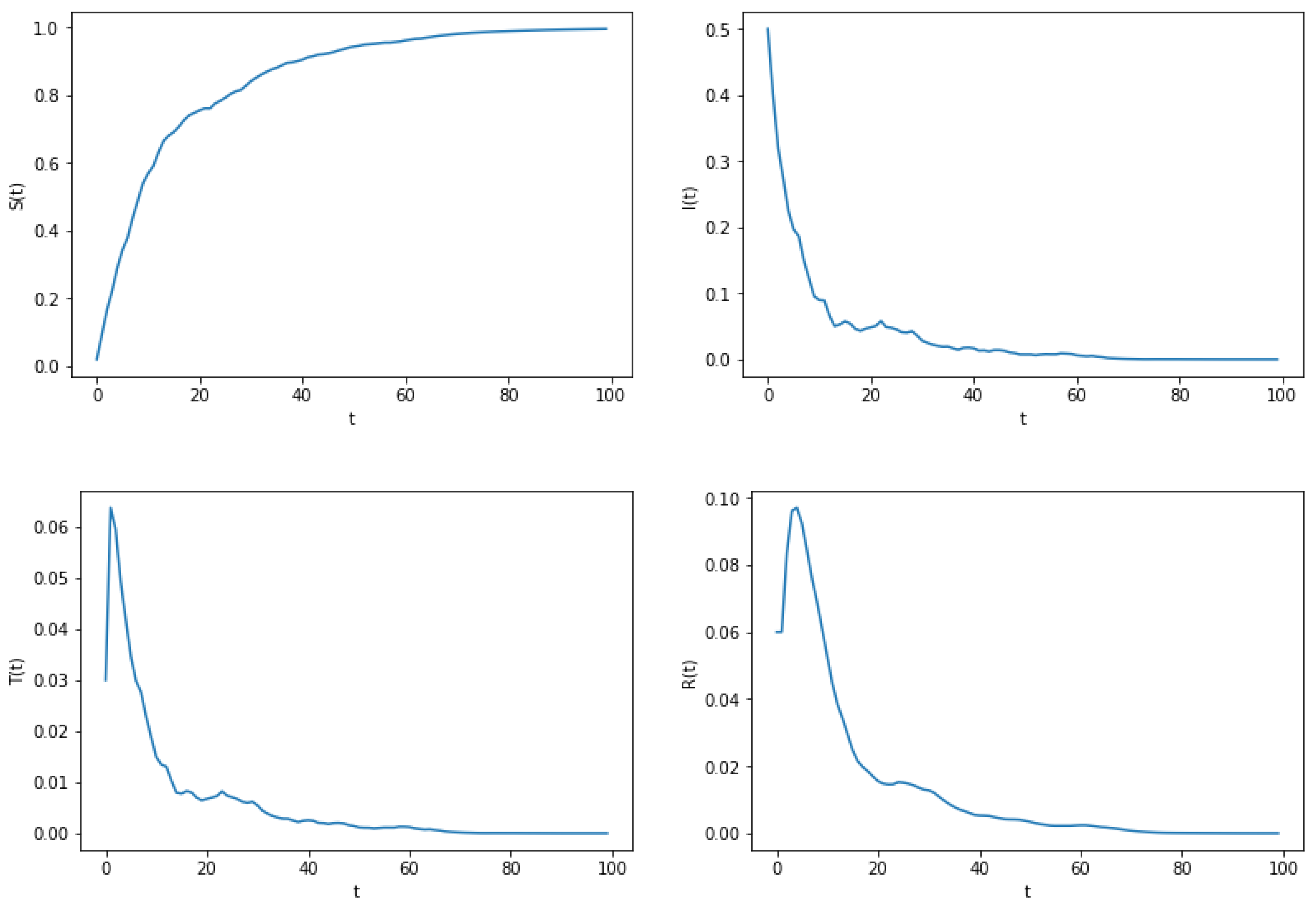
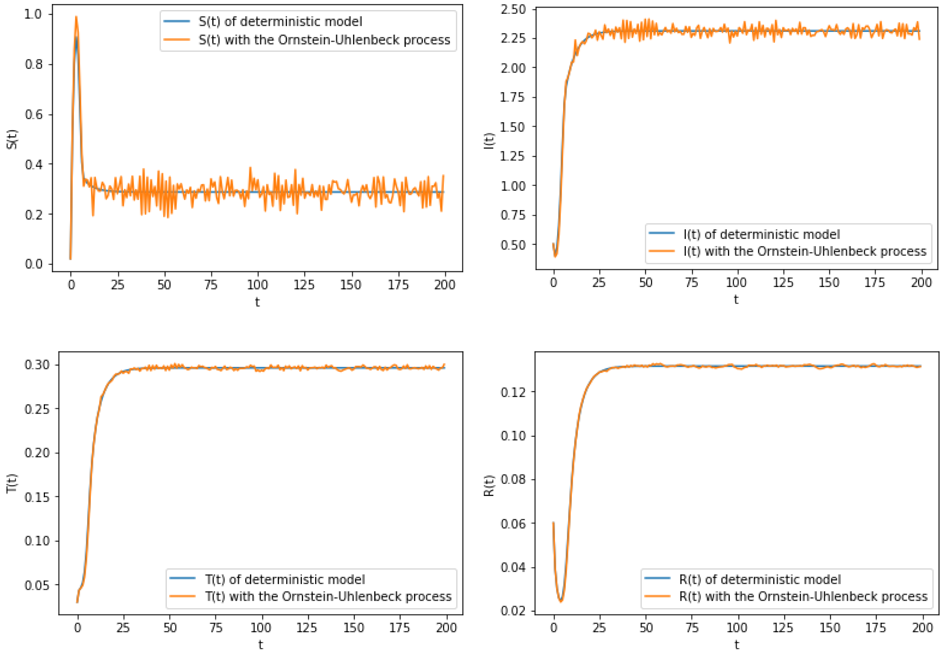
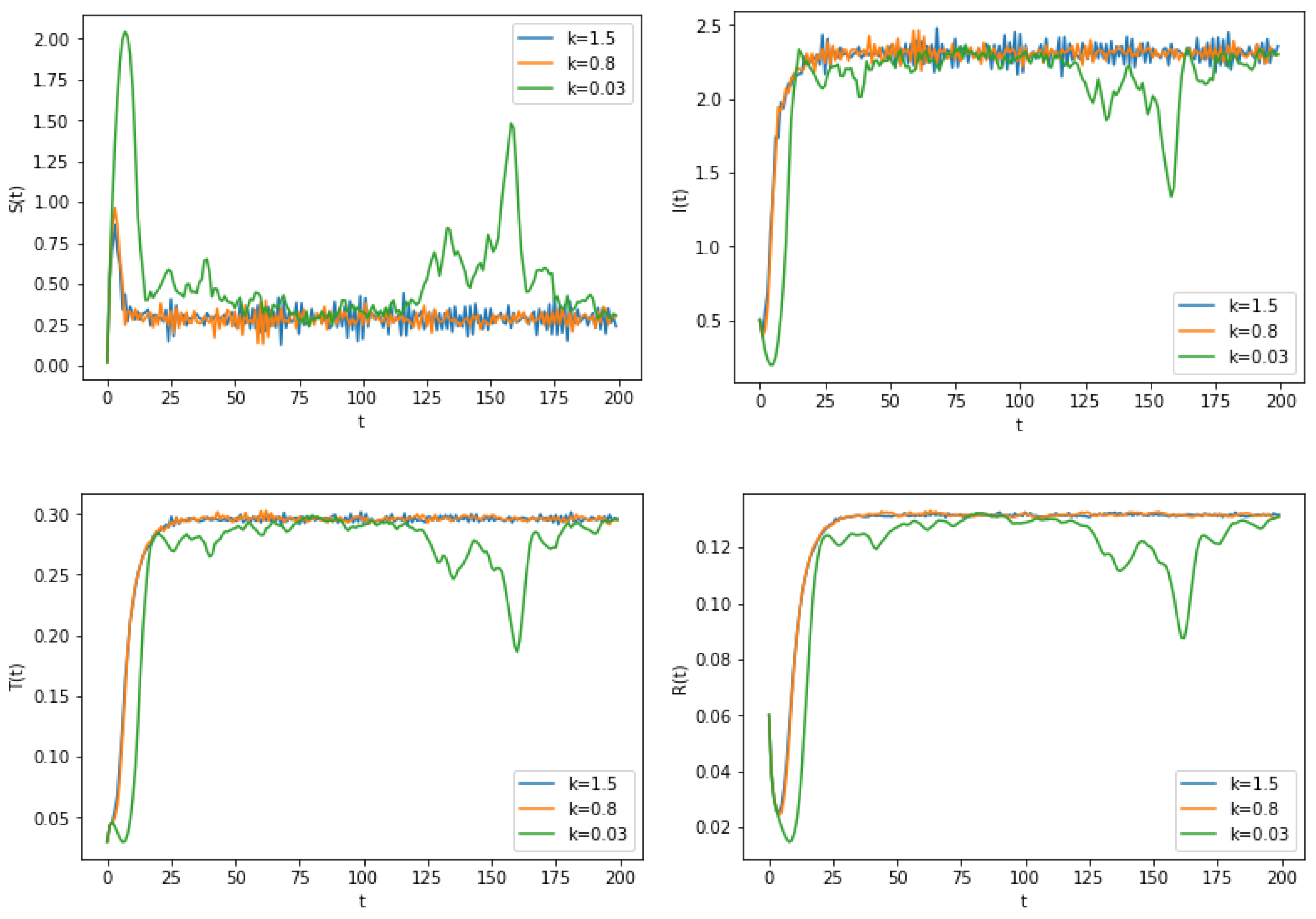
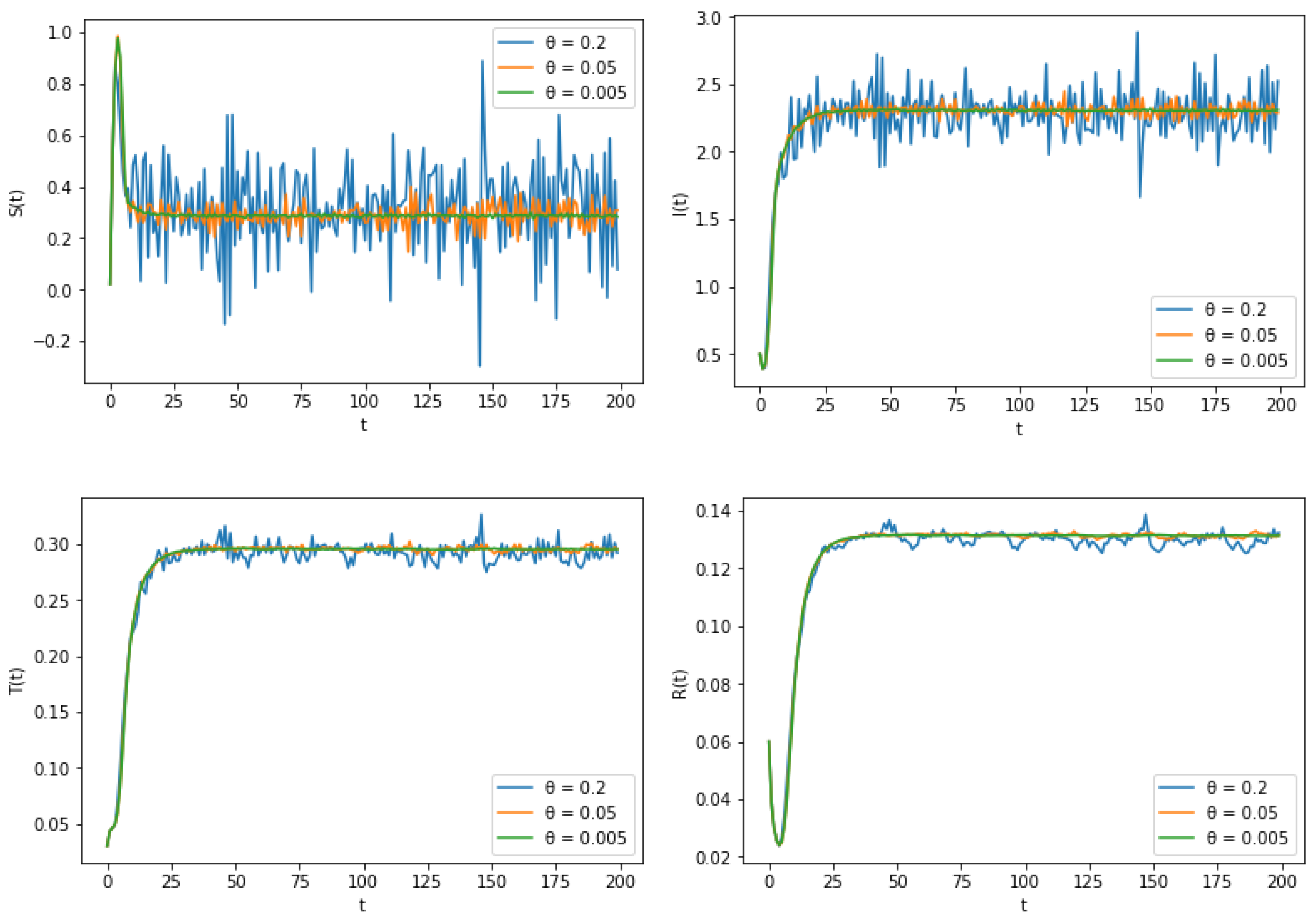
6. Numerical Simulation

In order to verify the correctness of the above proof, numerical simulation results are provided in this section. To begin with, we choose to simulate the model numerically using the Milstein method. Some parameter values in the model are taken from [8,9,10,11,12,13]. We then discretize the model (5) to obtain the following corresponding discretized model:

$$\left\{\begin{array}{cc}\hfill S_{i+1}=& S_i+[A-(\beta +m_i)S_i{I}_i-\xi S_i+p{R}_i]\Delta t,\hfill \\ \hfill I_{i+1}=& I_i+[(\beta +m_i)S_i{I}_i-(\xi +d+\sigma )I_i]\Delta t,\hfill \\ \hfill T_{i+1}=& T_i+[\sigma I_i-(\xi +\gamma +g)T_i]\Delta t,\hfill \\ \hfill R_{i+1}=& R_i+[\gamma T_i-(\xi +p)R_i]\Delta t,\hfill \\ \hfill m_{i+1}=& m_i-k{m}_i\Delta t+\theta h_i\sqrt{\Delta t}+\frac{{\theta }^2}{2}(h_i^2-1)\Delta t.\hfill \end{array}\right.$$

Example 1. 

Assume the parameters $A=0.5, \beta =0.75,$ $\xi =0.15, p=0.3,$ $d=0.015, \sigma =0.05,$ $\gamma =0.2, g=0.04,$ $k=0.8,\theta =0.05$ and the starting points in the below examples are all $\left(S\right(0),I(0),T(0),R(0),$ $m\left(0\right))=(0.02,0.5,0.03,0.06,-0.9)$. Note that $R_0^S\approx 11.1389>1$ satisfies the requirement of Theorem 3. Intuitively, it can be seen that the values of the histogram revolve around $P^{*}=(S^{*},I^{*},T^{*},R^{*})\approx (0.286667,2.309177,0.296048,$ $0.131577)$ of the deterministic model. The solution $\left(S\right(t),I(t),T(t),R(t),m(t\left)\right)$ of system (4) obeys the normal density function $\Phi (S,I,T,R,m)\sim \mathbb{N}({(0.28667,2.30918,0.29605,0.13158,0)}^T,\Sigma )$. The matrix Σ is represented as

$$\Sigma =1\times {10}^{-4}\left(\begin{array}{ccccc}10.197829& -9.762230& -0.177322& -0.082040& -39.042279\\ -9.762230& 9.360669& 0.160540& 0.076008& 37.471400\\ -0.177322& 0.160540& 0.009003& 0.002716& 0.589101\\ -0.082040& 0.076008& 0.002716& 0.001207& 0.317093\\ -39.042279& 37.471400& 0.589101& 0.317093& 156.363696\end{array}\right).$$

From this, the following four marginal density functions are derived:

$${\Phi }_S\left(S\right)=\frac{1}{\sqrt{2\pi }{\phi }_1}{e}^{-\frac{{(S-S^{*})}^2}{2{\phi }_1^2}}=12.492697e^{-490.300445{(S-0.286667)}^2},$$

$${\Phi }_I\left(I\right)=\frac{1}{\sqrt{2\pi }{\phi }_2}{e}^{-\frac{{(I-I^{*})}^2}{2{\phi }_2^2}}=13.039370e^{-534.149840{(I-2.309177)}^2},$$

$${\Phi }_T\left(T\right)=\frac{1}{\sqrt{2\pi }{\phi }_3}{e}^{-\frac{{(T-T^{*})}^2}{2{\phi }_3^2}}=420.457136e^{-555383.953048{(T-0.296048)}^2},$$

$${\Phi }_R\left(R\right)=\frac{1}{\sqrt{2\pi }{\phi }_4}{e}^{-\frac{{(R-R^{*})}^2}{2{\phi }_4^2}}=1148.231844e^{-4141990.007581{(R-0.131577)}^2}.$$

According to Theorem 2, there exists an ergodic stationary distribution for system (4). The frequency histograms of $S\left(t\right),I\left(t\right),T\left(t\right)$ and $R\left(t\right)$ are given in Figure 1. Also in Figure 1, it can be seen that the marginal density function of $\Phi (S,I,T,R)$ given in Theorem 3 is in general agreement with the corresponding frequency histogram.

Example 2. 

Assume the parameters $A=0.05,$ $\beta =0.09,$ $\xi =0.05,$ $p=0.3,$ $d=0.015,$ $\sigma =0.115,$ $\gamma =0.7,$ $g=0.04,$ $k=0.8,$ $\theta =0.14$. At this point, $R_0^E\approx 0.9906<1$ makes Theorem 4 hold. Figure 2 simulates the population sizes of $S\left(t\right)$, $I\left(t\right)$, $T\left(t\right)$ and $R\left(t\right)$, respectively. As can be seen from Figure 2, the population size of $S\left(t\right)$ stabilizes with probability 1 after a period of time; the population sizes of $I\left(t\right)$, $T\left(t\right)$ and $R\left(t\right)$ are 0 after a period of time, which indicates disease extinction.

Example 3. 

Assume that the parameter values in group (a) are the values taken in Example 2, and the parameter values in group (b) are the values taken in Example 1. Through 10,000 random simulations, Figure 3 plots the expectations and standard deviations for the four categories. From Figure 3, it can be seen that in case (a) the disease will disappear, while in case (b) the disease will develop into an epidemic.

Example 4. 

Consider the corresponding discretized deterministic SITRS model

$$\left\{\begin{array}{cc}\hfill S_{i+1}=& S_i+[A-\beta S_i{I}_i-\xi S_i+p{R}_i]\Delta t,\hfill \\ \hfill I_{i+1}=& I_i+[\beta S_i{I}_i-(\xi +d+\sigma )I_i]\Delta t,\hfill \\ \hfill T_{i+1}=& T_i+[\sigma I_i-(\xi +\gamma +g)T_i]\Delta t,\hfill \\ \hfill R_{i+1}=& R_i+[\gamma T_i-(\xi +p)R_i]\Delta t.\hfill \end{array}\right.$$

Assume these parameters use the same values as in Example 1. Substitute the mean-reverting process into model (1) and transform it to the stochastic SITRS model. Figure 4 simulates a comparison plot between the stochastic model combining the mean-reverting process and the deterministic model. It can be seen that the sample trajectories of $S\left(t\right)$, $I\left(t\right)$, $T\left(t\right)$ and $R\left(t\right)$ of the stochastic model combining the mean-reverting process oscillate around the sample trajectories of $S\left(t\right)$, $I\left(t\right)$, $T\left(t\right)$ and $R\left(t\right)$ of the deterministic model.

Example 5. 

To study the impact of regression rate k on disease progression, maintain the other parameter values selected from Example 1 and select different regression rates k. Here, we choose the cases of $k=1.5$, $k=0.8$ and $k=0.03$, respectively. From the sample trajectories of $S\left(t\right),I\left(t\right),T\left(t\right)$ and $R\left(t\right)$ for different values of k in Figure 5, it can be seen that as k decreases, the oscillations of the sample trajectories become larger and the disease becomes more and more unstable.

Example 6. 

With the aim of exploring the role of fluctuation intensity θ in disease progression, maintain the other parameter values selected from Example 1 and select different regression rates θ. Here, we choose the cases of $\theta =0.2$, $\theta =0.05$ and $\theta =0.005$, respectively. From the sample trajectories of $S\left(t\right),I\left(t\right),T\left(t\right)$ and $R\left(t\right)$ for different values of θ in Figure 6, it can be seen that the oscillation of the sample trajectories becomes larger and the disease becomes more and more unstable as θ increases.

7. Conclusions

Cholera outbreaks have been frequent in recent years and the situation is critical. This shows that our knowledge of cholera is still inadequate, that the means of prevention and control are not perfect and that the dynamics of the spread of the epidemic are very complex. In this work, we highlight the stochastic SITRS cholera epidemic model with an Ornstein–Uhlenbeck process. In general, the existing literature always uses white noise to model fluctuations in the environment. However, on this basis, we adopt a new way of introducing random disturbances in the system, namely the Ornstein–Uhlenbeck process. This not only enriches the research on the modeling aspects of cholera epidemics, but also provides us with new insights to control the epidemiology of cholera epidemics. To assure that system (4) is mathematically and biologically justifiable, we prove that the system has a global solution. We then delve into the dynamics of system (4). More specifically, the results of the analyses in this paper are shown below:

(1) Theorem 2 proves that in the presence of disease persistence (i.e., when $R_0^S=R_0-\frac{A\theta }{\sqrt{\pi k}\xi (\xi +d+\sigma )}>1$), system (4) has an ergodic stationary distribution, as shown in Figure 1.

(2) With the help of the solution of the relevant five-dimensional Fokker–Planck equation in Theorem 3, we develop an exact expression for the probability density function of model (4) near the quasi-endemic equilibrium. As shown in Figure 1, we plot a graph of the probability density function.

(3) In Theorem 4, when $R_0^E=R_0+\frac{A\theta }{\sqrt{\pi k}\xi (\xi +d+\sigma )}<1$, the disease tends exponentially to extinction. Figure 2 verifies that under conditions satisfying Theorem 4, the population $I\left(t\right)$ infected with cholera disease converges to 0, and thus cholera disease becomes extinct. As a result, changing the values of the parameters in $R_0^E$ so that they fulfill the conditions of Theorem 4 can help us control the epidemic of cholera disease. This provides us with a theoretical basis for controlling the epidemic of cholera disease.

(4) For numerical simulations, we also plot Figure 5 and Figure 6 by picking different values of $\theta$ and k. Numerically, we also find a meaningful conclusion: smaller regression rates or larger fluctuation intensities make the stochastic system more volatile.

However, there are still many important topics that deserve further research. Firstly, due to the limitations of existing methods, the thresholds for disease extinction and prevalence have not been harmonized. Therefore, the identification of uniform thresholds for disease extinction and prevalence deserves further exploration. Secondly, there is no unique approach to analyzing stochastic systems, and future work could consider more comprehensive and rational ones [37,38]. Finally, in this paper we have only analyzed the kinetic behavior of stochastic SITRS models with treatment compartments. One could build more realistic and important models, for example, studying cholera infectious disease models with more compartments and the effect of a mean-reverting process perturbing other parameters on the dynamics of cholera epidemic transmission.

References

1. Ma, Z.; Zhou, Y.; Wu, J. Modeling and Dynamics of Infectious Diseases, 1st ed.; Higher Education Press: Beijing, China, 2009; pp. 1–35. [Google Scholar]
2. Cai, Y.; Kang, Y.; Banerjee, M.; Wang, W. A stochastic epidemic model incorporating media coverage. Commun. Math. Sci. 2016, 14, 893–910. [Google Scholar] [CrossRef]
3. World Health Organization (WHO). Cholera-Global Situation. Available online: https://www.who.int/emergencies/disease-outbreak-news/item/2023-DON437 (accessed on 11 February 2023).
4. Beryl, M.O.; George, L.O.; Fredrick, N.O. Mathematical analysis of a cholera transmission model incorporating media coverage. Int. J. Pure. Appl. Math. 2016, 111, 219–231. [Google Scholar] [CrossRef]
5. Fatima, S.; Krishnarajah, I.; Jaffar, M.Z.A.M.; Adam, M.B. A mathematical model for the control of cholera in Nigeria. Res. J. Environ. Earth Sci. 2014, 6, 321–325. [Google Scholar] [CrossRef]
6. Nelson, E.J.; Harris, J.B.; Glenn, M.J.; Galderwood, S.B.; Camilli, A. Cholera transmission: The host, pathogen and bacteriophage dynamic. Nat. Rev. Microbiol. 2009, 7, 693–702. [Google Scholar] [CrossRef] [PubMed]
7. Su, T.; Zhang, X. Stationary distribution and extinction of a stochastic generalized SEI epidemic model with Ornstein-Uhlenbeck process. Appl. Math. Lett. 2023, 143, 108690. [Google Scholar] [CrossRef]
8. He, J.; Bai, Z. Global hopf bifurcation of a cholera model with media coverage. Math. Biosci. Eng. 2023, 20, 18468–18490. [Google Scholar] [CrossRef]
9. Lemos-Paiao, A.P.; Silva, C.J.; Torres, D.F.M. A cholera mathematical model with vaccination and the biggest outbreak of world’s history. AIMS Math. 2018, 3, 448–463. [Google Scholar] [CrossRef]
10. Zhou, X.; Shi, X.; Wei, M. Dynamical behavior and optimal control of a stochastic mathematical model for cholera. Chaos Solitons Fractals 2022, 156, 111854. [Google Scholar] [CrossRef]
11. Hartley, D.M.; Morris, J.G., Jr.; Smith, D.L. Hyperinfectivity: A critical element in the ability of V. cholerae to cause epidemics? PLoS Med. 2005, 3, e7. [Google Scholar] [CrossRef]
12. Lemos-Paiao, A.P.; Silva, C.J.; Torres, D.F.M. An epidemic model for cholera with optimal control treatment. J. Comput. Appl. Math. 2017, 318, 168–180. [Google Scholar] [CrossRef]
13. Mwasa, A.; Tchuenche, J.M. Mathematical analysis of a cholera model with public health interventions. Biosystems 2011, 105, 190–200. [Google Scholar] [CrossRef] [PubMed]
14. Wang, X.; Yang, J.; Han, Y. Threshold dynamics of a chronological age and infection age structured cholera model with Neumann boundary condition. Z. Angew. Math. Phys. 2023, 74, 170. [Google Scholar] [CrossRef]
15. Jiang, T.; Wang, J. Modeling and analysis of a diffusive cholera model with seasonally forced intrinsic incubation period and bacterial hyperinfectivity. J. Math. Anal. Appl. 2023, 527, 127414. [Google Scholar] [CrossRef]
16. Tilahun, G.T.; Woldegerima, W.A.; Wondifraw, A. Stochastic and deterministic mathematical model of cholera disease dynamics with direct transmission. Adv. Differ. Equ. 2020, 2020, 670. [Google Scholar] [CrossRef]
17. Zhou, Y.; Jiang, D. Dynamical behavior of a stochastic SIQR epidemic model with Ornstein-Uhlenbeck process and standard incidence rate after dimensionality reduction. Commun. Nonlinear Sci. Numer. Simul. 2023, 116, 106878. [Google Scholar] [CrossRef]
18. Zhang, X.; Zhang, X. Threshold behaviors and density function of a stochastic parasite-host epidemic model with Ornstein–Uhlenbeck process. Appl. Math. Lett. 2024, 153, 109079. [Google Scholar] [CrossRef]
19. Bao, K.; Rong, L.; Zhang, Q. Analysis of a stochastic SIRS model with interval parameters. Discret. Contin. Dyn. Syst. Ser. B 2019, 24, 4827–4849. [Google Scholar] [CrossRef]
20. Liu, Q.; Jiang, D.; Hayat, T.; Alsaedi, A. Dynamical behavior of a stochastic epidemic model for cholera. J. Frankl. Inst. 2019, 356, 7486–7514. [Google Scholar] [CrossRef]
21. Zaho, Y.; Lin, Y.; Jiang, D.; Mao, X.; Li, Y. Stationary distribution of stochastic SIRS epidemic model with standard incidence. Discret. Contin. Dyn. Syst. Ser. B 2016, 21, 2363–2378. [Google Scholar] [CrossRef]
22. Zhang, X.; Yuan, R. A stochastic chemostat model with mean-reverting Ornstein-Uhlenbeck process and Monod-Haldane response function. Appl. Math. Comput. 2021, 394, 125833. [Google Scholar] [CrossRef]
23. Allen, E. Environmental variability and mean-reverting processes. Discret. Contin. Dyn. Syst. Ser. B 2016, 21, 2073–2089. [Google Scholar] [CrossRef]
24. Kutoyants, Y.A. Statistical Inference for Ergodic Diffusion Processes, 1st ed.; Springer: London, UK, 2004; pp. 50–103. [Google Scholar]
25. Alshammari, F.S.; Akyildiz, F.T. Epidemic waves in a stochastic SIRVI epidemic model incorporating the Ornstein-Uhlenbeck process. Mathematics 2023, 11, 3876. [Google Scholar] [CrossRef]
26. Zhou, B.; Jiang, D.; Hayat, T. Analysis of a stochastic population model with mean-reverting Ornstein-Uhlenbeck process and Allee effects. Commun. Nonlinear Sci. Numer. Simul. 2022, 111, 106450. [Google Scholar] [CrossRef]
27. Wu, S.; Yuan, S.; Lan, G.; Zhang, T. Understanding the dynamics of hepatitis B transmission: A stochastic model with vaccination and Ornstein-Uhlenbeck process. Appl. Math. Comput. 2024, 476, 128766. [Google Scholar] [CrossRef]
28. Zhou, B.; Jiang, D.; Han, B.; Hayat, T. Threshold dynamics and density function of a stochastic epidemic model with media coverage and mean-reverting Ornstein–Uhlenbeck process. Math. Comput. Simul. 2022, 196, 15–44. [Google Scholar] [CrossRef]
29. Liu, Q. A stochastic predator-prey model with two competitive preys and Ornstein-Uhlenbeck process. J. Biol. Dyn. 2023, 17, 2193211. [Google Scholar] [CrossRef] [PubMed]
30. Zhang, Z.; Liang, G.; Chang, K. Stationary distribution of a reaction-diffusion hepatitis B virus infection model driven by the Ornstein-Uhlenbeck process. PLoS ONE 2023, 18, e0292073. [Google Scholar] [CrossRef] [PubMed]
31. Mao, X. Stochastic Differential Equations and Applications, 2nd ed.; Horwood: Chichester, UK, 2008; pp. 149–155. [Google Scholar]
32. Du, N.H.; Nguyen, D.H.; Yin, G.G. Conditions for permanence and ergodicity of certain stochastic predator–prey models. J. Appl. Probab. 2016, 53, 187–202. [Google Scholar] [CrossRef]
33. Meyn, S.P.; Tweedie, R.L. Stability of Markovian processes III: Foster-Lyapunov criteria for continuous-time processes. Adv. Appl. Probab. 1993, 25, 518–548. [Google Scholar] [CrossRef]
34. Dieu, N.T. Asymptotic Properties of a Stochastic SIR Epidemic Model with Beddington-DeAngelis Incidence Rate. J. Dyn. Differ. Equ. 2018, 30, 93–106. [Google Scholar] [CrossRef]
35. Roozen, H. An asymptotic solution to a two-dimensional exit problem arising in population dynamics. SIAM J. Appl. Math. 1989, 49, 1793–1810. [Google Scholar] [CrossRef]
36. Zhang, X.; Su, T.; Jiang, D. Dynamics of a Stochastic SVEIR Epidemic Model Incorporating General Incidence Rate and Ornstein–Uhlenbeck Process. J. Nonlinear Sci. 2023, 33, 76. [Google Scholar] [CrossRef]
37. Yang, X.; Zhang, J. Systems of reflected stochastic PDEs in a convex domain: Analytical approach. J. Differ. Equ. 2021, 284, 350–373. [Google Scholar] [CrossRef]
38. Baccouch, M.; Temimi, H.; Ben-Romdhane, M. A discontinuous Galerkin method for systems of stochastic differential equations with applications to population biology, finance, and physics. J. Comput. Appl. Math. 2021, 388, 113297. [Google Scholar] [CrossRef]
Figure 1. The histogram and marginal density function of model (4). Parameter values: ( A , β , ξ , p , d , σ , γ , g , k , θ ) = ( 0.5 , 0.75 , 0.15 , 0.3 , 0.015 , 0.05 , 0.2 , 0.04 , 0.8 , 0.05 ) .
Mathematics 12 02163 g001
Figure 2. The trajectories of S ( t ) , I ( t ) , T ( t ) and R ( t ) in model (4) during disease extinction. Parameter values: ( A , β , ξ , p , d , σ , γ , g , k , θ ) = ( 0.05 , 0.09 , 0.05 , 0.3 , 0.015 , 0.115 , 0.7 , 0.04 , 0.8 , 0.14 ) .
Mathematics 12 02163 g002
Figure 3. Computer simulations for expectation and standard deviation of the model (4). Parameter values: ( a ) ( A , β , ξ , p , d , σ , γ , g , k , θ ) = ( 0.05 , 0.09 , 0.05 , 0.3 , 0.015 , 0.115 , 0.7 , 0.04 , 0.8 , 0.14 ) ; ( b ) : ( A , β , ξ , p , d , σ , γ , g , k , θ ) = ( 0.5 , 0.75 , 0.15 , 0.3 , 0.015 , 0.05 , 0.2 , 0.04 , 0.8 , 0.05 ) .
Mathematics 12 02163 g003
Figure 4. The trajectories of S ( t ) , I ( t ) , T ( t ) and R ( t ) of stochastic model (4) with the mean-reverting process and deterministic model (1). Parameter values: ( A , β , ξ , p , d , σ , γ , g , k , θ ) = ( 0.5 , 0.75 , 0.15 , 0.3 , 0.015 , 0.05 , 0.2 , 0.04 , 0.8 , 0.05 ) .
Mathematics 12 02163 g004
Figure 5. The trajectories of S ( t ) , I ( t ) , T ( t ) and R ( t ) for model (4) with different regression rates k. Parameter values: ( A , β , ξ , p , d , σ , γ , g , θ ) = ( 0.5 , 0.75 , 0.15 , 0.3 , 0.015 , 0.05 , 0.2 , 0.04 , 0.05 ) .
Mathematics 12 02163 g005
Figure 6. The trajectories of S ( t ) , I ( t ) , T ( t ) and R ( t ) for model (4) with different regression rates θ . Parameter values: ( A , β , ξ , p , d , σ , γ , g , k ) = ( 0.5 , 0.75 , 0.15 , 0.3 , 0.015 , 0.05 , 0.2 , 0.04 , 0.8 ) .
Mathematics 12 02163 g006
Disclaimer/Publisher’s Note: The statements, opinions and data contained in all publications are solely those of the individual author(s) and contributor(s) and not of MDPI and/or the editor(s). MDPI and/or the editor(s) disclaim responsibility for any injury to people or property resulting from any ideas, methods, instructions or products referred to in the content.