Abstract
The ordinary 3D wave equation for nondissipative, homogeneous, isotropic media admits solutions where the point sources are permitted to move, but as shown in this paper, it does not admit solutions where the receiver is allowed to move. To overcome this limitation, a new wave equation that permits both the receiver and the source to move is derived in this paper. This new wave equation is a generalization of the standard wave equation, and it reduces to the standard wave equation when the receiver is at rest. To derive this new wave equation, we first mathematically define a diverging spherical wave caused by a stationary point source. From this purely mathematical definition, the wave equation for a stationary source and a moving receiver is derived, together with a corresponding free-space Green function. Utilizing the derived Green function, it is shown that unlike the standard wave equation this new wave equation also permits solutions where both the receiver and the source are permitted to move. In conclusion, this paper demonstrates that, instead of an ordinary wave equation, the wave equation for a moving source and a moving receiver governs the waves emitted by moving point sources and received by moving receivers. This new wave equation has possible applications in acoustics, electrodynamics, and other physical sciences.
MSC:
35L05
1. Introduction
One of the most important partial differential equations in physics is the ordinary three-dimensional wave equation [1,2]. It was first derived by Leonhard Euler in the 18th century to describe the propagation of three-dimensional acoustic waves [3,4]. Although originally conceived to describe the propagation of acoustic waves without losses in homogeneous isotropic media, it was later found that under the same conditions (these conditions assume the homogeneity and isotropy of media and the wave propagation without losses.), the ordinary wave equation describes a variety of wave phenomena such as the propagation of waves in solids [5], the propagation of mechanical stress waves [6], and the propagation of seismic waves [7], and as shown by Maxwell in the 19th century [8], the ordinary wave equation describes the propagation of electromagnetic waves.
Regardless of whether the wave equation describes a mechanical, acoustic, or electromagnetic wave, the ordinary three-dimensional wave equation reads as follows:
where u is the displacement, c is the velocity of the wave propagation, t is the time, and is the three-dimensional Laplace operator. In general, the wave Equation (1) describes the propagation of a displacement, or a disturbance, propagating from the source to the receiver with finite velocity c [9]. In the case of an acoustic wave, the function u represents the pressure or the velocity potential [10,11,12]. For an electromagnetic wave, the function u can be any Cartesian component of an electric or magnetic field [13,14].
A particularly important class of solutions to the ordinary wave equation are those that involve moving point sources. In the field of electrodynamics, the Liénard–Wiechert scalar and vector potentials are examples of such solutions [15,16]. These time-retarded potentials are widely used for advanced electromagnetic calculations such as synchrotron, undulator, and radar radiation [17,18,19]. For example, the scalar Liénard–Wiechert potential takes the following mathematical form:
where is the distance between the moving source and the stationary receiver (in this paper we use the term receiver instead of the more common term observer.), q is the amount of charge given in Coulombs, is the position vector of a stationary receiver, is the position vector of the moving source, and is the retarded time that satisfies the following causal relationship:
Furthermore, the vectors and are given by
Solutions to the ordinary wave equation for moving sources are also found in the field of acoustics. For example, Schmidt and Kuperman derived a solution to the ordinary wave equation for a harmonic point source moving with constant velocity along a straight line [20]. Obrezanova and Rabinovich derived a two-dimensional solution for a harmonic point source moving along an arbitrary path [21]. Lim and Ozard derived a solution for a harmonic acoustic source moving along an arbitrary trajectory in 3D [22] that has a mathematical form similar to the Liénard–Wiechert scalar potential.
Modifying any of these moving point source solutions to accommodate a moving receiver results in a violation of the ordinary wave equation. For example, if the receiver starts to move, then its position becomes a function of time, i.e., . As will be demonstrated later in this paper, if one substitutes by in Equation (2), then u is no longer the solution to the ordinary wave equation. The same applies to the acoustic point source solutions mentioned in references [20,21,22].
Thus, the ordinary wave equation has the ability to describe waves caused by moving sources, but it cannot describe the waves seen by the moving receiver. It is shown in this paper that a wave equation that admits solutions where both the receiver and the source are permitted to move takes the following mathematical form:
where is the velocity vector of the moving receiver, and the operator represents the operator applied twice. If the receiver is stationary, then , and the Equation (6) reduces to an ordinary wave equation.
The proof that for moving receivers the wave Equation (6) is valid instead of the ordinary wave equation is organized as follows: in Section 2, we first mathematically define a wave function caused by a stationary point source and received by a moving receiver. In Section 3, we use this wave function to derive a wave Equation (6) for the specific case of a moving receiver and a stationary source. Then, in Section 4, Green’s function for Equation (6) is derived. Finally, in Section 5, by using the derived Green’s function, solutions to the wave Equation (6) are found where both the receiver and the source are permitted to move. This means that Equation (6) is the correct wave equation when both the source and the receiver are moving.
In conclusion, it is shown that instead of an ordinary wave equation, Equation (6) is the governing wave equation when both the receiver and the source are permitted to move. If the receiver becomes stationary, then the wave Equation (6) reduces to an ordinary wave equation. This means that the ordinary wave equation can be considered a particular case of the wave equation for a moving receiver and a moving source. These findings are summarized in Table 1, where the wave equation for a moving source and a moving receiver and its point-source solution are compared to the ordinary wave equation and respective point-source solution.

Table 1.
Comparison of the ordinary wave equation and the wave equation for a moving source and a moving receiver. The ordinary wave equation does not allow motion of the receiver, while the wave equation for a moving source and a moving receiver allows motion of both the source and the receiver.
Therefore, the novelty presented in this work is that a new wave equation is discovered that, unlike the ordinary wave equation, allows both the source and the receiver to be in motion. This new wave equation can be considered an extension of the three-dimensional ordinary wave equation discovered by Euler in the 18th century, which has remained unchanged until the present day. This new wave equation does not mean that Euler’s wave equation is generally incorrect; it is correct under certain conditions; that is, it is revealed in this paper that it is correct if the receiver is not in motion. If, on the other hand, the receiver is in motion, then the wave equation for a moving source and a moving receiver is the governing differential equation and not Euler’s.
2. Free Space Wave Function for a Stationary Source and Moving Receiver
In this section, we mathematically describe a wave caused by a stationary point source and received by a moving receiver. The wave is simply a disturbance emitted by the source at retarded time that travels towards the receiver with finite velocity c. Because the disturbance travels with finite velocity, this disturbance arrives at the moving receiver at the time . This causal relationship can be represented by the following equation:
where we declare that time t is an independent variable.
In the expression (7), the function represents the distance between the location of the source and the location of the moving receiver at the time t when the wave emitted from the source at time intercepts the receiver. This distance can be written as
where the vector is the position vector of the moving receiver at the time t of wave reception, and the vector is the position vector of a stationary source.
A simple way to define a wave function u that represents a disturbance traveling in time with velocity c is by declaring
where F is any function twice differentiable. By substituting Equation (7) into Equation (9), we can equivalently write
Equations (9) and (10) represent a disturbance that has the value at the time of emission . This disturbance travels towards the receiver with velocity c, and it intercepts the moving receiver at time t. As indicated in Figure 1, at the time of interception, the disturbance still has the value .
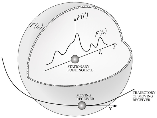
Figure 1.
A stationary point source emits a disturbance that has the value at time . This disturbance travels with velocity c and spreads equally in all directions. At moment , the disturbance carrying the value intercepts the receiver moving with velocity .
From Equations (9) and (10), it is also clear that the wave function u represents a spherical wave spreading equally in all directions away from the source. If something emits spherical waves from position , this also means that there is a point source located at position .
Furthermore, Equations (9) and (10) imply that the amplitude of function u does not change as the wave travels away from the source. In nature, point sources usually generate diverging spherical waves whose amplitude is inversely proportional to the distance from the source. For example, an acoustic point source generates diverging spherical waves [23,24], and the point source of electric potential waves and magnetic vector potential waves generates diverging spherical waves [25,26]. Therefore, if the function u is to represent the wave generated by a physical point source, the wave function u must take the following mathematical form:
If a constant is added to the argument of the function F, the function u still satisfies the wave equation. Thus, for the sake of completeness, and for reasons that will become apparent in Section 4 of this paper, we rewrite the wave function u as follows:
where a is any real constant. As shown in Section 4, this particular mathematical form of the wave function allows us to derive Green’s function for the wave equation for a moving receiver in a relatively straightforward manner.
3. The Wave Equation for a Moving Receiver and a Stationary Source
In this section, we derive a wave equation for a stationary point source and a moving receiver. Here, the position of the receiver is considered a function of time t, i.e., , and the position vector of the stationary source is not considered a function of time:
The distance between the source at the time of wave emission and the receiver at the time of wave interception is a function of time:
Although the source is stationary, it still emits waves (disturbances) at retarded time that travel to the receiver with velocity c. These disturbances arrive at moving the receiver at time t, and the causal relationship connecting the retarded time and the present time is expressed by the following equation:
For this reason, the wave function u describing the disturbance traveling in time towards the moving receiver, and emitted by the stationary source, is still described by the function of retarded time :
The derivatives of the retarded time with respect to variables are non-zero and these can be obtained by differentiating Equation (16) with respect to variable .
The derivative of the wave function u given by Equation (17) with respect to variable can be calculated using the chain rule:
where R is a shorthand notation for , and where and . Note that because of Equation (7), the derivative of the retarded time with respect to variable is non-zero. This follows from Equation (7), where we declared the variable t as an independent variable; therefore, the retarded time is a function of the variable t, the constant vector , and the vector function .
By differentiating Equation (18) with respect to the variable , the second order derivative of the wave function u is obtained as
where . The Laplacian of the function u can now be written as the sum:
By differentiating Equation (16) with respect to the variable , the following is obtained:
The derivative can be obtained by differentiating Equation (15) with respect to variable as follows:
where is the ith Cartesian component of the unit vector given as
Clearly, because the vector is an unit vector, it can be written
Using Equations (21), (22), and (24), one can calculate the sums found in Equation (20) as
where the symbol represents the 3D Dirac delta function. The expression given by Equation (29) is well-known [27,28] and frequently used in numerous electrodynamics calculations. Its utility can be seen in the computation of electromagnetic fields of point dipoles [29] and the determination of the vector potentials of uniformly moving charges [30].
The divergence of the unit vector can be calculated as
where are Cartesian components of the vector , i.e., . Substituting Equations (25)–(30) into Equation (20) yields:
After cancellation of the appropriate terms on the right-hand side of Equation (31), Equation (31) simplifies to
We now introduce the operator , where is the velocity of the receiver:
By applying the operator to the function u, the following is obtained:
where are Cartesian components of the velocity vector . Substituting Equations (21) and (22) into Equation (34) gives
By differentiating Equation (15), the time derivative is obtained:
Substituting Equation (36) into Equation (35) yields
The second and the fourth right-hand side terms of the equation above cancel, thus we may write
By differentiating Equation (16) with respect to time, one obtains
Substituting Equation (39) into Equation (38) yields
Next, we apply operator to Equation (40) to obtain
where the operator simply means the operator applied twice. Substituting Equations (21) and (22) into Equation (41) gives
Furthermore, substituting Equation (36) into Equation (42) yields
The second and fourth right-hand side terms cancel, therefore
By substituting Equation (39) into Equation (44), it is shown that
Subtracting Equation (45) divided by from Equation (32) yields the wave equation for a stationary source and a moving receiver:
where F is any function such that . This means that the function F can even be a constant, which has applications in electrodynamics [25]. It is also interesting to note that if the receiver becomes stationary, then and the velocity of the receiver . In that case, the wave equation for the stationary source and the moving receiver becomes wave Equation (1).
4. Green’s Function for a Wave Equation for a Moving Receiver and a Stationary Source
The free space Green function for the three-dimensional version of the wave equation is typically derived using the application of a Fourier or Laplace transform [31,32], which is somewhat mathematically involving. For the wave equation given by Equation (1), Green’s function G satisfies the following inhomogeneous wave equation:
Using Fourier’s or Laplace transform, one can solve Equation (47) for the function G to obtain Green’s function for the wave equation in an unbounded domain [33,34]:
which represents the effect of an impulse propagating away from the source located at the position .
We are now interested in finding Green’s function for the wave equation for a moving receiver and a stationary source expressed by Equation (46). Therefore, we need to find the function G that satisfies the following inhomogeneous wave equation:
Instead of using Fourier or Laplace transform to find the function G, we here take a simpler approach that takes advantage of the right-hand side of Equation (46). If in Equation (8) we replace the constant vector by the constant vector , the function u becomes
Because is a constant vector, the function u still satisfies the wave equation for the moving observer and the stationary source given by Equation (46). Now, by letting , where is an independent real variable, the function u becomes
Note that because is an independent variable, the function u still satisfies Equation (46). The function F can be any differentiable function, thus we choose F to be Dirac’s delta function divided by :
With this choice, the function u becomes
Substituting the function u into the Equation (46) yields
The first factor on the right-hand side of Equation (54), i.e., the term , is non-zero only when . In that case, the Dirac delta function becomes
Substituting Equation (55) into Equation (54) yields:
Thus, it is evident that the function u as defined by Equation (53) is indeed Green’s function for the wave equation for a moving receiver and a stationary source:
Note the difference between the Green functions given by Equations (48) and (57): with Equation (57), the receiver is allowed to move, because its position is described by the position vector . With Equation (48), the receiver is not allowed to move, because its position is described by the constant position vector .
5. The Wave Equation for a Moving Source and a Moving Receiver
Thus far, it has been assumed that the wave equation for a moving source and a stationary receiver given by Equation (46) admits only the solutions in which the receiver is allowed to move but the source is stationary. In this section, however, we attempt to find a solution to the wave Equation (46) in which both the source and the receiver are allowed to move. If such a solution exists, it must satisfy the following inhomogeneous wave equation:
Furthermore, if the function u is the solution to the Equation (58), then the distance R between the location of the source at time when the wave was emitted and the location of the moving receiver at time t when this wave arrives at the receiver must be a function of both the retarded time and time t:
Substituting Equation (59) into the causal relationship given by Equation (7) yields:
Note the difference between Equation (46) and Equation (58). In Equation (46), motion of the source is not allowed, while the receiver can move along an arbitrary trajectory. In contrast, Equation (58) allows both the source and the receiver to move along an arbitrary trajectory.
Before we start the mathematical procedure of finding the solution to Equation (58) where both the source and the receiver can move, note that the right-hand side term of Equation (58) is non-zero only when . This can only happen if the source and the receiver occupy the same point in 3D space, that is, if the source and the receiver collide. In that case, the retarded time is equal to the present time t, and we can write
where the solution u can be obtained using the method of Green’s function:
and where denotes the set of real numbers.
Note that by substituting into Equation (57), Green’s function for a moving receiver and a stationary source can also be written as
Because the differential operators ∇ and do not act on the vector , Equation (63) is still the solution to the wave equation for a moving receiver and a stationary source, i.e., to the differential equation . However, this form of Green’s function is required to derive the final result of this section. Substituting Equation (63) into Equation (62) yields
The sifting property of Dirac’s delta function picks out point , thus Equation (64) becomes
Using the following identity involving Dirac’s delta function [35,36]
where is a differentiable function, and is the solution to the equation , one can write Dirac’s delta function under the integral on the right-hand side of Equation (65) as
where is the solution to the following equation:
By comparing Equations (60) and (68), it follows that time is
Differentiating the expression in the denominator of Equation (67), while keeping in mind that t is an independent variable yields
Substituting Equation (70) into Equation (67) yields
Using Equation (69), i.e., , yields
If we assume that , Equation (73) can be written as
Equation (73) can be written in more concise form as
where the vectors and are given as
Furthermore, substituting Equation (74) into Equation (65) yields
Using the sifting property of the Dirac delta function, we can rid ourselves of the integral in Equation (77) to obtain
where , where the retarded time satisfies Equation (60), and where the vector is a function of both time t and retarded time .
Put in other words, the function u is the wave function when both the source and the receiver can move along arbitrary trajectories, and the function u satisfies the wave Equation (61). This means that Equation (46) derived in Section 3 of this paper is not only the wave equation for a moving receiver and a stationary source, but it is also the wave equation for a moving receiver and a moving source.
Note that Equation (78) does not satisfy the ordinary wave equation given by Equation (1). However, if the receiver becomes stationary, then , and consequently, the velocity of the receiver . In such a scenario, the wave equation for a moving source and a moving receiver (61) simplifies to the ordinary wave equation, and the solution (78) also simplifies to the solution to the ordinary wave equation. Thus, it is evident that the ordinary wave equation is a special case of wave Equation (58).
From the point of view of electrodynamics, it is worth noting that if the function F is a constant, such that , and if the velocity of the receiver , then Equation (78) becomes a scalar Liénard–Wiechert potential caused by the moving point charge. This potential is also the solution to the ordinary wave equation, because the receiver is stationary.
6. Summary and Discussion
In Table 1, the results of the investigations conducted in this paper are concisely summarized. The table is divided into two parts: the first deals with the ordinary wave equation, and the second deals with the wave equation for a moving source and a moving receiver. The moving point-source solution to the ordinary wave equation and the corresponding parameters are obtained by setting (and consequently ) in Equation (61). As indicated in Table 1, the ordinary wave equation cannot have solutions where the receiver is in motion.
Although the point source solutions to the ordinary wave equation are obtained from Equation (61) by setting and , these solutions can be verified in a different manner by using the differentiation techniques described in Appendix A. However, verifying the equations given in Table 1 using these differentiation techniques requires a significant amount of mathematical manipulation, which would significantly and unnecessarily lengthen this paper. Alternatively, advanced symbolic computation software such as Mathematica, together with the techniques given in Appendix A, can be employed to verify the equations in Table 1 in a different manner than the one presented in this paper.
The second part of Table 1 presents the wave equation for a moving source and a moving receiver and its general solution for point sources. The equations given in the second part of this table represent a summary of Section 5 of this paper. As indicated in the second part of Table 1, the wave Equation (61) is more general than an ordinary wave equation because it admits solutions for a moving receiver. In fact, it can be concluded that the ordinary wave equation is a particular case of the wave equation for a moving source and a moving receiver when .
Regarding the validation of the wave equation for a moving source and a moving receiver, Table 1 reveals that one may consider that it has already been validated. The wave functions presented in the second part of Table 1 are numerically identical to the wave functions shown in the first part of Table 1. Therefore, if any physical problem produces the wave function described in the first part of Table 1 then it can automatically be extended to moving receivers by using the second part of Table 1. Simply put, if for example a physical problem produces the wave function
where both the receiver and the source are stationary, we know that Equation (79) satisfies the standard inhomogeneous Euler’s wave equation:
Let us now extend the function u to moving receivers by allowing the receiver to move along a certain trajectory, i.e., . The function u now becomes
The function u given by the equation (81) is no longer the solution to the standard wave equation given by equation (80), but it is the solution to the following inhomogeneous equation:
The equation above is the wave equation for a moving source and a moving receiver.
Numerically, there is no difference between the function u given by Equations (79) and (81) because they give the same value for a pair of points and . However, the mathematical description has changed, and therefore the wave equation that the function u satisfies has changed as it now satisfies the wave equation for a moving source and a moving receiver. But if the function u given by Equation (79) together with the governing Equation (80) is physically validated, then Equations (81) and (82) are physically validated as well, because the value of function u remains the same for the pair of points and .
7. Conclusions
The ordinary 3D wave equation for nondissipative, homogeneous, isotropic media has not changed since 1766 when Euler published the 3D wave equation describing the propagation of acoustic waves. Originally, Euler did not specifically consider moving receivers nor moving sources. Only later was it shown that the ordinary 3D wave equation can cope with moving sources. However, this paper reveals that the standard 3D wave equation cannot cope with moving receivers.
Therefore, the aim of this work was to derive a wave equation that allows motion of both the receiver and the source. The derivation of this wave equation was carried out in Section 5, and it was demonstrated that the derived wave equation allows motion of both the receiver and the source. Furthermore, it was shown that the ordinary 3D wave equation is a particular case of the wave equation for a moving source and a moving receiver. Thus, the wave equation for a moving source and a moving receiver can be viewed as the continuation and generalization of Euler’s work on the 3D wave equation.
In addition to this, general point source solutions are derived for both the ordinary wave equation and for the wave equation for a moving source and a moving receiver. These solutions can be adapted for various particular physical problems involving wave propagation without losses in homogeneous isotropic media. Additionally, the free space Green’s function for the wave equation for a moving source and a moving receiver has also been derived.
Lastly, the wave equation for a moving source and a moving receiver has potential applications in physics. In particular, the limitations of Liénard–Wiechert potentials in electrodynamics, namely their inability to represent moving receivers, could be resolved by altering these potentials. This modification could potentially aid with some modern challenges in the field of electrodynamics and possibly with plasmas.
Funding
This research received no external funding, and the APC was funded by the Faculty of Maritime Studies, University of Split, Split, Croatia.
Data Availability Statement
No new data were created or analyzed in this study. Data sharing is not applicable to this article.
Acknowledgments
The author is thankful to Šimun Anđelinović, the former rector of the University of Split, Croatia for moral and other support and for his insightful remarks regarding the origin of Newton’s physics.
Conflicts of Interest
The author declare no conflicts of interest.
Appendix A. Differentiation of Causal Expressions
In this appendix, we derive some mathematical identities that can be used to verify the equations given in Table 1 in a different manner than the one presented in this paper. By differentiating Equation (60) with respect to variable x, where , one obtains
The equation above can be written in a simpler notation:
where is given by Equation (76), the vector is given by Equation (75), and is a Cartesian x component of the vector . From the equation above, it follows that
where the function g is
We can now generalize the result provided by Equation (A3) as
where is the Cartesian component of the vector and . Using the expression (A5), one can now calculate the gradient as
Furthermore, by differentiating Equation (60) with respect to time t, one obtains
The equation above can be written in simpler notation using the vectors and as
where the velocity is the velocity of the receiver. From the equation above, it follows that the derivative is
where the vector is
and where the function f is
One can now use Equations (A6) and (A9) to calculate the gradient, divergence, Laplacian, and the second-order time derivative of the function u given by Equation (78) to verify the equations given in the second part of Table 1. To verify the equations in the first part of Table 1, we set , , . Note that verifying the equations in Table 1 using expressions (A6) and (A9) requires a significant amount of mathematical manipulation; however, advanced symbolic computation software such as Mathematica can significantly aid that task.
References
- Kirkwood, J. Mathematical Physics with Partial Differential Equations; Academic Press: Cambridge, MA, USA, 2013. [Google Scholar]
- Evans, L. Partial Differential Equations; American Mathematical Society: Providence, RI, USA, 1998; Volume 19. [Google Scholar]
- Euler, L. De la Propagation du Son. Mém. Acad. Sci. Berlin 1766, 15, 185–209. [Google Scholar]
- Kline, M. Mathematical Thought from Ancient to Modern Times; Oxford University Press: Oxford, UK, 1972. [Google Scholar]
- Royer, D.; Dieulesaint, E. Elastic Waves in Solids I; Springer: Berlin/Heidelberg, Germany, 2000. [Google Scholar]
- Wang, L. Foundations of Stress Waves; Elsevier: Amsterdam, The Netherlands, 2007. [Google Scholar]
- Krebes, E. Seismic Wave Theory; Cambridge University Press: Cambridge, UK, 2019. [Google Scholar]
- Maxwell, J.C. A dynamical theory of the electromagnetic field. Phil. Trans. R. Soc. 1865, 155, 459–512. [Google Scholar]
- Li, Y.; Wang, C. On a partially synchronizable system for a coupled system of wave equations in one dimension. Commun. Anal. Mech. 2023, 15, 470–493. [Google Scholar] [CrossRef]
- Beranek, L. Acoustics; American Institute of Physics, Inc.: Woodbury, NY, USA, 1986. [Google Scholar]
- Ginsberg, J. Acoustics-A Textbook for Engineers and Physicists; Springer International Publishing AG: Cham, Switzerland, 2018. [Google Scholar]
- Pierce, A. Acoustics—An Introduction to Its Physical Principles and Applications, 3rd ed.; Springer Nature Switzerland AG: Cham, Switzerland, 2019. [Google Scholar]
- Holt, C. Introduction to Electromagnetic Fields and Waves; John Wiley & Sons, Inc.: Hoboken, NJ, USA, 1963. [Google Scholar]
- Felsen, L.; Marcuvitz, N. Radiation and Scattering of Waves; John Wiley & Sons, Inc.: Hoboken, NJ, USA, 1994. [Google Scholar]
- Wiechert, E. Elektrodynamische elementargesetze. Ann. Phys. 1901, 309, 667–689. [Google Scholar] [CrossRef]
- Liénard, A. Champ électrique et magnétique produit par une charge électrique concentrée en un point et animée d’un mouvement quelconque. L’Éclairage Électrique 1898, 16, 5–14. [Google Scholar]
- Arakelyan, S.; Grigoryan, G.; Grigoryan, R. Lienard-Wiechert potentials and synchrotron radiation from a relativistic spinning particle in pseudoclassical theory. Phys. At. Nucl. 2000, 63, 2115–2122. [Google Scholar] [CrossRef]
- Steinbach, A. Electromagnetic theory of range-doppler imaging in laser radar. i: Scattering theory. J. Opt. Soc. Am. A 1991, 8, 1287–1295. [Google Scholar] [CrossRef]
- Salehi, E.; Hosaka, M.; Katoh, M. Time structure of undulator radiation. J. Adv. Simulat. Sci. Eng. 2023, 10, 164–171. [Google Scholar] [CrossRef]
- Schmidt, H.; Kuperman, W. Spectral and modal representations of the doppler-shifted field in ocean waveguides. J. Acoust. Soc. Am. 1994, 96, 386–395. [Google Scholar] [CrossRef]
- Obrezanova, O.; Rabinovich, V. Acoustic field generated by moving sources in stratified waveguides. Wave Motion 1998, 27, 155–167. [Google Scholar] [CrossRef]
- Lim, P.; Ozard, J. On the underwater acoustic field of a moving point source. i. range-independent environment. J. Acoust. Soc. Am. 1994, 5, 131–137. [Google Scholar] [CrossRef]
- Kinsler, L.; Frey, A.; Coppens, A.; Sanders, J. Fundamentals of Acoustics; John Wiley & Sons: Hoboken, NJ, USA, 2000. [Google Scholar]
- Filippi, P.; Habault, D.; Lefebvre, J.; Bergassoli, A. Acoustics; Academic Press: London, UK, 1999. [Google Scholar]
- Dodig, H. Direct derivation of Lienard–Wiechert potentials, Maxwell’s equations and Lorentz force from Coulomb’s law. Mathematics 2021, 9, 237. [Google Scholar] [CrossRef]
- Jackson, J. Classical Electrodynamics, 3rd ed.; John Wiley & Sons: London, UK, 1999. [Google Scholar]
- Frahm, C.P. Some novel delta-function identities. Am. J. Phys. 1982, 51, 826–829. [Google Scholar] [CrossRef]
- Hnizdo, V. Generalized second-order partial derivatives of 1/r. Eur. J. Phys. 2011, 32, 287–297. [Google Scholar] [CrossRef][Green Version]
- Griffiths, D.J. Introduction to Electrodynamics, 3rd ed.; Prentice-Hall: Upper Saddle River, NJ, USA, 1999. [Google Scholar]
- Hnizdo, V. Potentials of a uniformly moving point charge in the Coulomb gauge. Eur. J. Phys. 2004, 25, 351–360. [Google Scholar] [CrossRef][Green Version]
- Duffy, D. Green’s Functions with Applications; Chapman & Hall/CRC: Boca Raton, FL, USA, 2001. [Google Scholar]
- Watanabe, K. Integral Transform Techniques for Green’s Function; Springer International Publishing Switzerland: Cham, Switzerland, 2014. [Google Scholar]
- Dennery, P.; Krzywicki, A. Mathematics for Physicists; Dover Publications Inc.: Mineola, NY, USA, 1996. [Google Scholar]
- DeHoop, A.T. Fields and waves excited by impulsive point sources in motion—the general 3d time-domain doppler effect. Wave Motion 2005, 43, 116–122. [Google Scholar] [CrossRef]
- Arfken, G.; Weber, H. Mathematical Methods for Physicists, 6th ed.; Elsevier Academic Press: Amsterdam, The Netherlands, 2006. [Google Scholar]
- Kusse, B.; Westwig, E. Mathematical Physics, 2nd ed.; WILEY-VCH Verlag Gmbh & KGaA: Winheim, Germany, 2006. [Google Scholar]

Disclaimer/Publisher’s Note: The statements, opinions and data contained in all publications are solely those of the individual author(s) and contributor(s) and not of MDPI and/or the editor(s). MDPI and/or the editor(s) disclaim responsibility for any injury to people or property resulting from any ideas, methods, instructions or products referred to in the content. |
© 2024 by the author. Licensee MDPI, Basel, Switzerland. This article is an open access article distributed under the terms and conditions of the Creative Commons Attribution (CC BY) license (https://creativecommons.org/licenses/by/4.0/).