Article

Resilience Measurement of Bus–Subway Network Based on Generalized Cost

by
Yulong Pei
*,
Fei Xie
,
Ziqi Wang
and
Chuntong Dong
School of Civil Engineering and Transportation, Northeast Forestry University, Harbin 150040, China
*
Author to whom correspondence should be addressed.
Mathematics 2024, 12(14), 2191; https://doi.org/10.3390/math12142191
Submission received: 6 June 2024 / Revised: 9 July 2024 / Accepted: 10 July 2024 / Published: 12 July 2024

Abstract

:
Buses and subways are crucial modes of transportation for residents, yet frequent disturbances pose serious challenges to their daily commutes. To tackle these disruptions and boost the stability of the transportation network, it is vital to accurately measure the resilience of a bus–subway composite network under such events. Therefore, this study utilizes the generalized cost between stations as weights with which to construct a bus–subway weighted composite network. Subsequently, three indicators, namely reachability, path importance, and weighted coreness, are proposed to evaluate the significance of the nodes, thereby combining the improved CRITIC-TOPSIS method to identify the critical nodes. Then, deliberate attacks and preferential restorations are conducted on the nodes, considering their importance and the critical nodes sequences, respectively. Finally, network resilience changes are characterized by the network connectivity coefficient and global accessibility, and the network resilience is compared under different attack and recovery strategies. The research results indicate that resilience is lowest when using reachability sequences to attack and recover the network. The network’s recovery is most significant when using the critical nodes sequences. When 70% of the nodes are restored, the network’s performance is essentially fully recovered. Additionally, the resilience of a bus–subway network is higher than that of a single bus network. This study applies the generalized cost to weight the transportation network, and considers the impact of multiple factors on the ease of connectivity between the nodes, which facilitates the accurate measurement of the resilience of a bus–subway network and enhances the ability to cope with disruptions.

1. Introduction

Buses and subways occupy a pivotal position in urban transportation, significantly facilitating the travel of urban residents. However, escalating disruptive weather events (e.g., typhoons, heavy rainfall, and snowstorms) have exerted a considerable impact on bus and subway systems, severely impeding residents’ mobility. For instance, on 23 March 2022, heavy rainfall necessitated the temporary suspension of 71 bus lines and the closure of eight subway stations in Nanchang; on 17 July 2023, all buses were compelled to stop operating in Zhanjiang due to Typhoon Talim. There is an urgent demand for the precise capturing of the alterations in system performance during disturbances, as this would offer a crucial reference for formulating effective emergency strategies. Therefore, a precise assessment of bus and subway network performance under disruptive conditions holds immense significance for ensuring the safety and reliability of residents’ travel.
Regarding the performance measurement problem of transportation networks under disturbance events, scholars have conducted extensive research on the robustness and vulnerability of networks. On the one hand, robustness refers to a network’s ability to maintain operations and resist disturbance when emergencies occur [1,2]. For example, Abdelaty et al. analyzed the topological characteristics of different networks based on a dataset of bus networks from 40 cities, and assessed their robustness under four attack sequences, namely degree centrality, betweenness centrality, clustering coefficient, and average shortest path [3]. Zhang et al. constructed a directed weighted urban rail transit network and analyzed the robustness of the network to cascading failures triggered by passenger flow under various types of attacks [4]. Mohamed et al. utilized bus departure frequency and passenger flow loss to evaluate the dynamic robustness of a bus network when attacked, according to hourly bus operations [5]. Jiang et al. assessed the robustness of single-layer railway and aviation networks, and double-layer networks composed of railway and aviation, while considering the interactions among the various modes of transportation in response to multiple attack scenarios [6].
On the other hand, vulnerability is defined as the extent of the damage to internal components and the magnitude of network performance decline when a network encounters disruption [7,8]. Although vulnerability is similar to robustness, it is more focused on describing the destructive power of perturbations to a network. Zhang et al. analyzed the road network characteristics of three large cities, Beijing, Shanghai, and Guangzhou, and employed deliberate attacks on the networks to study the vulnerability of urban road networks from both structural and functional perspectives [9]. Sun et al. applied traffic flow allocation theory to a vulnerability assessment, and established a dynamic path selection model for a road network after being attacked, based on the user optimization principle, and then evaluated the vulnerability of the road network based on user loss time [10]. Wang et al. proposed vulnerability measurement indicators for station distribution balance, subnetwork sensitivity, and reachability index, and comparatively analyzed the similarities and differences in the vulnerability of comprehensive transportation networks in developed coastal areas and border mountainous areas when they are disturbed [11].
Notably, robustness and vulnerability can effectively depict the attack process of disturbance events on transportation networks and the performance changes in the network during these periods. However, both fail to take into account the recovery process after a network is attacked [12,13], rendering them unable to reflect the entire cycle of a disturbance’s impact on a network, which is undoubtedly a limitation.
In view of this, using resilience to measure the changes in network performance under disturbance events has attracted more and more attention from scholars. Resilience refers to the ability to absorb damage and recover quickly from disturbance events [14,15]. Its superiority is reflected by the fact that it can not only measure the impact of disturbance events on a network, but also describe the entire process of a network, from being attacked to restoring functions. Testa et al. simulated network failures caused by extreme climate events by removing network nodes and links, and measured the resilience of coastal transportation networks to such extreme events. They further identified the most critical parts of the network and developed targeted disaster reduction plans, thereby reducing the risk of the failure of the transportation networks [16]. Zhang et al. measured the resilience of the subway network based on changes in network efficiency when disturbances have occurred, and analyzed the recovery timing of the stations [17]. Aydin et al. combined stress testing with complex network theory to establish a series of earthquake damage scenarios, and then adopted graph-based structural indicators to attack and recover the network, aiming to evaluate the resilience of urban road networks [18]. Yin et al. evaluated the resilience of 40 cities under random attacks, deliberate attacks, and water supply disruptions from the perspective of road network topology and traffic flow [19].
The aforementioned studies employed resilience to measure the performance of various transportation networks under disruptive events, encompassing both the network attacks and recovery processes, thus compensating for the shortcomings of using robustness and vulnerability to assess network performance. However, these researchers tended to focus on unweighted networks or solely considered single factors (e.g., traffic flow and travel time) associated with transportation networks [20]. In essence, they did not fully consider the ease of connectivity between nodes in transportation networks [21], which significantly differs from real-world conditions.
To address this issue, this study endeavors to establish a generalized cost-weighted network, considering the time cost, monetary cost, comfort cost, and environmental cost. The generalized cost considers multiple factors influencing travel route choices, thus offering significant advantages for studying the flow of elements within transportation networks [22]. Santos et al. calculated the broad costs of using road and rail transport to distribute containers from a terminal to multiple locations within a region, thereby delineating the terminal’s potential hinterland [23]. Tian et al. searched for effective routes that met passengers’ demands according to the generalized cost, comprising the time, cost, and convenience required for railway passenger travel, while combining this with an actual train timetable [24]. To solve the problem of the lack of organic integration among the various modes of transportation during the planning process for comprehensive transportation networks, Yuan et al. utilized a generalized cost function to calculate the generalized cost incurred by the movement of various modes within the network, thereby achieving the integration of various transportation networks [25].
Inspired by the aforementioned research, this study incorporates the generalized cost into the assessment of resilience in bus–subway composite networks. By utilizing the generalized cost of connections between the nodes as weights, we construct a weighted network and evaluate its resilience under various attack and recovery strategies. Table 1 provides all the symbols, and their meanings, used in this study.

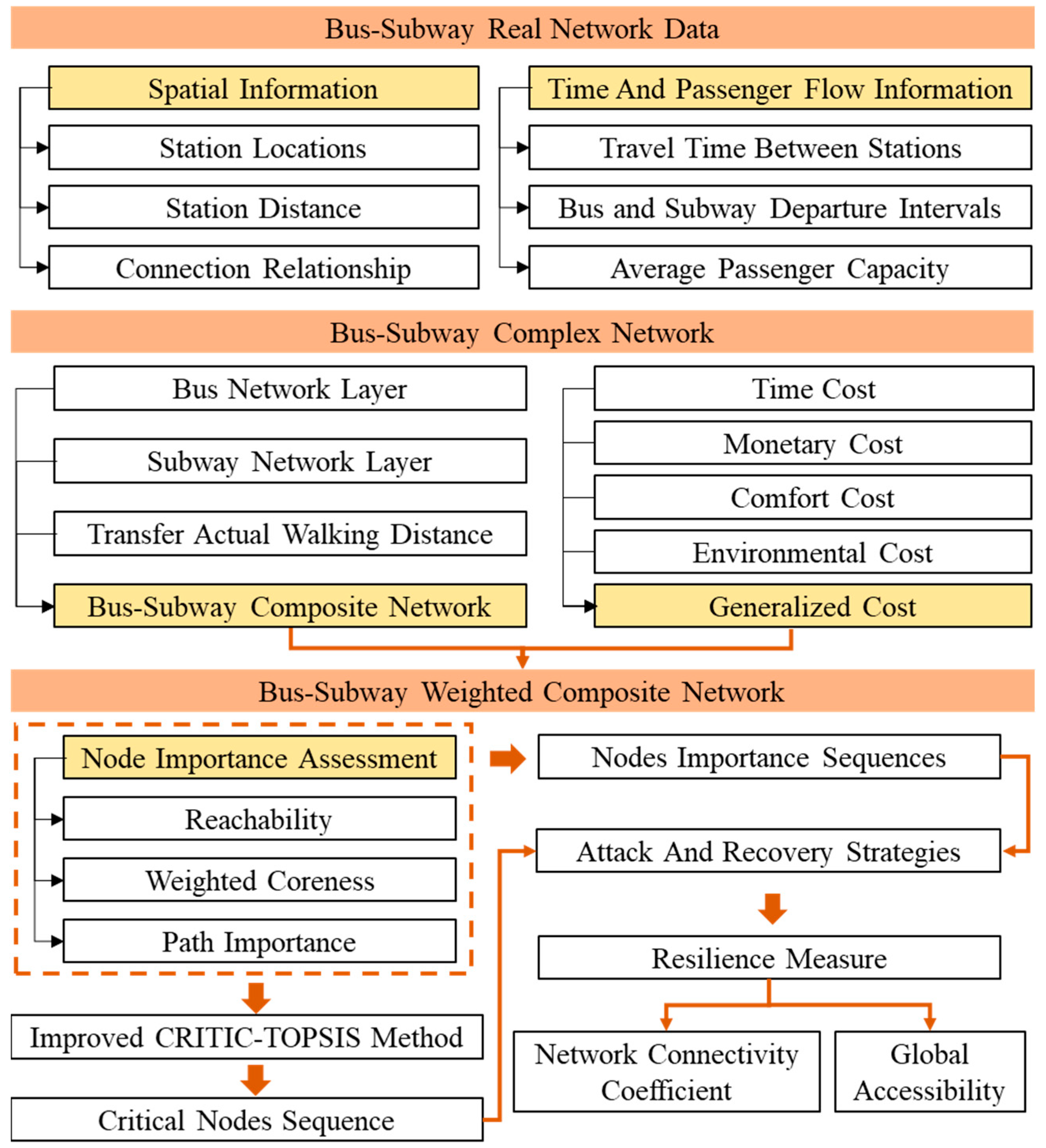
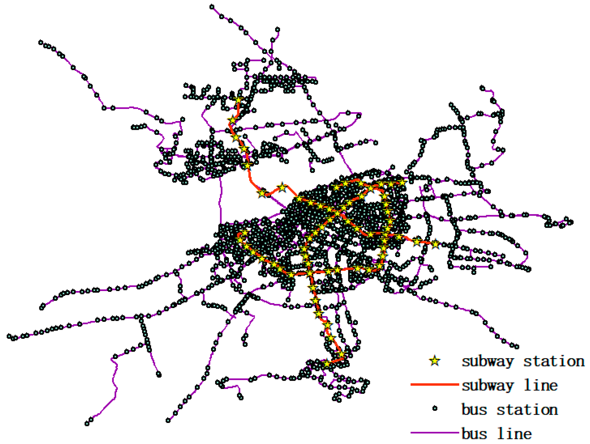
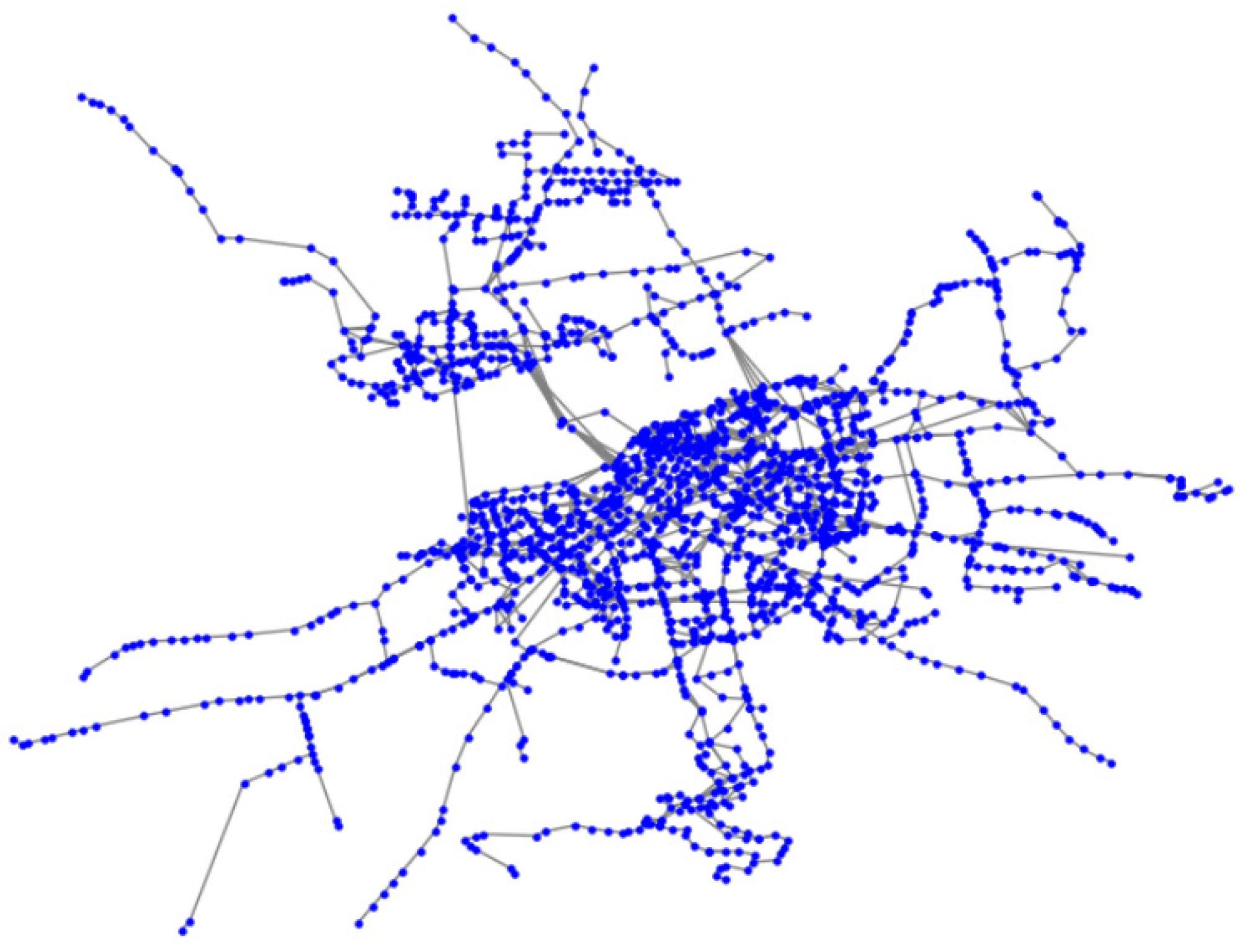
2. Construction of Weighted Composite Network

This study employs the generalized cost between nodes to assign weights to a network, and measures the resilience of this weighted bus–subway composite network. Initially, the connectivity between the nodes is characterized by computing the magnitude of the generalized cost between the nodes, and a bus–subway weighted network considering this generalized cost is established. Subsequently, the critical nodes sequence is identified through reachability, path importance, and weighted coreness, leading to the generation of four attack and recovery sequences. Finally, the resilience of the network under disturbance events is measured using the global accessibility and network connectivity coefficient. The process for measuring the resilience of this bus–subway weighted composite network is illustrated in Figure 1.

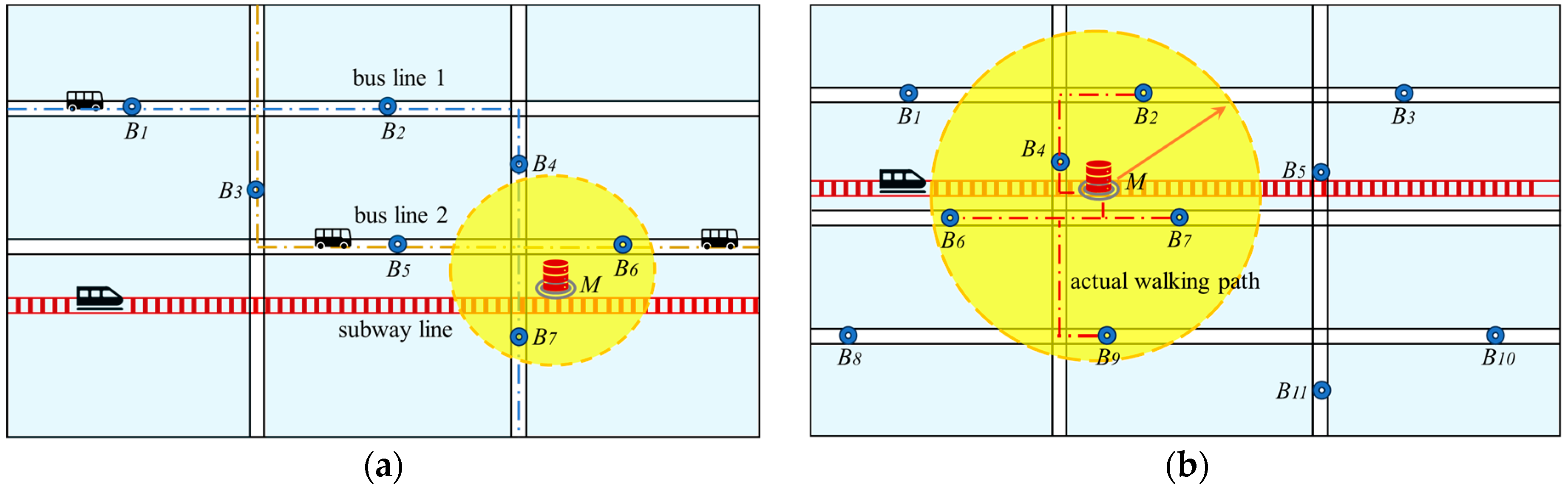
2.1. Construction of Unweighted Composite Network

The Space-L model, a space-based approach to constructing complex networks, is commonly employed to establish transportation network models [26]. It can not only reflect transportation elements, such as station connection relationships, geographical distances, and flow paths, but also be used to analyze the transportation network structure and spatial characteristics. Consequently, it holds significant relevance for the modeling and analysis of transportation systems.
Therefore, this study utilizes the Space-L model to abstract the stations as nodes and the segments between neighbor stations as edges. Specifically, the bus system is depicted as network G ( N b , E b ) , comprising bus stations and bus station segments. Given the bidirectional nature and shared up-and-down stations of buses and subways, an undirected complex network is formulated. Here, N b = { n 1 b , n 2 b , n 3 b , n n b } and E b = { e 1 b , e 2 b , e 3 b , e m b } denote the sets of bus stations and bus station segments, respectively, where n represents the total number of bus stations, and m indicates the total number of bus station segments. Similarly, the subway network is represented as network G ( N m , E m ) , with the subway station set and subway station segment set denoted by N m = { n 1 m , n 2 m , n 3 m , n n m } and A m = { e 1 m , e 2 m , e 3 m , e m m } , respectively. Through the above process, two single-layer networks are obtained: a bus network and a subway network.
In the actual travel process, there are often a large number of transfers between buses and subways, due to the connections between buses and subways, so it is necessary to establish a transfer connection between the two networks. Owing to the limitations of online map navigation data in the past, it was impossible to obtain walking navigation distances in batches. Previous research usually used the straight-line distance between subway stations and bus stations to determine whether there was a transfer [27]. This ignored the fact that there may be a huge gap between the straight-line distance and the actual walking distance. However, passengers are very sensitive to the transfer distance when transferring. Currently, Amap (a digital map developed by Alibaba and widely used for travel navigation in China) has opened up navigation data to researchers to obtain the actual distance of walking paths. Therefore, this study utilizes actual walking distances to determine whether there is a transfer, which will result in a more realistic transfer relationship compared to the straight-line distance. If the actual walking distance between a bus station and a subway station is within an acceptable range, a transfer edge is established between them. Otherwise, it is considered that no transfer exists between the bus stop and the subway station. The schematic diagram for determining the transfer relationship is displayed in Figure 2. The specific steps are as follows:
Step 1: Set the coverage area of subway stations with a radius of R, and define the acceptable walking distance as W, where R is 500 m and W is 500 m [28].
Step 2: Select any subway station n s m and utilize Amap API to retrieve the actual walking distance D ( n s m , n k b ) from all bus stations n k b to n s m within the coverage area.
Step 3: Verify the actual walking distance D ( n s m , n k b ) from bus station n k b to subway station n s m . If D ( n s m , n k b ) W , establish a transfer edge a s k mb between n s m and n k b .
Step 4: Repeat the process outlined in Step 3 to examine the actual walking distance between all bus stations and subway stations.
Step 5: Repeat the procedure described in Step 2, iterating through all subway stations to establish transfer connections.

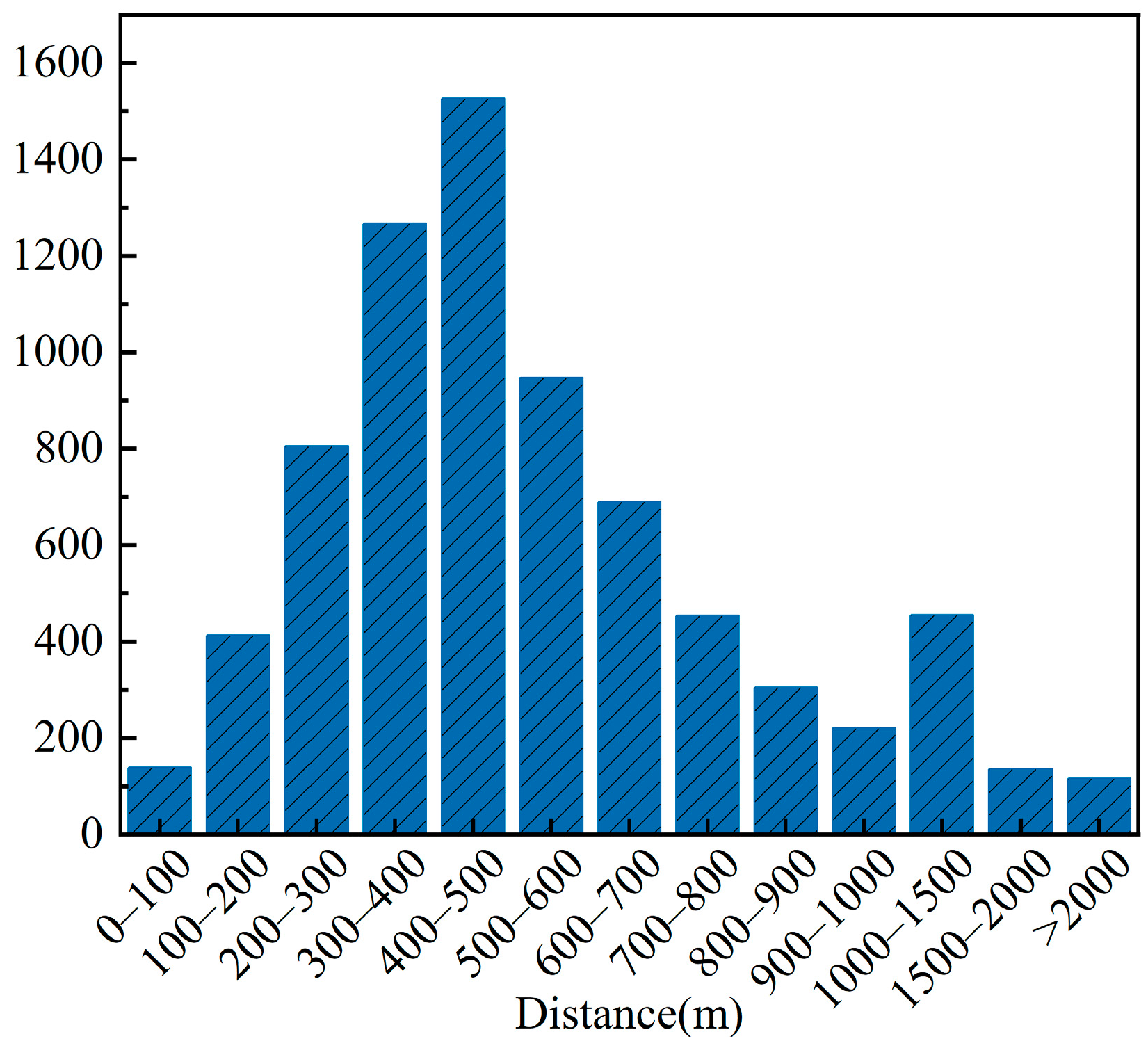
2.2. Generalized Cost-Weighting Method

The ease of passing through different stations varies greatly, which always affects the path choice of travelers [29]. But existing studies have often not considered it when measuring network resilience. In other words, it is unreasonable for them to view the composite network as an unweighted network or only use traffic to weight the network [30]. Residents consider various factors when traveling, such as comfort level, travel time, monetary cost, and safety. Therefore, this study comprehensively considers the travel time, fare, comfort, and environment factors when residents use buses and subways to travel. The network is weighted by applying the generalized cost, composed of the travel time, fare, comfort cost, and environmental cost as the weights. Moreover, the composite network composed of buses and subways is a space–time network. In addition to studying the spatial layout of the network, this study also considers the difference in departure frequency between buses and subways when studying two widely different networks: bus and subway. The generalized cost of station segment i is shown in Equation (1). It can be seen that the greater the generalized cost or the longer the departure interval, the more difficult it is to travel between stations.
F i = f E i
The generalized cost-weighting model for a bus or subway passing through station segment i is depicted in Equation (2).
E i = M i + T i + S i + U i
Regarding the monetary costs, this study calculates the average cost per kilometer of travel based on a survey of bus and subway fares. Then, multiplying this cost by the distance between stations yields the monetary cost of the distance traveled. The monetary cost of a bus or subway passing through station segment i is illustrated in Equation (3).
M i = η 1 l i
For the travel time cost, the travel time for buses can be retrieved by accessing the running time between neighbor stations through Amap API, while subway travel time can be calculated based on the time difference between neighbor stations using the arrival schedule. The travel time cost of a bus or subway passing through station segment i is presented in Equation (4).
T i = η 2 t i
The degree of crowding inside the carriage is a crucial factor influencing comfort. Therefore, this study calculates the comfort cost based on the level of crowding. The comfort cost of a bus or subway passing through station i is depicted in Equation (5).
S i = η 3 q c t i
Due to environmental threats and energy constraints, carbon emissions have attracted more and more attention. Therefore, this study calculates the environmental costs according to the carbon emissions during bus or subway operation. The calculation of the environmental cost is shown in Equation (6).
U i = η 4 l i μ
When applying the generalized cost to weight the network, it is necessary not only to compute the weights between bus stations and subway stations, but also to determine the costs associated with bus and subway transfer edges. As per the assumptions made during the construction of the composite network in Section 2.1, this study assumes that all transfers are conducted on foot. Hence, for the cost of transfer edge j, the actual walking distance of a passenger’s transfer can be obtained through Amap API. The actual walking distance is then divided by the average walking speed to calculate the walking time required for the transfer. Here, the average walking speed is assumed to be 1.2 m/s. The generalized cost of transfer edge j is formulated as shown in Equation (7).
F j = η 5 c j t j

3. Bus–Subway Weighted Network Characteristics

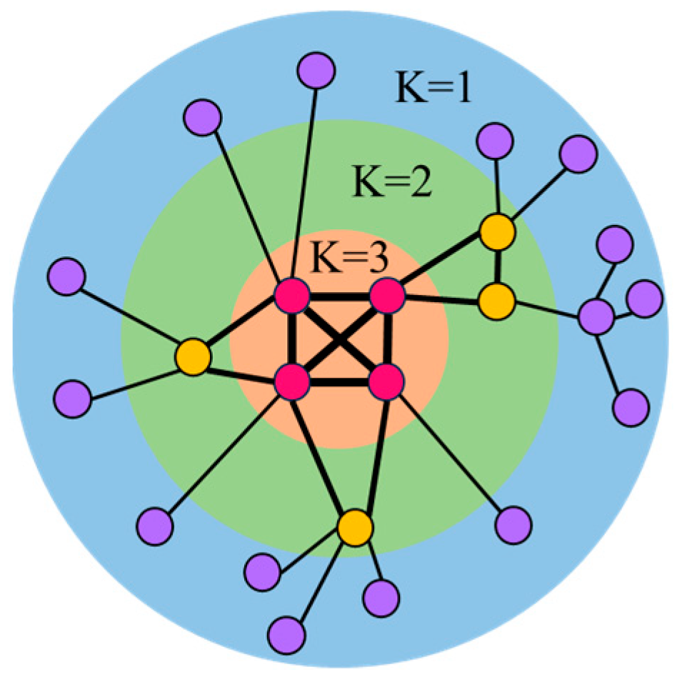
3.1. Node Importance Indicators

The node importance is an index for measuring the influence of the nodes within complex networks, and different types of node importance indicators provide various perspectives with which to evaluate the influence of the nodes. Through analyzing node importance, we can gain deeper insights into their roles and positions within the network, resulting in a better understanding of the spatial distribution characteristics of the important nodes in the network. Moreover, it provides a reference for identifying the critical nodes in the network. Hence, this study comprehensively examines the function and structure of the bus–subway composite network, employing three indicators—reachability, path importance, and weighted coreness—to conduct the importance analysis for the nodes within the network.
The reachability is defined as the reciprocal of the sum of the generalized cost from a node to other reachable nodes, which represents the overall ease of connectivity between the node and other reachable nodes. This indicator is more suitable for networks with good connectivity. In this study, we use this indicator to calculate the reachability of nodes when the network is not under attack. The higher the generalized cost for a node to reach other nodes, the more difficult it is to reach them, and the lower its reachability, tending towards zero. Conversely, the lower the generalized cost, the higher the reachability. The calculation of reachability is outlined in Equation (8).
C a ( v i ) = 1 j = 1 , i j N σ i j f i j
The path importance signifies the frequency that a node serves as the shortest path connecting different nodes in the network. In a generalized cost-weighted network, each station segment possesses a distinct generalized cost, and the smaller a path’s generalized cost, the higher the frequency of passing through the node, further indicating that the node has a stronger “hub” position in the network. The calculation of path importance is illustrated in Equation (9).
C b ( v i ) = 2 ε s t ( v i ) ( N 1 ) ( N 2 ) ε s t
To analyze the importance of the nodes in a network structure, the most commonly used method in related studies is degree centrality [31]. The degree centrality reflects the degree of the direct connection of a node in ae network, that is, how many direct connections a node has. The calculation of the degree centrality of a node is shown in Equation (10).
C d ( v i ) = k i N 1
While degree centrality can depict a node’s direct influence, research by Kitsak et al. indicated that highly influential nodes may also exhibit low degree centrality in a network [32]. These nodes often function as “bridge points”, as illustrated in Figure 3. Despite the low degree centrality of the red node in the figure, it is evident that the red node plays a significant bridging role. Therefore, this study introduces coreness to complement the node characteristics that degree centrality fails to capture.
The coreness of a node refers to the layer number within the largest core to which the node belongs [33,34]. It serves as an indicator to gauge the depth of a node within a network. Figure 4 illustrates the calculation method for node coreness. Initially, a threshold of K = 1 is set, and then all the nodes with a degree value of less than or equal to 1 in the network are removed. If the removal leads to the emergence of new nodes with a degree value of less than or equal to 1, they are continuously eliminated until the degree values of the remaining nodes in the network exceed 1. Subsequently, the coreness of these removed nodes is assigned as 1, hence the coreness of the nodes in the outermost circle of Figure 4 is 1. Similarly, by setting K = 2, 3, …, n, it is observed that the coreness of the nodes in the middle circle equals 2, while the coreness of the nodes in the innermost circle equals 3.
The coreness integrates the advantages of degree centrality but also compensates for its inability to identify “bridge points”. However, the traditional coreness calculation is based on degree values for layering, which cannot capture the weights of the edges between nodes, rendering it unsuitable for weighted networks. To address this issue, this study introduces the local strength indicator as a replacement for degree values, enhancing the traditional coreness calculation method to better suit the evaluation of node importance in weighted networks. The calculation of node local strength is shown in Equation (11).
C w = j = 1 , i j N 1 w i j

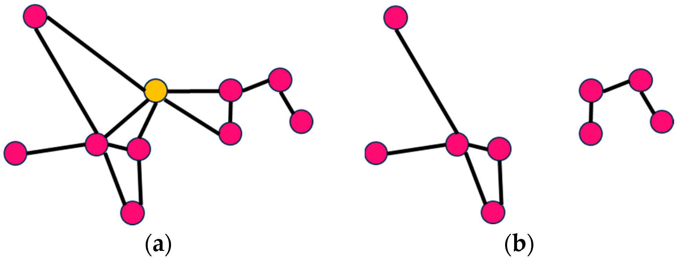
3.2. Identification of Critical Nodes

The critical nodes refer to the ones with high influence and importance in a network, whose breakdown often leads to large-scale network failures. Therefore, prioritizing their recovery can effectively enhance a network’s resilience. Based on the above nodes analysis and a comprehensive consideration of the three indicators (i.e., reachability, path importance, and weighted coreness), this study identifies the critical nodes in the bus–subway network using the improved CRITIC-TOPSIS method [35]. Compared to a single indicator approach, the critical nodes identified take into account the role of various indicators in the network, thus compensating for the shortcomings caused by the different focuses of single indicators.
There are many research methods for obtaining indicator weights and comparing schemes, such as the Best–Worst Method [36] and Fuzzy-TOPSIS [37]. However, these methods have their own limitations for critical nodes identification. Fuzzy-TOPSIS is suitable for determining the weights of factors with an uncertain scope and boundaries. In this study, the criteria are clearly defined, and we need a method to accurately determine the weights of the evaluation indicators using their precise values. The Best–Worst Method requires the decision makers to select the best and worst criteria based on experience and actual engineering needs. The accuracy of the Best–Worst Method depends on the decision makers’ ability to determine these criteria, which may introduce subjectivity and require a high level of expertise. This subjectivity may lead to biased or inconsistent results, especially in complex network analysis. CRITIC-TOPSIS is particularly useful for the multi-criteria decision-making scenario in this study because it can objectively determine the weights of the evaluation indicators based on contrast strength and correlation. Compared with other methods, CRITIC-TOPSIS reduces subjectivity and provides a robust assessment of the importance of the evaluation indicators.
The CRITIC method is an objective weighting technique that utilizes the comparative strength and conflict degree of the evaluation indicators to assign weights [38]. It comprehensively determines the indicator weights based on the comparative strength and conflict between the indicators, effectively merging both aspects into the weighting process. However, the traditional CRITIC method, as depicted in Equation (12), suffers from the drawback of being unable to reflect the degree of internal value discreteness of the indicators.
C j = σ j t = 1 n ( 1 r t j )       ( j = 1 , 2 , 3 n )
To address this, this study introduces information entropy to enhance the traditional CRITIC method. Information entropy serves as an indicator of numerical dispersion: the greater the dispersion, the higher the information entropy, and vice versa. This enhancement allows the improved CRITIC method to determine the weights based on the dispersion of the internal indicator values, while assessing the contrast intensity and conflict between the indicators, thus yielding more rational weight values. Additionally, the conflict between the indicators utilized in this study solely depends on their correlation. Therefore, as the correlation coefficient does not have negative values, the absolute value of the correlation coefficient is taken. The process of calculating weights using the improved CRITIC method is outlined below.
Assume there are m evaluation objects and n evaluation indicators in the original evaluation matrix. Subsequently, the weight data matrix P i j is constructed, and then the information entropy value of the j-th indicator is calculated, where k is a constant and k = 1/ln n.
e j = k i = 1 m P i j × ln P i j
Improvements are made to determine the indicator weights based on information entropy.
C j = e j t = 1 n ( 1 | r t j | )       ( j = 1 , 2 , 3 n )
W j = C j j = 1 n C j       ( j = 1 , 2 , 3 n )
The TOPSIS method is a multi-attribute decision-making method [39]. Its basic principle is to determine the best solution by comparing the similarity between each solution and the positive and negative ideal solutions. Based on the weights of the improved CRITIC method, the TOPSIS method is used to sort all the nodes. First, the weighted normalization matrix Z i j needs to be calculated based on the normalization matrix Y i j and the weights W j of each indicator. Secondly, the positive ideal solution B + and the negative ideal solution B are determined. Then, the Euclidean distance of each node to the positive ideal D i + and the negative ideal solution D i are calculated. Finally, the relative progress C i of each node is calculated according to Equation (16) to obtain the critical nodes sequence L G = s o r t [ C 1 , C 2 , C m ] .
C i = D i D i + + D i       ( i = 1 , 2 , , m )

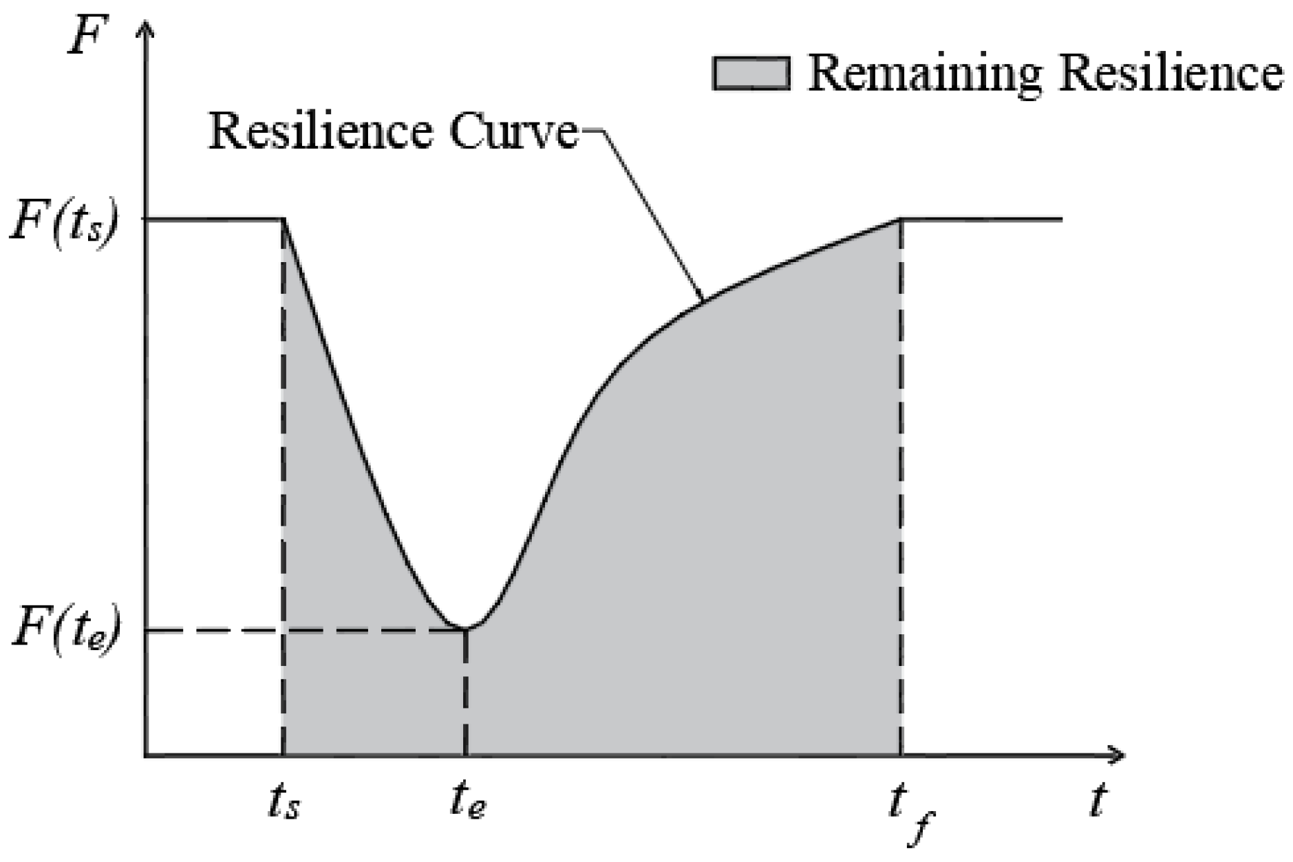
4. Resilience Measurement Model

This study simulates network attacks and recoveries based on real-world scenarios when public transportation encountered emergencies. When the network is under attack, the attacked stations and their edges are removed from the network, as illustrated in Figure 5. During the recovery process, the nodes are gradually reintroduced based on the original network’s connective relationship and a predetermined recovery sequence, with edges established between them, as depicted in Figure 6. Specifically, the attack methods include random attack and deliberate attack strategies, and the recovery methods also include random recovery and deliberate recovery strategies. Random attacks refer to the random selection of nodes in the network for removal, while deliberate attacks remove nodes in a certain sequence. Similarly, the recovery process follows analogous principles.
It is evident that a random attack and recovery are accidental and cannot reflect the essence of the security bottom line of a network’s resilience. Hence, this study constructs a deliberate attack and recovery strategy based on node reachability, path importance, weighted coreness, and the critical nodes sequence, and compares the resilience of the bus–subway weighted composite network under different attack and recovery strategies.
In previous studies, robustness and vulnerability have commonly been employed to measure the impact of disturbance events on a bus–subway composite network. While robustness and vulnerability effectively characterize a network’s response to attacks, they overlook the subsequent recovery process. Since the recovery process significantly influences the overall network performance, solely relying on robustness and vulnerability measurements fails to capture the complete impact of disturbance events on a network. Therefore, this study adopts resilience as a metric with which to measure the influence of sudden events on a network, aiming to describe the alterations in network performance throughout the whole period of the disturbance events.
The resilience of a bus–subway network refers to its capacity to absorb interference and rapidly recover network performance when facing disturbance events during operation. As depicted in Figure 7, at time t s , a disturbance event occurs and the network begins to be attacked. As the attack persists, network performance steadily declines. It is not until time t e , when the attack concludes, that the network’s recovery work begins. With continuous repairs, the network’s resilience gradually increases until it achieves full recovery at time t f . The area under the resilience curve from the beginning of the attack to the conclusion of recovery represents the network’s resilience throughout the entire disturbance event. Unlike robustness and vulnerability, the resilience measurement emphasizes the integral performance changes in the network throughout the disturbance event. In today’s intricate traffic environment, it can better inform the pre-disaster allocation of security resources and post-disaster emergency strategy formulation, enhancing the sustainability and adaptability of the public transportation system. Based on the aforementioned theories, the specific calculation of resilience is illustrated in Equation (17).
R ( t ) = t s t F ( t ) d t ( t t s ) F ( t s )
The connectivity and accessibility are two crucial performance metrics of a network. The connectivity indicates the number of nodes in a network that can be traversed, while the accessibility reflects the ease of traversal between passable nodes. To expound the changes in network connectivity and accessibility during the attack and recovery phases, this study employs two metrics—the network connectivity coefficient and global accessibility—to describe the network’s resilience.
The calculation of the network connectivity coefficient is shown in Equation (18).
S = 1 θ i = 1 θ T i T
The calculation of global accessibility is presented in Equation (19).
E = i j N 1 f i j

5. Results and Discussion

This study takes the weighted composite network composed of buses and subways in Harbin as an example with which to analyze a weighted composite network and measure its resilience. The study area is the main urban area of Harbin and its suburbs, including seven counties and districts: Daoli, Daowai, Nangang, Xiangfang, Pingfang, Songbei, and Hulan. There are 209 regular bus lines, 6182 bus stations, 3 subway lines, and 65 subway stations in the study area. This study visualizes the composite network composed of buses and subways in Harbin based on the line name, station name, station coordinates, station spacing, and other information obtained from Amap API. Its real layout is shown in Figure 8.
Table 2 provides the operating information for the bus and subway lines in the study area, including the line type, departure interval, vehicle rated passenger capacity, and average passenger capacity. The departure intervals used in this study are the departure intervals during morning peak hours on weekdays.
Table 3 offers the coordinates and connection relationships of the front and back stations, station distances, station running times, generalized cost, and other information required to build a bus–subway weighted composite network. The running times and distances of the bus station sections are obtained from Amap API, the running times of the subway station sections are obtained from the subway timetable, and the distances between the stations are obtained from map measurements.
According to the survey results for the operation status of buses and subways, it can be seen that the cost of traveling by bus or subway is 0.25 CNY/km; thus, the operating monetary cost coefficient η 1 is 0.25. The average salary level of the people participating in the survey is about CNY 6300. Calculating based on 8 h of work per day, the cost per minute per person is about CNY 0.31, so the travel time value coefficient η 2 is 0.31. In addition, the crowding value coefficient η 3 is 0.2045 [40], and the value coefficient of carbon trading η 4 is 0.06 [41]. The carbon emissions from the electricity consumed by the buses per kilometer are 0.804 kgCO2/km, and the carbon emissions from the electricity consumed by the subways per kilometer are 1.479 kgCO2/km. We assume that the number of passengers transferring at transfer stations is 30% of the average passenger capacity divided by the number of stations.
The time and distance distributions between stations are given in Figure 9 and Figure 10. It can be seen that the time between stations is mainly concentrated in the range of 1 to 3 min, and the distance is mainly concentrated in the range of 200 to 700 m.
In order to more clearly display the importance of the stations and the connection relationships within the network, this study merges stations with the same name. After this merging process, the topological network consists of 1892 nodes and 3201 edges. Subsequently, weights are added to the edges based on the generalized cost between nodes, transforming the unweighted network into a weighted network. Figure 11 presents the topology diagram of the composite network. It can be observed that the topological structure of the composite network is essentially the same as the real network form, although the number and density of nodes are reduced due to the merging of stations with the same name. In addition, since there are multiple bus nodes within the pedestrian walking tolerance range within the coverage area of a subway station, connections are established between them, which significantly increases the number of connections between subway nodes.
To understand the status of the initial network, Table 4 presents the characteristics of Harbin’s bus weighted network and the bus–subway composite weighted network. It can be observed that the composite network outperforms the single network, with the maximum connected subgraph increasing by 3.56% and the weighted network efficiency improving by 5.26%. This improvement is attributed to the higher operational speed of the subway compared to the bus, which reduces the generalized cost and alters the shortest path between nodes. Consequently, the integration of subway stations into the bus network significantly enhances network efficiency.
After calculation, the impact of the comfort cost and environmental cost on the generalized cost is less than 15%. The generalized cost is mainly influenced by the monetary cost and time cost. Therefore, we next conduct a sensitivity analysis on the operating monetary cost coefficient η 1 and the travel time value coefficient η 2 .
While keeping the other variables unchanged, Figure 12a lists the changes in the weighted network efficiency when A is 0.15, 0.20, 0.25, 0.30, and 0.35, respectively. Figure 12b lists the changes in the weighted network efficiency when B is 0.21, 0.26, 0.31, 0.36, and 0.41, respectively.
The results show that as the coefficient values increase or decrease, network efficiency tends to stabilize. This may be because when the coefficient values increase, the corresponding cost accounts for a larger proportion of the generalized cost, making it the main factor affecting the shortest path. At the same time, increasing the cost of each section does not change the shortest path. Conversely, as the values decrease, its proportion of the generalized cost decreases, and the choice of the shortest path is mainly influenced by other costs.
According to Equations (8) to (11), Python is used to calculate the reachability, path importance, and weighted coreness of each node in the weighted network. To reveal the spatial distribution patterns of node importance under different evaluation indicators, Figure 13 presents the visualization results for the importance of each node. It is evident that there are significant differences in the spatial distribution of the important nodes identified using various evaluation indicators. The distributions of reachability and weighted coreness exhibit central agglomeration, with centrality decreasing from the urban center to the periphery. This trend likely arises because bus stations in the city center are denser, the distances between stations are shorter, and the nodes are more closely interconnected, leading to deeper node hierarchies, higher loads, and stronger connections with other highly central nodes.
Conversely, in the distribution of path importance, important and non-important nodes are interspersed without clear aggregation characteristics. Nonetheless, it is apparent that the important nodes are concentrated along subway lines. This concentration is due to the subway transit’s shorter departure intervals and faster speeds compared to conventional buses, resulting in a lower generalized cost. These indicators assess node importance from different perspectives, reflecting the characteristics of the nodes based on various focuses and physical meanings, and they will serve as a crucial basis for identifying the critical nodes within the network.
In addition, it is worth noting that there are also huge differences in the sequences of the top-20 most important nodes under the different evaluation indicators. Even though the reachability and weighted core degrees are similar in their spatial distributions, the number of repetitions among the top-20 most important nodes is not high. According to the sequences of the top-20 nodes under the different evaluation indicators given in Table 5, it can be seen that there are only three common nodes: 37, 40, and 1842. On the whole, except for 188, 85, and 316, the critical nodes identified in this study, based on the improved CRITIC-TOPSIS, are all nodes in the top 20 of other important indicators. The effectiveness of the weighted network critical node identification method proposed in this study is proved by this case.
Based on the sequences of the different nodes, multiple attack and repair strategies can be generated. We assume that when the network is disturbed, nodes are removed sequentially and are then restored after all the nodes have been removed. This study compares and analyzes the changes in the network connectivity coefficient and global accessibility under different attack and recovery strategies.
Figure 14 and Figure 15 show the network connectivity coefficient and global accessibility change curves under different attack and recovery sequences, respectively. The network is attacked and restored in different ways, resulting in large differences in network performance. Specifically, it can be seen from Figure 14a,b that during the attack process when the top 10% of the nodes in the path importance sequence are removed, the network connectivity coefficient curve decreases the fastest, with a decrease of 42.3%. When the first 20% of the nodes in the critical nodes sequence are removed, less than 10% of the nodes can be connected. This is due to the structural characteristics of complex networks. A few nodes play a pivotal role in the network. Once these nodes are removed, large areas of the network will fail. In the recovery process, if the critical nodes sequence is used for recovery, the curve will rise the fastest; if the recovery is based on the reachability, the curve will rise the slowest.
As can be seen from Figure 15a,b, the global accessibility is most sensitive to attacks on the critical nodes sequences. If the top 20% of the nodes in this sequence are removed, the network is on the verge of failure. During the network recovery process, the critical nodes sequence recovery curve and the path importance recovery curve rise the fastest. When the first 70% of the nodes are restored, the network is basically fully restored.
Figure 14 and Figure 15 provide further insights. Regardless of the method used to remove the first 60% of the nodes, both the network connectivity coefficient and global accessibility drop to less than 10%, indicating a near collapse of network performance. In contrast, the recovery curves vary significantly. Different restoration sequences exert diverse impacts on network performance. However, when employing the critical nodes sequence for restoration, the network’s connectivity coefficient and global accessibility are nearly fully restored after recovering the first 70% of the nodes.
It can be seen from Figure 7 that the network’s resilience under different attack and recovery strategies is measured by calculating the area enclosed by the resilience curve and the x-axis. In order to compare the resilience under different attack and recovery strategies, Table 6 gives the network connectivity coefficient and global accessibility resilience values under different attack and recovery sequences.
The network resilience value is defined as the average of the sum of the remaining performance of the network during the attack process and the increased performance of the network during the recovery process. During the attack process, a smaller remaining resilience value indicates more significant network failures. Conversely, during the recovery process, a greater increase in resilience value signifies a more effective network recovery.
In the attack process, the remaining network performance is minimized when the critical nodes sequence is followed, and maximized when the reachability sequence is followed. And in the recovery process, the network performance increase is maximized for the critical nodes sequence and minimized for the reachability sequence. This indicates that the recovery effect, in terms of both the network’s connectivity coefficient and global accessibility, is optimal when following the critical nodes sequence.
Based on the above analysis of the curves and the comparison of the resilience values, it can be concluded that for the nodes in the path importance sequence and critical nodes sequence, protective measures should be taken and emergency support resources should be allocated to them first. At the same time, when recovery begins, the identified critical nodes should be prioritized for repair and recovery. Therefore, this study provides an important reference for the allocation of supportive resources within public transportation systems before a disaster strikes and the formulation of post-disaster recovery strategies.
To compare the resilience of composite networks and single networks, Table 7 shows the resilience values for the network connectivity coefficient and global accessibility of bus–subway networks and bus networks under different attack and recovery sequences. It can be seen that the bus–subway network resilience value is generally higher than the bus network resilience value. However, the maximum increase (path importance sequence) is only 3.53%, which is not obvious. This is mainly due to the fact that Harbin has few subway lines, has not yet formed a mature network, and the subway is not deeply coupled with the bus network.

6. Conclusions

This study constructs a bus–subway composite network based on the Space-L model and the actual transfer distances for pedestrians. Subsequently, the network is weighted using the generalized cost between nodes. Then, the improved CRITIC-TOPSIS method is employed to integrate three node importance indicators—reachability, path importance, and weighted coreness—to identify the critical nodes. Finally, the network is attacked and restored based on the node importance sequence and critical nodes sequence, and the network resilience under the different sequences is compared. The main conclusions of this study are as follows:
(1)
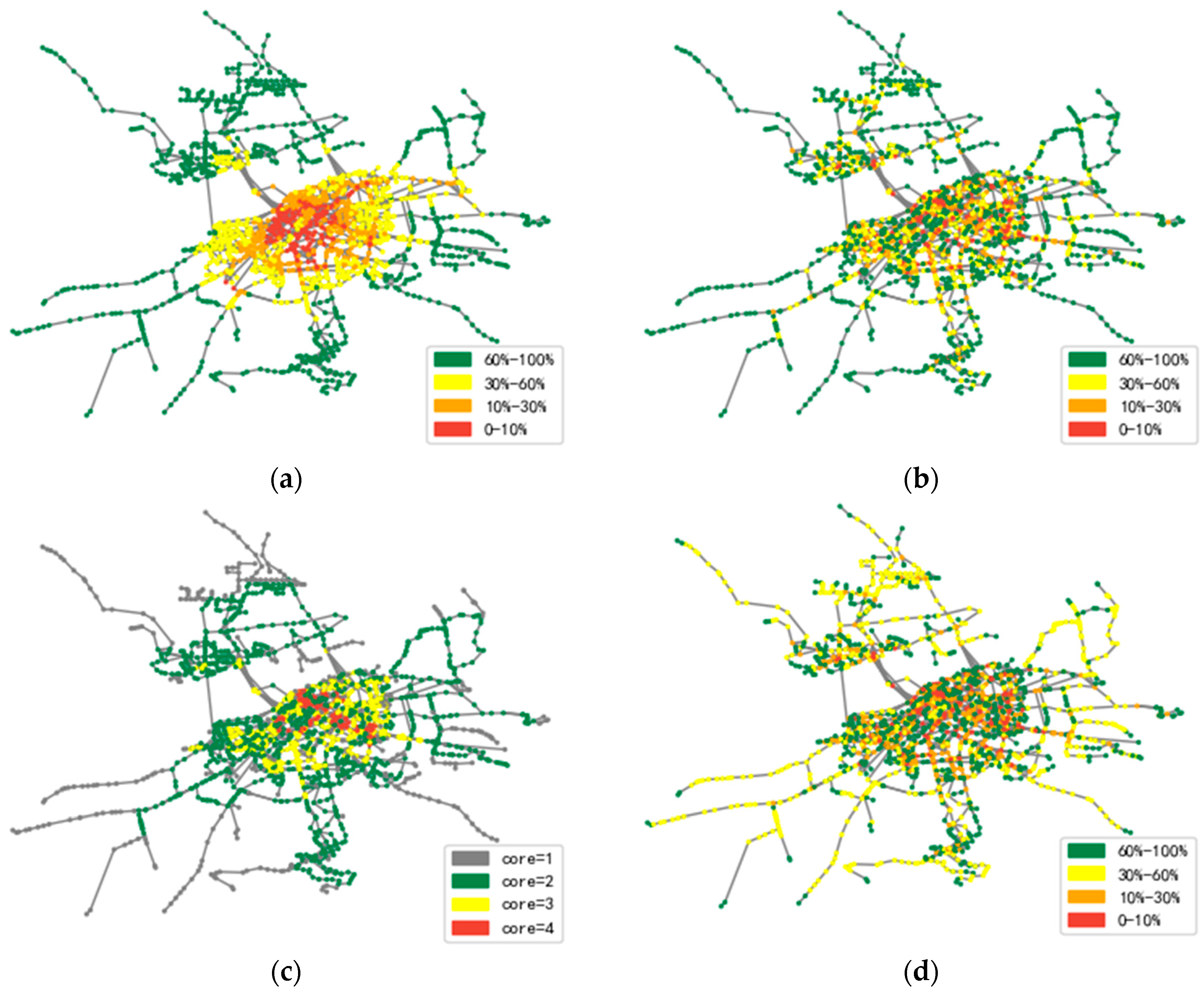
The importance of the nodes under the different evaluation indicators present different spatial distributions. The reachability and weighted coreness distribution of the nodes demonstrate central agglomeration, and their importance decreases from the urban center to the periphery. Conversely, in terms of the path importance distribution of the nodes, the nodes of high importance are staggered with nodes of low importance, lacking a discernible aggregation feature. These indicators reflect the characteristics of the nodes from different focuses, providing a basis for comprehensively identifying the critical nodes in the network.
(2)
There are distinct differences in the nodes with strong centrality identified by the different evaluation indicators. The top-20 nodes for the three indicators of reachability, path importance, and weighted coreness have only three nodes in common. Even so, except for 188, 85, and 316, the top-20 critical nodes identified according to the improved CRITIC-TOPSIS method are all the top 20 nodes for the other importance indicators. This indicates that the identified critical nodes also have strong importance, which also illustrates the effectiveness of the critical nodes identification method used in this study.
(3)
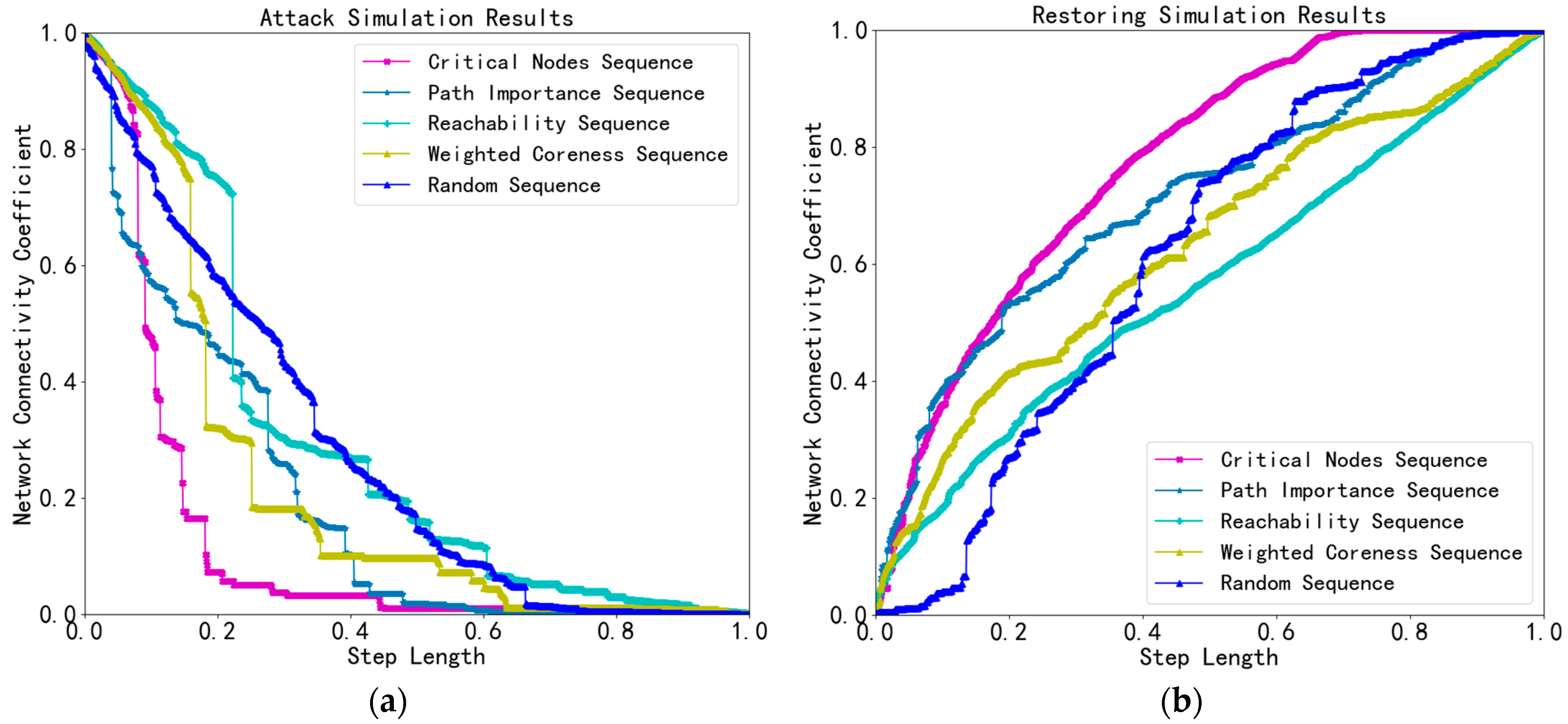
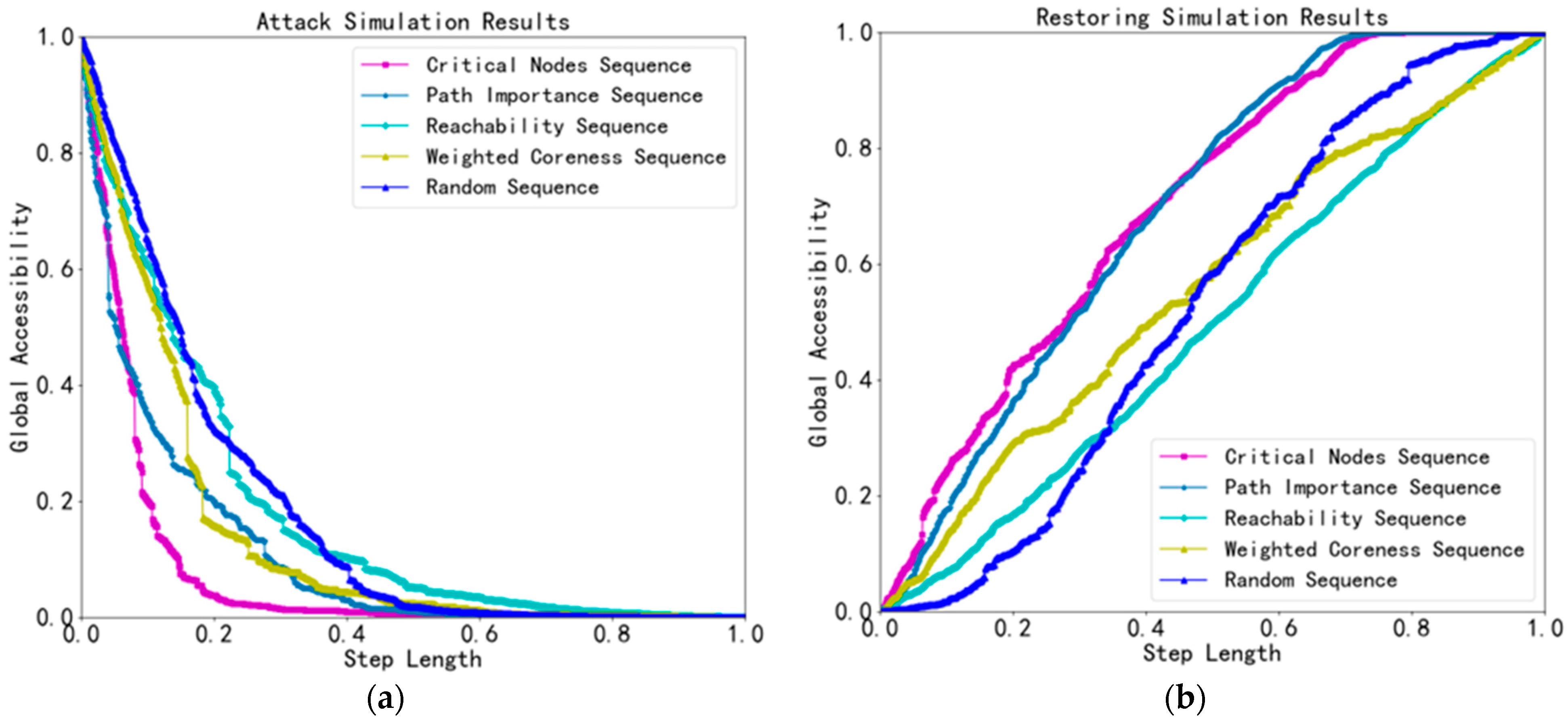
During the attack process, the network connectivity coefficient is most sensitive to attacks on the path importance sequence. When the first 10% of the nodes in this sequence are removed, the network connectivity coefficient declines the most rapidly, decreasing by 42.3%. And the global accessibility is most sensitive to attacks on the critical nodes sequence. When the top 20% of the nodes in this sequence are removed, the network is on the verge of failure. During the recovery process, both the network connectivity coefficient and global accessibility recover most effectively when following the critical nodes sequence. When the first 70% of the nodes are restored, the network is nearly fully recovered. This study provides a crucial reference for allocating support resources within public transportation systems prior to a disaster and for developing recovery strategies post-disaster.
(4)
The overall performance of the bus–subway composite network surpasses that of the single bus network. The maximum connected subgraph and weighted network efficiency of the initial network are increased by 3.56% and 5.26%, respectively. Additionally, after undergoing attack and recovery, the resilience of the bus–subway composite network remains higher than that of the single bus network. However, the improvement is not obvious, with the maximum increase being only 3.53%.
Compared with the classic network performance metrics under perturbations, this study uses resilience instead of robustness, which considers the entire process of disruption. It is worth noting that this study employs actual walking distances instead of Euclidean distances when constructing the composite network, and calculates the generalized cost between nodes to weight the network. There are several research questions that can be built upon this work. Please note that in Section 4, “Resilience Measurement Model”, we perform attacks and recoveries based on various node importance sequences. We are currently working on incorporating cascading failures into the attack process. Additionally, this study identifies the spatial distribution characteristics of node importance. We will also analyze more cities with different network topologies to observe the impact of network topology on the spatial distribution of nodes.

Author Contributions

Methodology, funding acquisition, and writing—original draft preparation, Y.P.; software and visualization, F.X.; investigation and data curation, Z.W.; writing—review and editing, C.D. All authors have read and agreed to the published version of the manuscript.

Funding

This research was funded by the Key Program of the National Natural Science Foundation of China (grant number 51638004) and the National Natural Science Foundation of China (grant number 71771047).

Data Availability Statement

Restrictions apply to the availability of these data. Data were obtained from Amap (a digital map developed by Alibaba and widely used for travel navigation in China) and are available at https://lbs.amap.com/api/webservice/summary (accessed on 18 October 2023) with the permission of Amap.

Acknowledgments

The authors acknowledge all of the team members of the Transportation Research Center of Northeast Forestry University for their insightful comments, which significantly improved the quality of the analysis and presentation of this study.

Conflicts of Interest

The authors declare no conflicts of interest.

References

  1. Dong, S.; Mostafizi, A.; Wang, H.; Gao, J.; Li, X. Measuring the Topological Robustness of Transportation Networks to Disaster-Induced Failures: A Percolation Approach. J. Infrastruct. Syst. 2020, 26, 04020009. [Google Scholar] [CrossRef]
  2. Oehlers, M.; Fabian, B. Graph Metrics for Network Robustness—A Survey. Mathematics 2021, 9, 895. [Google Scholar] [CrossRef]
  3. Abdelaty, H.; Mohamed, M.; Ezzeldin, M.; El-Dakhakhni, W. Quantifying and Classifying the Robustness of Bus Transit Networks. Transp. A Transp. Sci. 2020, 16, 1176–1216. [Google Scholar] [CrossRef]
  4. Zhang, Y.; Ng, S.T. Robustness of Urban Railway Networks against the Cascading Failures Induced by the Fluctuation of Passenger Flow. Reliab. Eng. Syst. Saf. 2022, 219, 108227. [Google Scholar] [CrossRef]
  5. Abdelaty, H.; Mohamed, M.; Ezzeldin, M.; El-Dakhakhni, W. Temporal Robustness Assessment Framework for City-Scale Bus Transit Networks. Phys. Stat. Mech. Appl. 2022, 606, 128077. [Google Scholar] [CrossRef]
  6. Jiang, J.; Wu, L.; Yu, J.; Wang, M.; Kong, H.; Zhang, Z.; Wang, J. Robustness of Bilayer Railway-Aviation Transportation Network Considering Discrete Cross-Layer Traffic Flow Assignment. Transp. Res. Part D Transp. Environ. 2024, 127, 104071. [Google Scholar] [CrossRef]
  7. El-Rashidy, R.A.; Grant-Muller, S.M. An Assessment Method for Highway Network Vulnerability. J. Transp. Geogr. 2014, 34, 34–43. [Google Scholar] [CrossRef]
  8. Shen, Y.; Yang, H.; Ren, G.; Ran, B. Model Cascading Overload Failure and Dynamic Vulnerability Analysis of Facility Network of Metro Station. Reliab. Eng. Syst. Saf. 2024, 242, 109711. [Google Scholar] [CrossRef]
  9. Zhang, J.; Wang, S.; Wang, X. Comparison Analysis on Vulnerability of Metro Networks Based on Complex Network. Phys. Stat. Mech. Appl. 2018, 496, 72–78. [Google Scholar] [CrossRef]
  10. Sun, Y.; Xie, B.; Wang, S.; Wu, D. Dynamic Assessment of Road Network Vulnerability Based on Cell Transmission Model. J. Adv. Transp. 2021, 2021, 5575537. [Google Scholar] [CrossRef]
  11. Wang, Y.; Wang, L.; Liu, Z. Vulnerability Metrics of Multimodal Composite Transportation Network. J. Traffic Transp. Eng. 2023, 23, 195–207. [Google Scholar]
  12. Gu, Y.; Fu, X.; Liu, Z.; Xu, X.; Chen, A. Performance of Transportation Network under Perturbations: Reliability, Vulnerability, and Resilience. Transp. Res. Part E Logist. Transp. Rev. 2020, 133, 101809. [Google Scholar] [CrossRef]
  13. Zhang, J.; Ren, G.; Song, J. Resilience-Based Restoration Sequence Optimization for Metro Networks: A Case Study in China. J. Adv. Transp. 2022, 2022, 8595356. [Google Scholar] [CrossRef]
  14. D’Lima, M.; Medda, F. A New Measure of Resilience: An Application to the London Underground. Transp. Res. Part A Policy Pract. 2015, 81, 35–46. [Google Scholar] [CrossRef]
  15. Dong, S.; Gao, X.; Mostafavi, A.; Gao, J.; Gangwal, U. Characterizing Resilience of Flood-Disrupted Dynamic Transportation Network through the Lens of Link Reliability and Stability. Reliab. Eng. Syst. Saf. 2023, 232, 109071. [Google Scholar] [CrossRef]
  16. Testa, A.C.; Furtado, M.N.; Alipour, A. Resilience of Coastal Transportation Networks Faced with Extreme Climatic Events. Transp. Res. Rec. 2015, 2532, 29–36. [Google Scholar] [CrossRef]
  17. Zhang, D.; Du, F.; Huang, H.; Zhang, F.; Ayyub, B.M.; Beer, M. Resiliency Assessment of Urban Rail Transit Networks: Shanghai Metro as an Example. Saf. Sci. 2018, 106, 230–243. [Google Scholar] [CrossRef]
  18. Aydin, N.Y.; Duzgun, H.S.; Wenzel, F.; Heinimann, H.R. Integration of Stress Testing with Graph Theory to Assess the Resilience of Urban Road Networks under Seismic Hazards. Nat. Hazards 2018, 91, 37–68. [Google Scholar] [CrossRef]
  19. Yin, K.; Wu, J.; Wang, W.; Lee, D.-H.; Wei, Y. An Integrated Resilience Assessment Model of Urban Transportation Network: A Case Study of 40 Cities in China. Transp. Res. Part A Policy Pract. 2023, 173, 103687. [Google Scholar] [CrossRef]
  20. Elmezain, M.; Othman, E.A.; Ibrahim, H.M. Temporal Degree-Degree and Closeness-Closeness: A New Centrality Metrics for Social Network Analysis. Mathematics 2021, 9, 2850. [Google Scholar] [CrossRef]
  21. Huang, L.; Huang, H.; Wang, Y. Resilience Analysis of Traffic Network under Emergencies: A Case Study of Bus Transit Network. Appl. Sci. 2023, 13, 8835. [Google Scholar] [CrossRef]
  22. Koopmans, C.; Groot, W.; Warffemius, P.; Annema, J.A.; Hoogendoorn-Lanser, S. Measuring Generalised Transport Costs as an Indicator of Accessibility Changes over Time. Transp. Policy 2013, 29, 154–159. [Google Scholar] [CrossRef]
  23. Santos, T.A.; Martins, P.; Soares, C.G. The Impact of Container Terminal Relocation on Hinterland Geography. J. Transp. Geogr. 2021, 92, 103014. [Google Scholar] [CrossRef]
  24. Tian, Z.; Sun, G.; Chen, D.; Qiu, Z.; Ma, Y. Method for Determining the Valid Travel Route of Railways Based on Generalised Cost under the Syncretic Railway Network. J. Adv. Transp. 2020, 2020, 8287648. [Google Scholar] [CrossRef]
  25. Super Transportation Network Demand and Forecast Technology Based on Multi-Mode Generalized Cost Model (Topic)—1—All Databases. Available online: https://webofscience.clarivate.cn/wos/alldb/summary/d9f51be7-6d3c-41cd-aa5d-425afbf1e114-f1dc01a8/relevance/1 (accessed on 6 June 2024).
  26. Xu, L.; Su, F.; Zhang, J.; Zhang, N. High-Speed Rail Network Structural Characteristics and Evolution in China. Mathematics 2022, 10, 3318. [Google Scholar] [CrossRef]
  27. Jun, M.-J.; Choi, K.; Jeong, J.-E.; Kwon, K.-H.; Kim, H.-J. Land Use Characteristics of Subway Catchment Areas and Their Influence on Subway Ridership in Seoul. J. Transp. Geogr. 2015, 48, 30–40. [Google Scholar] [CrossRef]
  28. Chen, C.; Wang, S.; Zhang, J.; Gu, X. Modeling the Vulnerability and Resilience of Interdependent Transportation Networks under Multiple Disruptions. J. Infrastruct. Syst. 2023, 29, 04022043. [Google Scholar] [CrossRef]
  29. Cao, Q.; Deng, Y.; Ren, G.; Liu, Y.; Li, D.; Song, Y.; Qu, X. Jointly Estimating the Most Likely Driving Paths and Destination Locations with Incomplete Vehicular Trajectory Data. Transp. Res. Part C Emerg. Technol. 2023, 155, 104283. [Google Scholar] [CrossRef]
  30. Ma, F.; Ao, Y.; Wang, X.; He, H.; Liu, Q.; Yang, D.; Gou, H. Assessing and Enhancing Urban Road Network Resilience under Rainstorm Waterlogging Disasters. Transp. Res. Part D Transp. Environ. 2023, 123, 103928. [Google Scholar] [CrossRef]
  31. Shen, J.; Zong, H. Identification of Critical Transportation Cities in the Multimodal Transportation Network of China. Phys. Stat. Mech. Appl. 2023, 628, 129174. [Google Scholar] [CrossRef]
  32. Kitsak, M.; Gallos, L.K.; Havlin, S.; Liljeros, F.; Muchnik, L.; Stanley, H.E.; Makse, H.A. Identification of Influential Spreaders in Complex Networks. Nat. Phys. 2010, 6, 888–893. [Google Scholar] [CrossRef]
  33. Lue, L.; Zhou, T.; Zhang, Q.-M.; Stanley, H.E. The H-Index of a Network Node and Its Relation to Degree and Coreness. Nat. Commun. 2016, 7, 10168. [Google Scholar] [CrossRef] [PubMed]
  34. Bae, J.; Kim, S. Identifying and Ranking Influential Spreaders in Complex Networks by Neighborhood Coreness. Phys. Stat. Mech. Appl. 2014, 395, 549–559. [Google Scholar] [CrossRef]
  35. Han, S.; Wang, B.; Ao, Y.; Bahmani, H.; Chai, B. The Coupling and Coordination Degree of Urban Resilience System: A Case Study of the Chengdu-Chongqing Urban Agglomeration. Environ. Impact Assess. Rev. 2023, 101, 107145. [Google Scholar] [CrossRef]
  36. Rezaei, J. Best-Worst Multi-Criteria Decision-Making Method: Some Properties and a Linear Model. Omega Int. J. Manag. Sci. 2016, 64, 126–130. [Google Scholar] [CrossRef]
  37. Akram, M.; Dudek, W.A.; Ilyas, F. Group Decision-Making Based on Pythagorean Fuzzy TOPSIS Method. Int. J. Intell. Syst. 2019, 34, 1455–1475. [Google Scholar] [CrossRef]
  38. Huang, S.-W.; Liou, J.J.H.; Chuang, H.-H.; Tzeng, G.-H. Using a Modified VIKOR Technique for Evaluating and Improving the National Healthcare System Quality. Mathematics 2021, 9, 1349. [Google Scholar] [CrossRef]
  39. Rao, C.; Gao, Y. Evaluation Mechanism Design for the Development Level of Urban-Rural Integration Based on an Improved TOPSIS Method. Mathematics 2022, 10, 380. [Google Scholar] [CrossRef]
  40. Zhu, J.-X.; Luo, Q.-Y.; Guan, X.-Y.; Yang, J.-L.; Bing, X. A Traffic Assignment Approach for Multi-Modal Transportation Networks Considering Capacity Constraints and Route Correlations. IEEE Access 2020, 8, 158862–158874. [Google Scholar] [CrossRef]
  41. Lin, H.; Tang, C. Analysis and Optimization of Urban Public Transport Lines Based on Multiobjective Adaptive Particle Swarm Optimization. IEEE Trans. Intell. Transp. Syst. 2022, 23, 16786–16798. [Google Scholar] [CrossRef]
Figure 1. Process for measuring resilience of bus–subway weighted composite networks.
Mathematics 12 02191 g001
Figure 2. Methodology for constructing bus–subway transfer edges. (a) Schematic representation of subway station coverage area. (b) Acquisition of shortest walking distance from bus stations to subway stations.
Mathematics 12 02191 g002
Figure 3. Schematic representation of a node with low degree value but high coreness.
Mathematics 12 02191 g003
Figure 4. Schematic illustration of coreness calculation.
Mathematics 12 02191 g004
Figure 5. Schematic representation of the network attack process. (a) Network before the attack. (b) Network after the attack.
Mathematics 12 02191 g005
Figure 6. Network recovery process diagram. (a) Network before the recovery. (b) Network during the recovery. (c) Network after the recovery.
Mathematics 12 02191 g006
Figure 7. Schematic diagram of toughness change curve.
Mathematics 12 02191 g007
Figure 8. Harbin bus–subway real network.
Mathematics 12 02191 g008
Figure 9. Time distribution between stations.
Mathematics 12 02191 g009
Figure 10. Distance distribution between stations.
Mathematics 12 02191 g010
Figure 11. Harbin city bus–subway topological network.
Mathematics 12 02191 g011
Figure 12. A sensitivity analysis of the weighted network efficiency. (a) The impact of the operating monetary cost coefficient on the weighted network efficiency. (b) The impact of the travel time value coefficient on the weighted network efficiency.
Mathematics 12 02191 g012
Figure 13. Spatial distribution of node centrality under different evaluation indicators. (a) Distribution of reachability. (b) Distribution of path importance. (c) Distribution of weighted coreness. (d) Distribution of critical nodes.
Mathematics 12 02191 g013
Figure 14. Comparison of network connectivity coefficients under different attack and recovery sequences. (a) Network connectivity coefficient results under different attack sequences. (b) Network connectivity coefficient results under different recovery sequences.
Mathematics 12 02191 g014
Figure 15. Comparison of weighted network efficiency under different attack and recovery sequences. (a) Global accessibility results under different attack sequences. (b) Global accessibility results under different recovery sequences.
Mathematics 12 02191 g015
Table 1. Nomenclature table.
SymbolDescription
F i The generalized cost of passing through station segment i.
f The departure interval of the line to which station segment i belongs.
E i The generalized cost of a bus or subway vehicle passing through station segment i.
M i The monetary cost of passing through station segment i.
T i The time cost of passing through station segment i.
S i The comfort cost of the passengers passing through station segment i.
U i The environmental cost.
η 1 
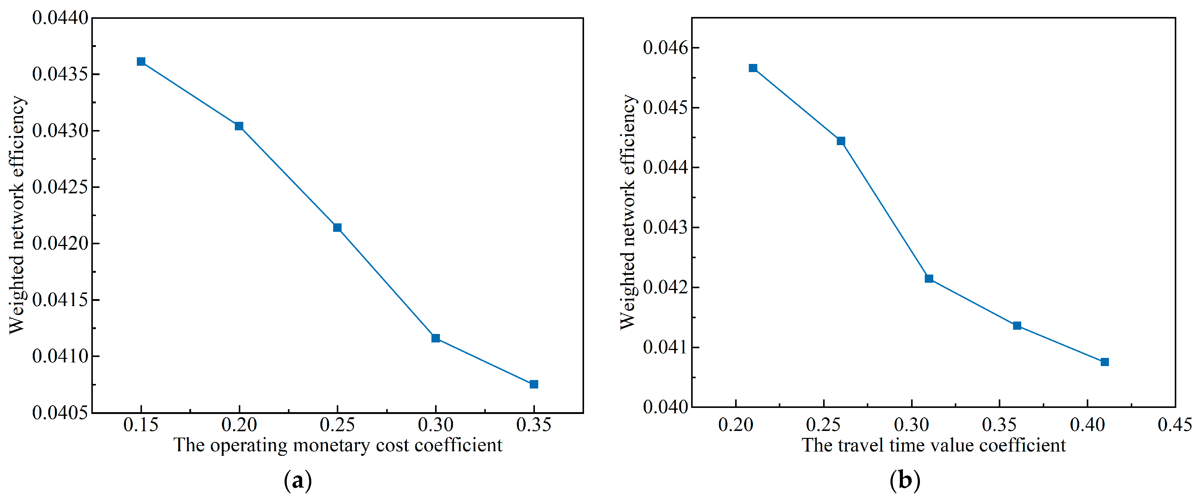
The operating monetary cost coefficient, η 1 = 0.25.
l i The actual length of station section i.
η 2 The travel time value coefficient, η 2 = 0.31.
t i The actual time to pass through station segment i.
η 3 The crowding value coefficient, η 3 = 0.245.
q The average number of passengers in a vehicle.
c The rated passenger capacity of a vehicle.
η 4 The carbon trading value coefficient, η 4 = 0.06.
μ The carbon emissions from the electricity consumed per kilometer.
F j The cost of passing through transfer section j.
c j The number of passengers who need to transfer.
t j The time to walk through transfer section j.
η 5 The walking time value coefficient, η 5 = 0.31.
v i The node number.
C a The node reachability.
f i j The generalized cost of the shortest path from node i to node j.
σ i j Whether node i is connected to node j. If node i is connected to node j, then σ i j = 1; otherwise, σ i j = 0.
C b The path importance.
ε s t The number of shortest paths between node s and node t.
ε s t ( v i ) The number of nodes that the shortest path between node s and node t passes through, v i .
N The total number of nodes.
C d The node degree centrality.
k i The node degree value.
C w The local strength of the node.
w i j The generalized cost between node i and its adjacent nodes.
P i j The information entropy value of the j-th indicator.
W j The weight of the j-th indicator.
C j The amount of information contained in the j-th indicator.
σ j The standard deviation of the j-th indicator.
e j The information entropy of the j-th indicator.
r t j The correlation coefficient between indicator t and j.
B + / B The positive ideal solution and the negative ideal solution.
D i + / D i The Euclidean distance of each node to the positive ideal and the negative ideal solution.
C i The relative progress of each node.
R ( t ) The network resilience at time t.
F ( t ) The network resilience measurement index.
t s The initial time when the network is disturbed.
θ The number of subnetworks.
T i The number of nodes contained in the i-th connected subgraph.
T The number of nodes contained in the largest connected subgraph of the initial network.
E The global reachability.
Table 2. Bus and subway line operation information.
Line NumberTypeDeparture Interval (min)Rated Passenger CapacityAverage Passenger Capacity
0001Bus3.758646
0002Bus7.58654
1001Subway3.831460724
1002Subway4.971460588
Table 3. Information required for weighted network construction.
Previous Station
(Coordinates)
Next Station
(Coordinates)
Distance
(m)
Time
(min)
Comfort CostEnvironmental Cost Generalized Cost
Grand Skylight Community
(126.694505, 45.697257)
Linji Community
(126.68852, 45.702617)
7522.590.1090.0361.090
Linji Community
(126.68852, 45.702617)
Haci Group
(126.684628, 45.705962)
4792.080.1090.0230.944
Harbin West Railway Station
(126.5792, 45.706279)
Chengrong Road
(126.567547, 45.712029)
112020.0820.0991.084
Chengrong Road
(126.567547, 45.712029)
Gongnong Street
(126.558642, 45.718798)
100420.0820.0891.044
Table 4. Analysis of transportation network characteristics in Harbin.
Network IndicatorsBus NetworkBus–Subway NetworkBus–Subway Network Changes Compared to Bus Network
Number of nodes182718923.56%
Number of edges2860320111.92%
Maximum connected subgraph182718923.56%
Weighted network
efficiency
0.040000.042145.26%
Table 5. The top-20 nodes sequence of the weighted network under different evaluation indicators.
IndicatorTop-20 Nodes Sequence
Weighted coreness37, 1841, 77, 1538, 40, 625, 39, 114, 244, 1842, 38, 1859, 282, 1877, 355, 486, 571, 1834, 1119, 611
Path importance46, 226, 37, 391, 1877, 40, 74, 185, 327, 1859, 86, 192, 244, 353, 383, 752, 1842, 7, 84, 96
Reachability38, 1839, 47, 133, 1180, 37, 1840, 1842, 39, 1841, 1838, 40, 41, 1642, 1843, 77, 365, 48, 78, 239
Critical node37, 40, 1842, 244, 77, 1841, 38, 1859, 1877, 41, 114, 39, 48, 383, 46, 981, 85, 188, 752, 316
Table 6. Comparison of network resilience values for different attack and recovery sequences.
Network IndicatorNetwork Connectivity CoefficientGlobal Accessibility
Sequence Attack ProcessRecovery ProcessResilienceAttack ProcessRecovery ProcessResilience
Critical nodes0.122820.772310.4475650.073300.701950.387625
Reachability0.293690.567160.4304250.176690.497710.337200
Path importance0.190560.710960.4507600.106730.69320.399965
Weighted coreness0.220330.672780.4465550.138020.563050.350535
Random0.254970.633260.4441160.177590.535370.356480
Table 7. Comparison of resilience values between bus–subway composite network and bus network.
Network IndicatorNetwork Connectivity CoefficientGlobal Accessibility
Sequence Bus
Network
Bus–Subway
Network
PercentageBus
Network
Bus–Subway
Network
Percentage
Critical nodes0.43420.44762.99%0.37640.38762.98%
Reachability0.41930.43042.58%0.33330.33721.17%
Path importance0.43490.45083.53%0.38790.40003.12%
Weighted
coreness
0.43450.44662.71%0.34710.35050.98%
Random0.42730.44413.78%0.342980.35653.94%
Disclaimer/Publisher’s Note: The statements, opinions and data contained in all publications are solely those of the individual author(s) and contributor(s) and not of MDPI and/or the editor(s). MDPI and/or the editor(s) disclaim responsibility for any injury to people or property resulting from any ideas, methods, instructions or products referred to in the content.

