Abstract
Accurate measurement of track irregularity and the corresponding spectrum is essential for evaluating the performance of transportation systems. Chord measuring methods can achieve fine accuracy but are limited by waveform distortion and a restricted range of recoverable wavelength. To address this, this work explores the effectiveness of integrating inclination data in chord-based measurement to obtain a higher precision and more reliable spectrum. Firstly, the theoretical principles and mathematics of the proposed method are described. We demonstrate that by utilizing inclinometer sensors, the measuring reference can be maintained throughout the measurement, therefore obtaining an authentic waveform of track irregularity. Adaptive technics are employed to examine and extract cumulative components in the measured signal, which also benefits the accuracy of spectral estimation. Error analysis is then conducted by simulated sampling. Furthermore, a case study of field measurement and numerical simulation via multi-body dynamics for a monorail system is presented. The results verify the accuracy and robustness of the proposed method, showing that it provides a broader range of recoverable wavelength, minimum parametric interference, and advantages of signal authenticity. The simulation results prove the significant effects of track irregularity on the dynamic response of the monorail system, hence revealing the value of the presented methods and results.
Keywords:
track irregularity; measurement; inclination; chord reference methods; trend extraction; monorail transit systems MSC:
60G35; 62-07; 62P30; 74H99
1. Introduction
Track irregularity refers to the surface irregularity in general supporting structures in transportation systems including highway [1], railway [2,3], and monorail systems [4,5]. Current studies have shown that track irregularity is the main excitation of effects of the vehicle–bridge interaction [6,7]. This is because the presence of track irregularity will directly change the contact relationship between the vehicle and the track, which in turn affects the position of the bogie and the car body, and ultimately affects the dynamic response of the transportation system including the running safety and riding comfort. Hence, an accurate measurement of track irregularity in the time or spatial domain is essential for the evaluation of track irregularity and its potential effects on transportation systems. In engineering applications, spectral estimation is employed to obtain the power spectral density (PSD) versus wavelength curve (known as the spectrum) of track irregularity so that its non-stationary features in the frequency domain can be characterized. Such approaches allow us to propose a general spectrum fitted by various mathematical forms. For instance, many regions including the U.S., Germany, and China have developed their own standard spectra of track irregularity for railway systems based on detailed measurements. These spectra generally contain multi-level curves to meet different conditions of the track line. In addition, the spectral characteristics of different transportation systems typically differ because of diverse structural configurations. Therefore, the choice of spectrum curve in research generally depends on the problem to be solved and the true states of the track line.
In general, two main principles have been applied to measure track irregularity, i.e., the inertial reference method (IRM) and the chord measuring method (CMM, also known as the chord reference method). IRM-based methods construct a relatively static reference by making use of the fact that the vibration frequency of vehicular parts is much higher than the natural frequency of the detecting system. Then, track irregularity is measured by accelerometers, global navigation satellite systems, etc., as described in [8]. CMM-based systems [9,10] take a completely different approach—they construct the reference by connecting the measuring points fixed at both ends of the testing systems and then measure the relative distance between the reference and track surface.
Significant works have been reported on the design or application of measuring processes in railway systems based on IRM or CMM. Peng et al. [11] designed a comprehensive detection system for rail track geometry by fusing visual and inertial sensors. An accelerometer and a Kalman filter were used to eliminate accumulated unrealistic drifts of the accelerometer and gyroscope. Lee et al. [12] described a method of estimating irregularities in railways using acceleration data measured from high-speed trains. Sun et al. [13] developed an algorithm via IRM and multiple digital filters to derive longitudinal level irregularity from the acceleration measured in the axle box of a high-speed train. Similarly, the application of inertial sensors (e.g., accelerometers) mounted on an in-service train and Kalman-based filter (e.g., the extended Kalman particle filter) can be found in the works by Muñoz et al. [14] and Lathe et al. [15]. Relevant works have also been performed in other rail transportation such as maglev systems [16]. It should be noted that inspections of track geometry can be also divided into static and dynamic phases depending on whether dynamic axle loads are used. Static inspection of track geometry reflects the long-term accumulation of residual track deformation. IRM systems are generally integrated into dynamic inspection to capture the track irregularity under loading conditions, while CMM systems are applicable in both scenarios. In addition, IRM systems are more easily affected by vibration factors such as the testing speed [17], and the realization of IRM systems is more complicated and costlier compared with CMM systems.
However, there are certain limitations in the use of CMM, including the distortion of measured waveform and restricted ranges of recoverable wavelength (i.e., frequency range in the spectrum). This is because the measuring baseline of CMM varies with the change in random measuring position and cannot reflect the actual track irregularity. Despite their transfer functions being definable, the values of these functions inevitably fluctuate across the entire frequency domain. Consequently, complementary functions for signal reconstruction are naturally volatile within the frequency domain as well. Therefore, the recoverable range is restricted to avoid the occurrence of high errors in reconstruction. Restoration methods including multipoint chord reference systems [18,19] were developed to address these issues and achieve fine results in numerical analysis.
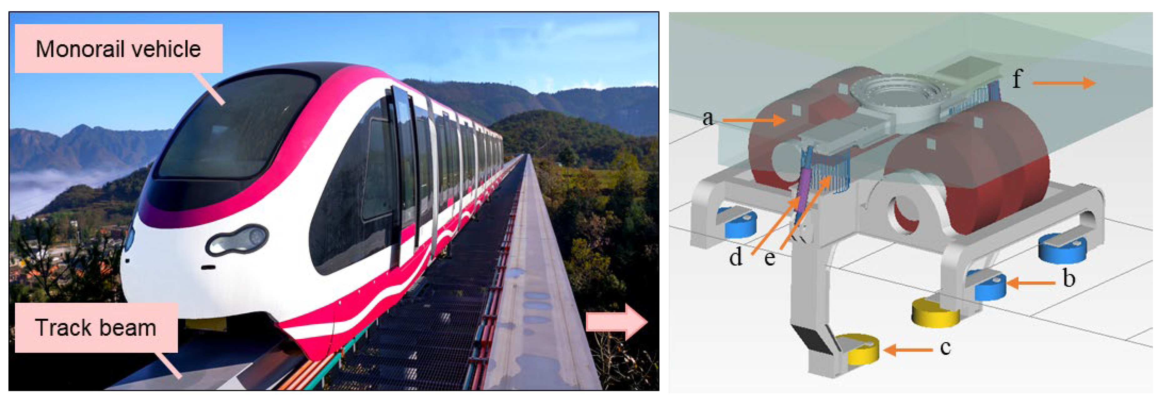
It should be noted that the existing research on track irregularity predominantly concentrates on railway systems, and there are very few studies and datasets available regarding monorail systems. Monorail systems have been widely used in urban and tourist transportation because of their superior security, strong line adaptability, and environmental friendliness [20]. In monorail tour transit systems (MTTSs), a monorail vehicle constantly encircles and runs along a steel single-track beam during vehicle operations (see Figure 1). The use of a steel beam satisfies the requirements of efficient prefabrication and installation. However, it also results in a more flexible structure with a relatively higher live load, thereby causing problems in the control of track irregularities. A previous study presented the measured spectrum of track irregularity in various MTTS projects but still lacks details for signal processing and corresponding error analysis [21]. It is also worth noting that the existing research predominantly utilizes an irregularity spectrum derived from a 34.8 m long track beam [22]. For instance, Gou et al. [23] adopted it and studied the dynamic response of a long-span arch bridge under monorail and truck loadings by combining numerical analysis and field tests. Kim et al. [24] used it and investigated the effect of monorail trains on the seismic responses of a monorail bridge under ground motion. Nevertheless, owing to the random and nonstationary features of track irregularity [25], the sample size of Japanese data is far from sufficient. Generally, the calculation length of track irregularity should be greater than five times its maximum wavelength (generally, 30–100 m). Additionally, although extensive data on track irregularity are available for railway and highway systems, directly applying those spectra to a monorail system is not suitable because of the significant differences in track configuration. Simply put, there is limited information available on the track irregularity in monorail systems.
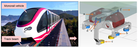
Figure 1.
Overview of an MTTS project located in Liupanshui, China, and the typical configuration of the bogie of a monorail vehicle: (a) traveling wheels; (b) steering wheels; (c) stabilizing wheels; (d) hydraulic shock absorber; (e) air suspension; and (f) car body.
In this work, we further examine the effectiveness of using inclination data in chord methods to form a measured dataset. Moreover, simulations and field tests are presented to provide evidence of applicability. To promote the use of CMM-based methods in general transportation systems, the presented case study was carried out in a practical MTTS project. The rest of this work is structured as follows. Section 2 gives a comprehensive description of methodologies for measuring and signal processing. Moreover, relationships between CMM and the proposed method are revealed. Section 3 presents the data analysis and results of simulation sampling and a case study based on the field test and numerical simulation for an MTTS project. Finally, the conclusions are drawn in Section 4.
2. Methodologies
2.1. Measuring Method
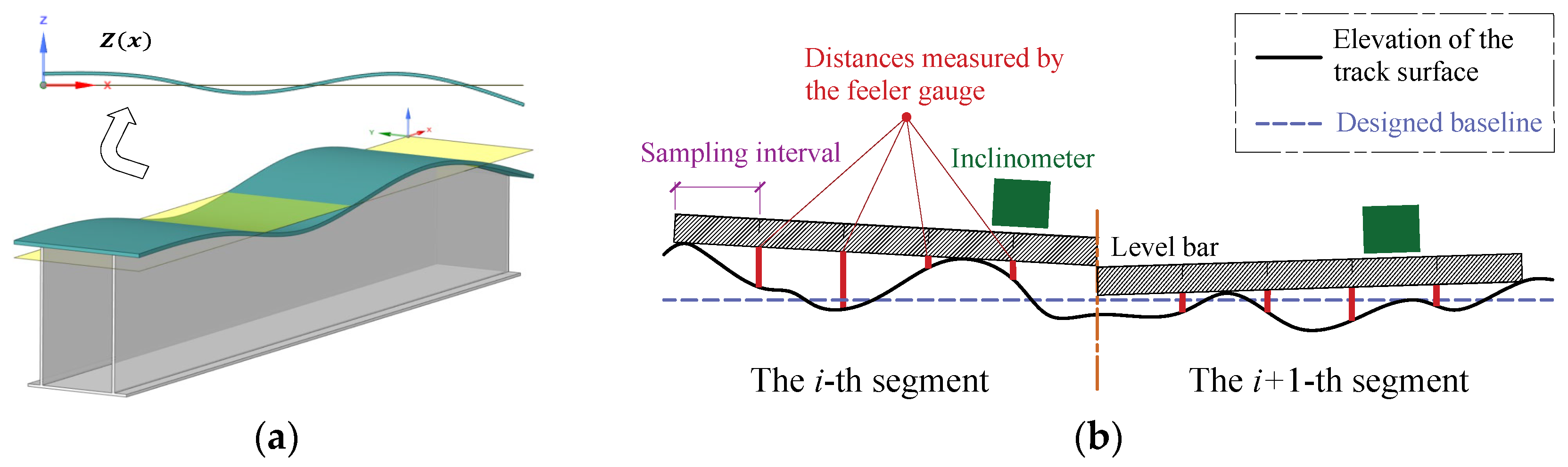
As previously discussed, implementing IRM-based systems is time-consuming and expensive, whereas CMM-based systems have their own set of limitations. To address this, we propose measuring the true waveform of track irregularities by incorporating an inclinometer into the conventional measuring process, referred to as the inclination correction method (ICM). It should be noted that the measured dataset for ICM can be obtained either automatically (e.g., using laser displacement transducers, digital theodolites) or manually. For easy demonstration, this work presents a manual method for measuring the longitudinal track irregularity (LLI) of monorail systems, as shown in Figure 2. Here, the LLI refers to the deviation between the actual and designed position of the top plate of the track beam.
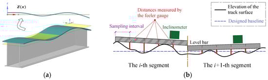
Figure 2.
(a) Definition of the LLI for the track beam in monorails. (b) Configuration of equipment and measuring process of ICM. In each segment, the inclination of the level bar and the gap between the bar and track surface are measured, respectively.
The basic equipment used by ICM is the level bar, high-precision inclinometer, and feeler gauge. Field measurement is conducted in segments. To ensure continuity in the measured data, the starting point of each segment is set to the terminal point of the previous segment. Note that the feeler gauge measures the average value of the track irregularity on the track cross-section, which is especially suitable for monorail beams since the rubber tires of monorail vehicles have a certain thickness. The processes of ICM in each segment are illustrated in Figure 3 and described as follows.
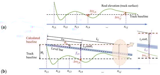
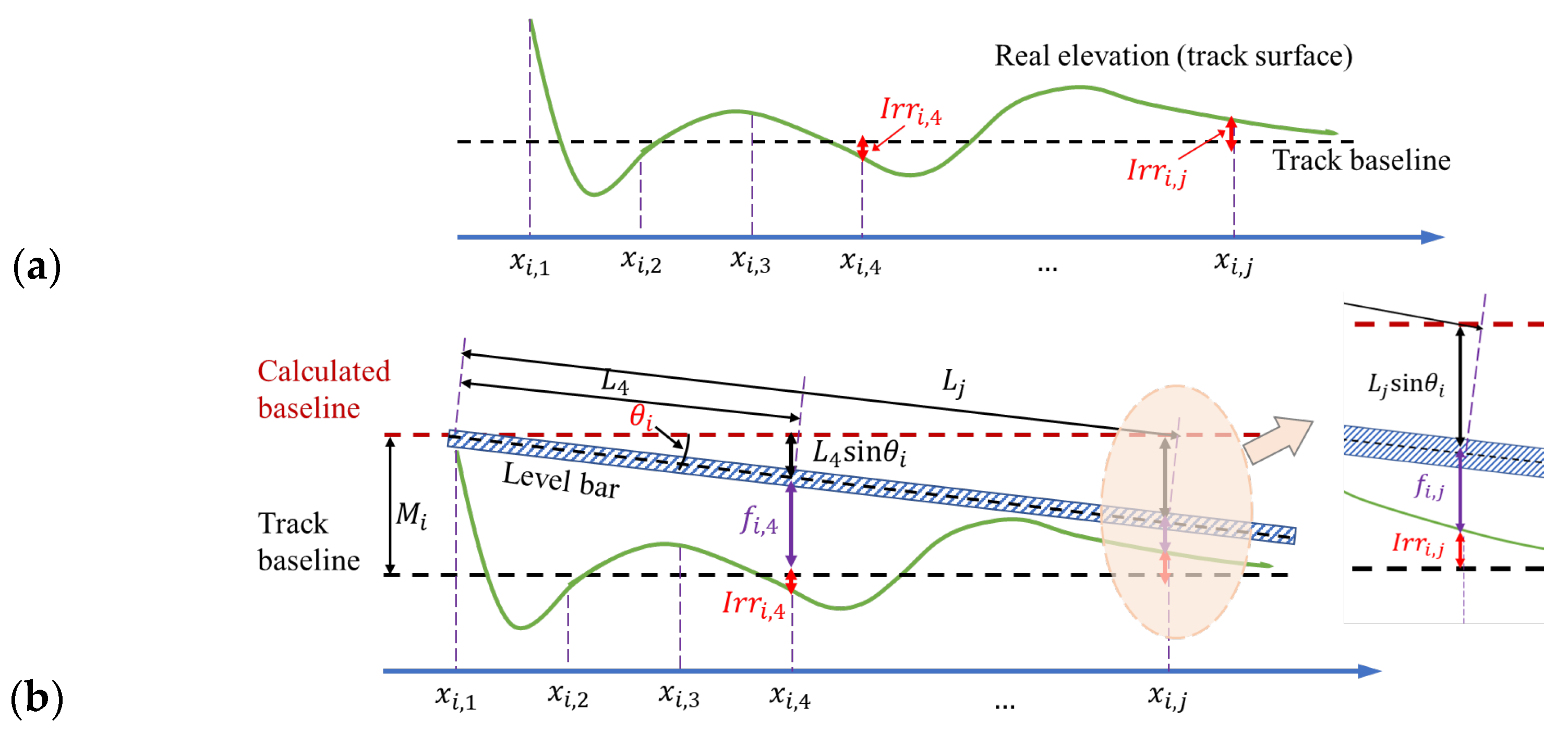
Figure 3.
Measuring principle of ICM: (a) definition of track irregularity and (b) mathematical relationship in the measurement of each segment.
- (i)
- Take the -th segment as an example. As Figure 3a shows, the green line indicates the uneven surface of the track beam. Then, the track irregularity at point is the distance between the green curve and the real baseline (unknown), denoted by .
- (ii)
- The inclination of the level bar is obtained by the inclinometer, while the gaps between the level bar and the track surface are measured by the feeler gauge, as shown in Figure 3b. With the inclination and the known total length of the level bar (), the distance between the calculated baseline and the track baseline () is constant and, hence, we have Equation (1):where denotes the -th point in the segment and is the measurable data, given by . Based on sign rules, is positive when the surface elevation is over the baseline; otherwise, it is negative (e.g., in Figure 3). is positive when the calculated baseline is obtained by rotating the ruler counterclockwise (e.g., in Figure 3); otherwise, it is negative.
- (iii)
- Equation (1) relates the track irregularity of the first point to the others in each segment. For the end point in the segment , we have using Equation (1). Since the true value of track irregularity at each point depends only on the track condition, we have . Repeatedly, using Equation (1), the values in segment can be determined by . Then, the entire data can be obtained by using Equation (2).where means the end point.
Thus far, we can obtain the values of track irregularity by determining —the value of the global starting point. In fact, the value of does not affect the relative magnitude of any other points but the overall translation of the distribution curve. Two methods can be used to determine this value. First, a leveling elevation survey can be conducted. Second, studies have proven that track irregularity can be regarded as a stationary random signal approximately in engineering applications. That is, the value of can be assigned based on the statistical characteristics of the overall measured data. For example, it can be set to satisfy the condition that the mean value of the entire dataset is zero.
For track lines with a specific alignment (e.g., slope), the track baseline is no longer straight but follows the variation in it, resulting in a long-term trend () in the measured data. A detailed trend extraction method is present in Section 2.3, but it is recommended to remove this term in advance simply using if the original design blueprint is available.
2.2. Relationship between ICM and CMMs
According to the parametric settings, such as the total number and intervals of measuring points, CMMs can be divided into various categories such as the three-point equal method, three-point offset method (TPOM), four-point offset method (FPOM), etc. Taking the TPOM as an example, let us review its principle shown in Figure 4 first. As shown, the reference of TPOM is established by connecting the measuring points at both ends of the equipment; the chord value is measured with the use of CMM.
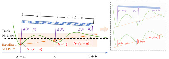
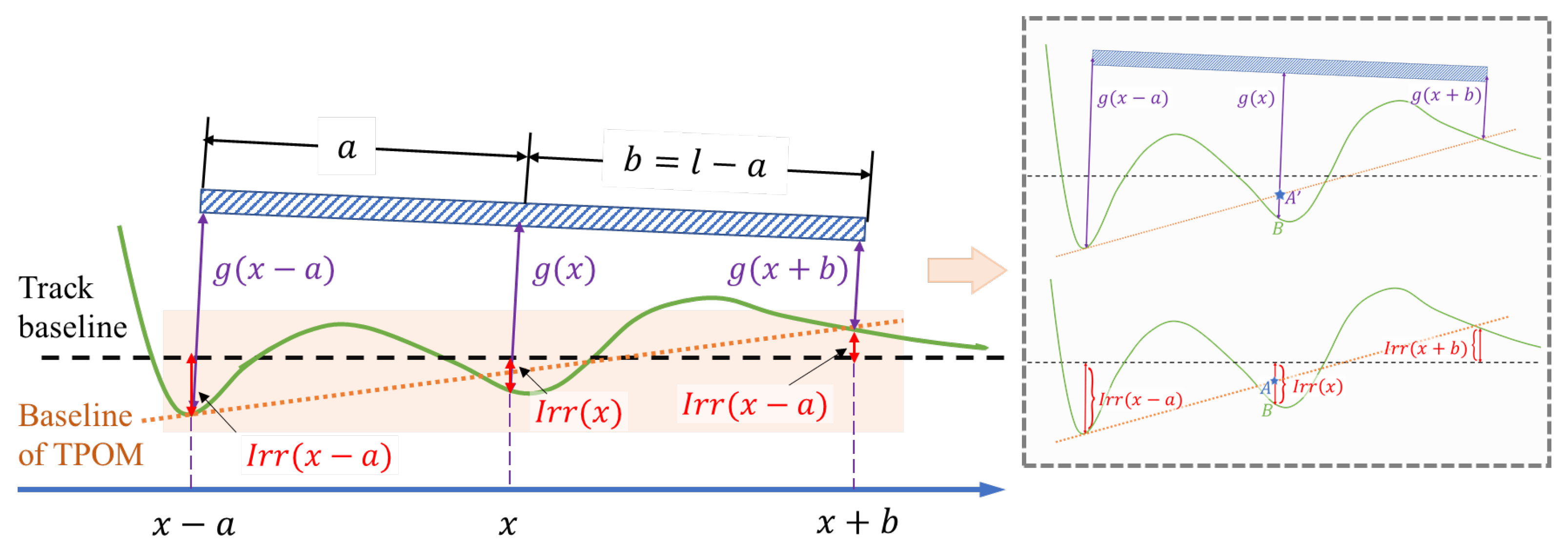
Figure 4.
Testing principle of TPOM. Note, the green line is the real elevation of track surface, is the actual value of track irregularity, while is the measured value, and their relationship is shown in Equations (3) and (4).
Then, since the chord length () is much greater than the value of track irregularity, we use to depict the relationship between the measured value and the track irregularity , as defined in Equation (3). Obviously, the reference of TPOM is variable at different position of the track surface with the movement of the measuring instrument.
where m(x) is the measured chord value using CMM and a, b, and l are parameters of CMM.
By transforming Equation (3) of the space domain into Equation (4) of the frequency domain, we can discover this effect more clearly. That is, the value of is precise when that of equals 1, which can never be assured under the whole frequency range. In fact, the magnitude of varies from 0 to 2 with the change in frequency (i.e., the wavelength from another perspective)—just like a wave filter. Consequently, the data measured by TPOM are not the actual value of the track irregularity, nor are other CMMs with different parameters.
where is the so-called transfer function, refers to the spatial frequency, and is the wavelength of the track irregularity.
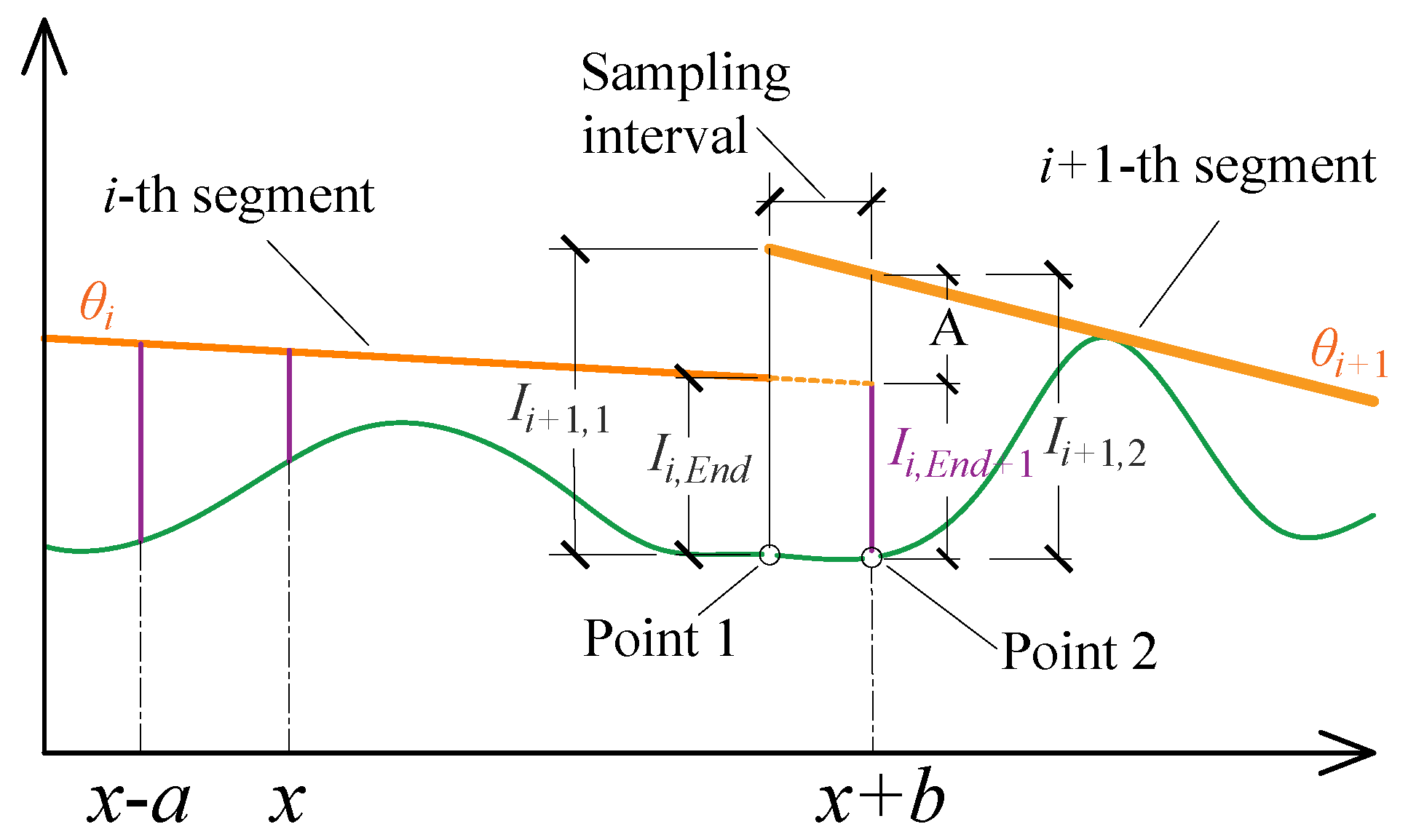
Typically, we can adopt an accordingly designed filter whose magnitude response is reciprocal to that of to address this effect. Specific examples will be given in the simulation and case study later. By comparing the principle of ICM with CMM, we can easily discover their relationship. Specifically, ICM measures the track irregularity under a steady reference in each segment, and the differences between different segments can be modified by the measurement of inclination. As for CMM, it measures the amplitude of midpoint(s) relative to the endpoints; therefore, the calculated result by using Equation (3) is constant if the references are all straight. On these bases, data obtained by ICM can be analyzed via the CMM process. For example, assuming that the parametric settings of the TPOM are , , and , with the sampling interval of in ICM, we have and . In addition, when the group data span two testing segments—in this case, when —we adopt Equation (5) to ensure the data are obtained under the same reference of ICM, as shown in Figure 5.
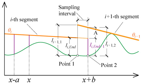
Figure 5.
Extrapolation at the ending point of segment using data from segments and Note, the orange and green lines are the level bar and track surface, respectively.
2.3. Trend Extraction Method
Track irregularity is generally expressed by the function of its PSD to express its characteristics and allow application in subsequent studies. Nevertheless, owing to manual calibration, temperature drift of the sensors, or data transmission, the measured data of track irregularity usually contain global trend components [17]. Similarly, while using ICM, the process of obtaining the cumulative sum of the correctional value (i.e., in Equation (2)) may result in a low-frequency and high-amplitude trend, thereby bringing high error in subsequent spectral analysis. Moreover, the composition and causes of the trend components are too complex to identify immediately. Therefore, research on the trend extraction of measured track irregularity is necessary. In addition, the application of trend extraction will serve to eliminate the error caused by the alignment settings (i.e., mentioned in Section 2.2) of the track beam.
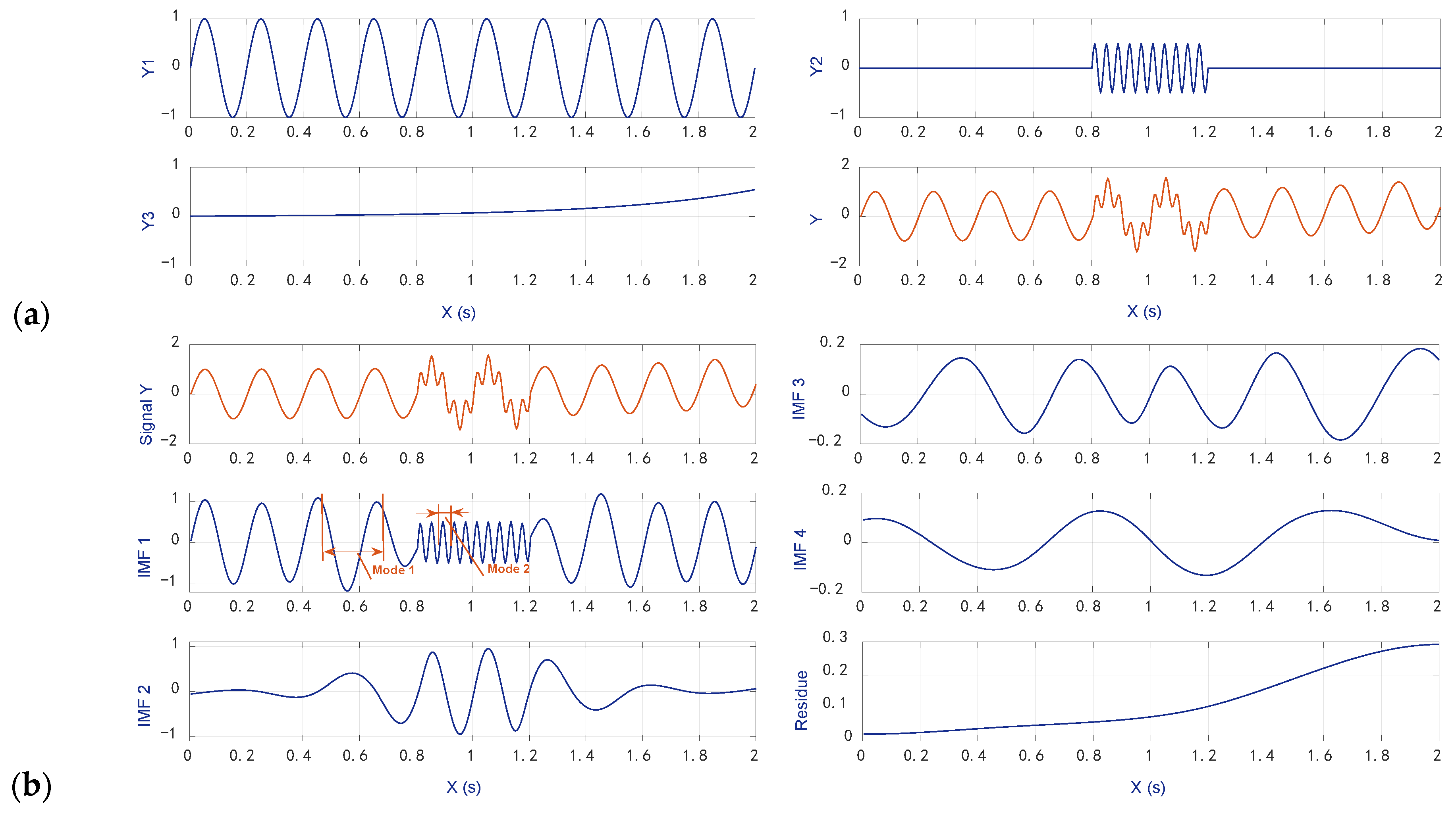
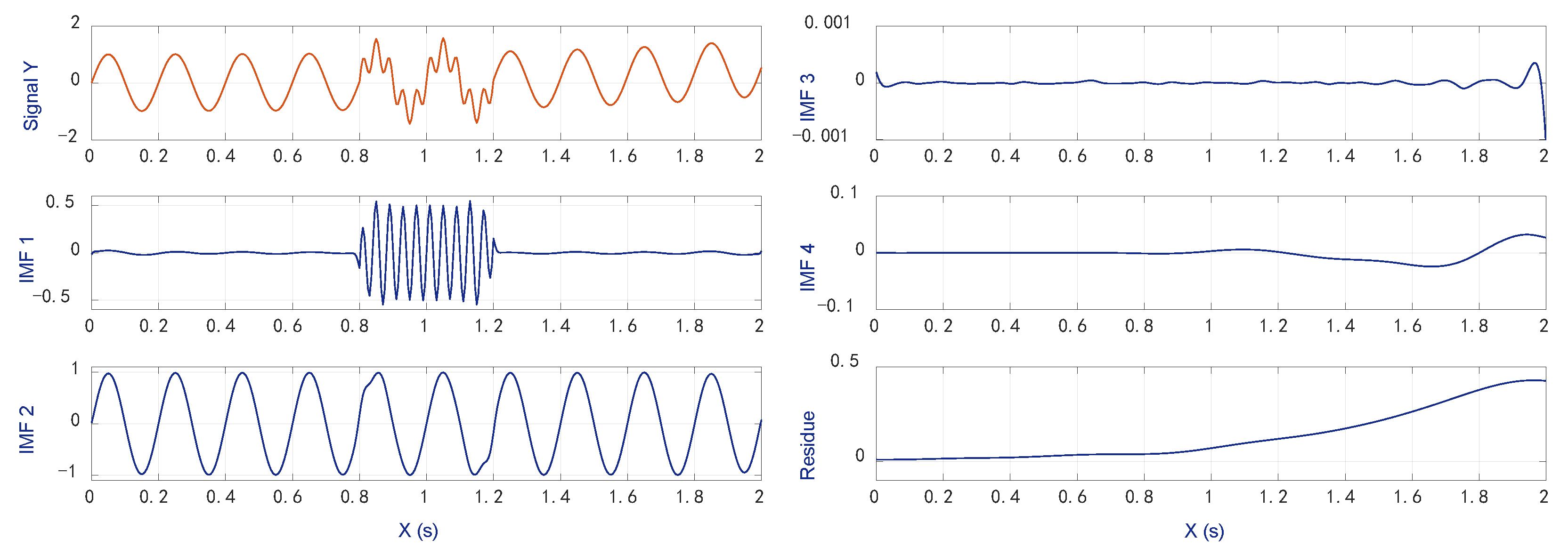
The process of trend extraction mainly includes two phases, i.e., decomposing the original signal into several components and then determining the trend components among them. In order to minimize the error caused by data analysis, the extraction process should be as adaptive as possible. For example, the well-known empirical mode decomposition (EMD) [26] can be adopted since it decomposes the signal totally based on its own characteristics. It should be noted that according to the principle of EMD, intrinsic mode functions (IMFs) of high frequency will be obtained first. Since the trend is a slowly varying and long-term component, it is intuitive to construct it by summing the low-frequency modes (i.e., the posterior IMFs) and the residue. Significant works have been reported on this issue, and three of them [27,28,29] are illustrated in Figure 6. To examine the applicability of different identification methods, let us first examine an artificial signal consisting of two trigonometric functions () of distinct dominant frequencies plus a long-term trend component (). Then, we decompose the artificial signal by EMD, as shown in Figure 7.
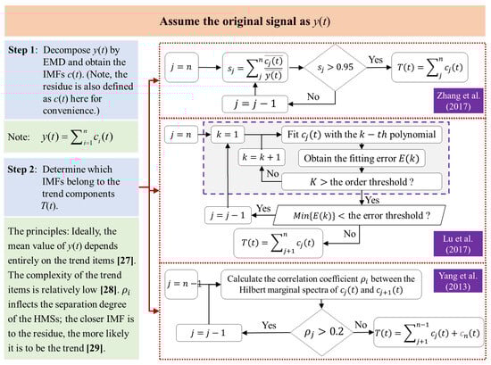
Figure 6.
Process of different EMD-based methods for trend identification: decompose the original signal first and then determine the trend components based on signal characteristics. Three methods presented by Zhang et al. [27], Lu et al. [28], and Yang et al. [29], respectively, are summarized. Note, HMS refers to the Hilbert marginal spectrum of each IMF.
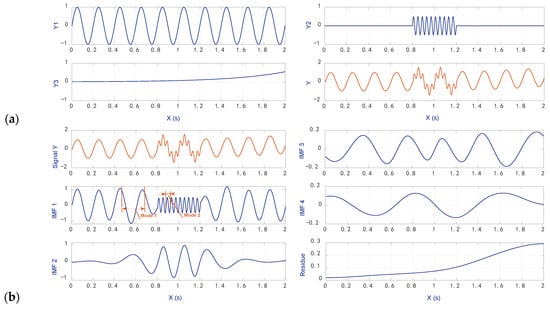
Figure 7.
Decomposition result of an artificial signal using EMD. (a) Signal and its components: , , , and ; the analog sampling frequency is 200 Hz. (b) IMFs 1 to 4 and the residue decomposed by EMD.
Figure 7b indicates that the decomposed residue is not exactly the long-term components we predefined, nor is any IMF is consistent with the predefine trigonometric functions. The main reason for this is the existence of mode mixing, which is one of the principal deficiencies of EMD. Mode mixing is defined as a single IMF either comprising signals of widely disparate scales or a signal of a similar scale residing in different IMFs [26]. In Figure 7, mode mixing occurs in the first IMF, thereby affecting the following IMFs and the residue. Since mode mixing directly affected the characteristics of all these components, the identification process is influenced consequently.
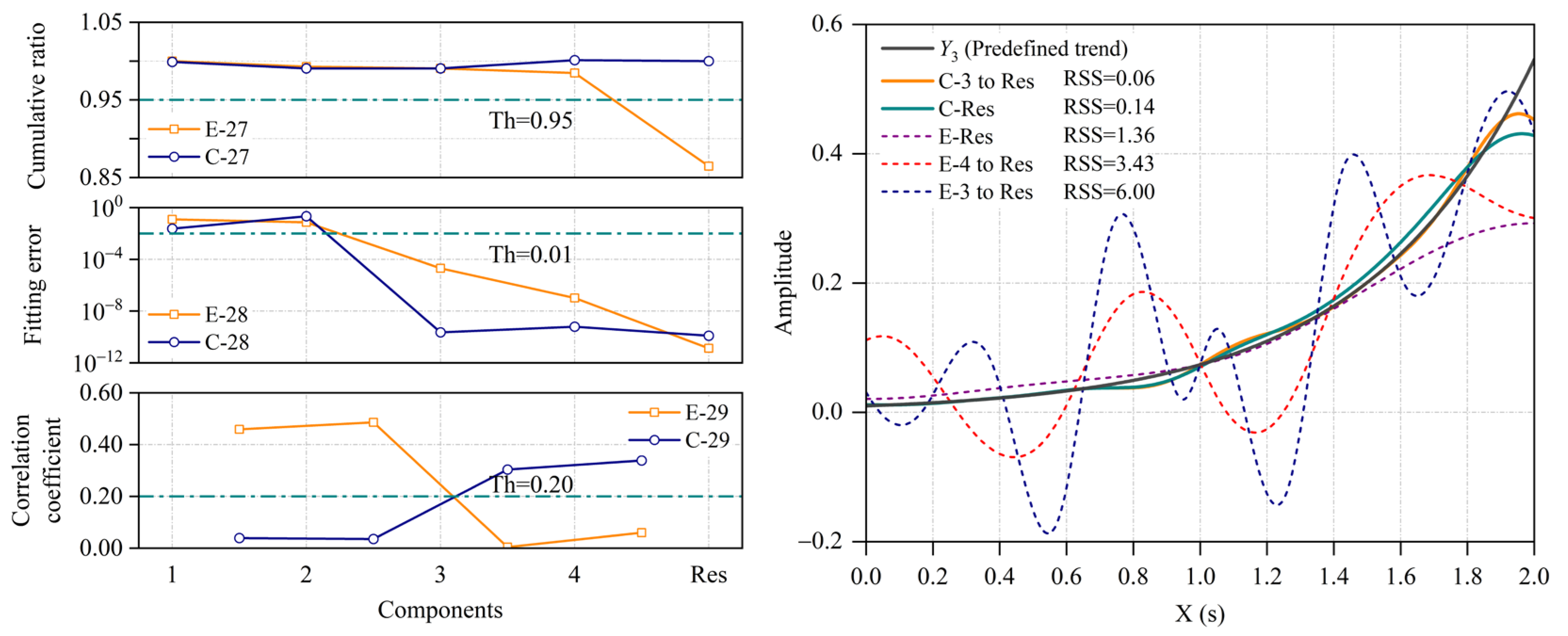
To solve this, we recommend decomposing the signal by an improved EMD—complete ensemble empirical mode decomposition with adaptive noise (CEEMDAN) [30]. CEEMDAN solves mode mixing by performing EMD over an ensemble of the signal plus selected white Gaussian noise and populating the whole time–frequency space; moreover, the residue at each mode is uniquely computed. The specific process can be found in [30]. For comparison, the decomposition result of signal using CEEMDAN is shown in Figure 8. A comparison of Figure 7 and Figure 8 clearly shows that the components obtained by CEEMDAN are more consistent with the predefined items. Specifically, IMF 1 and IMF 2 of CEEMDAN agree well with and , respectively, although a small fluctuation in amplitude can be found. Next, we apply the above identification methods and use the residual sum of squares (RSS, see Equation (6)) to quantify the proximity of the obtained trend to . Relevant results are shown in Figure 9.
where is the sample size, are the observed values, and are the estimated values.
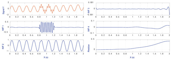
Figure 8.
Decomposition results of Y using CEEMDAN. Although the same number of components as EMD is decomposed, here, IMFs 1 and 2 are much more consistent with the predefined Y1 and Y2.
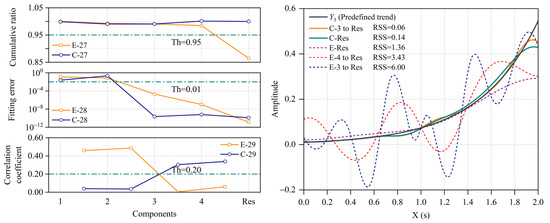
Figure 9.
Results of trend extraction. (left) Identification results by different discriminants in current works; note, ‘E/C-27/28/29’ means the method in [27,28,29] was applied to components decomposed by EMD (E) or CEEMDAN (C), and Th is the threshold value. (right) Comparison of the predefined trend and reconstructed trend items; note, ‘C-3 to Res’ means the trend is the sum of IMF 3, IMF 4, and the residue that was decomposed by CEEMDAN. C-Res and E-4 to Res, E-3 to Res, E-Res, and C-3 to Res are determined by the method in [27], [28], [29], and [28,29], respectively.
Clearly, the identification result is not the same. Specifically, for the components obtained by EMD, the method in [27,28,29] demonstrates that the trend should be the sum of IMF 4 and the residue, IMF 3 to the residue, and the residue alone, respectively. In addition, the residue alone has the smallest value (1.36) of RSS, indicating the method in [29] is more suitable in this case. As for the CEEMDAN-based methods, the method of the ‘cumulative ratio’ indicates that the residue is the only trend item, while others choose the sum of IMF 3 to the residue. The RSS value of identification proves that the latter two methods provide a better solution, especially when the trend amplitude is relatively higher. Nevertheless, no matter what kind of combinations we select, the RSS values of the reconstructed trend using CEEMDAN-based methods are lower than those of EMD-based methods. In summary, the calculation results of signal Y demonstrate the effectiveness and accuracy of the proposed method. For future studies on signal processing (e.g., signal of track irregularity, vibration, time-series datasets, etc.), we recommend decomposing by CEEMDAN to obtain better IMFs and identify them adaptively by calculating the correlation coefficient of the Hilbert marginal spectrum of adjacent IMFs.
3. Simulation and Case Study
In this section, computer simulations will be first introduced to verify the effectiveness of proposed methods; then, a case study will be presented based on the measurement of the LLI of an MTTS project.
3.1. Computer Simulation
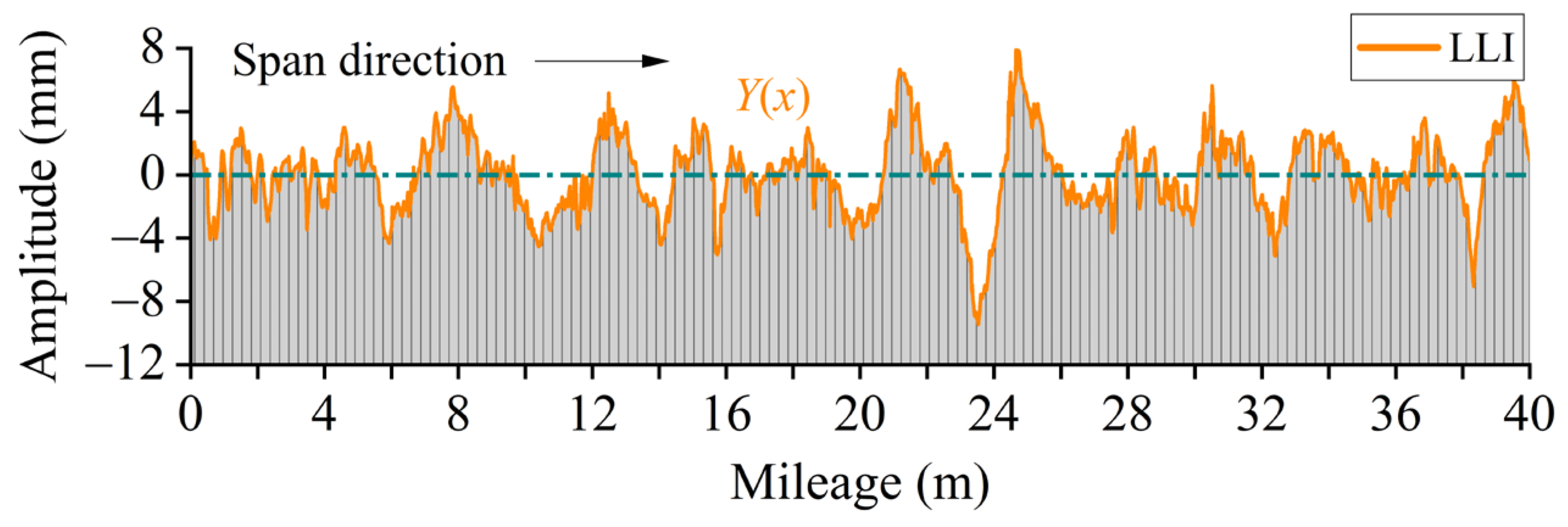
Consider an artificial zone plotted in Figure 10 to represent the track beam. Assuming the baseline is the zero axis, then the upper envelope of this zone, i.e., the orange line Y(x), becomes the elevation of the top plate and, in the meantime, the LLI of the track beam. The simulated sampling frequency and total signal length here are 100 Hz and 40 m, respectively. The measured data are divided into 20 segments, each with a length of 2 m to realize the corresponding processes of ICM.
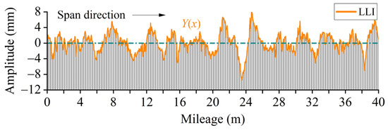
Figure 10.
Overview of the artificial zone and predefined LLI of the track beam.
For the measurement of each segment, the position of the level bar is first determined by the following steps, as illustrated in Figure 11a.
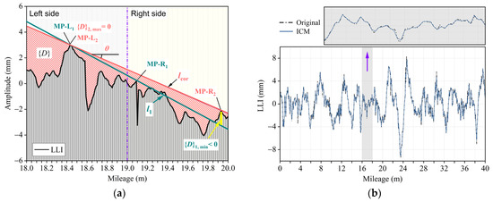
Figure 11.
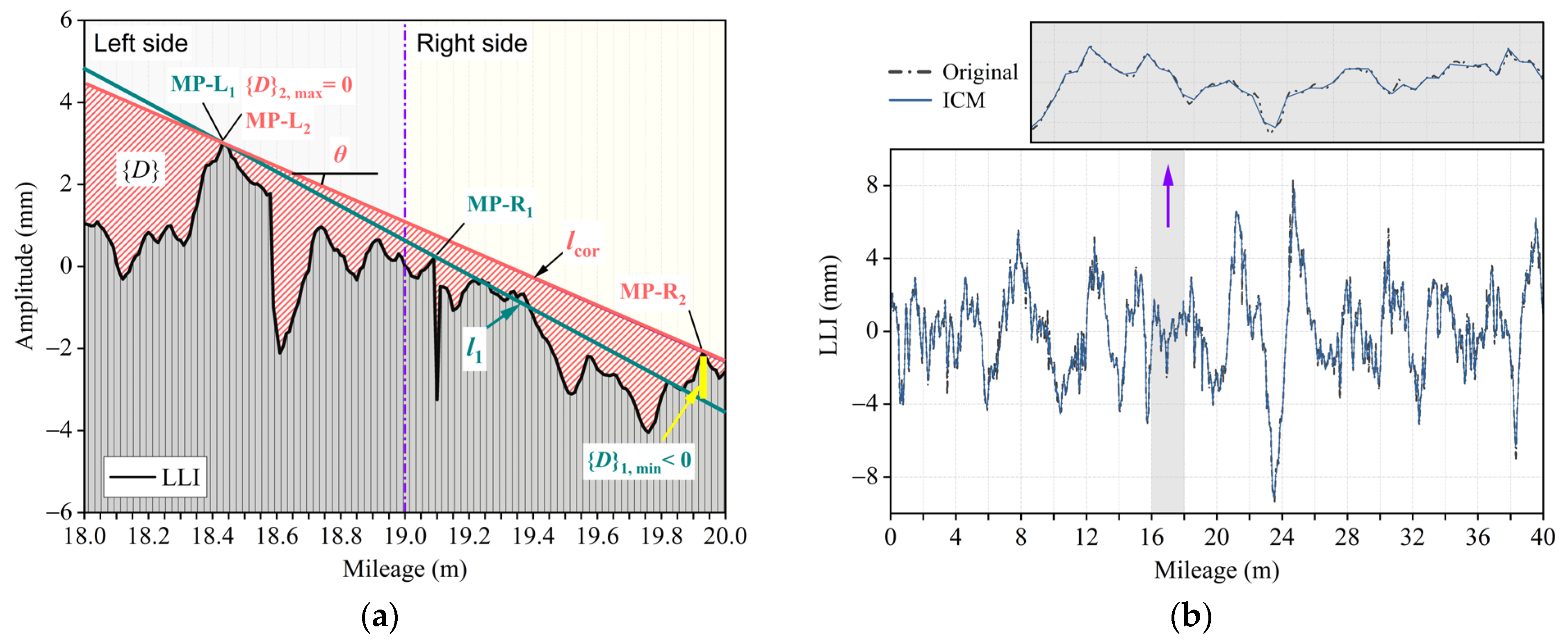
(a) Processes of determining the correct position of the level bar (in the 10-th segment). Afterward, its slope and distance to the track surface (area covered by red slashes) can be measured. (b) Comparison between the distribution curve obtained by ICM and the original data.
Step 1: Discover the maximum point of the curve on each side (denotes max-point-left/right, MP-L/R) and construct a straight line , then obtain the distance between the formed line and the original curve by calculating .
Step 2: If the minimum value of is zero, then is the needed line; if not, find the position of the minimum value, make it the updated point, and build the updated straight line and sequence . Repeat this step until .
Step 3: Finally, obtain the correct position of the simulated level bar (denotes ), where the whole measured value is assured to be non-negative.
Thus far, the sequence measured under is the measured value of ICM in Equations (1) and (2), while the slope of is the measured inclination. With these data, the distribution curves of LLI can be obtained by using ICM, as shown in Figure 11b.
Clearly, the simulated LLI with the actual inclination is entirely coincident with the original data. The only difference between them is due to the discrete sampling process—just as it happens in field tests. Furthermore, observation of Equations (1) and (2) shows that the performance of ICM is mainly affected by the trend caused by the cumulative error of the measured inclination, which we discussed earlier. To examine the robustness of ICM under trend items, we simulate three sequences of as follows: , , and . Here, is the true value, and means a random value between −1 and 1, as shown in Figure 12a. It should be pointed out that the nominal precision of the inclinometer we use in this work is 0.05. That is, the simulated values of 0.15° and 0.25° are three and five times the nominal precision, respectively, which is far greater than the expected error while using ICM. With the same sequence of , the simulated results of the LLI are obtained by the same process of ICM, as shown in Figure 12b.

Figure 12.
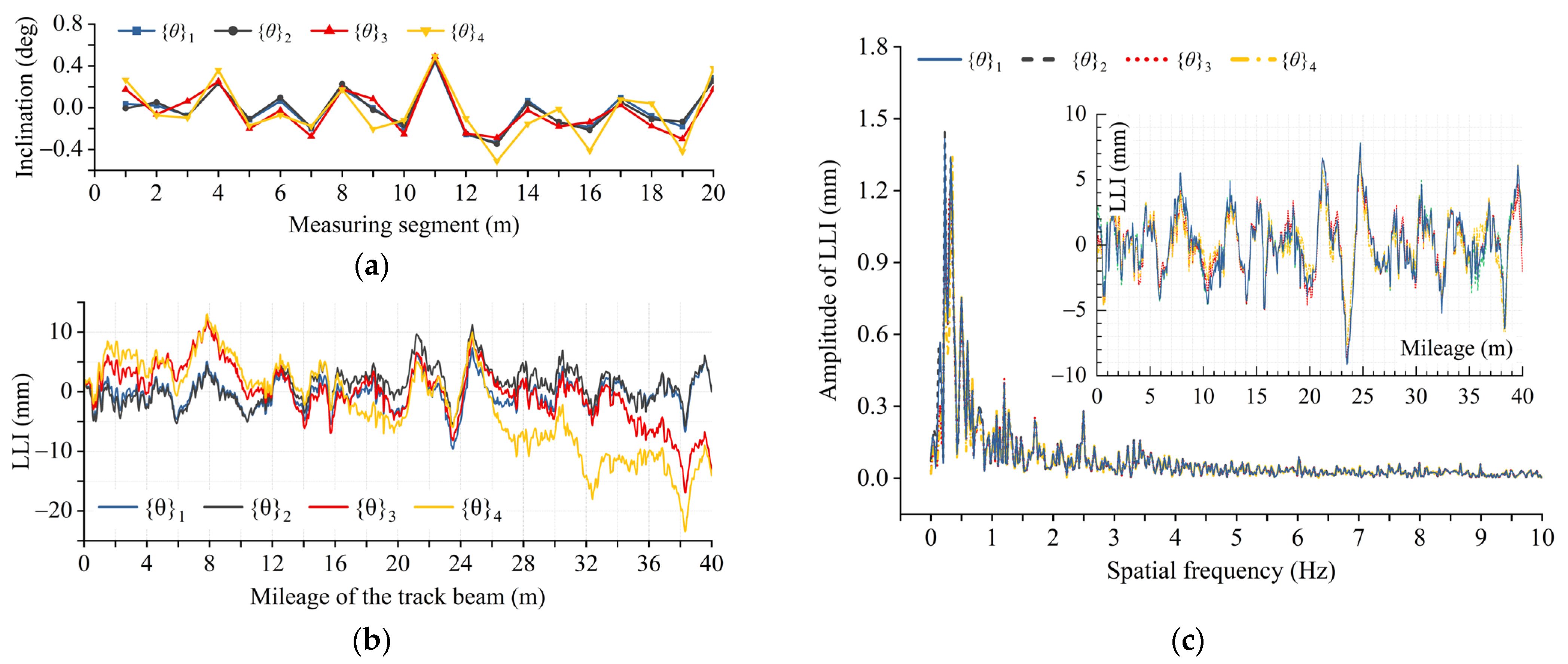
Results of LLI obtained by ICM under different level error of inclination. (a) Distribution of inclination sequences. (b) Obtained curves via various inclination data. (c) LLI after trend extraction and its spectrum.
The simulated results illustrate that under the nominal error, the distribution curve obtained by ICM is consistent with the true value. When the error level grows unpredictably—in this case, three and five times the nominal error—we cannot simply ignore their influence. Nevertheless, the inclination error can only affect the global trend in LLI, not its inherent variation in amplitude. In other words, only periodic, linear translation occurred in the original data. Therefore, after eliminating the trend components via the proposed method, the effect of inclination error can be adaptively offset to a significant extent. Afterward, the overall characteristics of the distribution curves obtained by ICM in the space and frequency domains are highly consistent, as shown in Figure 12c.
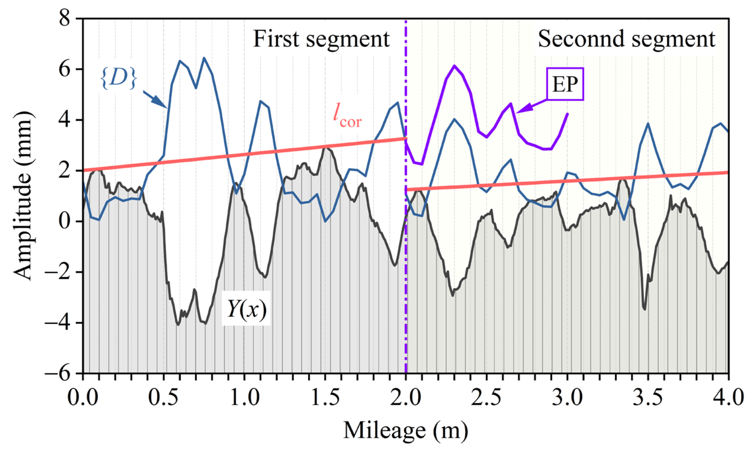
In addition, we also examine the principle shown in Figure 5 by comparing the CMM results extrapolated from the measured data of ICM with those directly obtained using TPOM in a computer simulation, as shown in Figure 13. The process of data extrapolation is essentially translating the data from the next segment, which is also measured under a straight reference . As we discussed earlier, by using Equation (3) or Equation (4), any difference between two good references can be offset, which means the data measured by ICM can be analyzed using a CMM approach after data extrapolation. As we discussed earlier, the value measured by CMM is not true, and a special inverse filter [31] whose magnitude response is reciprocal to that of the transfer function within the recoverable range—empirically, when H(ω) > 0.1—can be adopted to restore the signal. Here, we select TPOM with parameters and . Its recoverable range is 208 to 5535 mm (i.e., 0.18 to 4.81 Hz). Three finite impulse response (FIR) filters with an order of 200, 400, and 800, respectively, are adopted to restore the data.
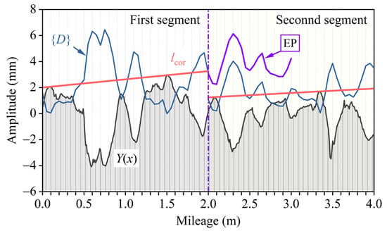
Figure 13.
Diagram of data extrapolation (EP means extrapolation).
Figure 14a shows the magnitude response of filters and that of the H(ω) of the selected TPOM, as well as the restored signal of LLI and the result obtained by ICM. It is demonstrated that the magnitude of the designed FIR filter is reciprocal to that of the transfer function of TPOM. After filtering, the distribution curves of LLI are well restored, as shown in Figure 14b. Note that the signal length will decrease during filtering, which can be offset by simply extending the raw data length.
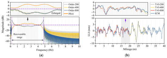
Figure 14.
Comparison of the results obtained by ICM and TPOM; note, T-O-200/400/800 means filters with an order of 200, 400, and 800. (a) Distribution of inclination sequences. (b) Results obtained by ICM and TPOM with various filters.
Compared with the results obtained by ICM, however, TPOM, or any other CMM, can never obtain the actual waveform of track irregularity since some components outside the recoverable range are ignored. In addition, although the increase in filter order improved the magnitude response resolution of FIR filters, they still failed to enhance the performance of data restoration in this case. Furthermore, let us examine the results obtained by ICM and TPOM from a quantitative view via the root-mean-square (RMS) value of the sequences defined as the simulated value minus the true value. In this case, the results of and are 3.58 × 10⁻⁴, 0.31, 0.59, 0.86, 1.25, 1.26, and 1.31 mm, respectively, indicating the performance of ICM is much better. Not to mention the simulated error of ICM here has far exceeded expectations.
In summary, the simulation results above strongly verify the proposed methods. A comparison of results indicates the advantages of ICM in measuring accuracy and waveform authenticity of track irregularity since it is not limited by the wavelength range or the specific selection of parameters or function types.
3.2. Measurement in an MTTS Project
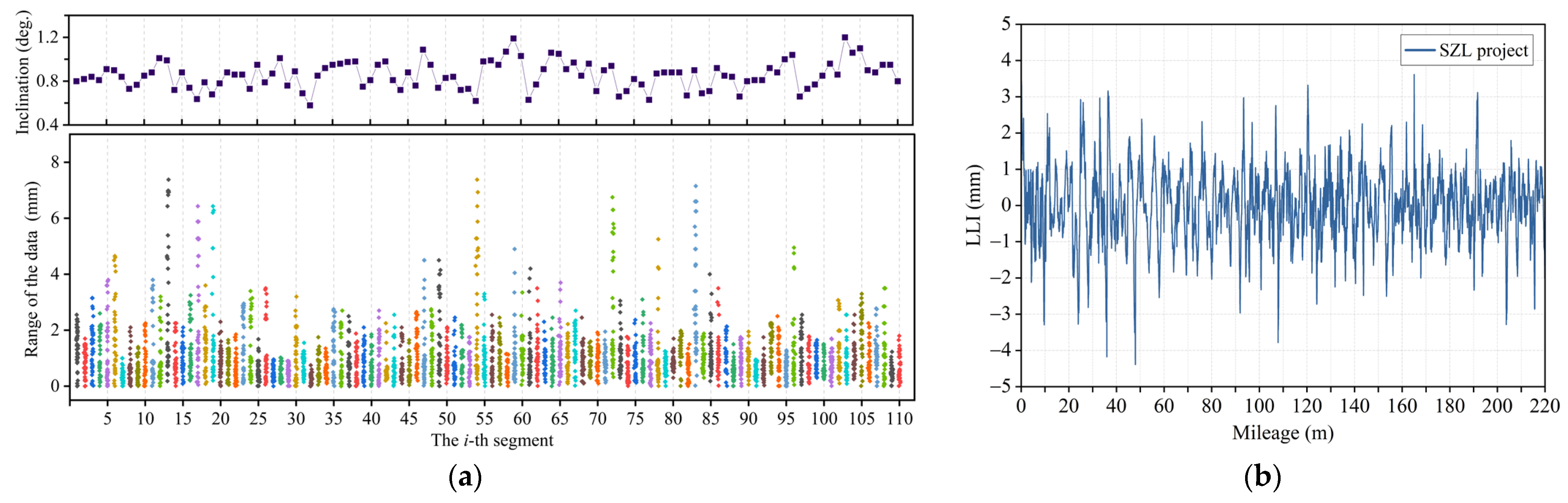
As a case study, we measured the LLI of the track beam of an MTTS project. The project is located in San-zhao-lun (SZL) city, China. The project adopts a steel box section for the track beam. The testing path, as we introduced, is the running path of the monorail vehicles; note that the slight difference in the width direction of the track beam is averaged by using the feeler gauge. The length of the level bar is 2 m, and the total measured length is 220 m with a sampling interval of 5 mm. The original data obtained by the inclinometer and feeler gauge are presented in Figure 15a. It can be observed that the range of data measured by the gauge feeler varies with the testing mileage of the track beam. As for the inclination obtained by the inclinometer, the measured values are all positive, mainly because a certain longitudinal grade was designed in the track beam. The distribution curve of the LLI of the track beam can be obtained, as shown in Figure 15b.

Figure 15.
(a) Original measured data of LLI. (b) Distribution curve of LLI after trend extraction.
In addition, considering the widely used CMM in railway systems, the measured data are analyzed in a general CMM manner by using the discussed approach of data extrapolation. To this end, the results of using TPOM and FPOM are explored. As shown in Equation (4), the transfer function of CMM is entirely dependent on the parametric setting. In addition, the change in parameters would make up distinctly different features of , such as the distribution of zero points and, more importantly, recoverable ranges of wavelength. The recoverable threshold of amplitude gains of is 0.1—to avoid abnormal restoration errors. After practical calculation, the parameters in Table 1 are selected. As shown in Table 1, FPOM can recover components of relatively shorter wavelengths, while TPOM provides a mildly higher value of the maximum recoverable range.

Table 1.
Selected value of parameters adopted in different types of CMMs.
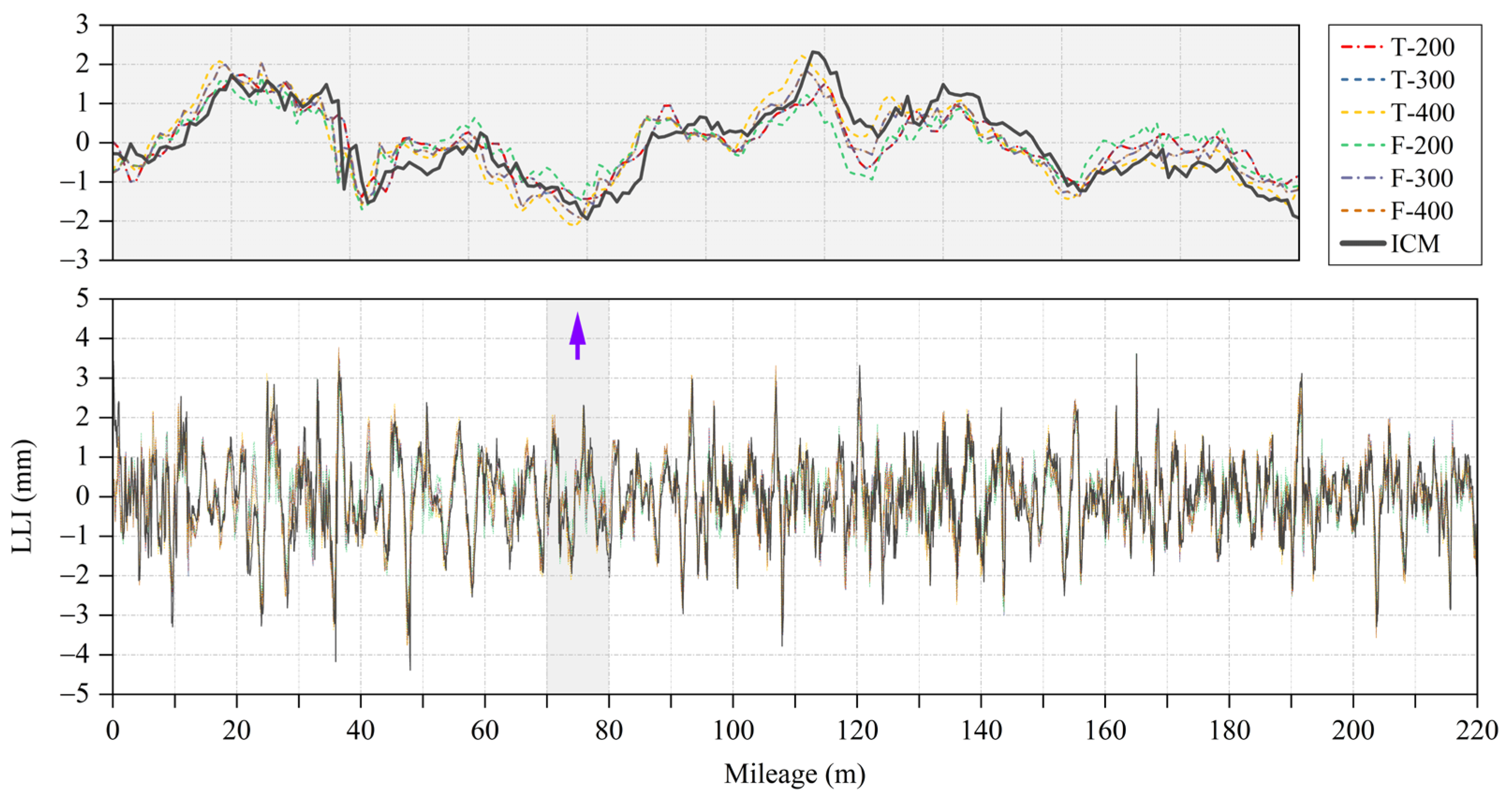
The restored distribution curves of LLI can be obtained after designing the corresponding inverse filters (Figure 14a) and filtering the extrapolated data, as shown in Figure 16. As shown, the distribution curves obtained by ICM and CMM are well consistent with each other, especially those obtained by CMMs. There are some fluctuations between the distribution curves obtained by ICM and those of CMM since the latter ignores certain components out of the recoverable range. In addition, mild differences between various types of CMMs can be observed, which means the selection of CMM types and parameters will affect the distribution curves of LLI to a certain extent. Note, the filtering process may have slightly affected the signal before that. The data analysis in ICM, however, does not need to take these into account.
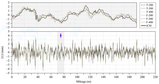
Figure 16.
Distribution curves of LLI obtained by various methods. T/F-200/300/400 means TPOM/FPOM with a/m = 200/300/400, see Table 1. The phase delay of CMM curves was eliminated in advance.
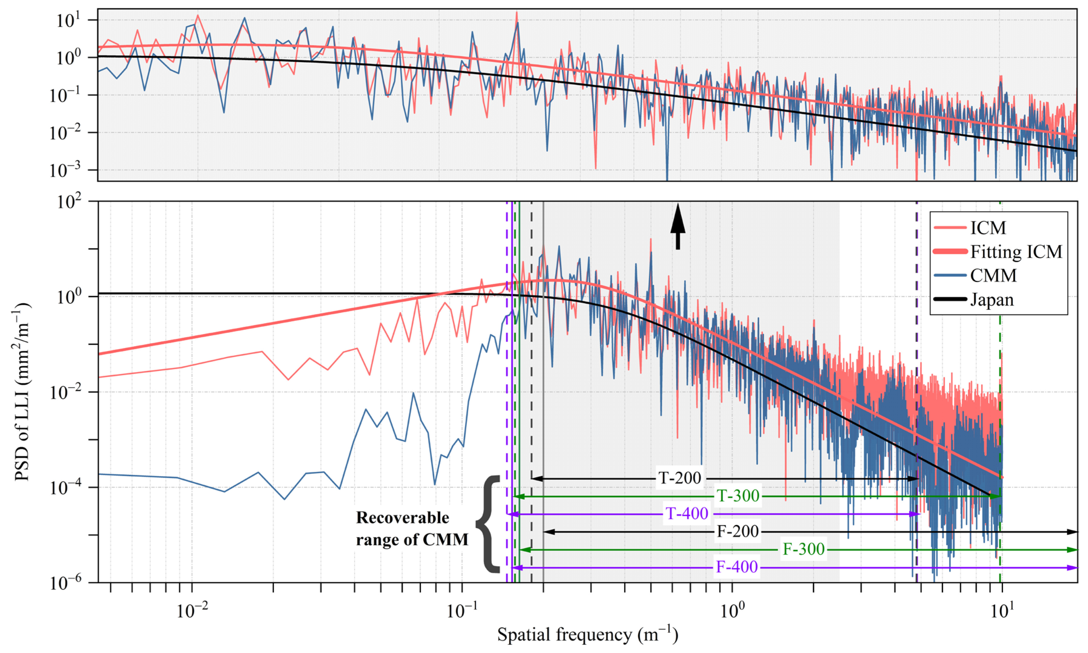
To better compare the performance of different methods, PSD curves are calculated to demonstrate the characteristic of LLI in the frequency domain. In addition, the form of PSD (or the spectrum) is beneficial to the subsequent application of track irregularity, including vibration tests of monorails, vehicle (-structure) systems, and engineering management. The classic method for spectral estimation called ‘Periodogram’ (see Equation (7)) is applied to obtain the PSD of distribution curves, as shown in Figure 17. In addition, the spectrum of the Japanese monorail [22], the most widely used spectrum for monorail systems thus far, is also included. Before estimation, the distribution curves of CMM are averaged to offset the differences caused by data filtering and parametric selection. The sampling frequency is 20 Hz in this case. Therefore, wavelengths below 0.1 m are not considered. Nevertheless, ICM can consider a broader frequency range theoretically once the sampling frequency is increased. Furthermore, an improved fractional function (see Equation (8)) is used to fit the estimated spectrum and obtain the results of , , and .
where , , , , and are the estimated value, sampling frequency, sample length, sampling period, and the input of a discrete time series, respectively.
where , , and are parameters to be fitted, is the PSD, and is the spatial frequency, Hz.

Figure 17.
PSD of the distribution curves of LLI obtained by ICM and CMM, the Japanese monorail, and the fitting result of ICM. Note, the curve of CMM is the average value of six CMM sequences of different parameters; the curve of ICM is fitted by Equation (8) with parameters of A = 0.11, B = 0.28, and n = 3.83; in addition, the recoverable ranges of different CMM are denoted.
The results in Figure 17 demonstrate that whether it is within the recoverable range or not, the overall characteristics of the PSD of LLI measured by ICM and CMM are consistent with each other, although there is certain fluctuation in the PSD values, which verifies the correctness of proposed methods. For CMM, the magnitude of the PSD is distorted because of the unreal time/mileage curve. Significant differences in the magnitude can be found between the PSD obtained by ICM and CMM in the medium- and long-wave area (about 5 to 200 m). Specifically, as Table 1 shows, the magnitude of the transfer function of CMM is too small to be recovered from 5.535 m, 6.369 m, etc. In addition, the comparison between the measured PSDs with the Japanese spectrum shows that more attention should be paid to the low-frequency or long-wavelength range (lower than 12.5 m) of track irregularity. For example, track irregularity is adopted in high-frequency vibration test of vehicle components. Note that in the long-wave ranges, the measured PSD value in this work is approximate to that of the original data of the Japanese monorail. After curve fitting conducted in [22], however, the magnitude of its PSD value is relatively overestimated.
3.3. Numerical Simulation Using Multi-Body Dynamics
To further demonstrate the significance of the obtained results, including the measured data and related spectrum of track irregularity, a numerical simulation is presented in this section. The simulation is conducted by using a joint model based on multi-body dynamics (MBD) and the finite element method (FEM). MBD is utilized to simulate the monorail vehicle via SIMPACK (2021x), while FEM is employed to simulate the track beam via ANSYS software (19.2). Afterward, the established model of the track beam is transferred into SIMPACK and serves as a flexible body. The coupling between the vehicle and track beam is then realized using move markers. Extensive studies have proven the effectiveness of using a joint MBD-FEM model for the simulation of vehicle–track interactions in various transportation systems including monorails [32,33,34].
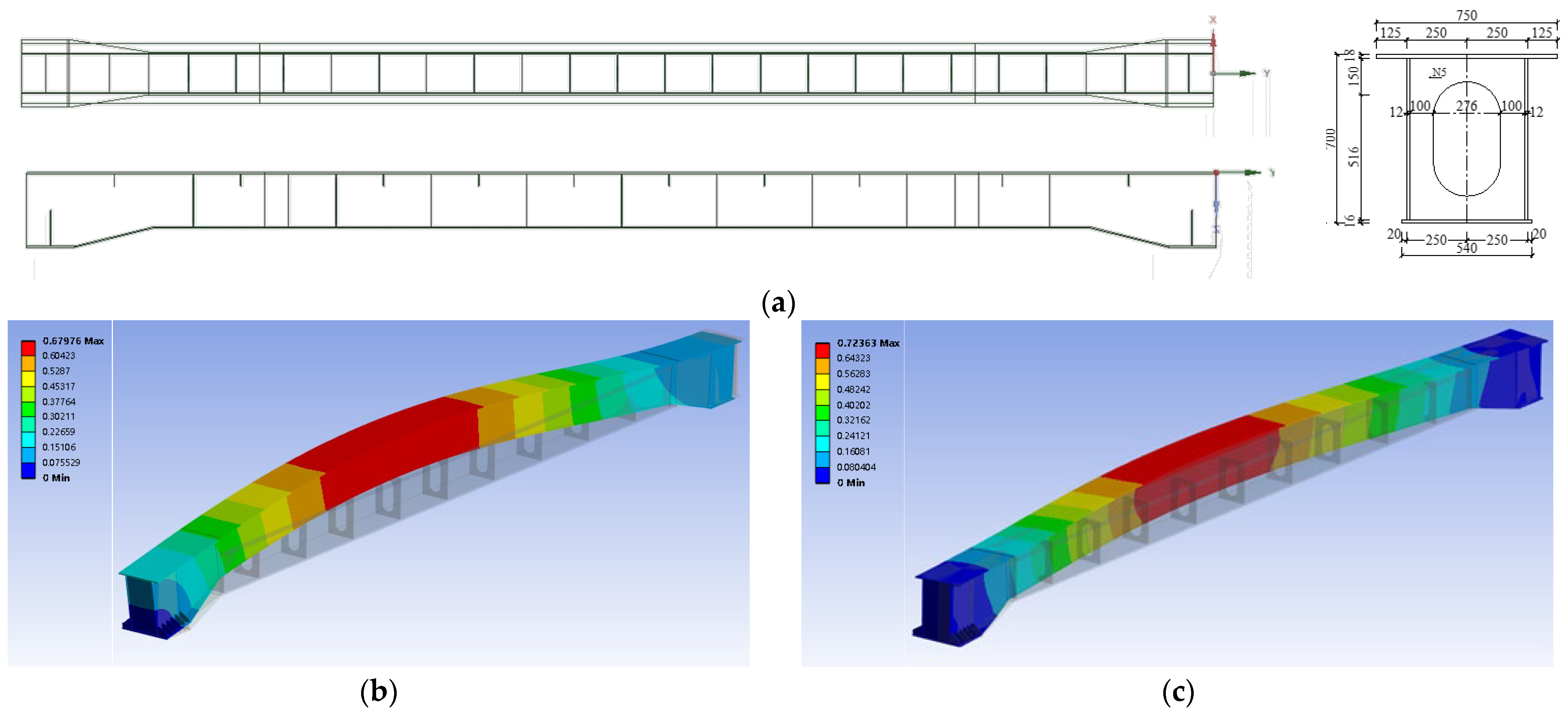
Regarding the modeling, a 15 m long steel track beam is modeled using a solid element; minor details such as the upper stiffener are not considered as long as the overall stiffness is consistent with the actual one. The general configuration of the track beam is shown in Figure 18a; more details can be found in the Supplementary Files. A modal analysis is then conducted, and the results of the first four deformed shapes are plotted in Figure 18b,c.
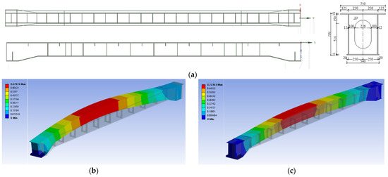
Figure 18.
Configuration of the modeled track beam and the results of modal analysis. (a) General configuration of the track beam to be modeled. (b) Mode 1, 14.39 Hz. (c) Mode 2, 15.27 Hz.
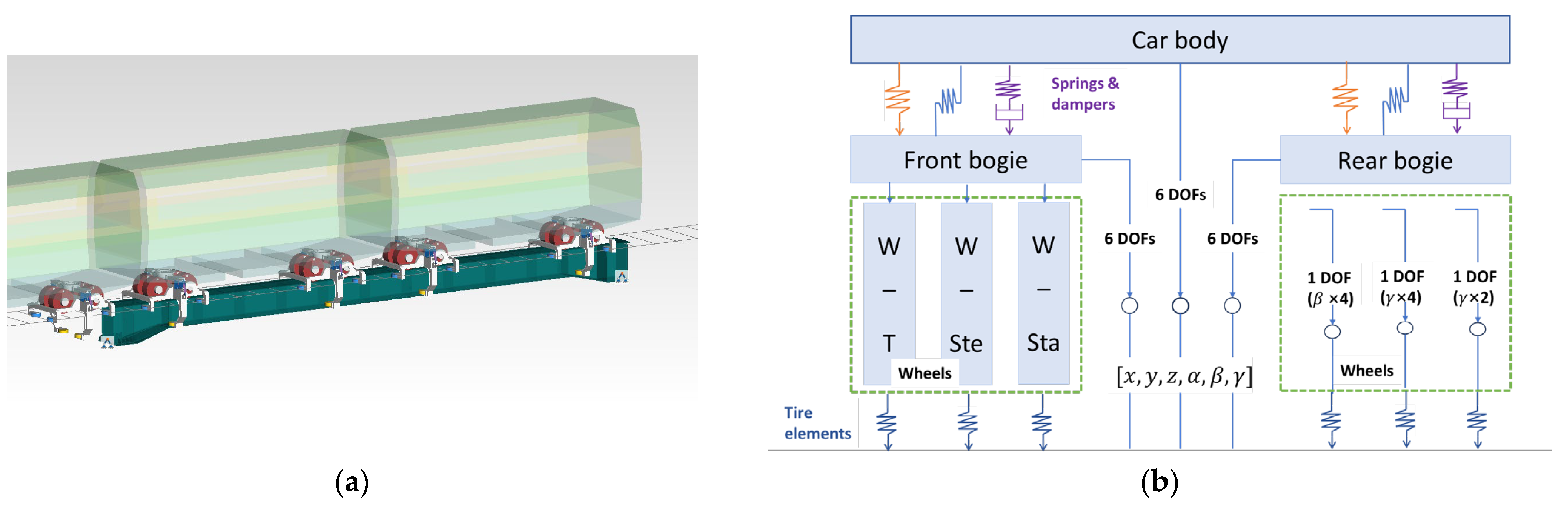
As for the modeling of the monorail train, all the major components of the train are simulated as separate rigid objects and connected to the other objects through mechanical joints or constraints that define their relative motion. The monorail train generally contains many identical carriages and hence, each carriage can be modeled as a substructure and assembled directly into the vehicle system. Likewise, each bogie is a substructure of the carriage, and the wheels are the substructure of the bogie. The major configuration of the vehicle bogie is shown in Figure 1, the assembled train model and the transferred model of the track beam are shown in Figure 19, and details about the train model can be found in the Supplementary Files.
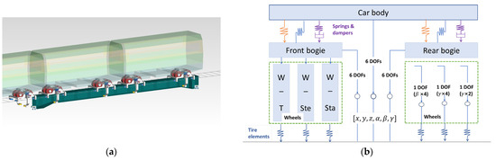
Figure 19.
Joint MBD-FEM model. Note, W_T/Ste/Sta are the traveling/steering/stabilizing wheels, and their numbers on each bogie are 4, 4, and 2, respectively. (a) A monorail train running on the track beam. (b) Topology of the carriage of the modeled train.
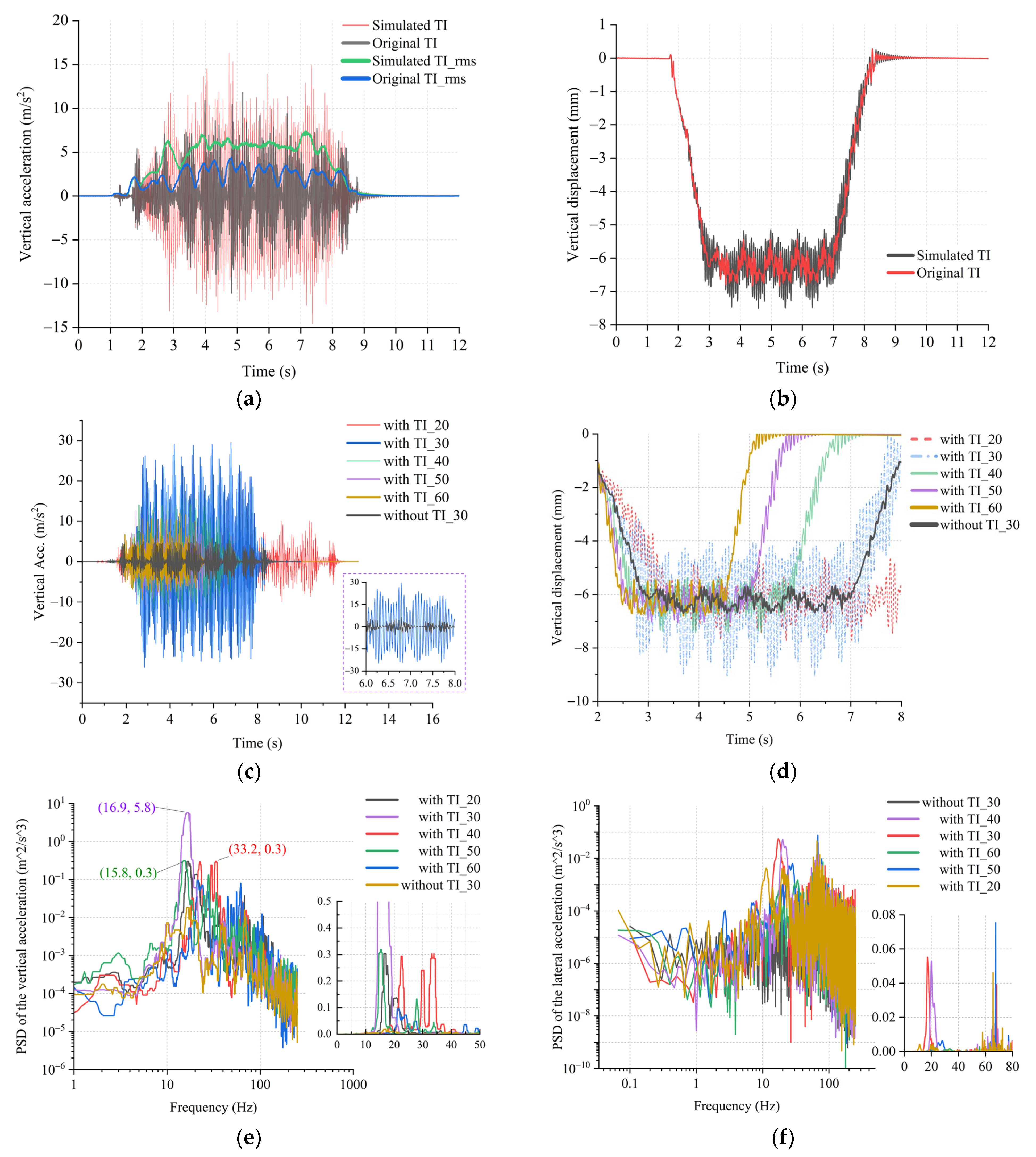
To verify the established model, a field dynamic test was conducted in an MTTS project. In this test, the dynamic displacement of the track beam at the mid-span was obtained by using a linear variable differential transformer (LVDT), as shown in Figure 20a. It should be noted that the measured track irregularity was applied during the simulation (original TI in Figure 20b). Time integration was then conducted in SIMPACK with the vehicle speed of 30 km/h, and the results obtained by the model and field test are illustrated in Figure 20c. As shown, the overall simulation result is highly consistent with the test. The simulated result is able to capture the skeleton of the time history curve of the vertical displacement and reflect the impact of the carriage sequence, although the transferred model of the track beam exhibits a slightly lower stiffness. The overall condition of the track condition is good because the measurement was performed shortly after the project was completed. Hence, the effect of track irregularity on the displacement of the track beam is not significant. However, the applied track irregularity still induced significant effects on the vibration of the monorail train under different running speeds. As shown in Figure 20d, the vehicle body experiences approximately twice the maximum vertical acceleration when accounting for track irregularity.
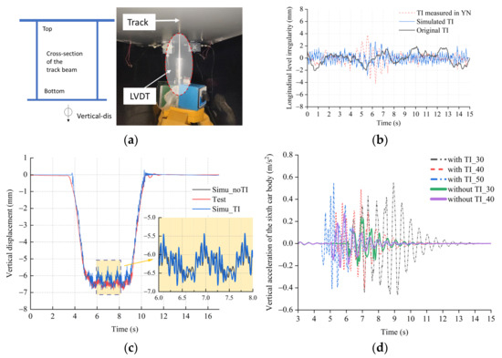
Figure 20.
Verification of the model and the responses of MTTS train and track. The simulated TI is generated based on the data measured in the YN project located in Yunnan, China. Note, TI_30 means the running speed is 30 km/h with the existence of track irregularity. (a) Set up of the field test. (b) Track irregularity used in the model. (c) Comparison of displacement. (d) Comparison of acceleration.
Moreover, to examine the sensitivity of the dynamic response to the track irregularity, a track irregularity sequence measured in another project was chosen and used to generate a simulated sequence with a similar amplitude level compared to the original sequence, as shown in Figure 20b. Figure 21 illustrates the results of the dynamic responses under various track conditions and running speeds. As shown, although having similar levels of irregularity amplitude, the dynamic responses are much more significant under the simulated track irregularity, which is believed to be due to the characteristics in the frequency domain. A more detailed simulation process was conducted under the measured signal in the YN project. The results indicated that the dynamic response does not strictly follow the increase in the running speeds but achieves the maximum value at the speed of 30 km/h rather than 50 km/h or 60 km/h. Under the same parameters of the structure (e.g., wheelbase, length of the car body), the change in running speed directly affects the induced frequency of the track beam. Observation of the PSD curves of the acceleration response indicates that the main frequency induced by the train with a speed of 30 km/h is 16.9 Hz, which is close to the natural frequency of the track beam and one of the main frequencies of track irregularity data. Of course, more efforts should be made to provide a more credible explanation for this phenomenon. Nevertheless, we can still conclude that MTTS is sensitive to the frequency information of track irregularity and hence, it is of great value to obtain a high-precision dataset, including the distribution curve and its spectrum of track irregularity.
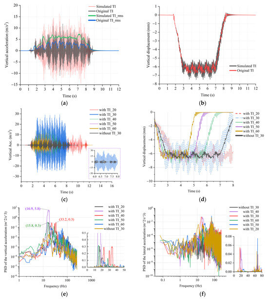
Figure 21.
Dynamic responses of the track beam under various track conditions and running speeds. (a,b) Results of vertical acceleration and displacement under original and simulated track irregularities. Note, rms is the moving root-mean-square value calculated with a window size of 50; Results in (c–f) are simulated under the measured track irregularity from the YN project.
In summary, the results of the case study are coincident with the field tests, simulation, and theoretical analysis, and all indicate the potential value of the proposed methods. The comparison of PSD curves shows the advantages of ICM in the available frequency range and precision level, which are meaningful to its engineering applications because different systems are sensitive to diverse wavelengths of excitation. In addition, the proposed method is applicable for the design of automatic measuring systems since it adopts a distinct principle, thereby proving higher efficiency in the measuring process. The established MBD-FEM model demonstrates the great effects of track irregularity on the dynamic responses of MTTS and reveals the importance of using an accurate signal of track irregularity and its spectrum in the dynamic studies of MTTS.
4. Conclusions
In this work, to address the lagging research on the track irregularity of monorail systems, we explore the effectiveness of using ICM to measure track irregularity conveniently and introduce an adaptive method for its trend extraction before subsequent spectral analysis. The principle of ICM as well as its relationship to the conventionally used CMM is revealed. All proposed methods are carefully examined and verified under computer simulation. Afterwards, a case study including the field measurement of LLI and a numerical simulation in an MTTS project is performed. The comparison of data obtained in the simulation and case study are consistent, both indicating the accuracy, robustness, and advantages of the proposed methods. The main conclusions are as follows:
- The proposed ICM is derived from general chord-based methods and can maintain the initial baseline by utilizing inclination data, thereby obtaining an authentic waveform of track irregularity. Hence, it has advantages in waveform fidelity, recoverable range of wavelength, and resistance to interference parametric selection. In addition, it has the potential to be integrated into current chord-based systems conveniently.
- All the measurement and signal processing methods were successfully validated by computer simulations. Simulations of using ICM at predetermined errors demonstrated its accuracy and robustness both qualitatively and quantitatively. The RMS values of the ICM measurement differences were 3.58 × 10⁻⁴, 0.31, 0.59, and 0.856 mm (under an actual, 1, 3, and 5 times the nominal error), respectively, compared with an averaged value of 1.27 mm for CMM.
- An adaptive method for trend extraction was summarized as follows: decomposing signals by CEEMDAN and identifying trend components based on HMS. Calculation proved that such a combination improves the performance of signal decomposition, thereby enhancing the quality of trend identification and subsequent spectral estimation, especially for those nonstationary signals with trend items of high amplitude.
- The longitudinal level irregularity of an MTTS project was successfully measured and a high-precision spectrum was obtained. Comparison of results further proves ICM in obtaining the actual value and corresponding high-precision PSD of track irregularity. Results show that more attention should be paid to LLI with a wavelength smaller than 12.5 m when adopting the Japanese spectrum. A more recommended spectrum is provided by .
- The results of the numerical simulation indicate that both the amplitude and the frequency features are essential for the evaluation of the dynamic responses of MTTS. Under the excitation of track irregularity, the fluctuation amplitude of the simulated vertical displacement and the maximum acceleration response can even reach two to three times the original amplitude.
Supplementary Materials
The following supporting information can be downloaded at: https://www.mdpi.com/article/10.3390/math12142197/s1, S1: Modelling details of the track beam; S2: Modelling the monorail train.
Author Contributions
Conceptualization, methodology, and writing—original draft, P.W. and F.G.; data curation and formal analysis, P.W.; funding acquisition and supervision, F.G.; investigation and software, P.W. and H.Z.; project administration, F.G., J.J., Q.L. and Y.Y.; resources, F.G., H.Z., J.J., Q.L. and Y.Y.; Validation and writing—review and editing, all authors. All authors have read and agreed to the published version of the manuscript.
Funding
This research was funded by Zhuzhou CRRCTK under project No: 738011925, focused on the development of the Monorail Elevated Steel Structure Rapid Transit System.
Data Availability Statement
The original contributions presented in the study are included in the article and Supplementary Material, further inquiries can be directed to the corresponding author.
Acknowledgments
The authors thank the support from the technicians of the Zhuzhou CRRC Special Equipment Tech. Co., Ltd., in the field tests.
Conflicts of Interest
Authors Junhui Jin, Qiaoyun Liao and Yongfeng Yan were employed by Zhuzhou CRRC Special Equipment Technology Co. The remaining authors declare that the research was conducted in the absence of any commercial or financial relationships that could be construed as a potential conflict of interest.
Abbreviations
The following abbreviations are used in this manuscript:
| CEEMDAN: | complete ensemble empirical mode decomposition with adaptive noise |
| CMM: | chord measuring method |
| EMD: | empirical mode decomposition |
| FEM: | finite element method |
| FIR: | finite impulse response |
| FPOM: | four-point offset method |
| HMS: | Hilbert marginal spectrum |
| IMF: | intrinsic mode function |
| IRM: | inertial reference method |
| LLI: | longitudinal level irregularity |
| MBD: | multi-body dynamics |
| MTTS: | monorail tour-transit systems |
| PSD: | power spectral density |
| RMS: | root-mean-square |
| RSS: | residual sum of squares |
| SZL: | San-zhao-lun (city name) |
| TPOM: | three-point offset method |
References
- Hettiarachchi, C.; Yuan, J.; Amirkhanian, S.; Xiao, F. Measurement of pavement unevenness and evaluation through the IRI parameter—An overview. Measurement 2023, 206, 112284. [Google Scholar] [CrossRef]
- Munoz, S.; Urda, P.; Yu, X.; Mikkola, A.; Escalona, J.L. Real-Time Measurement of Track Irregularities Using an Instrumented Axle and Kalman Filtering Techniques. J. Comput. Nonlinear Dyn. 2023, 18, 111005. [Google Scholar] [CrossRef]
- Matsuoka, K.; Tanaka, H. Drive-by deflection estimation method for simple support bridges based on track irregularities measured on a traveling train. Mech. Syst. Signal Process. 2023, 182, 109549. [Google Scholar] [CrossRef]
- Zhang, T. APM and Monorail for urban applications. In Proceedings of the Automated People Movers and Automated Transit Systems, Toronto, ON, Canada, 17–20 April 2016; pp. 222–239. [Google Scholar]
- Timan, P.E. Why monorail systems provide a great solution for metropolitan areas. Urban Rail Transit 2015, 1, 13–25. [Google Scholar] [CrossRef]
- Cantero, D.; Karoumi, R. Numerical evaluation of the mid-span assumption in the calculation of total load effects in railway bridges. Eng. Struct. 2016, 107, 1–8. [Google Scholar] [CrossRef]
- Naeimi, M.; Zakeri, J.A.; Esmaeili, M.; Mehrali, M. Dynamic response of sleepers in a track with uneven rail irregularities using a 3D vehicle–track model with sleeper beams. Arch. Appl. Mech. 2015, 85, 1679–1699. [Google Scholar] [CrossRef]
- Zhou, J.; Du, Z.; Yang, Z.; Xu, Z. Dynamic parameters optimization of straddle-type monorail vehicles based multiobjective collaborative optimization algorithm. Veh. Syst. Dyn. 2019, 3, 357–376. [Google Scholar] [CrossRef]
- Tsai, H.C.; Wang, C.Y.; Huang, N.E.; Kuo, T.W.; Chieng, W.H. Railway track inspection based on the vibration response to a scheduled train and the Hilbert–Huang transform. Proc. Inst. Mech. Eng. Part F J. Rail Rapid Transit 2015, 229, 815–829. [Google Scholar] [CrossRef]
- Tanaka, H.; Shimizu, A. Practical application of portable trolley for the continuous measurement of rail surface roughness for rail corrugation maintenance. Q. Rep. RTRI 2016, 57, 118–124. [Google Scholar] [CrossRef]
- Jeong, W. Spectral Characteristics of Rail Surface by Measuring the Growth of Rail Corrugation. Appl. Sci. 2021, 11, 9568. [Google Scholar] [CrossRef]
- Peng, L.; Zheng, S.; Li, P.; Wang, Y.; Zhong, Q. A comprehensive detection system for track geometry using fused vision and inertia. IEEE Trans. Instrum. Meas. 2020, 70, 1–15. [Google Scholar] [CrossRef]
- Lee, J.S.; Choi, S.; Kim, S.S.; Park, C.; Kim, Y.G. A mixed filtering approach for track condition monitoring using accelerometers on the axle box and bogie. IEEE Trans. Instrum. Meas. 2011, 61, 749–758. [Google Scholar] [CrossRef]
- Lathe, A.S.; Gautam, A. Estimating vertical profile irregularities from vehicle dynamics measurements. IEEE Sens. J. 2019, 20, 377–385. [Google Scholar] [CrossRef]
- Shi, J.; Fang, W.S.; Wang, Y.J.; Zhao, Y. Measurements and analysis of track irregularities on high speed maglev lines. J. Zhejiang Univ. Sci. A 2014, 15, 385–394. [Google Scholar] [CrossRef]
- Salvador, P.; Naranjo, V.; Insa, R.; Teixeira, P. Axlebox accelerations: Their acquisition and time–frequency characterisation for railway track monitoring purposes. Measurement 2016, 82, 301–312. [Google Scholar] [CrossRef]
- Zhang, S.; Kang, X.; Liu, X. Characteristic analysis of the power spectral density (PSD) of track irregularity on Beijing-Tianjin inter-city railway. China Railw. Sci. 2008, 29, 25–30. [Google Scholar]
- Wang, Y.; Tang, H.; Wang, P.; Liu, X.; Chen, R. Multipoint chord reference system for track irregularity: Part I—Theory and methodology. Measurement 2019, 138, 240–255. [Google Scholar] [CrossRef]
- Wang, Y.; Tang, H.; Wang, P.; Liu, X.; Chen, R. Multipoint chord reference system for track irregularity: Part II—Numerical analysis. Measurement 2019, 138, 194–205. [Google Scholar] [CrossRef]
- Guo, F.; Chen, K.; Gu, F.; Wang, H.; Wen, T. Reviews on current situation and development of straddle-type monorail tour transit system in China. J. Cent. South Univ. Sci. Technol. 2021, 52, 4540–4551. [Google Scholar]
- Guo, F.; Wang, P. Measurement and analysis of the longitudinal level irregularity of the track beam in monorail tour-transit systems. Sci. Rep. 2022, 12, 19219. [Google Scholar] [CrossRef]
- Lee, C.H.; Kawatani, M.; Kim, C.W.; Nishimura, N.; Kobayashi, Y. Dynamic response of a monorail steel bridge under a moving train. J. Sound Vib. 2006, 294, 562–579. [Google Scholar] [CrossRef]
- Gou, H.; Zhou, W.; Yang, C.; Bao, Y.; Pu, Q. Dynamic response of a long-span concrete-filled steel tube tied arch bridge and the riding comfort of monorail trains. Appl. Sci. 2018, 8, 650. [Google Scholar] [CrossRef]
- Kim, Y.S.; Lim, T.K.; Park, S.H.; Jeong, R.G. Dynamic model for ride comfort evaluations of the rubber-tired light rail vehicle. Veh. Syst. Dyn. 2008, 46, 1061–1082. [Google Scholar] [CrossRef]
- Yu, Z.W.; Mao, J.F. A stochastic dynamic model of train-track-bridge coupled system based on probability density evolution method. Appl. Math. Model. 2018, 59, 205–232. [Google Scholar] [CrossRef]
- Wu, Z.; Huang, N.E. Ensemble empirical mode decomposition: A noise-assisted data analysis method. Adv. Adapt. Data Anal. 2009, 1, 1–41. [Google Scholar] [CrossRef]
- Zhang, J.; Pan, Z.X.; Zheng, Y.X.; Li, Y. Research on vibration signal trend extraction. Acta Electron. Sin. 2017, 45, 22–28. [Google Scholar]
- Lu, S.; Wang, X.; Yu, H.; Dong, H.; Yang, Z. Trend extraction and identification method of cement burning zone flame temperature based on EMD and least square. Measurement 2017, 111, 208–215. [Google Scholar] [CrossRef]
- Yang, Z.; Ling, B.W.K.; Bingham, C. Trend extraction based on separations of consecutive empirical mode decomposition components in Hilbert marginal spectrum. Measurement 2013, 46, 2481–2491. [Google Scholar] [CrossRef]
- Colominas, M.A.; Schlotthauer, G.; Torres, M.E. Improved complete ensemble EMD: A suitable tool for biomedical signal processing. Biomed. Signal Process. Control. 2014, 14, 19–29. [Google Scholar] [CrossRef]
- Yoshimura, A. Theory and practice for restoring an original waveform of a railway track irregularity. Railw. Tech. Res. Inst. Q. Rep. 1995, 36, 85–94. [Google Scholar]
- Bosso, N.; Zampieri, N. Long train simulation using a multibody code. Veh. Syst. Dyn. 2017, 55, 552–570. [Google Scholar] [CrossRef]
- Lovisa, A.C.; Garack, O.; Clarke, J.; Michael, M. A workflow for the dynamic analysis of freight cars using Simpack. In Dynamics of Vehicles on Roads and Tracks; CRC Press: Boca Raton, FL, USA, 2017; Volume 2, pp. 1297–1302. [Google Scholar]
- Li, Y.; Xu, X.; Zhou, Y.; Cai, C.S.; Qin, J. An interactive method for the analysis of the simulation of vehicle–bridge coupling vibration using ANSYS and SIMPACK. Proc. Inst. Mech. Eng. Part F J. Rail Rapid Transit 2018, 232, 663–679. [Google Scholar] [CrossRef]


Disclaimer/Publisher’s Note: The statements, opinions and data contained in all publications are solely those of the individual author(s) and contributor(s) and not of MDPI and/or the editor(s). MDPI and/or the editor(s) disclaim responsibility for any injury to people or property resulting from any ideas, methods, instructions or products referred to in the content. |
© 2024 by the authors. Licensee MDPI, Basel, Switzerland. This article is an open access article distributed under the terms and conditions of the Creative Commons Attribution (CC BY) license (https://creativecommons.org/licenses/by/4.0/).