
An Innovative Method for Deterministic Multifactor Analysis Based on Chain Substitution Averaging


Abstract
1. Introduction
- additive or different models—in them, the performance indicator is the sum or difference of the factor variables involved, namely:
- multiplicative models—here, the performance indicator is the product of the factor variables involved, namely: ;
- multiple model—here, the performance indicator is the quotient of the factor variables involved, namely: ;
- mixed (combined) models—these are combinations of additive or different, multiplicative or multiple factor models and can be as follows: multiplicative-multiple, additive or different-multiple, additive or different-multiplicative, and additive or different-multiplicative-multiple models.
2. Applicability of Deterministic Factor Analysis Methods to the Types of Factor Model
3. Research Methods and Methodology of the Averaged Chain Substitution Method
- (1)
- The type of factor model is two-factor multiplicative;
- (2)
- The number of factor variables involved is two;
- (3)
- The number of possible combinations of the order of substitution of the factor variables is two (), namely: and ;
- (4)
- Construction of the factor chains after the method of chain substitutions in the order of substitution of factor variables in the factor chains, i.e., first then . This is carried out according to the following expressions:
- (5)
- Determining the influence of factor in a substitution of the type a − b in a substitution of the type:
- (6)
- Determining the influence of factor b in a substitution of the type a − b after this expression:
- (7)
- Construction of the factor chains after the method of chain substitutions in the order of substitution of factor variables в in the factor chains, i.e., first then . This is carried out according to the following expressions:
- (8)
- Determining the influence of factor in a substitution of the type following the expression below:
- (9)
- Determining the influence of factor in a substitution of the type after this expression:
- (10)
- Determining the averaged influence of factor after this expression:
- (11)
- Determining the averaged influence of factor after the expression:
- for factor :
- for factor :
- (1)
- The type of factor model is two-factor multiple;
- (2)
- The number of factor variables involved is two;
- (3)
- The number of possible combinations of the order of substitution of the factor variables is two (), namely: and ;
- (4)
- Construction of the factor chains after the method of chain substitutions in the order of substitution of factor variables in the factor chains, i.e., first then . This is carried out according to the following expressions:
- (5)
- Determining the influence of factor in a substitution of the type following the expression:
- (6)
- Determining the influence of factor in a substitution of the type after this expression:
- (7)
- Construction of the factor chains after the method of chain substitutions in the order of substitution of factor variables in the factor chains, i.e., first then . This is carried out according to the following expressions:
- (8)
- Determining the influence of factor in a substitution of the type following the expression below:
- (9)
- Determining the influence of factor in a substitution of the type after this expression:
- (10)
- Determining the averaged influence of factor after this expression:
- (11)
- Determining the averaged influence of factor after the expression:
- for factor :
- for factor :
4. Systematization of the Results of the Approbation of the Averaged Chain Substitution Method
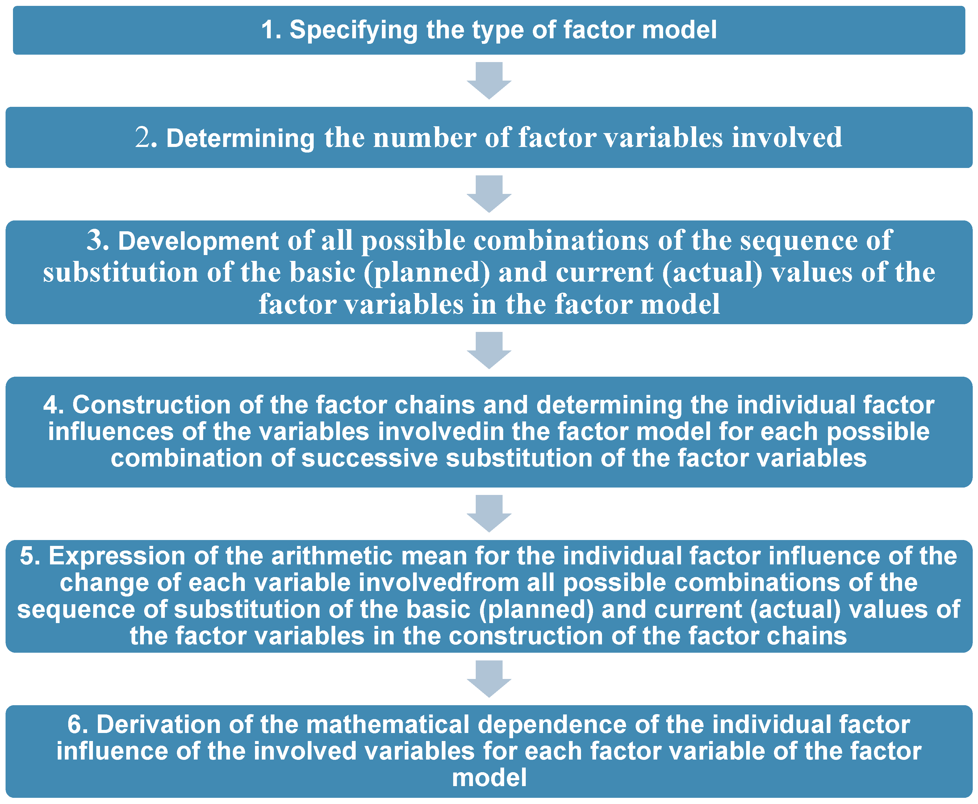
5. Derivation of Individual Factor Influences for Five-Factor Models
6. Dynamic DFA by the Averaged Chain Substitution Method—Examples
- —the value of current receivables for the period , in BGN thousands;
- —the value of current financial assets for the period , in BGN thousands;
- —the value of cash and cash equivalents for the period , in BGN thousands;
- —the value of current liabilities for the period , in BGN thousands;
- —the index of the th value of the performance indicator and of the participating factor variables over time, .
- for a factor value of inventories :
- for a factor value of short-term receivables :
- for a factor value of current financial assets :
- for a factor value of cash and cash equivalents :
- for a factor value of current liabilities :
7. Discussion
8. Conclusions
Author Contributions
Funding
Data Availability Statement
Acknowledgments
Conflicts of Interest
References
- Jugenburg, S.M. On the Question of the Expansion of the Absolute Increase in Factors. In Scientists Note on Statistics = Uchenye Zapiski po Statistike; Izd-vo Akademii nauk SSSR: Moscow, Russia, 1955; Volume 3, pp. 372–376. [Google Scholar]
- Humal, A. Separation of the Growth of the Multiplication. In Scientists Note on Statistics = Uchenye Zapiski po Statistike; Izd-vo Akademii nauk SSSR: Moscow, Russia, 1964; Volume 8, pp. 206–212. [Google Scholar]
- Fedorova, V.I.; Egorov, Y. On the Question of the Expansion of Growth Factors on. In Statistics Herald = Vestnik Statistiki; Izd-vo Gostizdat SSSR: Moscow, Russia, 1977; Volume 5, pp. 71–73. [Google Scholar]
- Sheremet, A.D.; Djej, G.G.; Shapovalov, V.N. Method of Chain Substitutions and Improvement Factor Analysis of Economic Indicators. In Bulletin of Moscow State University Ser. 6: “Economy”; Moskovskiy gosudarstvennyy universitet imeni Lomonosova SSSR: Moscow, Russia, 1971; Volume 4, pp. 62–69. [Google Scholar]
- Adamov, V.E. Factor Index Analysis (Methodology and Problems); Politizdat: Moscow, Russia, 1977. [Google Scholar]
- Lipovetsky, S.S. Variational analysis of the distribution of growth by disease. In Economics and Mathematical Methods; Izd-vo Akademii nauk SSSR: Moscow, Russia, 1983; Volume 1, pp. 125–130. [Google Scholar]
- Vaninskiy, A.Y. Integral Method of Economic Analysis in the Historical and Methodological Aspect. In Bulletin of Moscow State University Ser. 6: “Economy”; Moskovskiy gosudarstvennyy universitet imeni Lomonosova SSSR: Moscow, Russia, 1987; Volume 1, pp. 34–41. [Google Scholar]
- Foster, G. Financial Statement Analysis, 2nd ed.; Prentice-Hall: Englewood Cliffs, NJ, USA, 1986. [Google Scholar]
- Bernstein, L.A.; Wild, J.J.; Subramanyam, K.R. Financial Statement Analysis, 7th ed.; McGraw-Hill: Irwin, CA, USA, 2001. [Google Scholar]
- Ross, S.A.; Westerfield, R.W.; Jaffe, J.F. Corporate Finance, 2nd ed.; Irwin: Homewood, IL, USA, 1990. [Google Scholar]
- Emery, D.R.; Finnerty, J.D.; Stowe, J.D. Corporate Financial Management, 2nd ed.; Prentice-Hall: Englewood Cliffs, NJ, USA, 2004. [Google Scholar]
- Bakanov, M.I.; Sheremet, A.D. Theory of Economic Analysis, 4th ed.; Finance and Statistics: Moscow, Russia, 2001. [Google Scholar]
- Chebotarev, S.V. Lagrange′s Method and the Budan-Fourier Theorem in Economic Factor Analysis. In Automation and Remote Control = Sistemy Upravlenija i Informacionnye Tehnologii; Izd-vo Nauchna kniga: Mosco-Voronej, Russia, 2003; Volume 1, pp. 30–35. [Google Scholar]
- Kremer, N.S. Higher Mathematics for Economic Specialties; Higher Education: Moscow, Russia, 2005. [Google Scholar]
- Lyubushin, N.P. Analysis of the Financial and Economic Activities of the Enterprise; UNITI-DANA: Moscow, Russia, 2009. [Google Scholar]
- Lebedev, K.N. The Problem of Factor Analysis Based on Deterministic Methods of Factor Analysis (Problems of Science “Economic Analysis). Econ. Theory Anal. Pract. 2012, 3, 4–13. [Google Scholar]
- Prokofiev, V.A.; Nosov, V.V.; Salomatina, T.V. Preconditions and Conditions for the Development of Deterministic Factor Analysis (Problems of the Science of “Economic Analysis”). Econ. Theory Anal. Pract. 2014, 4, 134–145. [Google Scholar]
- Savitskaya, G.V. The Theory of the Analysis of Economic Activity; IMFRA-M: Moscow, Russia, 2012. [Google Scholar]
- Mitev, V.T. The Method of Chain Substitutions—Practical Application in Financial Business Analysis: Advantages and Shortcomings. Annu. Univ. Min. Geol. “St. Ivan Rilski” 2008, 51, 45–48. [Google Scholar]
- Mitev, V.T. Averaged Chain Substitution Method. In Economic and Social Alternatives = Ikonomiceski i Sotsialni Alternativi; Universitet za nacionalno i svetovno stopanstvo: Sofia, Bulgaria, 2020; Volume 4, pp. 90–100. [Google Scholar] [CrossRef]
- Mitev, V.T. Averaged Chain Substitution Method—Applicability, Advantages, and Disadvantages. In Economic and Social Alternatives = Ikonomiceski i Sotsialni Alternativi; Universitet za nacionalno i svetovno stopanstvo: Sofia, Bulgaria, 2021; Volume 2, pp. 127–138. [Google Scholar] [CrossRef]
- Mitev, V.T. Approbation of the averaged method of chain substitutions for three- and four-multiples and multiplicative-multiples factor models. Financ. Theory Pract. 2022, 26, 166–174. [Google Scholar] [CrossRef]
- Mitev, V.T. Dynamic Deterministic Factor Analysis Using the Averaged Chain Substitution Method. Economic and Social Alternatives = Ikonomiceski i Sotsialni Alternativi; Universitet za nacionalno i svetovno stopanstvo: Sofia, Bulgaria, 2023; Volume 1, pp. 131–148. [Google Scholar] [CrossRef]

| Methods of DFA | Types of Factor Models | |||
|---|---|---|---|---|
| Additive or Different | Multiplicative | Multiple | Mixed | |
| Differential method | − | + | − | − |
| Coefficient method | − | + | − | − |
| Chain substitution method | + | + | + | + |
| Index method | − | + | + | − |
| Absolute difference method | − | + | − | Only when |
| Absolute relative method | − | + | − | Only when |
| Equity participation method | − | + Only when | − | − |
| The method of simple addition of an indecomposable remainder | − | + | − | − |
| Weighted finite difference method | − | + | − | − |
| The method of increment division into factors | − | + | − | − |
| Integral method | − | + | + | Only when |
| Logarithmic method | − | + Only when ∆P ≠ 0 | + Only when | Only when and |
| Factor Models, (Limitation) | ||||
|---|---|---|---|---|
| Multiplicative Factor Models | ||||
| - | - | |||
| - | ||||
| Additive-Multiple Factor Models | ||||
| - | - | |||
| - | ||||
and | ||||
| Factor Models, (Limitation) | ||||
|---|---|---|---|---|
| Multiplicative Factor Models | ||||
| - | - | |||
| - | ||||
| Multiple Factor Models | ||||
| - | - | |||
(b | - | |||
| - | ||||
(b | ||||
| Factor Models | , Δ | , Δ | , Δ | , Δ |
|---|---|---|---|---|
| Additive or Different-Multiplicative Factor Models | ||||
| - | ||||
| Factor Models, (Limitation) | , | , | , | , |
|---|---|---|---|---|
| Multiplicative-Multiple Factor Models | ||||
| - | ||||
| - | ||||
| Factor Models, (Limitation) | , | |||
|---|---|---|---|---|
| Additive or Different-Multiple Factor Models | ||||
( | - | |||
| - | ||||
| - | ||||
(c | - | |||
| Factor Models, (Limitation) | ||||
|---|---|---|---|---|
| Additive or Different-Multiplicative-Multiple Factor Models | ||||
( | ||||
( | ||||
( | ||||
( | ||||
( ) | ||||
( ) | ||||
| Factor Models, (Limitation) | |||||
|---|---|---|---|---|---|
| Additive or difference-multiplicative factor models | |||||
| Factor Models, (Limitation) | |||||
|---|---|---|---|---|---|
| Additive or difference-multiple factor models | |||||
| Input Data | ||||||
|---|---|---|---|---|---|---|
| Indicator | Period | |||||
| 2017 | 2018 | 2019 | 2020 | 2021 | 2022 | |
| Value of Material Inventories, (MI), BGN’000 | 80,633 | 85,104 | 97,926 | 99,269 | 104,761 | 105,398 |
| Value of Current Receivables, (CR), BGN’000 | 120,193 | 130,990 | 122,667 | 113,002 | 132,411 | 137,451 |
| Value of Current Financial Assets, (CFA), BGN’000 | 23,581 | 25,499 | 20 | 157 | 132 | 33,816 |
| Value of Cash and Cash Equivalents, (CCE), BGN’000 | 7472 | 37,308 | 23,913 | 24,008 | 9025 | 8137 |
| Value of current liabilities, (CL), BGN’000 | 32,184 | 36,575 | 43,022 | 35,694 | 45,085 | 44,822 |
| Total Liquidity Ratio, (TLR) | 7.2048 | 7.6255 | 5.6837 | 6.6240 | 5.4637 | 6.3541 |
| Results obtained | ||||||
| Indicator | Analyzed period | |||||
| 2017–2018 | 2018–2019 | 2019–2020 | 2020–2021 | 2021–2022 | 2017–2022 | |
| 1 | 2 | 3 | 4 | 5 | 0–5 | |
| Absolute change in material inventories, (ΔMI = MIt − MIt−1), BGN’000 | 4471 | 12,822 | 1343 | 5492 | 637 | 24,765 |
| Relative change in material inventories, (%MI = ΔMI * 100/MIt−1), % | 5.54% | 15.07% | 1.37% | 5.53% | 0.61% | 30.71% |
| Absolute change in current receivables, (ΔCR = CRt − CRt−1), BGN’000 | 10,797 | −8323 | −9665 | 19,409 | 5040 | 17,258 |
| Relative change in current receivables, (%CR = ΔCR * 100/CRt−1), % | 8.98% | −6.35% | −7.88% | 17.18% | 3.81% | 14.36% |
| Absolute change in current financial assets, (ΔCF = CFt − CFt−1), BGN’000 | 1918 | −25,479 | 137 | −25 | 33,684 | 10,235 |
| Relative change in current financial assets (%CF = ΔCF * 100/CFt−1), % | 8.13% | −99.92% | 685.00% | −15.92% | 25518.18% | 43.40% |
| Absolute change in cash and cash equivalents (ΔCCE = CCEt − CCEt−1), BGN’000 | 29,836 | −13,395 | 95 | −14,983 | −888 | 665 |
| Relative change in cash and cash equivalents (%CF = ΔCF * 100/CFt − 1), % | 399.30% | −35.90% | 0.40% | −62.41% | −9.84% | 8.90% |
| Absolute change in current liabilities (ΔCL = CLt − CLt−1), BGN’000 | 4391 | 6447 | −7328 | 9391 | −263 | 12,638 |
| Relative change in current liabilities (%CL = ΔCL * 100/CLt−1), % | 13.64% | 17.63% | −17.03% | 26.31% | −0.58% | 39.27% |
| Absolute change in total liquidity ratio (ΔTL = TLt − TLt−1) | 0.4207 | −1.9417 | 0.9402 | −1.1603 | 0.8904 | −0.8507 |
| Relative change in total liquidity ratio (%TL = ΔTL * 100/TLt−1), % | 5.84% | −25.46% | 16.54% | −17.52% | 16.30% | −11.81% |
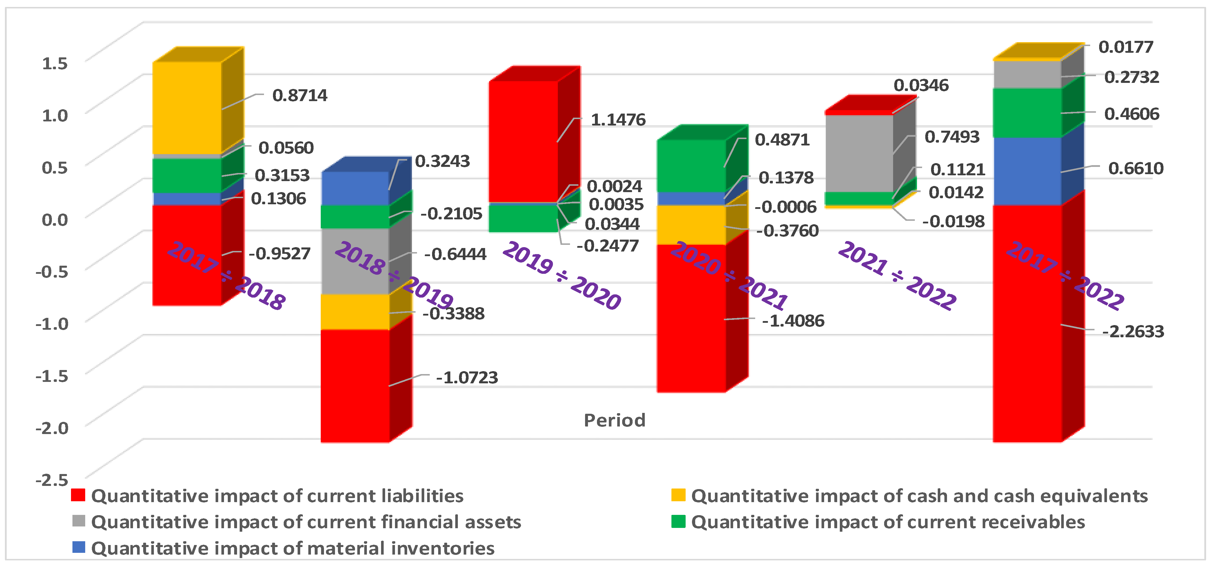
| Quantitative impact of material inventories (ΔTLR(In)) | 0.1306 | 0.3243 | 0.0344 | 0.1378 | 0.0142 | 0.6610 |
| Relative influence of material inventories (%TLR(MI) = ΔTLR(MI) * 100/TLRt−1), % | 1.81% | 4.25% | 0.61% | 2.08% | 0.26% | 9.17% |
| Quantitative impact of current receivables (ΔTLR(CR)) | 0.3153 | −0.2105 | −0.2477 | 0.4871 | 0.1121 | 0.4606 |
| Relative impact of current receivables (%TLR(CR) = ΔTLR(CR) * 100/TLRt−1), % | 4.38% | −2.76% | −4.36% | 7.35% | 2.05% | 6.39% |
| Quantitative impact of current financial assets (ΔTLR(CFA)) | 0.0560 | −0.6444 | 0.0035 | −0.0006 | 0.7493 | 0.2732 |
| Relative influence of current financial assets (%TLR(CFA) = ΔTLR(CFA) * 100/TLRt−1), % | 0.78% | −8.45% | 0.06% | −0.01% | 13.71% | 3.79% |
| Quantitative impact of cash and cash equivalents (ΔTLR(CCE)) | 0.8714 | −0.3388 | 0.0024 | −0.3760 | −0.0198 | 0.0177 |
| Relative influence of cash and cash equivalents (%TLR(CCE) = ΔTLR(CCE) * 100/TRLt−1), % | 12.09% | −4.44% | 0.04% | −5.68% | −0.36% | 0.25% |
| Quantitative impact of current liabilities (ΔTLR(CL)) | −0.9527 | −1.0723 | 1.1476 | −1.4086 | 0.0346 | −2.2633 |
| Relative impact of current liabilities (%TLR(CL) = ΔTLR(CL) * 100/TLRt−1), % | 13.22% | 14.06% | −20.19% | 21.27% | −0.63% | 31.41% |
| Complex influence ΔTLR = ΔTLR(MI) + ΔTLR(CR) +ΔTLR(CFA) + ΔTLR(CCE) + ΔTLR(CL) | 0.4207 | −1.9417 | 0.9402 | −1.1603 | 0.8904 | −0.8507 |
| Cumulative relative influence %TLR = %TLR(MI) + %TLR(CR) + %TLR(CFA) + %TLR(CCE) + %TLR(CL), % | 5.84% | −25.46% | 16.54% | −17.52% | 16.30% | −11.81% |
| Verification: ΔTLR = ΔTLR(MI) + ΔTLR(CR) + ΔTLR(CFA) + ΔTLR(CCE) + ΔTLR(CL) | False | True | True | True | False | True |
| Value of the absolute error, STLR, BGN/BGN | 0.0000000 | 0.0000000 | 0.0000000 | 0.0000000 | 0.0000000 | 0.0000000 |
| Verification: %TLR = %TLR(MI) + %TLR(CR) + %TLR(CFA) + %TLR(CCE) + %TLR(CL) | False | False | False | False | False | False |
| Value of the relative error, δTLR, % | 0.00000% | 0.00000% | 0.00000% | 0.00000% | 0.00000% | 0.00000% |
| Input Data | ||||||
|---|---|---|---|---|---|---|
| Indicator | Period | |||||
| 2017 | 2018 | 2019 | 2020 | 2021 | 2022 | |
| Value of Material Inventories, (MI), BGN’000 | 10,392 | 10,728 | 12,058 | 10,251 | 10,361 | 11,565 |
| Value of Current Receivables, (CR), BGN’000 | 6926 | 5264 | 3195 | 4009 | 4578 | 4989 |
| Value of Current Financial Assets, (CFA), BGN’000 | 0 | 0 | 0 | 0 | 0 | 0 |
| Value of Cash and Cash Equivalents, (CCE), BGN’000 | 783 | 1080 | 1841 | 3497 | 3330 | 2517 |
| Value of current liabilities, (CL), BGN’000 | 1531 | 1780 | 1481 | 1345 | 1920 | 2239 |
| Total Liquidity Ratio, (TLR) | 11.8230 | 9.5910 | 11.5422 | 13.2022 | 9.5151 | 8.5176 |
| Results obtained | ||||||
| Indicator | Analyzed period | |||||
| 2017–2018 | 2018–2019 | 2019–2020 | 2020–2021 | 2021–2022 | 2017–2022 | |
| 1 | 2 | 3 | 4 | 5 | 0–5 | |
| Absolute change in material inventories, (ΔMI = MIt − MIt−1), BGN’000 | 336 | 1330 | −1807 | 110 | 1204 | 1173 |
| Relative change in material inventories, (%MI = ΔMI * 100/MIt−1), % | 3.23% | 12.40% | −14.99% | 1.07% | 11.62% | 11.29% |
| Absolute change in current receivables, (ΔCR = CRt − CRt−1), BGN’000 | −1662 | −2069 | 814 | 569 | 411 | −1937 |
| Relative change in current receivables, (%CR = ΔCR * 100/CRt−1), % | −24.00% | −39.30% | 25.48% | 14.19% | 8.98% | −27.97% |
| Absolute change in current financial assets, (ΔCF = CFt − CFt−1), BGN’000 | 0 | 0 | 0 | 0 | 0 | 0 |
| Relative change in current financial assets, (%CF = ΔCF * 100/CFt−1), % | 0.00% | 0.00% | 0.00% | 0.00% | 0.00% | 0.00% |
| Absolute change in cash and cash equivalents, (ΔCCE = CCEt − CCEt−1), BGN’000 | 297 | 761 | 1656 | −167 | −813 | 1734 |
| Relative change in cash and cash equivalents, (%CF = ΔCF * 100/CFt − 1), % | 37.93% | 70.46% | 89.95% | −4.78% | −24.41% | 221.46% |
| Absolute change in current liabilities, (ΔCL = CLt − CLt−1), BGN’000 | 249 | −299 | −136 | 575 | 319 | 708 |
| Relative change in current liabilities, (%CL = ΔCL * 100/CLt−1), % | 16.26% | −16.80% | −9.18% | 42.75% | 16.61% | 46.24% |
| Absolute change in total liquidity ratio, (ΔTL = TLt − TLt−1) | −2.2320 | 1.9512 | 1.6600 | −3.6871 | −0.9975 | −3.3053 |
| Relative change in total liquidity ratio, (%TL = ΔTL * 100/TLt−1), % | −18.88% | 20.34% | 14.38% | −27.93% | −10.48% | −27.96% |
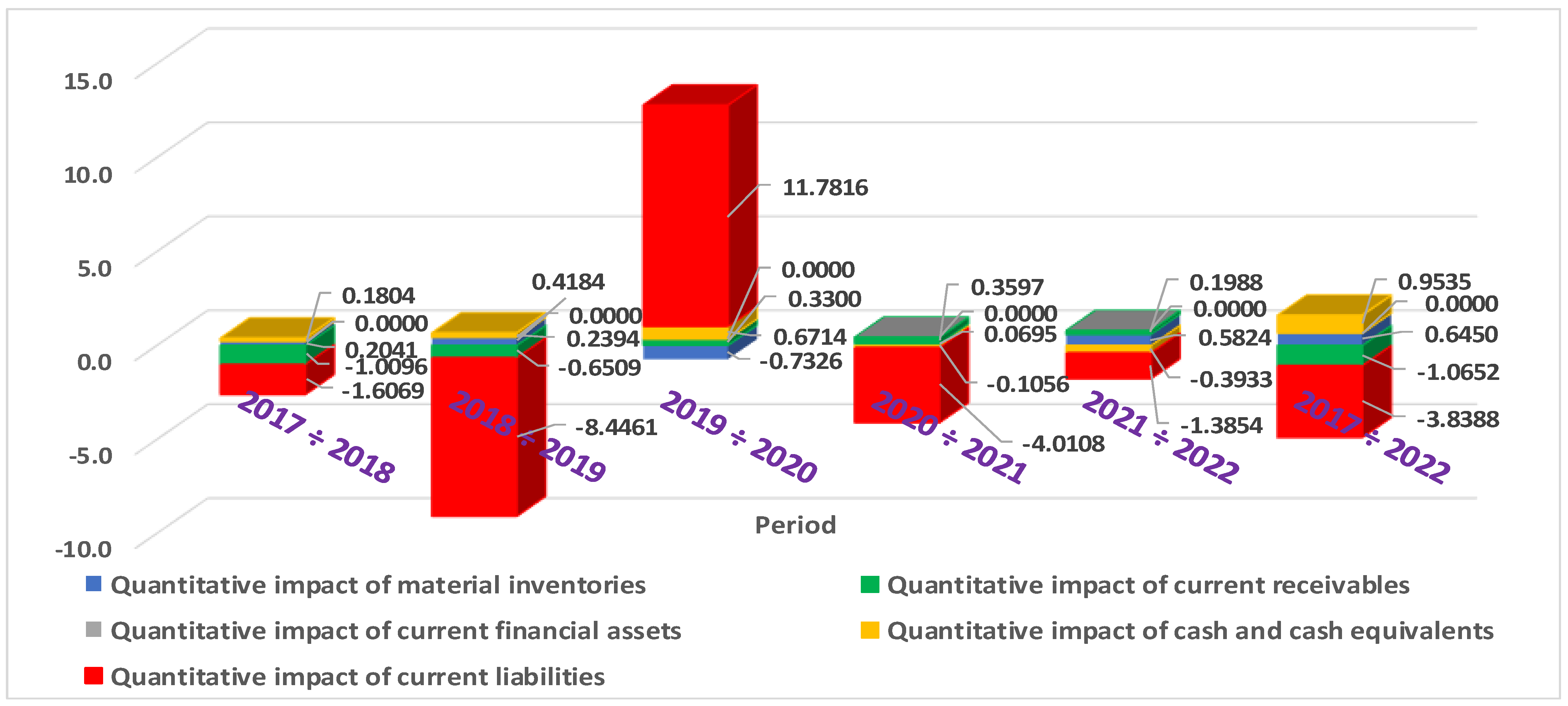
| Quantitative impact of material inventories, (ΔTLR(In)) | 0.2041 | 0.8226 | −1.2818 | 0.0695 | 0.5824 | 0.6450 |
| Relative influence of material inventories, (%TLR(MI) = ΔTLR(MI) * 100/TLRt−1), % | 1.73% | 8.58% | −11.11% | 0.53% | 6.12% | 5.46% |
| Quantitative impact of current receivables, (ΔTLR(CR)) | −1.0096 | −1.2797 | 0.5774 | 0.3597 | 0.1988 | −1.0652 |
| Relative impact of current receivables, (%TLR(CR) = ΔTLR(CR) * 100/TLRt−1), % | −8.54% | −13.34% | 5.00% | 2.72% | 2.09% | −9.01% |
| Quantitative impact of current financial assets (ΔTLR(CFA)) | 0.0000 | 0.0000 | 0.0000 | 0.0000 | 0.0000 | 0.0000 |
| Relative influence of current financial assets, (%TLR(CFA) = ΔTLR(CFA) * 100/TLRt−1), % | 0.00% | 0.00% | 0.00% | 0.00% | 0.00% | 0.00% |
| Quantitative impact of cash and cash equivalents, (ΔTLR(CCE)) | 0.1804 | 0.4707 | 1.1747 | −0.1056 | −0.3933 | 0.9535 |
| Relative influence of cash and cash equivalents, (%TLR(CCE) = ΔTLR(CCE) * 100/TRLt−1), % | 1.53% | 4.91% | 10.18% | −0.80% | −4.13% | 8.06% |
| Quantitative impact of current liabilities, (ΔTLR(CL)) | −1.6069 | 1.9376 | 1.1897 | −4.0108 | −1.3854 | −3.8388 |
| Relative impact of current liabilities, (%TLR(CL) = ΔTLR(CL) * 100/TLRt−1), % | 13.59% | −20.20% | −10.31% | 30.38% | 14.56% | 32.47% |
| Complex influence, ΔTLR = ΔTLR(MI) + ΔTLR(CR) + ΔTLR(CFA) + ΔTLR(CCE) + ΔTLR(CL) | −2.2320 | 1.9512 | 1.6600 | −3.6871 | −0.9975 | −3.3053 |
| Cumulative relative influence, %TLR = %TLR(MI) + %TLR(CR) + %TLR(CFA) + %TLR(CCE) + %TLR(CL), % | −18.88% | 20.34% | 14.38% | −27.93% | −10.48% | −27.96% |
| Verification: ΔTLR = = ΔTLR(MI) + ΔTLR(CR) + ΔTLR(CFA) + ΔTLR(CCE) + ΔTLR(CL) | True | True | True | True | True | True |
| Value of the absolute error, STLR, BGN/BGN | 0.0000000 | 0.0000000 | 0.0000000 | 0.0000000 | 0.0000000 | 0.0000000 |
| Verification: %TLR = = %TLR(MI) + %TLR(CR) + %TLR(CFA) + %TLR(CCE) + %TLR(CL) | False | False | False | False | False | False |
| Value of the relative error, δTLR, % | 0.00000% | 0.00000% | 0.00000% | 0.00000% | 0.00000% | 0.00000% |
Disclaimer/Publisher’s Note: The statements, opinions and data contained in all publications are solely those of the individual author(s) and contributor(s) and not of MDPI and/or the editor(s). MDPI and/or the editor(s) disclaim responsibility for any injury to people or property resulting from any ideas, methods, instructions or products referred to in the content. |
© 2024 by the authors. Licensee MDPI, Basel, Switzerland. This article is an open access article distributed under the terms and conditions of the Creative Commons Attribution (CC BY) license (https://creativecommons.org/licenses/by/4.0/).
Share and Cite
Mitev, V.; Hinov, N. An Innovative Method for Deterministic Multifactor Analysis Based on Chain Substitution Averaging. Mathematics 2024, 12, 2215. https://doi.org/10.3390/math12142215
Mitev V, Hinov N. An Innovative Method for Deterministic Multifactor Analysis Based on Chain Substitution Averaging. Mathematics. 2024; 12(14):2215. https://doi.org/10.3390/math12142215
Chicago/Turabian StyleMitev, Veselin, and Nikolay Hinov. 2024. "An Innovative Method for Deterministic Multifactor Analysis Based on Chain Substitution Averaging" Mathematics 12, no. 14: 2215. https://doi.org/10.3390/math12142215
APA StyleMitev, V., & Hinov, N. (2024). An Innovative Method for Deterministic Multifactor Analysis Based on Chain Substitution Averaging. Mathematics, 12(14), 2215. https://doi.org/10.3390/math12142215