Abstract
There is uncertainty in the results of any mathematical model due to different reasons. It is important to estimate this uncertainty. Sensitivity analysis is commonly used to estimate how the changes in the input parameters affect the solutions of the model. In this paper, we discuss different ways of performing local and global sensitivity analyses and apply them to two models: an epidemic model and a new myocardial infarction model, both based on ordinary differential equations. The first model is a simple model used to explain the ideas, while the second one shows how to apply them to a model with more state variables and parameters. We find that if the parameters are not accurately known, local sensitivity analysis can be misleading and that global sensitivity methods that sample the whole parameter space, varying all the values of the parameters at the same time, are the most reliable. We also show how the sensitivity analysis results can be used to determine the uncertainty in the results of the model. We present numerical simulations.
MSC:
65L05
1. Introduction
Mathematical models take inputs, such as the parameters and the initial conditions, and transform them into outputs. There is uncertainty in the outputs due to simplifications, incorrect hypotheses, errors in measuring the data, missing data, variability in the populations, and, in general, incomplete knowledge. In order for the results of the model to be reliable, it is important to estimate the size of the uncertainty. A related but different issue is determining how variations in the model parameters affect the solutions. Sensitivity analysis deals with uncertainty in the parameters of the model. Determining the parameter values with precision is a difficult task due to large variations and heterogeneities in populations and other uncertainties associated with their measurement. In many cases, they may also have to be estimated indirectly. Therefore, it is important to establish how sensitive the model solutions are to changes in the values of parameters and to establish the relative importance of different parameters on the output of the model. Some references on sensitivity analysis include [1,2,3,4] and the comparative papers [5,6,7]. These days, many papers dealing with mathematical models of biological, economic, and many other areas include a section on sensitivity analysis. The perspective paper [8] reviews the status quo of sensitivity analysis and makes a case for its use for advancing mechanistic and data-driven models. Some examples of applications of sensitivity analysis to models with very high complexity include [9,10]. As the models become more complex, the uncertainty in their solutions increases, and so does the number of related papers, for example, [11,12,13,14]. One method for determining the uncertainty in the results of a model based on ordinary differential equations (ODEs) is to use random ordinary differential equations (RODEs). The uncertainty involving such phenomena appears through the model inputs (parameters and initial/boundary conditions), which are regarded as random variables and stochastic processes rather than constants [15]. Generalized polynomial chaos can be used to numerically approximate the solutions of RODEs by estimating their mean and standard deviation [16,17,18]. But there are other methods for RODEs [19]. A second method considers that some or all of the parameters have a constant term plus a white noise term. Then, stochastic differential equations (SDEs) are obtained [20,21,22] or the white noise may be added as additive or multiplicative noise [23,24,25,26]. Alternative methods can be found in [27,28].
A simple epidemic model consists of three populations: susceptibles (S), who can become infectives (I) after contact with an infective, then recover (R) with complete temporal immunity, and finally return to the susceptible class. This is the SIRS model [29,30]. We will use this relatively simple epidemic model to illustrate the differences in using different methods of sensitivity analysis and uncertainty quantification.
Our main model is a new heart infarction model. Preliminary work on this model and its sensitivity indices can be found in [31]. Heart-related diseases are the leading cause of death worldwide. The World Health Organization keeps track of deaths due to heart infarction, and according to their website, there are more than seven million deaths every year [32]. Unhealthy diets and stress are among the causes of the buildup of plaque within the walls of the arteries. This buildup obstructs the flow of blood, causing atherosclerosis. The amount of blood to the heart tissues is then reduced, and this decrease is the reason the heart cells do not receive enough oxygen. Coronary artery disease, left untreated in many cases, will lead to myocardial infarction (MI), also known as a heart attack. This happens when a reduced flow of blood (ischemia) and reduced oxygen (hypoxia) in a region of the heart cause the death of cardiac muscle cells. Sometimes, a myocardial infarction will occur when a portion of the plaque moves through the arteries and blocks one of the smaller vessels. Some references include [33,34,35,36]. The survival rates after suffering a heart infarction have improved in recent years, but the loss of cardiomyocytes, which reduces the function of the heart, is a major problem for affected individuals. Since there are no stem cells in the heart to replace the dead cardiomyocytes, there is very active research to find alternative sources of cardiomyocyte progenitors, but there are still no clear answers [37].
The rest of this paper is organized as follows. In Section 2, we present the SIRS and heart infarction mathematical models, the different sensitivity analysis methods, and the formulations for the stochastic differential equations. Section 3 discusses the numerical results and simulations. Section 4 presents the discussion and conclusions.
2. Materials and Methods
2.1. Mathematical Models
We consider two main models: an SIRS epidemic model that is simple, making the differences in the results of using different methods easy to observe, and the new MI model. We consider two variations of this model.
2.1.1. SIRS Model
For short-duration epidemics with low mortality rates, such as influenza, a simple model is the SIRS model with no demographics [30]. It consists of three population classes: susceptibles (), infectives or infected (), and recovered (). A susceptible individual has a given probability of turning into an infective after contact with an infective. is the average number of contacts per unit time for a successful infection, so is the average number of contacts with infectives per unit time of one susceptible, and is the number of new infectives per unit time [38]. An infective recovers with a rate . A recovered individual loses immunity at a rate and converts again into a susceptible. With no demographics, the total population is constant, . is usually called the infection or transmission coefficient. All parameters are positive, and the populations are non-negative. For well-mixed homogeneous populations, the infection process has no spatial dependence, and the model is given by a system of ordinary differential equations [29,30]
Since the total population is constant, the model can be simplified: eliminate the last equation and the state R using . The new system consisting of only two equations is
The SIRS model, given by either (1) or (2), has two equilibrium states: the disease-free equilibrium DFE, ; and an endemic equilibrium, . The endemic equilibrium makes biological sense only for . For the SIRS model, the basic reproduction (or reproductive) number is [30,39].
2.1.2. Heart Infarction Model
The types of cells present in the heart and the many signaling and chemical factors involved in the different processes are well known. Next, we summarize the results given in, for example, [40,41,42,43], and stated in [31]:
There are many different types of cells that form the heart: cardiomyocytes (or just cardiocytes or myocytes), which comprise 20–35% of heart cells; endothelial cells, which are the most abundant (60%) among non-cardiomyocytes and are involved in the formation of new blood vessels; fibroblasts, which are also very abundant and synthesize the cardiac extracellular matrix; pericytes, which are smooth muscle-like cells; and a variety of immune cells. Following any injury, these cells are rapidly recruited in large numbers to the heart [40]. There is a large variety of immune cells, the most abundant being neutrophils, monocytes, and macrophages, including both pro-inflammatory M1 and anti-inflammatory M2. Less common are dendritic cells, lymphocytes, and mast cells [41]. Many papers explore empirical research on the participation of the immune cells in MI. A good review is given in [44]. Neutrophils and macrophages ingest dead cardiomyocytes and also interact by producing and accepting chemical substances such as cytokines, chemokines, and growth factors. Some of these factors are pro-inflammatory, like , tumor necrosis factor (TNF), , and , while others are anti-inflammatory, like , TGF-, and TNF- [42]. After a myocardial infarction, the heart starts healing itself. The healing process has four distinct phases, but there is some overlap [43]:
- Necrotic phase: heart cells die rapidly (starts soon after after MI).
- Acute inflammatory phase: the immune system responds and starts eliminating dead cells (1–7 days).
- Sub-acute granulation phase: myofibroblasts proliferate to form granulation tissue to help stabilize the heart (1–3 weeks).
- Chronic scar phase: myofibroblast proliferation continues, leading to the generation of the final scar tissue (1 month).
In this paper, we model the first two phases: the death of cardiomyocytes due to lack of oxygen, and how the immune system eliminates the dead cells from the heart. There is a great body of literature on experimental work on the immune system after MI, for example, [43,45,46,47,48]. There are also many papers studying the effect of molecular mediators on various cells, for example, [42,49,50]. The number of mathematical models is much smaller. Some existing mathematical models include the model given in [51], which includes monocytes, macrophages M1 and M2, , and . The model presented in [52] includes macrophages, fibroblasts, TGF-, MMP-9, and collagen. The authors of [53] model neutrophils, apoptotic neutrophils, macrophages, a pro-inflammatory mediator, and an anti-inflammatory mediator. There is a recent review of models of the immune system in [54].
We develop two related mathematical models of MI. The first one models the second phase: a percentage of cardiomyocytes have died due to lack of oxygen, and the immune system is eliminating the dead cells, including dead neutrophils. The second model also includes the first phase, which involves the death of cardiomyocytes. The second model is a minor extension of the first since the interactions between the immune system cells and dead cardiomyocytes are not affected. The first phase is included since we want to study the effect of the time between the MI and the restoration of oxygen on the results of an MI. Since there is no spatial dependence, both MI models are described using ordinary differential equations.
The models were developed using the following hypotheses introduced in [31]: We consider a small part of the heart that is damaged by the MI. Therefore, we assume that the distribution of all the involved cells is uniform and homogeneous. The involved cells communicate through chemical factors, and for simplicity, we assume that the amount of each factor is proportional to the number of cells that produce it. After the myocardial infarction, cardiomyocytes die until the oxygen is restored. Neutrophils are the first immune system cells involved. They phagocytosize the dead cardiomyocytes. After the arrival of neutrophils, monocytes circulating in the blood migrate to the site of the infarction, where they differentiate into macrophages of types M1 (pro-inflammatory) and M2 (anti-inflammatory) and gradually replace the short-lived neutrophils. M1 macrophages continue phagocytosizing dead cardiomyocytes and also dead neutrophils. The number of dead cells controls the rate of conversion of monocytes to M1 macrophages. Macrophage conversion from M1 to M2 is still not well understood but involves several molecular and cellular factors and macrophage phagocytosis. M2 macrophages inhibit M1 macrophages, so they do not destroy healthy cells. After all the dead cells (cardiomyocytes and neutrophils) have been eliminated, the remaining neutrophils and M1 macrophages also leave the system. Among the many papers that propose and experimentally validate these hypotheses are [41,42,43,51,52,54,55].
The first MI model, Model 1, deals with the second phase of the MI process. The mathematical model consists of six ordinary nonlinear differential equations for the state variables: dead cardiomyocytes, ; neutrophils, N; dead neutrophils, ; monocytes, M; M1 macrophages, , and M2 macrophages, . The interactions are governed by the above hypotheses. The system of equations that describes the evolution in time of these six populations is given by Equation (3). The model involves sixteen parameters. All parameter values are assumed to be positive. Some are obtained from the literature, while others need to be established through reasonable estimation. More details are given in Section 3.
Theorem 1.
The model (3) has only one biologically realistic equilibrium point: , , , , , and .
Proof.
Since all populations have to be non-negative to make biological sense, all parameters are positive. The right-hand side of Equation (3a) equals zero: , gives , or . Case I: . Using Equation (3b), the only non-negative value for N is . Then, from the steady state for Equation (3c), . For , the steady state of Equation (3d) gives . implies from the steady state of Equation (3e) that , and implies from Equation (3f) that . Case II: , and . From the steady state of Equation (3b), , which brings us back to Case I. So, the only steady solution is the zero solution. □
Theorem 2.
For non-negative initial conditions, System (3) has non-negative solutions.
Proof.
According to the fundamental existence-uniqueness theorem for ordinary differential equations, no positive solution can intersect the zero (steady) solution. □
Theorem 3.
The solutions of System (3) are bounded above.
Proof.
From Equation (3a), . From Equation (3b),
and integrating the inequality gives
where . So, N is bounded above. From Equation (3c),
where is an upper bound for N, so by solving for , we have that it is bounded above. Similarly, from (3d)–(3f), we have
and integrating we have that , and are bounded above. Here, and are the maximum values of M and , respectively. □
To study the local stability of this equilibrium point, we linearize System (3). The Jacobian matrix, ordering the equations as in (3) and the variables as , and , is
and the Jacobian matrix evaluated at is
Its eigenvalues are .
Theorem 4.
The steady solution is stable.
Proof.
Five of the eigenvalues are negative, and the sixth one is zero. Therefore, determining the stability usually requires the use of the Center Manifold Theorem [56]. In this case, the linearized system is not decoupled into stable and center components, and the change in variables to obtain a diagonal system produces a complicated matrix. However, as , from Equation (3a), tends to be a constant, which has to be zero since this is the only steady state. Looking at this limit from (3b), we see that N also tends to zero, and similarly for the other populations. Therefore, the steady state is asymptotically stable. □
The analysis of the model shows that the zero solution is the only biologically realistic equilibrium point. The zero solution is when the number of all involved cells is zero. This solution is asymptotically stable. There are sixteen parameters in the model. Empirical values of the parameters are few and the reported values have large variations. The decay rates are the best-known of all the parameters. The second model, Model 2, also includes the first phase and adds an equation for live cardiomyocytes that die due to lack of oxygen. Since Model 1 starts with the restoration of oxygen, it does not need to include live cardiomyocytes.
In Model 2, we consider the cardiac infarction to start when the flow of blood and oxygen is interrupted. Cardiomyocytes start to die and stop dying when the flow of blood is restored. After that time, the processes involving dead cardiomyocytes and the immune system are the same as those in Model 1. Model 2 has an extra population, C, representing healthy cardiomyocytes. The system of equations describing the model is
where Heaviside(·) is the Heaviside function and is the time in days from the restriction of the blood flow to when the flow and oxygen are restored.
For , there is no steady solution since C is decaying. For , there is a steady solution, with C and constant and the other populations zero. This is shown similarly to how it was done for Model 1.
Since from Equation (4a), C decays exponentially until oxygen is restored and is constant after that, C is bounded and non-negative. C only affects Equation (4b) such that the growth rate of is bounded by for , allowing to grow at most linearly, and by , ensuring is still bounded above. So, the same procedure used for Model 1 can be used to show that all other populations are bounded above. For , Equation (4b) has an extra positive term on the right-hand side, so if was non-negative in Model 1, it will still be non-negative in Model 2, as will the other populations.
For , there is no steady solution. For , Equation (4a) has a right-hand side of zero, decoupling it from the other equations. Since Equation (4a) is linear, C is stable, and so is the complete System (4), following the results of Model 1.
2.2. Sensitivity Analysis
Mathematical models have a number of parameters. Most of these parameters are not accurately known since determining their values is difficult due to many reasons: large variations in populations, measurement errors, missing data, and other uncertainties. Many parameters also need to be estimated indirectly. Therefore, it is important to determine how the model outputs change as the parameter values change. Ideally, a change in a parameter should produce a change in the solutions of the same order of magnitude. Large sensitivity indices indicate high uncertainty in the output and potential errors. Very small sensitivity indices with respect to a given parameter indicate that the model may be simplified. Sensitivity analysis can be local or global. Local sensitivity analysis determines the sensitivity of the model to changes in parameter values within a localized region around a given set of parameter values. Changes are made one parameter at a time, so local sensitivity analysis assumes there is no interaction between parameters [57,58,59,60]. Global sensitivity analysis (GSA) estimates sensitivity across the whole range of possible parameter values and usually considers that there may be interactions between the effects of the parameters [61,62]. Local sensitivity analysis is easy to implement and fast to solve. But if the parameters are not accurately known or if they are not independent, the results may not be reliable [63]. Global sensitivity analysis explores the parameter space and is more reliable. There are different global sensitivity methods: Sobol’s method [62,64,65], the Fourier amplitude sensitivity test (FAST) method [62,66], the extended Fourier amplitude sensitivity test (EFAST) method [67,68], the Morris method [3,69], the partial rank correlation coefficient (PRCC) method [70,71], and others. Some papers comparing local and global sensitivity analysis include [2,64,72,73].
The outputs of the model are functions of time, and so are the sensitivity indices. Also, there is a sensitivity index for each model state variable with respect to each parameter. Therefore, there is a large amount of sensitivity data. Possible ways of eliminating the time dependence include considering the indices only at steady solutions, at a few selected times, or at their averages across the simulation time. Other ways of reducing the amount of information include considering only the indices for one relevant variable, such as the number of infectives or the number of dead cardiomyocytes, and considering only the average, maximum, and minimum values of the indices of the unknown variables.
Next, we calculate the local sensitivity indices inexpensively using an augmented system of ordinary differential equations. The indices are calculated using several global sensitivity analysis methods [1,74,75].
To implement local sensitivity analysis, consider
where y is the vector of state variables and p is the vector of the parameters of the model. The local sensitivity index with respect to the parameter is defined as
and satisfies the forward sensitivity equations
obtained by applying the chain rule to the system of ordinary differential Equation (5) [76].
Local sensitivity analysis indices are fast to calculate and the procedure is straightforward. But local sensitivity analysis methods only evaluate the indices at one point in the parameter space and do not take into account their variability. Furthermore, local methods approximate the partial derivatives by changing the values of the parameters one at a time. Therefore, they implicitly assume no interaction between parameters. Also, the sensitivities are a matrix function of time (6). To reduce the amount of information and to make it easier to determine the parameters with the greatest sensitivities, usually only the average sensitivity indices over the time interval of interest are considered.
Local sensitivity indices may be normalized. This helps deal with size differences in the values of the variables and parameters. The normalized sensitivity indices are defined as where is the local sensitivity index, parameter is the value of the corresponding parameter, and variable is the value of the state variable. But normalization can create large errors if the variable values are close to zero, as in the heart infarction model. Some packages for computing local sensitivity indices include CVODES [76]; SciMLSensitivity.jl in Julia, which also calculates exact derivatives [77]; odeSensitivity in Matlab [78], and any ODE numerical solver.
Global sensitivity analysis methods consider that the values of the parameters have a range of interest. The methods are expensive since they explore the entire parameter space. The choice of sampling method is an important decision. A common alternative is to use the Latin hypercube sampling method to generate random points at which to evaluate the parameters [79]. Alternatively, a Monte Carlo method can be used to generate sampling points. The Latin hypercube method generates points that are more evenly distributed in the parameter space. Another sampling method is Sobol’s method [80,81]. Global sensitivity methods can be grouped into two types: regression-based methods with rank transformation, among which the PRCC method is probably the best known [82], and variance-based methods, among which Sobol’s method [62] and the FAST method [83] are good examples. Some general references for global sensitivity methods include [67,70]. The PRCC method is computationally cheaper compared to other global methods, but it can produce unreliable results if the state variables do not depend monotonically on the parameters. There are many software packages that implement global analysis, but most are designed for algebraic models. Two very good ones designed for ODEs are the SAFE Toolbox in Matlab [67,84] and GlobalSensitivity.jl in Julia [85]. We used both of them. Our choice was based on the programming languages, ease of use, and features. For example, the SAFE Toolbox runs in Matlab/Octave and also in R and Python. It also computes the convergence rates and explicitly gives the solution to the ODEs. The Julia program runs significantly faster.
2.3. Stochastic Differential Equations
Consider the simple ODE
Usually, the parameter is considered deterministic. However, due to measurement errors, variability in populations, lack of sufficient data, and other factors that introduce uncertainties, can be treated as a random variable, , where is its mean value and is a white noise process [20,22]. The differential form of Brownian motion is defined as . Then, the stochastic differential equation corresponding to the deterministic Equation (7) is
The general form of a stochastic differential equation is
where f is the deterministic part and g is the random part. is one of the possible values of the parameters, and is a time-dependent random variable (or stochastic process). Stochastic differential equations can be used in models where there is a need to include uncertainty and variability. Most models dealing with physical, biological, social, or economic processes fall into this category.
Most stochastic differential equations need to be solved numerically. Using Ito’s calculus, numerical methods for ODEs can be modified for solving SDEs [86,87,88]. Random differential equations can also estimate uncertainty in the outputs of mathematical models. Numerical approximations, such as polynomial chaos, are expensive and hard to program for models with many random parameters. But the calculations used in global sensitivity analysis can be applied, as we illustrate later.
3. Results
3.1. SIRS Epidemic Model
The deterministic SIRS model with no demographics and constant population N is given by Equation (2). Seasonal influenza is one of the epidemics that can be modeled using this model. The values of the parameters , and used are based on those given in [89] and by the CDC [90] for seasonal influenza, and they are given in Table 1.

Table 1.
This table has the parameter values used in the simulations.
The total population is scaled to 1000. and are known with good accuracy, but has significant variation depending on factors such as the concentration of the population (urban vs. rural), the types of social interactions, and more. The initial conditions are and .
3.1.1. Sensitivity Analysis
Sensitivity analysis studies how variations in the input parameters affect the outputs of the model. The SIRS model (1) is a good model for comparing different sensitivity analysis methods since there are only two variables and three parameters.
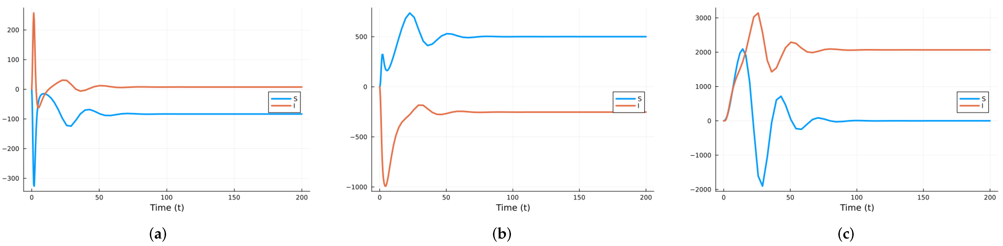
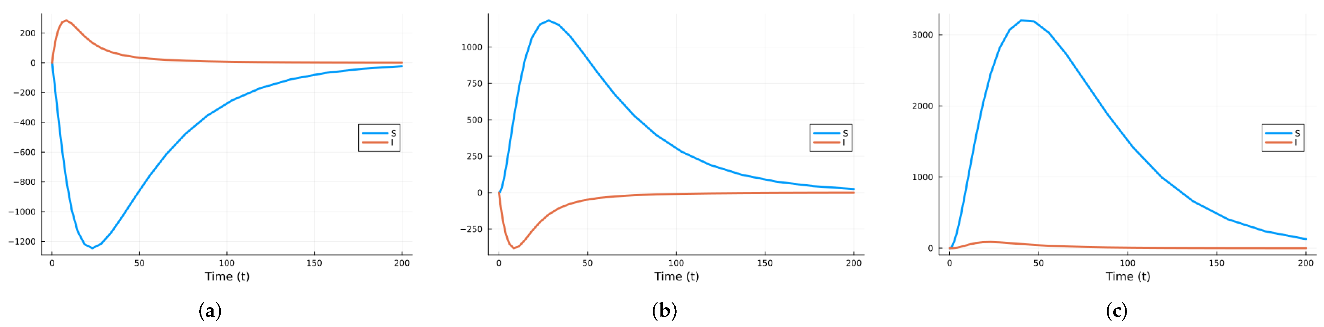
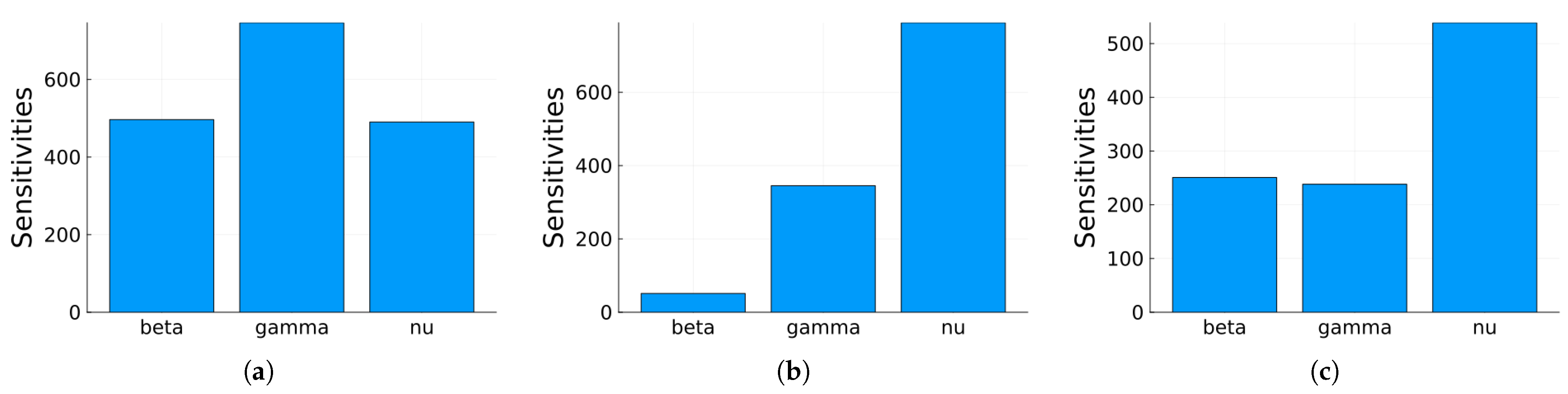
First, we calculate the local sensitivity indices for S and I with respect to the three parameters , and as functions of time. Since can vary the most, the process is repeated with two other values of . Next, for each state variable, we compute the time-averaged indices, followed by averaging across the two state variables. Figure 1 shows the time-varying indices for both S and I with respect to each parameter using the values in Table 1. Figure 2 and Figure 3 show the same results but for , corresponding to , and , corresponding to , respectively.
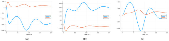
Figure 1.
SIRS local indices using the parameter values given in Table 1 (a) with respect to , (b) with respect to , (c) with respect to .
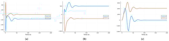
Figure 2.
SIRS local indices using the parameter values given in Table 1 for (a) with respect to , (b) with respect to , (c) with respect to .
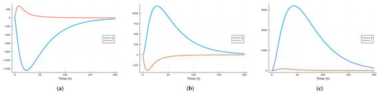
Figure 3.
SIRS local indices using the parameter values given in Table 1 for (a) with respect to , (b) with respect to , (c) with respect to .
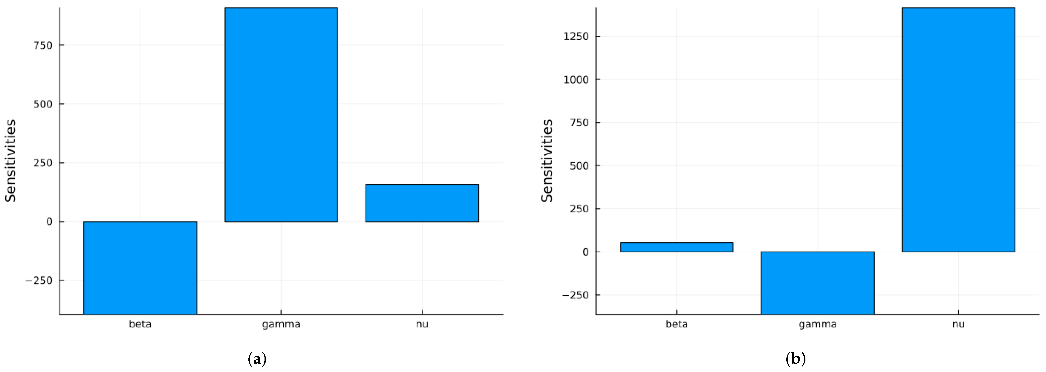
As can be seen in the figures, the curves for the sensitivity indices sometimes cross. So, looking at the indices at specific times can lead to misleading conclusions. It is better to take the mean over the time interval of interest. Figure 4 shows the mean indices for S with respect to the three parameters for , and . Figure 5 shows the mean indices for I with respect to the three parameters for , and . As can be seen, varying the value of can change the relative importance of the indices. So, unless all parameters are known with good accuracy, local sensitivity indices may give misleading results.

Figure 4.
SIRS time-averaged local indices for S using the parameter values given in Table 1 (a) for , (b) for , (c) for .
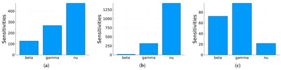
Figure 5.
SIRS time-averaged local indices for I using the parameter values given in Table 1 (a) for , (b) for , (c) for .
Figure 6 shows the average over the two state variables of the time-averaged indices with respect to the three parameters for , and . Now, it is easier to determine the order of importance of the indices. But this order still depends on the value of .

Figure 6.
SIRS mean for the two state variables of the time-averaged local indices using the parameter values given in Table 1 (a) for , (b) for , (c) for .
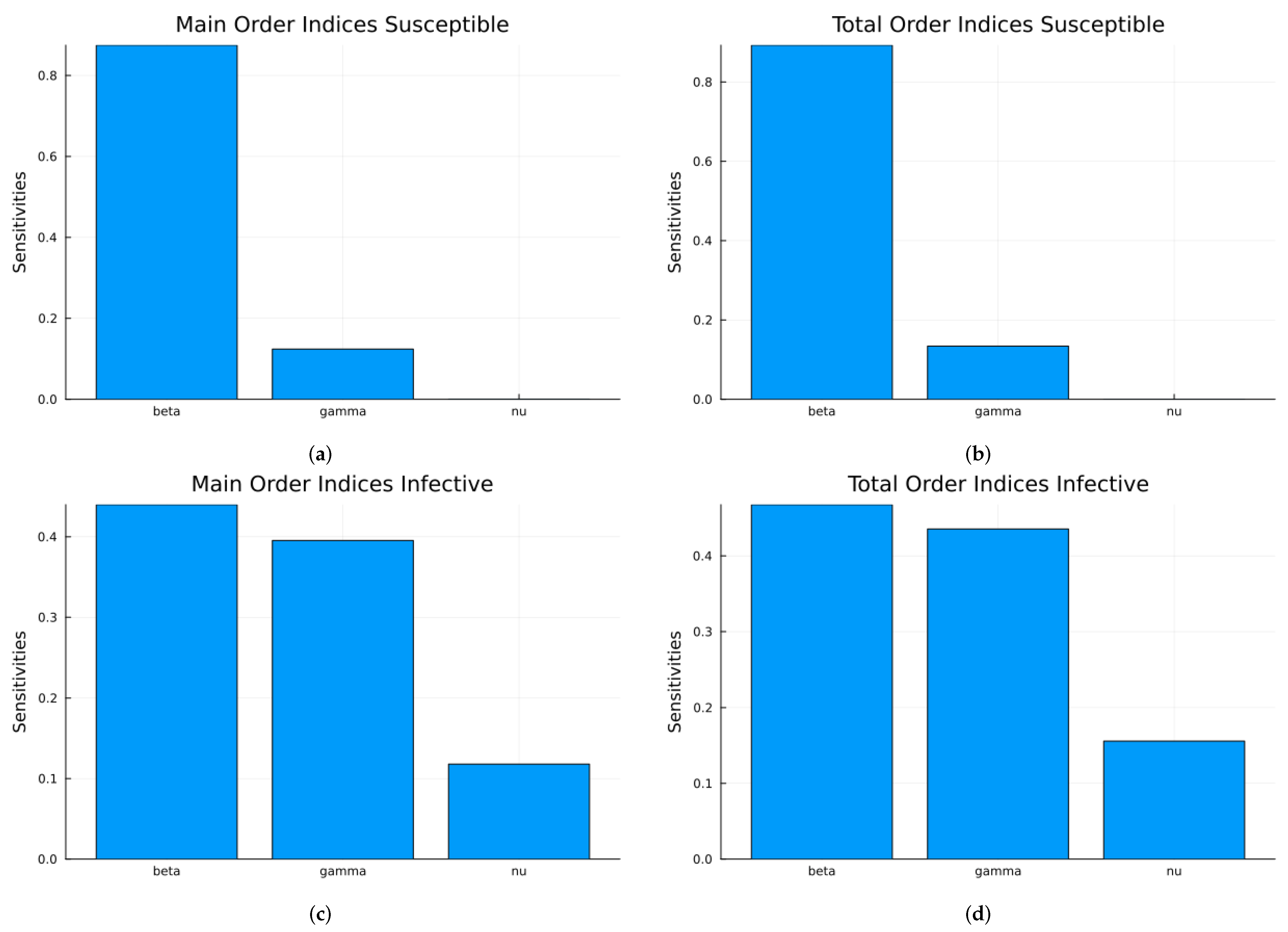
Next, we use two global sensitivity methods: the Morris method [69], which varies the parameters across their ranges one at a time, and Sobol’s method [62], which varies all parameters at the same time. Sobol’s method calculates the main indices, which represent the individual contributions of each parameter, and the total indices, which include interactions between parameters. The difference between these indices is an indicator of the strength of the interactions. Note that the Sobol method solves the ODE system for parameter values across their ranges. The three parameters are assumed to have uniform distributions: in the interval [0.2, 2.0], in the interval [0.2, 0.5], and in the interval [1/40, 1/15]. has a larger range since in real epidemics, it can vary more. Figure 7 shows the time-averaged indices for S and I with respect to the three parameters using the Morris method. Some software packages yield negative indices when increasing a parameter decreases the value of a state variable, while others keep the indices non-negative. If we are more interested in the infective population, then the index with respect to is the most important.

Figure 7.
SIRS global Morris indices using the parameter values given in Table 1: (a) Indices for S. (b) Indices for I.
Figure 8 shows the time-averaged indices for S and I with respect to the three parameters, calculated using Sobol’s method. The top graphs are the main and total indices for S, and the bottom graphs are the same indices for I. The most relevant indices are those with respect to . Since one-at-a-time sampling is much more limited compared to Latin hypercube sampling or Monte Carlo sampling, the results from Sobol’s method are more reliable.

Figure 8.
SIRS global Sobol indices using the parameter values given in Table 1: (a) Main indices for S. (b) Total indices for S. (c) Main indices for I. (d) Total indices for I.
3.1.2. Stochastic and Random Differential Equations
To estimate the uncertainty in the solutions of a mathematical model, the mean values and variance of the solutions can be used. One way to achieve this objective is to use SDEs. There are many different ways to construct a stochastic system. For the SIRS model, they are as follows:
The noise is considered environmental and is denoted as additive noise. An open question is the determination of the values of the amplitude: the s.
A second way is to consider that the noise depends on the size of the corresponding population
This noise is called multiplicative. There is also the issue of determining the amplitude of the noise.
A third way is to consider that the parameters have a deterministic part plus a random part given by a white noise term. This can be labor-intensive when dealing with many parameters. But we can use the information from sensitivity analysis and consider only parameters with the most relevant indices. For the SIRS model, these parameters are and , as given by Sobol’s method. The amplitude of the noise can be estimated based on empirical data for parameter variation.
For , centered at , we chose , and for , centered at , we chose .
A fourth way is to start with a discrete-time Markov chain and calculate the probabilities of a population staying in or exiting a given state. Under certain assumptions, a stochastic system of differential equations is obtained, which is not unique. For more details, see [27]:
where
For systems with many state variables and parameters, implementation is complicated.
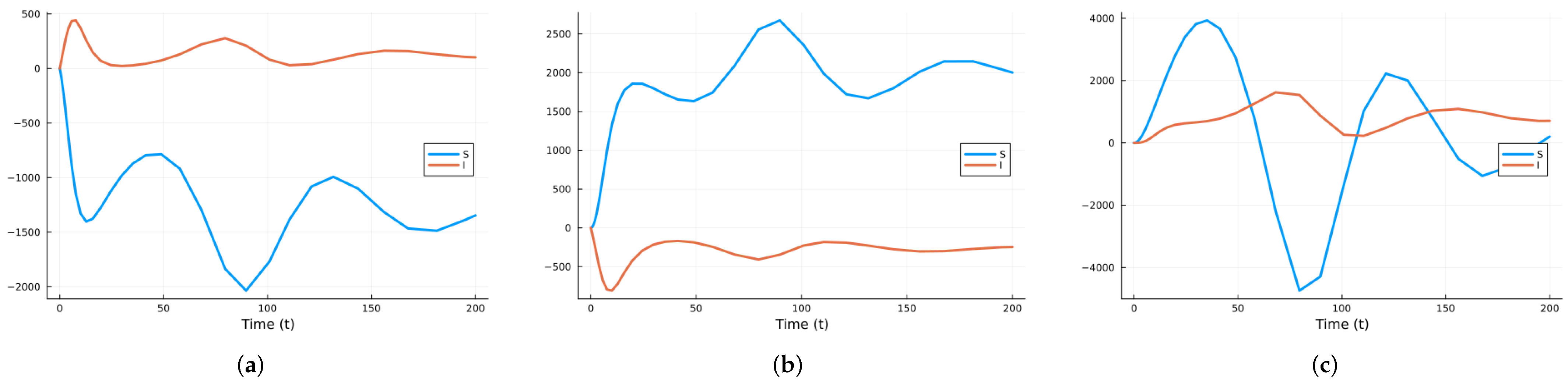
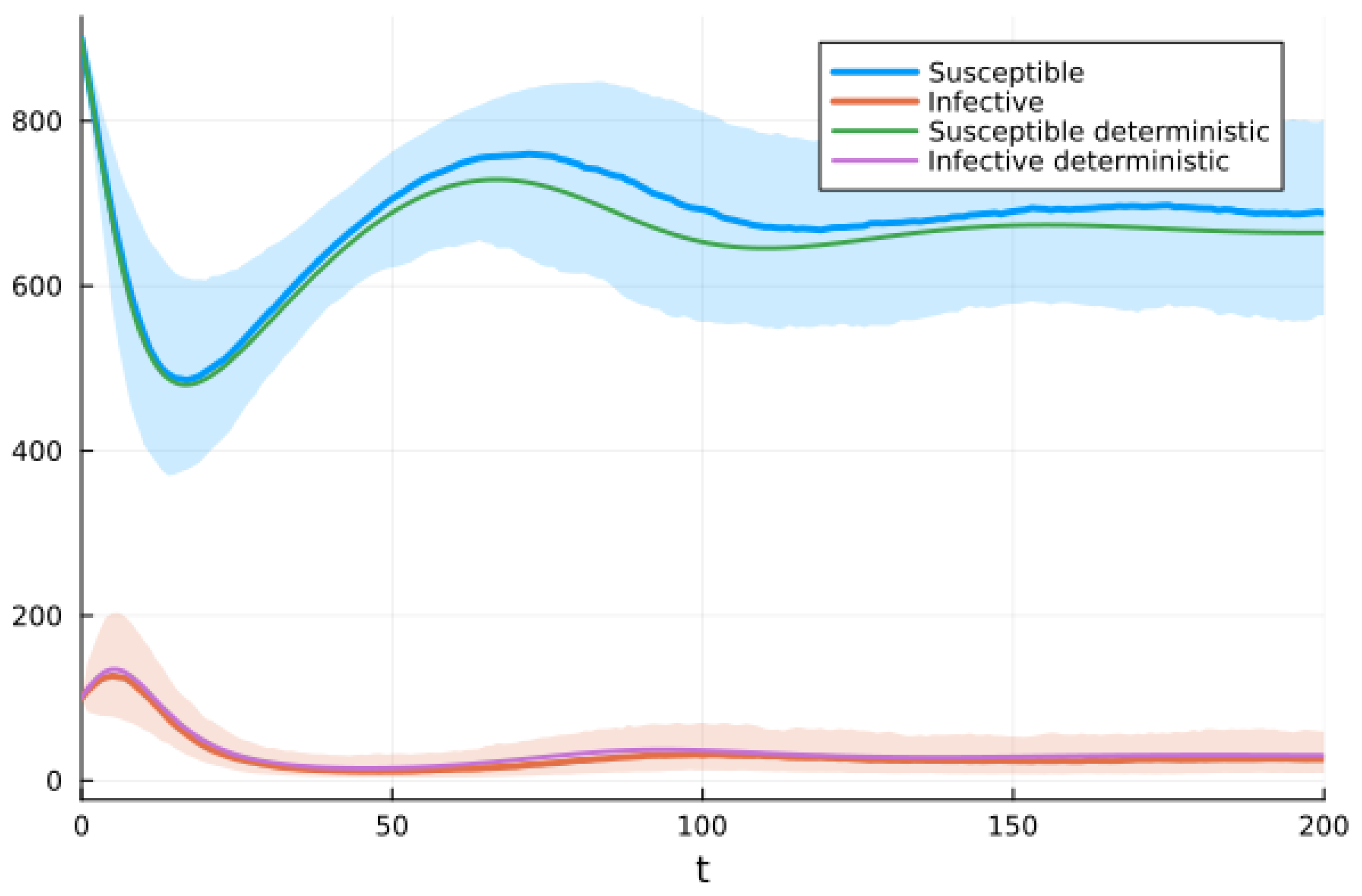
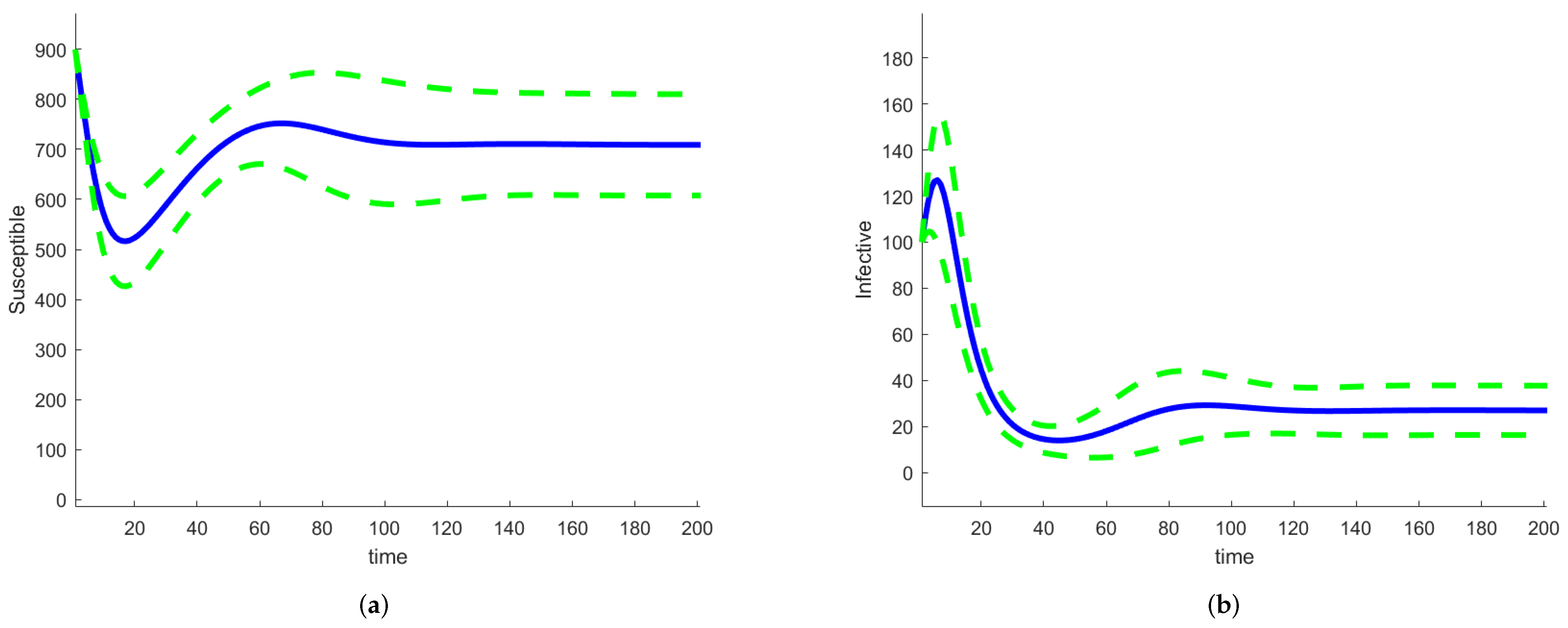
We chose the third option and used the Julia package DifferentialEquations.jl [91] to solve the system of SDEs using a method based on the Runge–Kutta method. Figure 9 shows graphs of the deterministic solution, the mean, and the mean plus/minus one standard deviation for the SDEs given by system (10). We performed 500 realizations and then another 500. Since the results were almost identical, we stopped the simulations. We realize that there is a possibility this was not enough.

Figure 9.
Solutions of SIRS deterministic system (2) and system of SDEs (10). For the SDEs, the solid line is the mean, and the shaded areas are the mean ± standard deviation.
If we use Sobol’s method to calculate the sensitivity indices, we already have the solution to the deterministic model with the parameters sampled across their ranges. This is also true for the FAST method and any other method that samples the complete parameter space. We solved the model equations by assuming that the parameters are random variables with a given distribution and by using a large number of sample points. These solutions can be used to estimate the means and standard deviations of the solutions of the random differential equations equations, thus providing an estimate of the uncertainties in the outputs of the model. We used the SAFE Toolbox [67] and the FAST method to evaluate the sensitivity indices. The SAFE Toolbox estimates the number of evaluations necessary for the calculation of the indices to converge. For this model, it was 5000. There is no need to estimate the amplitude of the random term; it depends on the parameter variation intervals. Figure 10 shows graphs of the mean values of S (left) and I (right), together with curves representing the mean ± standard deviation.
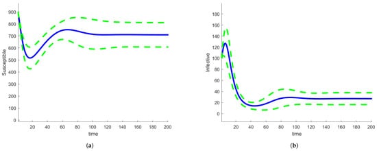
Figure 10.
SIRS random differential equation model mean and mean ± standard deviation (a) for S, (b) for I.
3.2. Heart Infarction Model
We now consider our main interest, which is the heart infarction model. Since during the first phase of myocardial infarction, only cardiomyocytes die, we conduct sensitivity analysis and uncertainty quantification using Model 1, given by Equation (3). Table 2 contains the parameter values used in the simulations of Model 1. Cardiomyocytes are referred to as myocytes for formatting reasons.
Table 2.
Parameter units are 1/day for rates and cells/mm3 for saturations.
There are few parameter values reported in the literature, and they have large variations. The decay rates can be estimated from the half-life, half-life. Other parameters can be approximated based on the maximum measured values of cells through parameter estimation. The values of cell populations at different times are very difficult to obtain. Parameter values from [52,53,55], and others, were used.
For Model 1, we assumed that at the initial time, a number of cardiomyocytes were killed due to lack of oxygen. In the simulations, we chose the following initial conditions: . The units for all cell populations were . The chosen value of corresponds to assuming that 25% of cardiomyocytes died due to the restriction of oxygen. The cardiomyocyte density in a healthy heart is estimated to be 8000 [92].
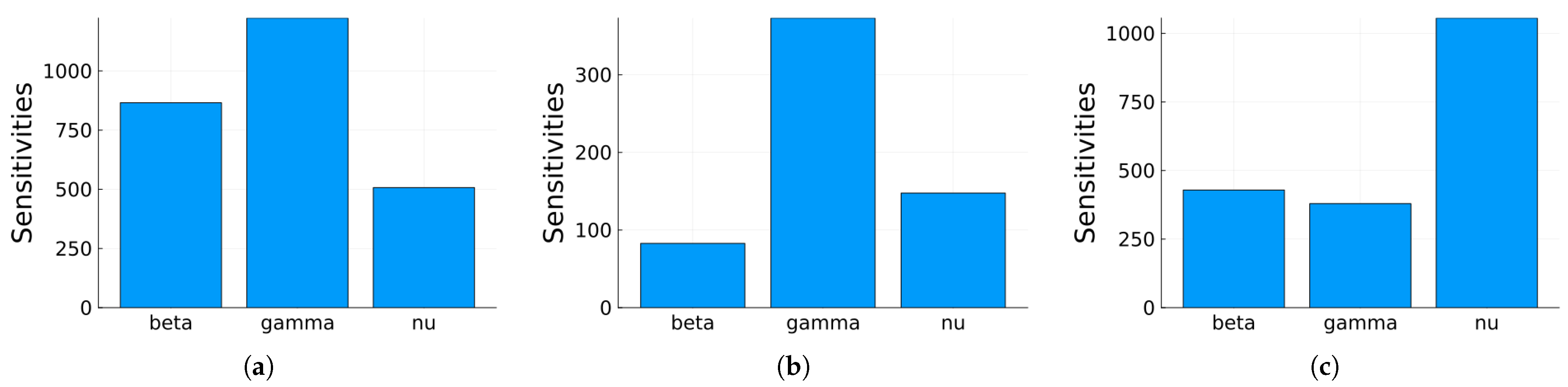
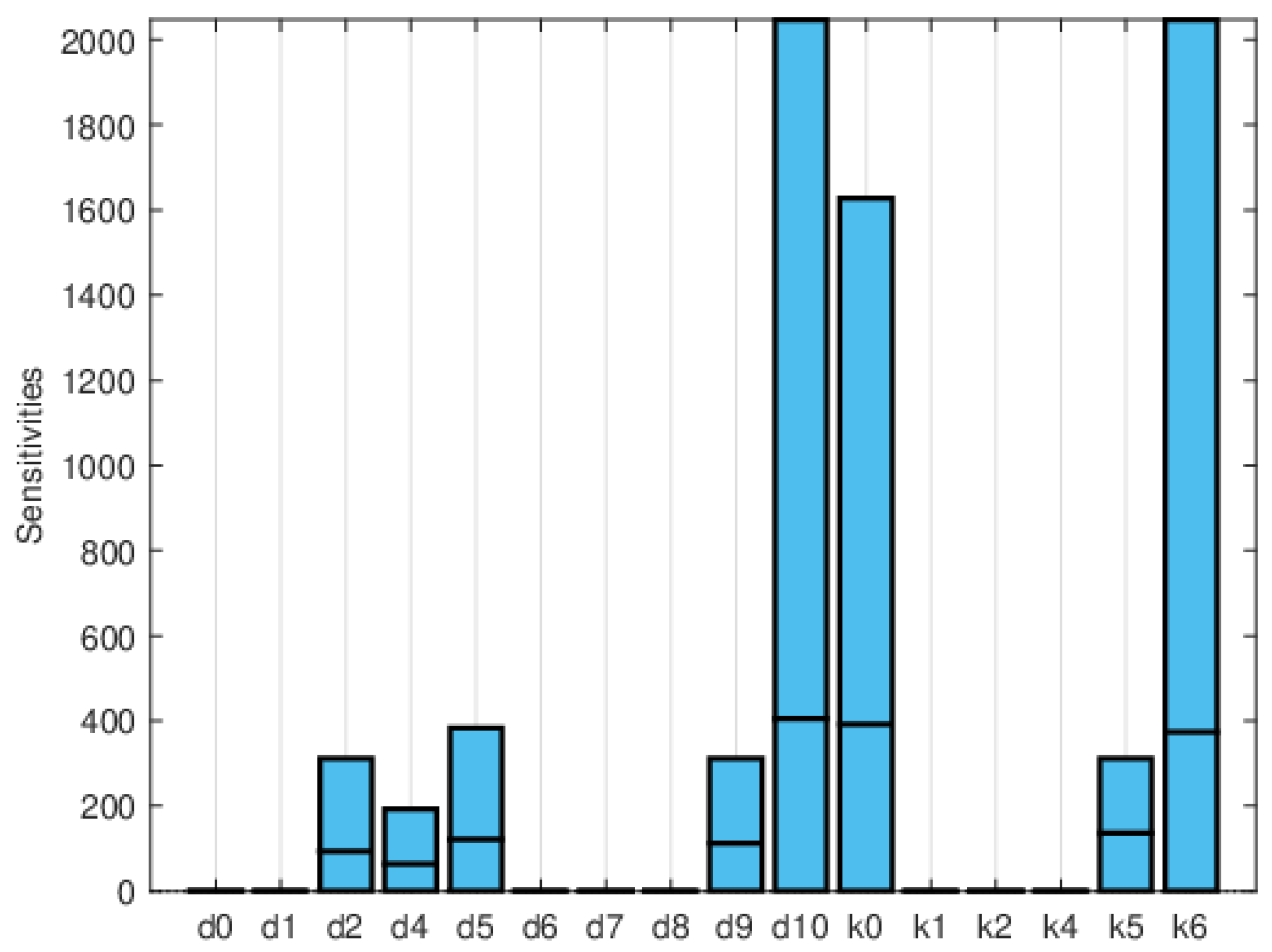
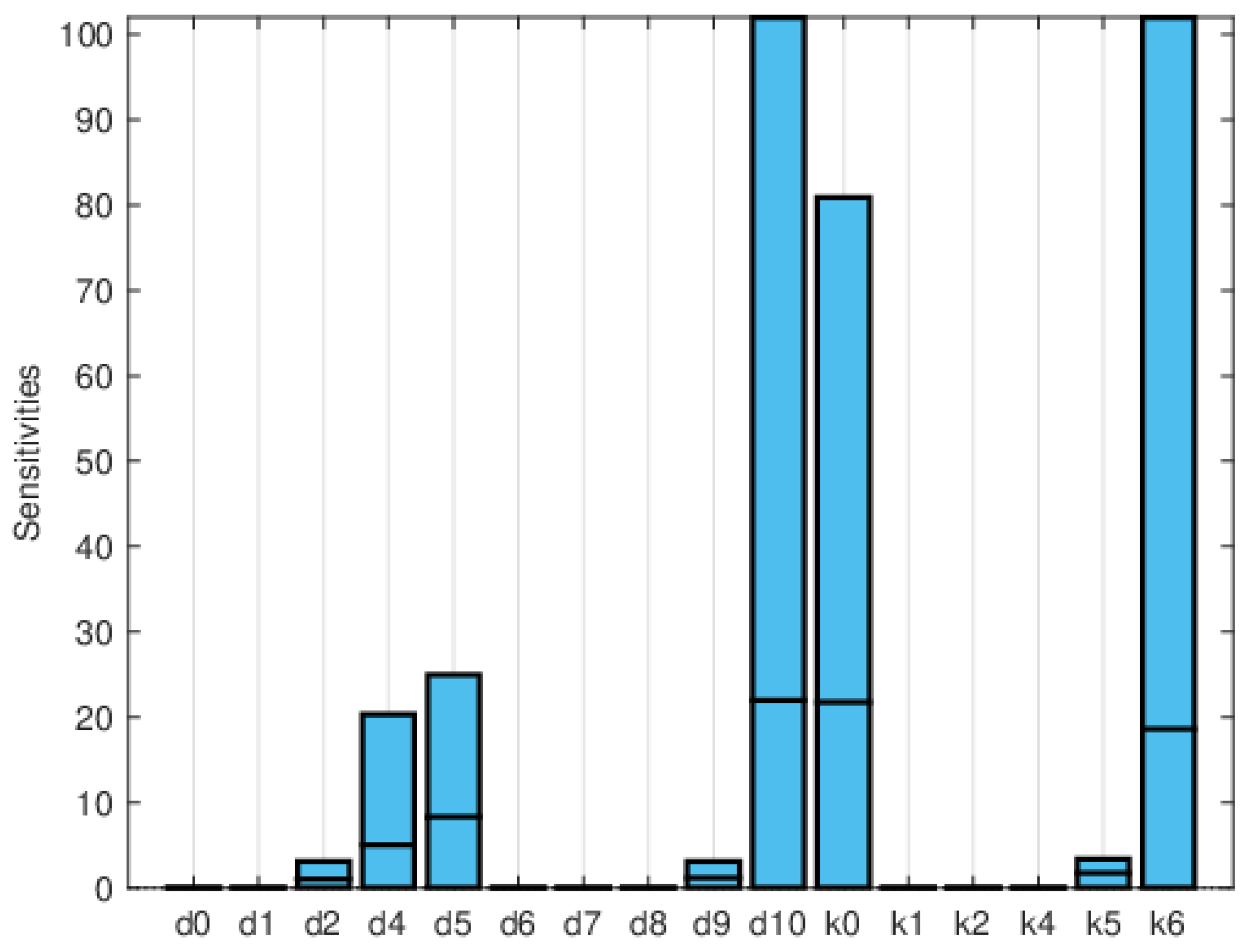
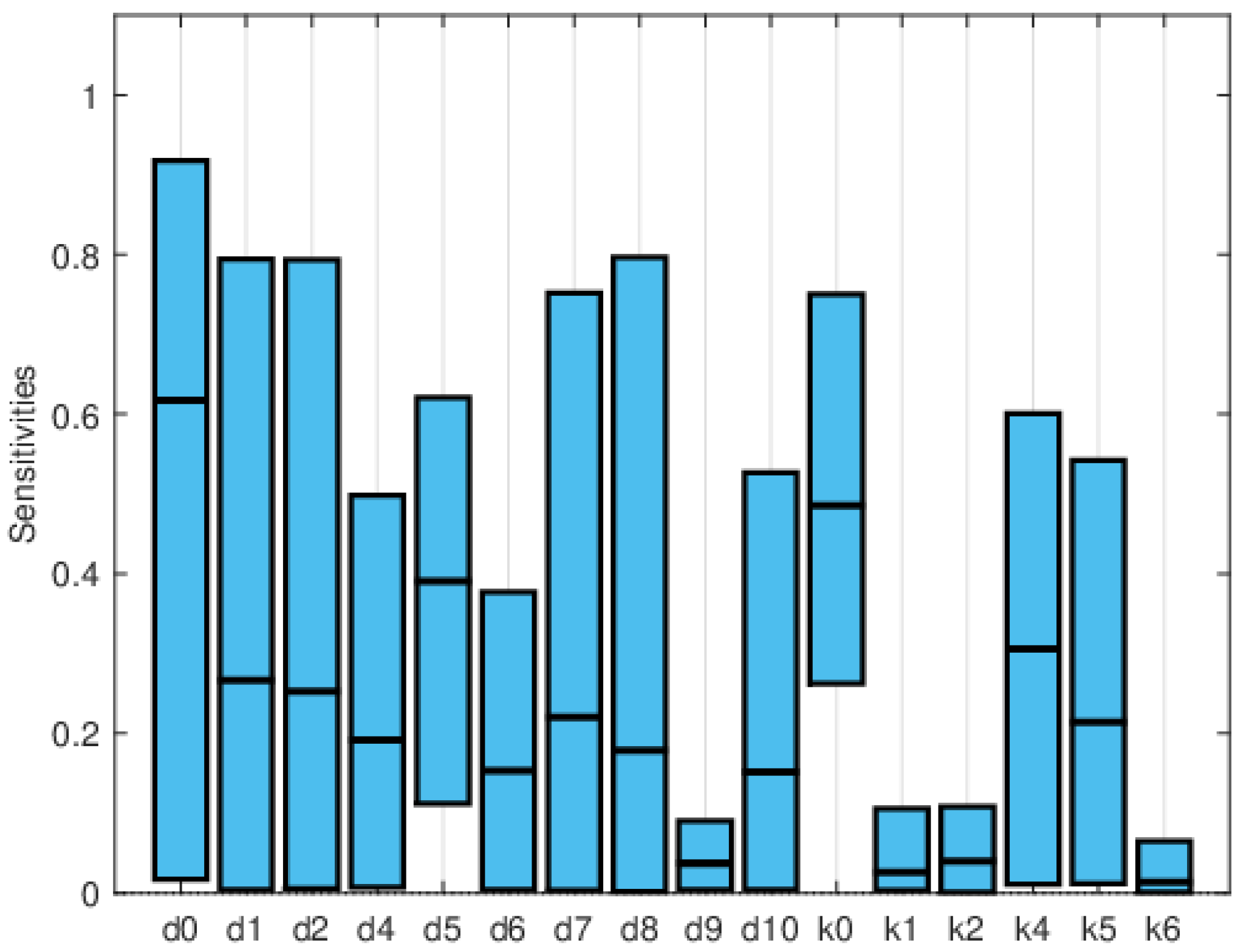
Figure 11, Figure 12 and Figure 13 depict the normalized local sensitivity indices at 15 days, 30 days, and averaged over 30 days, respectively. The top line of each bar corresponds to the maximum, the middle line to the mean, and the bottom line to the minimum values of the local sensitivity indices for all state variables with respect to each parameter. As can be seen, they are very similar in shape, even though their values are very different in each plot. Note that by 30 days, the solution is very close to the steady solution, but since it is still non-zero, the errors are still small. These results suggest that a good strategy for time-dependent sensitivity indices is to use the average over the time period of interest.
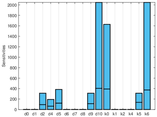
Figure 11.
Plot of the maximum, mean, and minimum values of the local sensitivity indices at 15 days for all state variables with respect to each parameter.
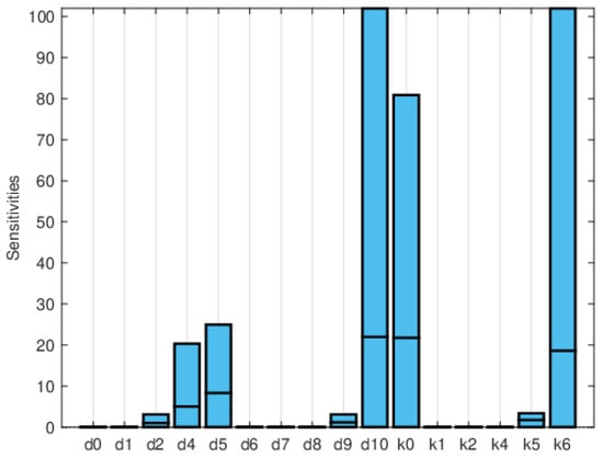
Figure 12.
Plot of the maximum, mean, and minimum values of the local sensitivity indices at 30 days for all state variables with respect to each parameter.
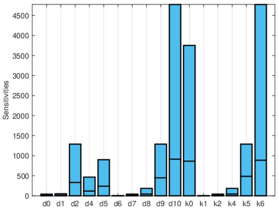
Figure 13.
Plot of the maximum, mean, and minimum values of the local sensitivity indices averaged over time for all state variables with respect to each parameter.
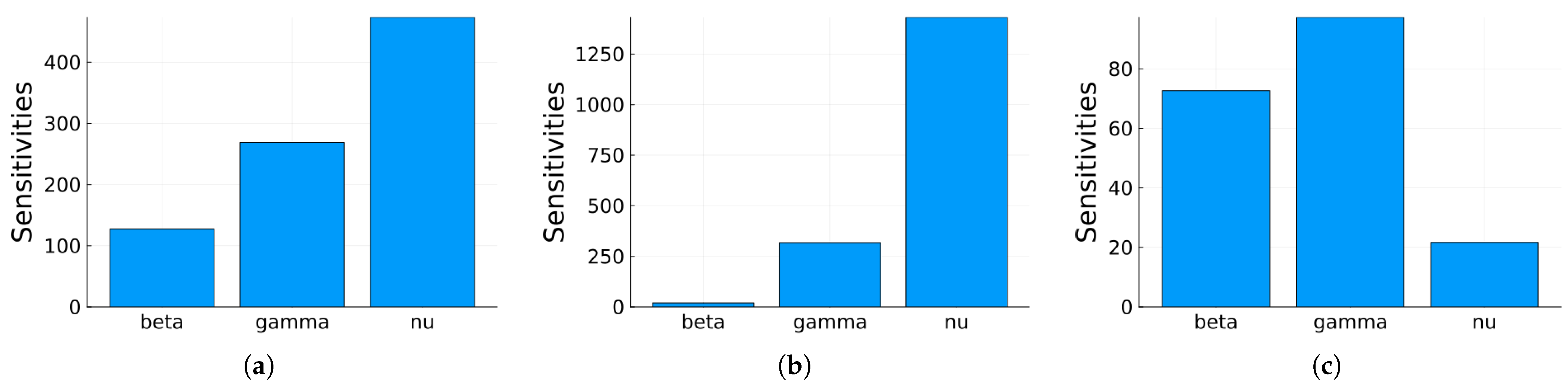
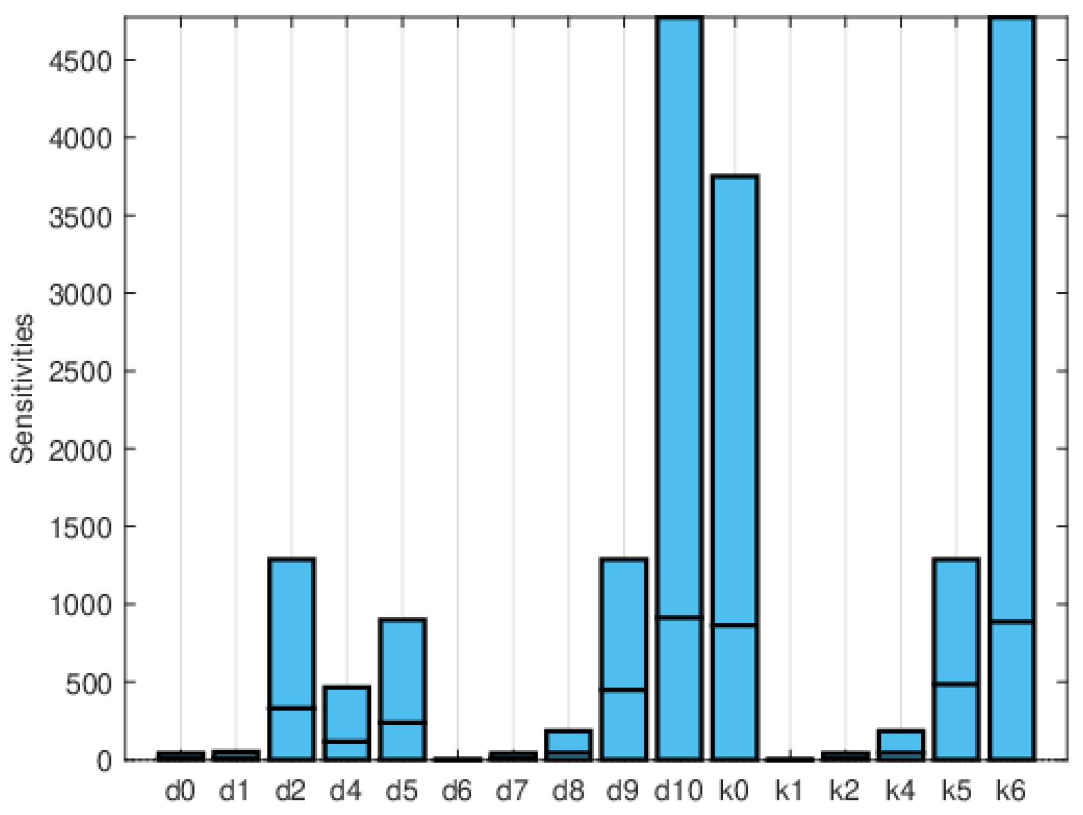
Global sensitivity indices were calculated using the Sobol, FAST, and PRCC methods. All parameters were assumed to have uniform distributions, with minimum values equal to 0.75 times the values in Table 2 and maximum values equal to 1.25 times those in the same table. We did not have access to enough data to estimate these distributions, so they are purely illustrative. Figure 14, Figure 15 and Figure 16 show the sensitivity indices for the PRCC, FAST, and Sobol methods, respectively. Figure 11, Figure 12 and Figure 13 show that the larger local sensitivity indices are for and . In Figure 15 for Sobol’s method and Figure 16 for the FAST method, the largest global sensitivity indices are for and . Figure 14 shows that the PRCC method yields different, larger indices compared to the Sobol and FAST methods. The global indices calculated using the Sobol and FAST methods were the most accurate since they explored the whole range of interest for the parameters. As expected, the PRCC method was not accurate. But since sampling points vary, it is important to use two methods that reasonably agree. Also, the number of sampling points should be varied, and if necessary, bootstrapping should be used. For our model, calculations started with 3000 simulations, and this number was doubled twice. The most important indices changed by less than 10%. The relative size of the indices is what is most relevant.
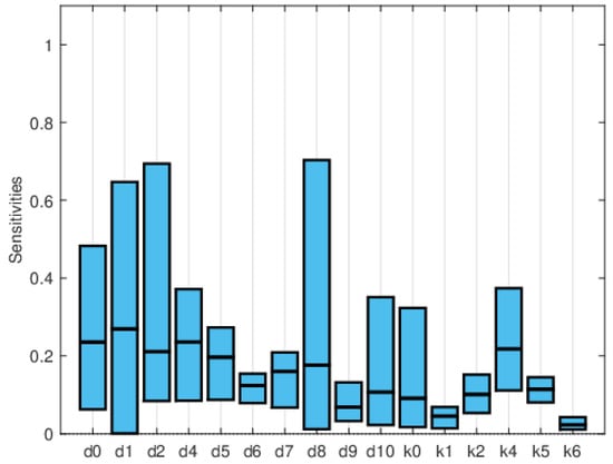
Figure 14.
Maximum, mean, and minimum values of the global sensitivity indices averaged over time using the PRCC method.

Figure 15.
Maximum, mean, and minimum values of the global sensitivity indices averaged over time using the FAST method.
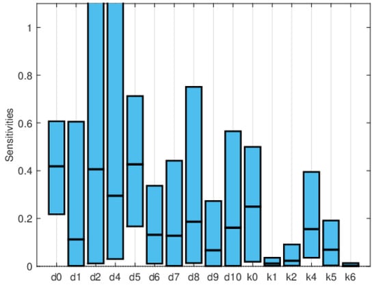
Figure 16.
Maximum, mean, and minimum values of the global sensitivity indices averaged over time using Sobol’s method.
The computational cost rapidly increases with the number of state variables and parameters. Local sensitivity indices are only reliable if the parameter values are accurately known, since for the simple SIRS model, the relative importance of the indices changes with the parameter values. Usually, it is not straightforward to determine if there is interaction between the effects of the parameters, so methods that use one-at-a-time sampling may not yield good results. The monotonicity requirement of the PRCC method may also be hard to establish. The most robust methods are the Sobol and the FAST methods. The number of sensitivity indices increases with the complexity of the model. Focusing only on the indices of an important variable or two is a way to greatly reduce the number of indices. But since the sensitivity indices can also indicate errors or incorrect assumptions if they are relatively large, or suggest possible simplifications to the model if they are very small, it is important to look at all the indices or identify the largest and smallest.
3.2.1. Numerical Simulations
The simulations were performed using the numerical integrator Runge–Kutta–Felhberg 45, implemented in GNU octave.
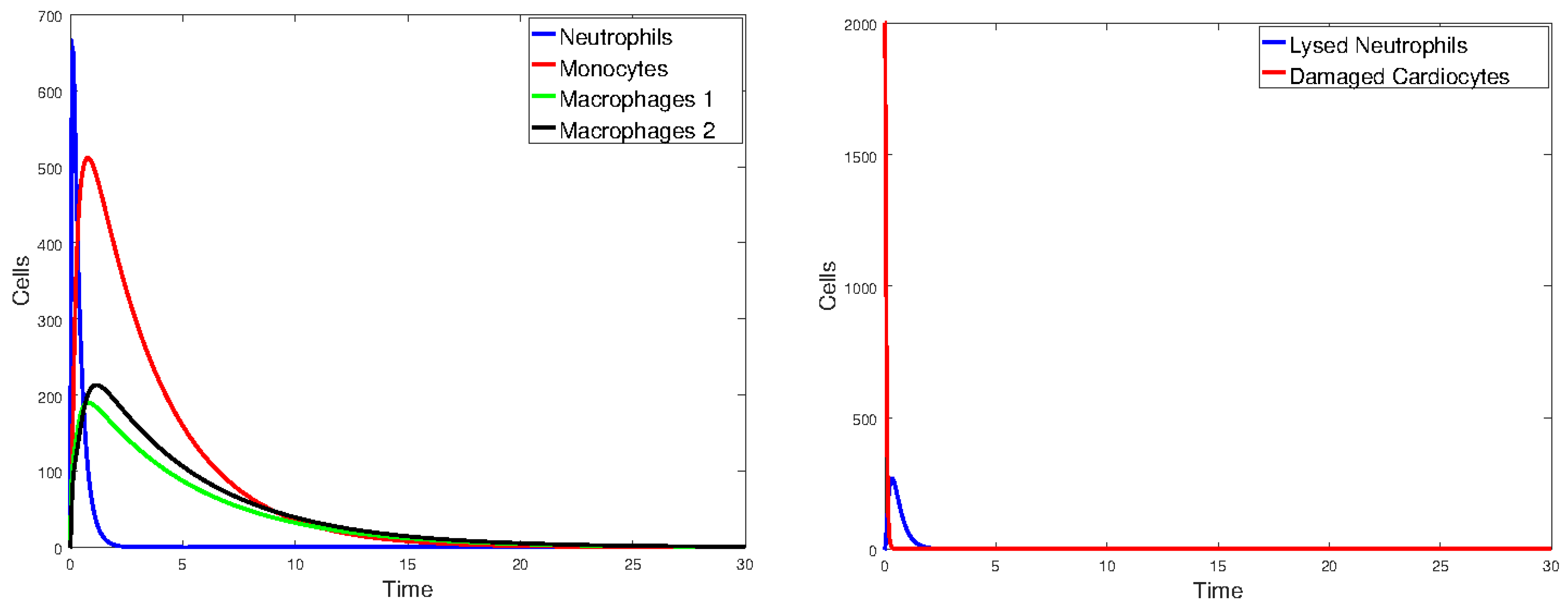
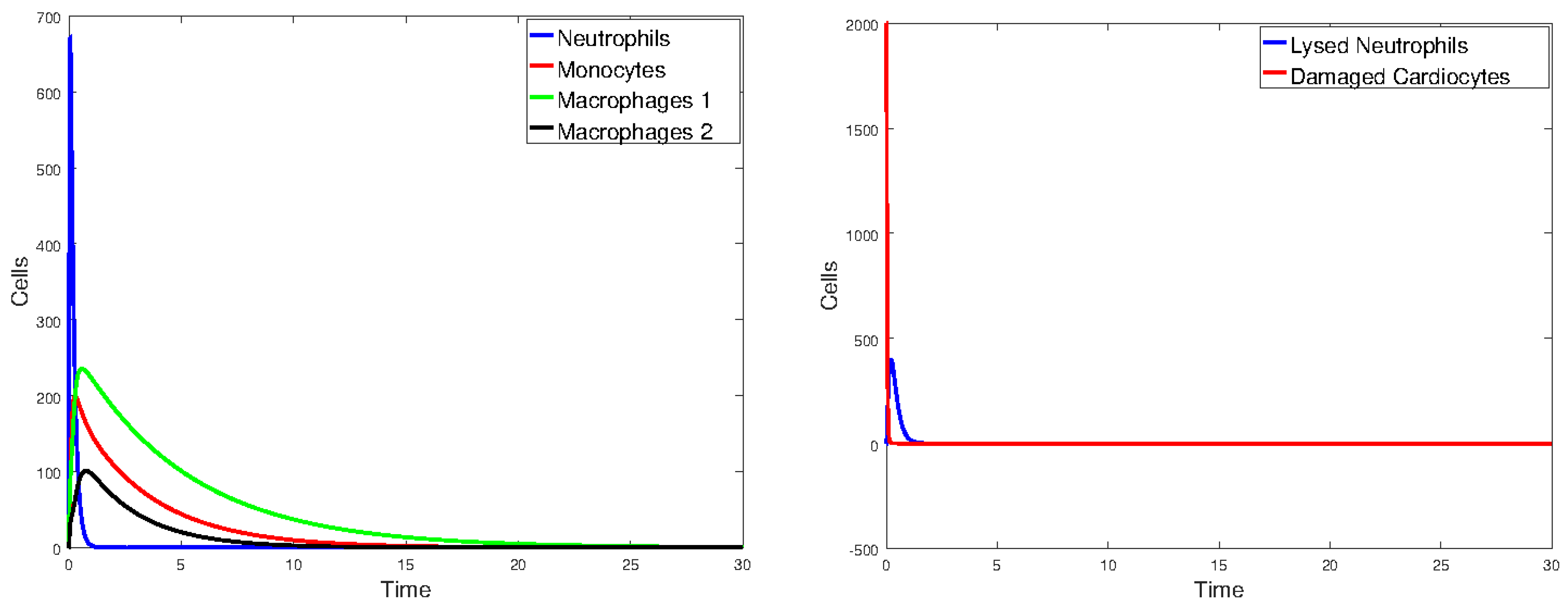
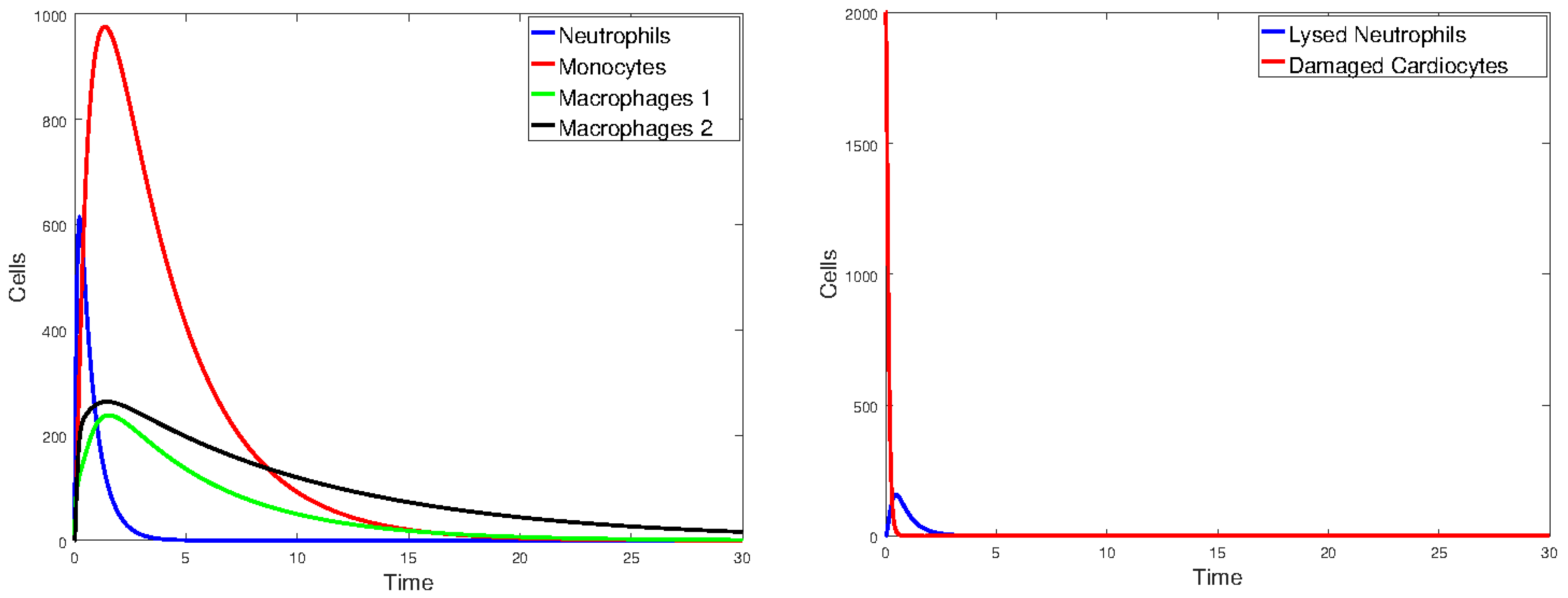
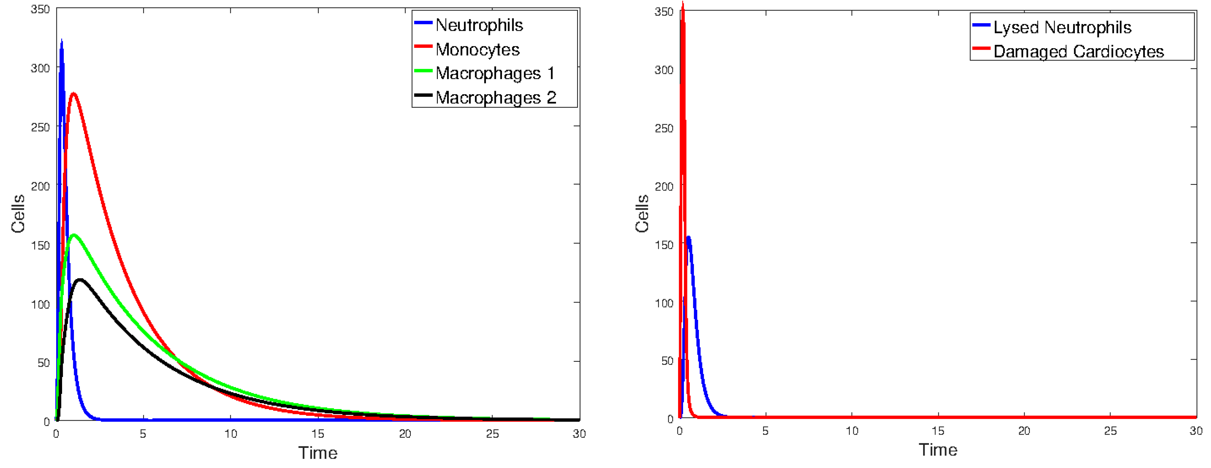
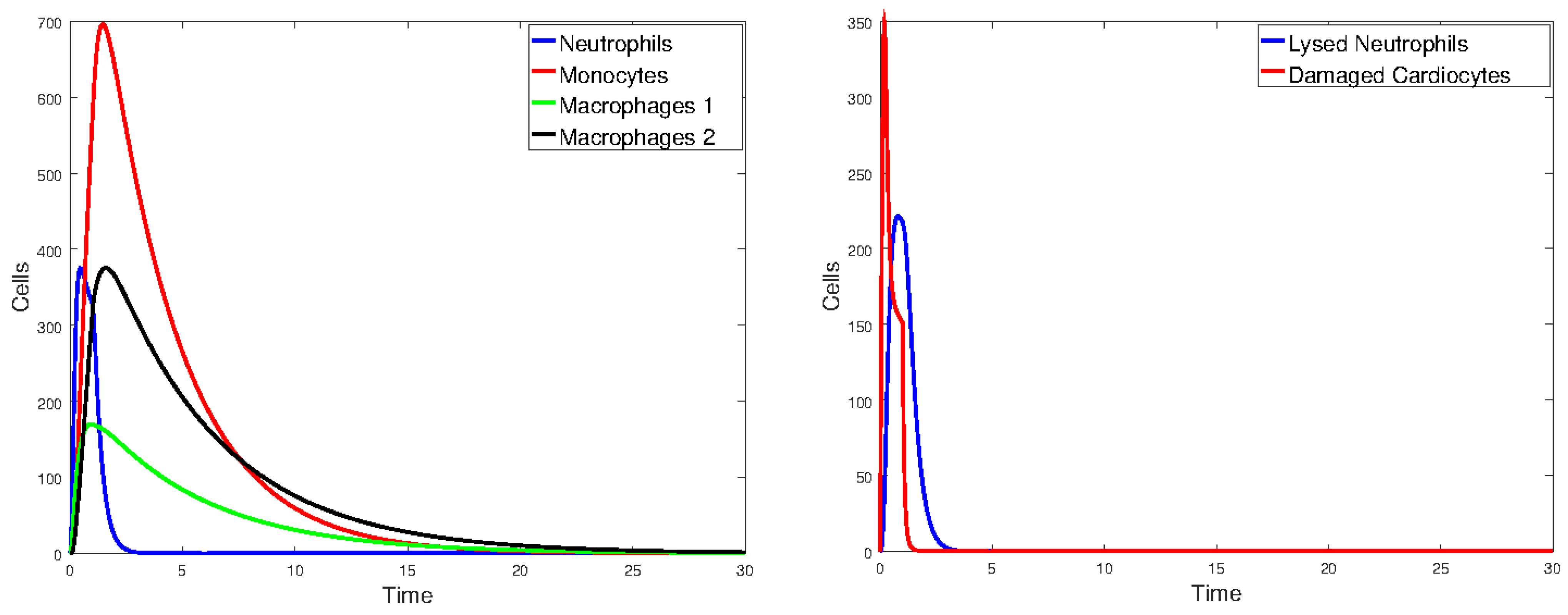
Figure 17 plots the values of all cell populations as functions of time for Model 1 with the values given in Table 2. Figure 18 and Figure 19 show the number of cells versus time after doubling and halving the values of and , which are the parameters that Sobol’s method identified as having the largest impact on cell population changes. The simulations show that changing the values of the parameters with the greatest sensitivity indices by a factor of 2 significantly changes the number of cells and the time it takes the immune cells to eliminate the dead cells.
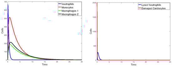
Figure 17.
Plot of all state variables of Model 1. Initial values: all zero, except for , which is 25% of the number of healthy cardiomyocytes. The parameter values are the same as those given in Table 2.

Figure 18.
Plot of all state variables of Model 1. Initial values: all zero, except for , which is 25% of the number of healthy cardiomyocytes. The parameter values are the same as those in Table 2, except that and are doubled.
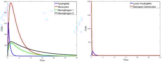
Figure 19.
Plot of all state variables of Model 1. Initial values: all zero, except for , which is 25% of the number of healthy cardiomyocytes. The parameter values are the same as those in Table 2, except that and are halved.
For simulations using Model 2, we used the same parameter values as for Model 1, as given in Table 2, only adding the death rate of cardiomyocytes due to lack of oxygen, . The unit of this parameter was 1/day. The initial conditions were since we started with a healthy heart and cut off the flow of oxygen at time .
We varied the time elapsed before the flow of oxygen was restored from 0.1 day to 1 day. Figure 20 shows the populations when oxygen was restored after days. The plot for C is not shown since it decayed exponentially for days and then remained constant. Figure 21 shows the populations when the oxygen was restored after one day. As expected, the longer it took to restore the flow of oxygen to the heart, the greater the number of dead cardiomyocytes and, of course, the longer it took for neutrophils and macrophages to clean up the dead cells.
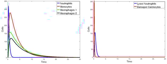
Figure 20.
Plots of the state variables for Model 2. Initial values: all zero, except for cells and day.
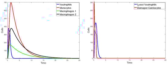
Figure 21.
Plots of the state variables for Model 2. Initial values: all zero, except for cells and day.
3.2.2. Stochastic and Random Differential Equations
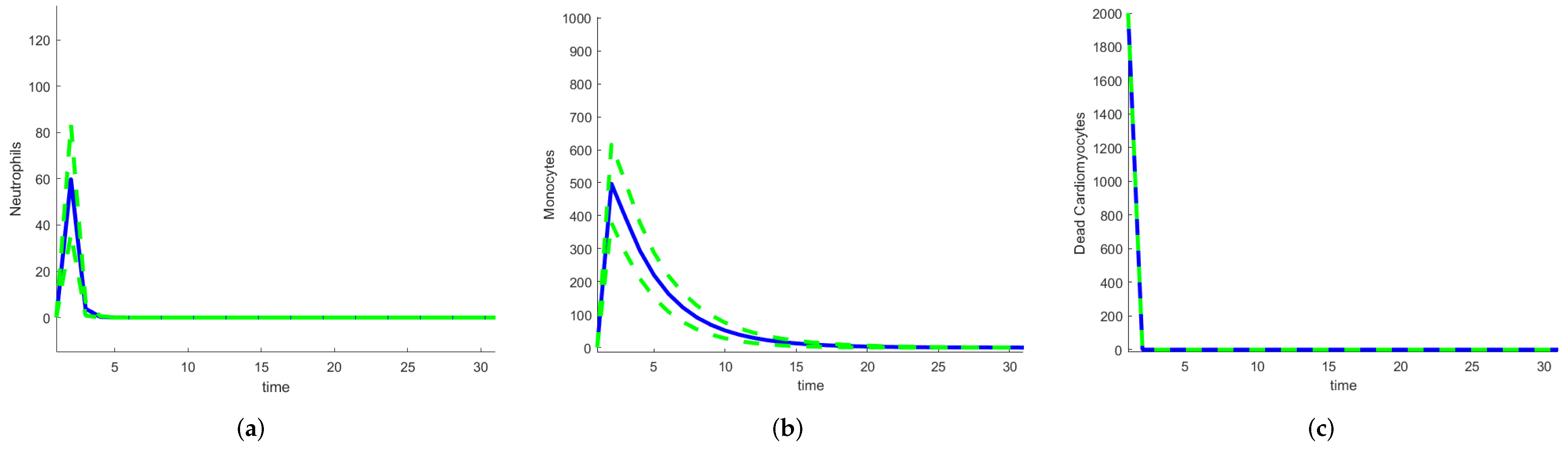
To quantify the uncertainty in the outputs of the model, stochastic and random differential equations can be used. The higher the number of random parameters, the higher the number of realizations required. Model 1 has 16 parameters, so reducing the number of random parameters is important. One route involves using SDEs with only the parameters that have larger sensitivity indices as random variables. For Model 1, this includes , and , so realizations need to be performed by sampling over a space of dimension 4 instead of 16. But even this step is unnecessary. For the calculation of the Sobol or FAST indices, the ODE system needs to be solved using parameter values sampled across their ranges. All the solutions are realizations of the solution of the corresponding random differential equations and can estimate their means and variances (or standard deviations). The calculation of global indices using a method that samples over the parameter space gives an estimate of the uncertainty in the outputs of the model with very little extra work. For Model 1, we used the Sobol indices. Figure 22 shows the mean and the mean ± the standard deviation for neutrophils, monocytes, and dead cardiomyocytes. For dead cardiomyocytes, the standard deviation is very small compared with the number of dead cells.
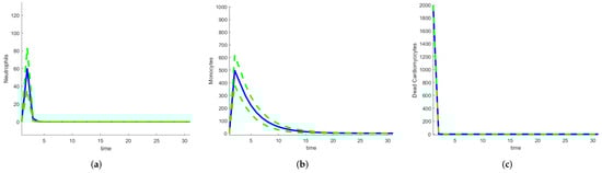
Figure 22.
Mean and mean ± standard deviation for heart infarction Model 1: (a) Neutrophils. (b) Monocytes. (c) Dead cardiomyocytes.
4. Discussion
It is important to determine the reliability of a mathematical model and quantify the uncertainty in its outputs. Many papers dealing with models in mathematical biology include sensitivity analysis, since the values of the parameters, and maybe even the working hypotheses, have large variations. Although more computationally expensive, it is safer to use a global method that samples the parameter space by varying all parameters at the same time, like Sobol’s method and the FAST method. As the complexity of the model increases, so does the computational cost and the number of sensitivity indices. Focusing only on the indices of an important variable or two simplifies the analysis. But it is also important to assess whether some indices are relatively large or small, which may indicate errors or suggest possible simplifications to the model (also see the paper by Saltelli et al. [93]).
In this paper, we compared the indices calculated using a local direct method and several global methods. For the SIRS model, figures are included, showing that the relative importance of the indices is preserved after averaging over time. In the heart infarction model, there are 96 time-dependent indices. From the plots, the larger indices can be discerned, but it is simpler to look at the time averages. For the SIRS model with six indices, their relative importance is now easy to determine, but averaging across states for each parameter can also be considered. In the more complex heart infarction model, we looked at the indices of dead cardiomyocytes and the mean, maximum, and minimum values across the state variables. Knowing which parameters correspond to the largest indices can help guide experimental research to determine or estimate them more accurately. For the heart model one of the most relevant parameters, , is related to neutrophils clearing dead cardiomyocytes. So, a possible additional treatment after MI is to stimulate the production of neutrophils. The uncertainty in the outputs of a mathematical model based on ODEs can be estimated by writing the model in terms of SDEs or RODEs and performing realizations to estimate the mean and variance of the outputs. Sensitivity analysis can help determine which parameters have the largest values by considering those parameters to have a white noise component. More importantly, when using a global method like Sobol’s method or the FAST method, which sample the parameter space by varying all the parameters at the same time, we obtain realizations of the solutions of the corresponding RODE. These realizations can then be used to calculate means and variances.
The SIRS model is very well studied and was used here only to illustrate the differences between the sensitivity analysis methods and how to use the sensitivity analysis results to estimate uncertainty in the outputs.
The heart infarction models describe the quantitative interactions of the immune system and dead cardiomyocytes after myocardial infarction. Model 1 has only one steady solution where all populations are zero, and this solution is stable. Biologically, it means that all dead cardiomyocytes are removed. For , Model 2 has the same zero solution as Model 1 with the exception that the added state variable, the number of live cardiomyocytes, is a constant. Sensitivity analysis shows that variations in parameter values can result in significant changes in the outputs of the model. In particular, the sensitivity indices show that the values of the phagocytosis rates are very important. The results of Sobol’s method and the FAST method are similar. This validates both sets of indices. But the PRCC method yields different relevant indices. Numerical simulations were performed, and their outputs show that varying some parameters by a factor of two significantly changes the values of cell populations and the time it takes the neutrophils and macrophages to eliminate the dead cells. Therefore, there is a need for empirical work to accurately measure these parameters. Of course, population variability will always be a factor. A final, although obvious, conclusion is that restoring oxygen as soon as possible is critical. While there are still no conclusive results on successful treatments, some papers on heart infarction models that include treatment are [94,95].
Author Contributions
Conceptualization, B.C.-C. and H.K.; methodology, B.C.-C.; software, B.C.-C. and H.K.; formal analysis, B.C.-C. and H.K.; investigation, B.C.-C. and H.K.; writing—original draft preparation, B.C.-C. and H.K.; writing—review and editing, B.C.-C. and H.K.; visualization, B.C.-C. and H.K. All authors have read and agreed to the published version of the manuscript.
Funding
This research received no external funding.
Data Availability Statement
The original contributions presented in the study are included in the article, further inquiries can be directed to the corresponding author.
Conflicts of Interest
The authors declare no conflicts of interest.
Abbreviations
The following abbreviations were used in this manuscript:
| MDPI | Multidisciplinary Digital Publishing Institute |
| DOAJ | Directory of open access journals |
| ODE | ordinary differential equation |
| SDE | stochastic differential equation |
| RODE | random ordinary differential equation |
| SIRS | Susceptible–Infective–Recovered–Susceptible |
| MI | myocardial infarction |
| DFE | disease-free equilibrium |
| basic reproduction number | |
| PRCC | partial rank correlation coefficient |
| FAST | Fourier amplitude sensitivity test |
| EFAST | extended Fourier amplitude sensitivity test |
References
- Borgonovo, E.; Plischke, E. Sensitivity analysis: A review of recent advances. Eur. J. Oper. Res. 2016, 248, 869–887. [Google Scholar] [CrossRef]
- Christopher Frey, H.; Patil, S.R. Identification and review of sensitivity analysis methods. Risk Anal. 2002, 22, 553–578. [Google Scholar] [CrossRef]
- Saltelli, A.; Tarantola, S.; Campolongo, F.; Ratto, M. Sensitivity Analysis in Practice: A Guide to Assessing Scientific Models; Wiley Online Library: Hoboken, NJ, USA, 2004; Volume 1. [Google Scholar]
- Pianosi, F.; Beven, K.; Freer, J.; Hall, J.W.; Rougier, J.; Stephenson, D.B.; Wagener, T. Sensitivity analysis of environmental models: A systematic review with practical workflow. Environ. Model. Softw. 2016, 79, 214–232. [Google Scholar] [CrossRef]
- Qian, G.; Mahdi, A. Sensitivity analysis methods in the biomedical sciences. Math. Biosci. 2020, 323, 108306. [Google Scholar] [CrossRef]
- Iwanaga, T.; Usher, W.; Herman, J. Toward SALib 2.0: Advancing the accessibility and interpretability of global sensitivity analyses. Socio-Environ. Syst. Model. 2022, 4, 18155. [Google Scholar] [CrossRef]
- Dai, H.; Liu, Y.; Guadagnini, A.; Yuan, S.; Yang, J.; Ye, M. Comparative assessment of two global sensitivity approaches considering model and parameter uncertainty. Water Resour. Res. 2024, 60, e2023WR036096. [Google Scholar] [CrossRef]
- Razavi, S.; Jakeman, A.; Saltelli, A.; Prieur, C.; Iooss, B.; Borgonovo, E.; Plischke, E.; Piano, S.L.; Iwanaga, T.; Becker, W.; et al. The future of sensitivity analysis: An essential discipline for systems modeling and policy support. Environ. Model. Softw. 2021, 137, 104954. [Google Scholar] [CrossRef]
- Meiler, S.; Ciullo, A.; Kropf, C.M.; Emanuel, K.; Bresch, D.N. Uncertainties and sensitivities in the quantification of future tropical cyclone risk. Commun. Earth Environ. 2023, 4, 371. [Google Scholar] [CrossRef]
- Vermeulen-Miltz, E.; Clifford-Holmes, J.K.; Scharler, U.M.; Lombard, A.T. A system dynamics model to support marine spatial planning in Algoa Bay, South Africa. Environ. Model. Softw. 2023, 160, 105601. [Google Scholar] [CrossRef]
- Moallemi, E.A.; Kwakkel, J.; de Haan, F.J.; Bryan, B.A. Exploratory modeling for analyzing coupled human-natural systems under uncertainty. Glob. Environ. Chang. 2020, 65, 102186. [Google Scholar] [CrossRef]
- Douglas-Smith, D.; Iwanaga, T.; Croke, B.F.; Jakeman, A.J. Certain trends in uncertainty and sensitivity analysis: An overview of software tools and techniques. Environ. Model. Softw. 2020, 124, 104588. [Google Scholar] [CrossRef]
- Rounsevell, M.D.; Arneth, A.; Brown, C.; Cheung, W.W.; Gimenez, O.; Holman, I.; Leadley, P.; Luján, C.; Mahevas, S.; Maréchaux, I.; et al. Identifying uncertainties in scenarios and models of socio-ecological systems in support of decision-making. One Earth 2021, 4, 967–985. [Google Scholar] [CrossRef]
- Puy, A.; Beneventano, P.; Levin, S.A.; Lo Piano, S.; Portaluri, T.; Saltelli, A. Models with higher effective dimensions tend to produce more uncertain estimates. Sci. Adv. 2022, 8, eabn9450. [Google Scholar] [CrossRef]
- Soong, T.T.; Bogdanoff, J. Random Differential Equations in Science and Engineering; Academic Press: Cambridge, MA, USA, 1974. [Google Scholar]
- Ghanem, R.G.; Spanos, P.D. Stochastic Finite Elements: A Spectral Approach; Courier Corporation: Washington, DC, USA, 2003. [Google Scholar]
- Xiu, D.; Karniadakis, G.E. The Wiener–Askey polynomial chaos for stochastic differential equations. SIAM J. Sci. Comput. 2002, 24, 619–644. [Google Scholar] [CrossRef]
- Chen-Charpentier, B.M.; Stanescu, D. Epidemic models with random coefficients. Math. Comput. Model. 2010, 52, 1004–1010. [Google Scholar] [CrossRef]
- Cortés, J.C.; Romero, J.V.; Roselló, M.D.; Santonja, F.J.; Villanueva, R.J. Solving continuous models with dependent uncertainty: A computational approach. Abstr. Appl. Anal. 2013, 2013, 983839. [Google Scholar]
- Oksendal, B. Stochastic Differential Equations: An Introduction with Applications; Springer Science & Business Media: Berlin/Heidelberg, Germany, 2013. [Google Scholar]
- Friedman, A. Stochastic differential equations and applications. In Stochastic Differential Equations; Springer: Berlin/Heidelberg, Germany, 1975; pp. 75–148. [Google Scholar]
- Evans, L.C. An Introduction to Stochastic Differential Equations; American Mathematical Society: Rhode Island, RI, USA, 2012; Volume 82. [Google Scholar]
- Allen, L.J. An Introduction to Stochastic Processes with Applications to Biology; CRC Press: Boca Raton, FL, USA, 2010. [Google Scholar]
- Boettiger, C. From noise to knowledge: How randomness generates novel phenomena and reveals information. Ecol. Lett. 2018, 21, 1255–1267. [Google Scholar] [CrossRef]
- Constable, G.W.; Rogers, T.; McKane, A.J.; Tarnita, C.E. Demographic noise can reverse the direction of deterministic selection. Proc. Natl. Acad. Sci. USA 2016, 113, E4745–E4754. [Google Scholar] [CrossRef]
- Zaikin, A.; Kurths, J. Additive noise in noise-induced nonequilibrium transitions. Chaos Interdiscip. J. Nonlinear Sci. 2001, 11, 570–580. [Google Scholar] [CrossRef]
- Allen, E. Modeling with Itô Stochastic Differential Equations; Springer Science & Business Media: Berlin/Heidelberg, Germany, 2007; Volume 22. [Google Scholar]
- Allen, E.J.; Allen, L.J.; Arciniega, A.; Greenwood, P.E. Construction of equivalent stochastic differential equation models. Stoch. Anal. Appl. 2008, 26, 274–297. [Google Scholar] [CrossRef]
- Edelstein-Keshet, L. Mathematical Models in Biology; SIAM: Philadelphia, PA, USA, 2005. [Google Scholar]
- Allen, L. An Introduction to Mathematical Biology; Pearson-Prentice Hall: Upper Saddle River, NJ, USA, 2007. [Google Scholar]
- Chen-Charpentier, B.; Kojouharov, H. Mathematical Modeling of Myocardial Infarction. Model. Eng. Hum. Behav. 2019, 46, 1–216. [Google Scholar]
- WHO. The Atlas of Heart Disease and Stroke; WHO: Geneva, Switzerland, 2004. [Google Scholar]
- Anderson, J.L.; Morrow, D.A. Acute Myocardial Infarction. N. Engl. J. Med. 2017, 376, 2053–2064. [Google Scholar] [CrossRef] [PubMed]
- Terjung, R.; Frangogiannis, N.G. Pathophysiology of Myocardial Infarction; John Wiley and Sons: Hoboken, NJ, USA, 2013; pp. 313–1875. [Google Scholar]
- Ambrose, J.; Singh, M. Pathophysiology of coronary artery disease leading to acute coronary syndromes. F1000Prime Rep. 2015, 7, 8. [Google Scholar] [CrossRef] [PubMed]
- Betts, J.G. Anatomy and Physiology; OpenStax College, Rice University: Houston, TX, USA, 2013. [Google Scholar]
- Jackson, K.A.; Majka, S.M.; Wang, H.; Pocius, J.; Hartley, C.J.; Majesky, M.W.; Entman, M.L.; Michael, L.H.; Hirschi, K.K.; Goodell, M.A. Regeneration of ischemic cardiac muscle and vascular endothelium by adult stem cells. J. Clin. Investig. 2001, 107, 1395–1402. [Google Scholar] [CrossRef] [PubMed]
- Hethcote, H.W. The mathematics of infectious diseases. SIAM Rev. 2000, 42, 599–653. [Google Scholar] [CrossRef]
- Van den Driessche, P.; Watmough, J. Reproduction numbers and sub-threshold endemic equilibria for compartmental models of disease transmission. Math. Biosci. 2002, 180, 29–48. [Google Scholar] [CrossRef] [PubMed]
- Gray, G.; Toor, I.; Castellan, R.; Crisan, M.; Meloni, M. Resident cells of the myocardium: More than spectators in cardiac injury, repair and regeneration. Curr. Opin. Physiol. 2018, 1, 46–51. [Google Scholar] [CrossRef] [PubMed]
- Nahrendorf, M.; Swirski, F.K. Monocyte and Macrophage Heterogeneity in the Heart. Circ. Res. 2013, 112, 1624–1633. [Google Scholar] [CrossRef] [PubMed]
- Roszer, T. Understanding the Mysterious M2 Macrophage through Activation Markers and Effector Mechanisms. Mediat. Inflamm. 2015, 2015, 816460. [Google Scholar] [CrossRef] [PubMed]
- Bonvini, R.F.; Hendiri, T.; Camenzind, E. Inflammatory response post-myocardial infarction and reperfusion: A new therapeutic target? Eur. Heart J. Suppl. 2005, 7, I27–I36. [Google Scholar] [CrossRef]
- Chen, B.; Frangogiannis, N.G. Immune cells in repair of the infarcted myocardium. Microcirculation 2017, 24, e12305. [Google Scholar] [CrossRef]
- Fang, L.; Moore, X.L.; Dart, A.M.; Wang, L.M. Systemic inflammatory response following acute myocardial infarction. J. Geriatr. Cardiol. JGC 2015, 12, 305. [Google Scholar] [PubMed]
- Saparov, A.; Ogay, V.; Nurgozhin, T.; Chen, W.C.W.; Mansurov, N.; Issabekova, A.; Zhakupova, J. Role of the immune system in cardiac tissue damage and repair following myocardial infarction. Inflamm. Res. 2017, 66, 739–751. [Google Scholar] [CrossRef] [PubMed]
- Swirski, F.K.; Nahrendorf, M. Cardioimmunology: The immune system in cardiac homeostasis and disease. Nat. Rev. Immunol. 2018, 18, 733–744. [Google Scholar] [CrossRef] [PubMed]
- Troidl, C.; Möllmann, H.; Nef, H.; Masseli, F.; Voss, S.; Szardien, S.; Willmer, M.; Rolf, A.; Rixe, J.; Troidl, K.; et al. Classically and alternatively activated macrophages contribute to tissue remodelling after myocardial infarction. J. Cell. Mol. Med. 2009, 13, 3485–3496. [Google Scholar] [CrossRef] [PubMed]
- Frangogiannis, N.G.; Mendoza, L.H.; Lindsey, M.L.; Ballantyne, C.M.; Michael, L.H.; Smith, C.W.; Entman, M.L. IL-10 Is Induced in the Reperfused Myocardium and May Modulate the Reaction to Injury. J. Immunol. 2000, 165, 2798–2808. [Google Scholar] [CrossRef] [PubMed]
- Patti, G.; D’Ambrosio, A.; Mega, S.; Giorgi, G.; Zardi, E.M.; Zardi, D.M.; Dicuonzo, G.; Dobrina, A.; Di Sciascio, G. Early interleukin-1 receptor antagonist elevation in patients with acute myocardial infarction. J. Am. Coll. Cardiol. 2004, 43, 35–38. [Google Scholar] [CrossRef] [PubMed]
- Wang, Y.; Yang, T.; Ma, Y.; Halade, G.V.; Zhang, J.; Lindsey, M.L.; Jin, Y.F. Mathematical modeling and stability analysis of macrophage activation in left ventricular remodeling post-myocardial infarction. BMC Genom. 2012, 13, S21. [Google Scholar] [CrossRef] [PubMed]
- Jin, Y.F.; Han, H.C.; Berger, J.; Dai, Q.; Lindsey, M.L. Combining experimental and mathematical modeling to reveal mechanisms of macrophage-dependent left ventricular remodeling. BMC Syst. Biol. 2011, 5, 60. [Google Scholar] [CrossRef] [PubMed]
- Dunster, J.L.; Byrne, H.M.; King, J.R. The Resolution of Inflammation: A Mathematical Model of Neutrophil and Macrophage Interactions. Bull. Math. Biol. 2014, 76, 1953–1980. [Google Scholar] [CrossRef]
- Dunster, J.L. The macrophage and its role in inflammation and tissue repair: Mathematical and systems biology approaches: Macrophage and its role in inflammation and tissue repair. Wiley Interdiscip. Rev. Syst. Biol. Med. 2016, 8, 87–99. [Google Scholar] [CrossRef]
- Yang, F.; Liu, Y.H.; Yang, X.P.; Xu, J.; Kapke, A.; Carretero, O.A. Myocardial Infarction and Cardiac Remodelling in Mice. Exp. Physiol. 2002, 87, 547–555. [Google Scholar] [CrossRef] [PubMed]
- Perko, L. Differential Equations and Dynamical Systems; Springer Science & Business Media: Berlin/Heidelberg, Germany, 2013. [Google Scholar]
- Dickinson, R.P.; Gelinas, R.J. Sensitivity analysis of ordinary differential equation systems—A direct method. J. Comput. Phys. 1976, 21, 123–143. [Google Scholar] [CrossRef]
- Gustafson, P.; Srinivasan, C.; Wasserman, L. Local sensitivity analysis. Bayesian Stat. 1996, 5, 197–210. [Google Scholar]
- Arriola, L.; Hyman, J.M. Sensitivity analysis for uncertainty quantification in mathematical models. In Mathematical and Statistical Estimation Approaches in Epidemiology; Springer: Berlin/Heidelberg, Germany, 2009; pp. 195–247. [Google Scholar]
- Ma, Y.; Dixit, V.; Innes, M.J.; Guo, X.; Rackauckas, C. A comparison of automatic differentiation and continuous sensitivity analysis for derivatives of differential equation solutions. In Proceedings of the 2021 IEEE High Performance Extreme Computing Conference (HPEC), Virtual, 20–24 September 2021; pp. 1–9. [Google Scholar]
- Rabitz, H. General Sensitivity Analysis of Differential Equation Systems. In Proceedings of the Fluctuations and Sensitivity in Nonequilibrium Systems: Proceedings of an International Conference, Austin, TX, USA, 12–16 March 1984; Springer: Berlin/Heidelberg, Germany, 1984; pp. 196–203. [Google Scholar]
- Saltelli, A.; Ratto, M.; Andres, T.; Campolongo, F.; Cariboni, J.; Gatelli, D.; Saisana, M.; Tarantola, S. Global Sensitivity Analysis: The Primer; John Wiley & Sons: Hoboken, NJ, USA, 2008. [Google Scholar]
- Saltelli, A. Sensitivity analysis: Could better methods be used? J. Geophys. Res. Atmos. 1999, 104, 3789–3793. [Google Scholar] [CrossRef]
- Zhang, X.Y.; Trame, M.N.; Lesko, L.J.; Schmidt, S. Sobol sensitivity analysis: A tool to guide the development and evaluation of systems pharmacology models. CPT Pharmacomet. Syst. Pharmacol. 2015, 4, 69–79. [Google Scholar] [CrossRef] [PubMed]
- Savatorova, V. Exploring Parameter Sensitivity Analysis in Mathematical Modeling with Ordinary Differential Equations. CODEE J. 2023, 16, 4. [Google Scholar]
- Cukier, R.; Fortuin, C.; Shuler, K.E.; Petschek, A.; Schaibly, J.H. Study of the sensitivity of coupled reaction systems to uncertainties in rate coefficients. I Theory. J. Chem. Phys. 1973, 59, 3873–3878. [Google Scholar] [CrossRef]
- Pianosi, F.; Sarrazin, F.; Wagener, T. A Matlab toolbox for global sensitivity analysis. Environ. Model. Softw. 2015, 70, 80–85. [Google Scholar] [CrossRef]
- Dela, A.; Shtylla, B.; de Pillis, L. Multi-method global sensitivity analysis of mathematical models. J. Theor. Biol. 2022, 546, 111159. [Google Scholar] [CrossRef]
- Morris, M.D. Factorial sampling plans for preliminary computational experiments. Technometrics 1991, 33, 161–174. [Google Scholar]
- Marino, S.; Hogue, I.B.; Ray, C.J.; Kirschner, D.E. A methodology for performing global uncertainty and sensitivity analysis in systems biology. J. Theor. Biol. 2008, 254, 178–196. [Google Scholar] [CrossRef] [PubMed]
- Alam, M.S.; Kamrujjaman, M.; Islam, M.S. Parameter sensitivity and qualitative analysis of dynamics of ovarian tumor growth model with treatment strategy. J. Appl. Math. Phys. 2020, 8, 941–955. [Google Scholar] [CrossRef]
- Li, D.; Jiang, P.; Hu, C.; Yan, T. Comparison of local and global sensitivity analysis methods and application to thermal hydraulic phenomena. Prog. Nucl. Energy 2023, 158, 104612. [Google Scholar] [CrossRef]
- Qin, C.; Jin, Y.; Tian, M.; Ju, P.; Zhou, S. Comparative Study of Global Sensitivity Analysis and Local Sensitivity Analysis in Power System Parameter Identification. Energies 2023, 16, 5915. [Google Scholar] [CrossRef]
- Rabitz, H.; Kramer, M.; Dacol, D. Sensitivity analysis in chemical kinetics. Annu. Rev. Phys. Chem. 1983, 34, 419–461. [Google Scholar] [CrossRef]
- Zheng, Y.; Rundell, A. Comparative study of parameter sensitivity analyses of the TCR-activated Erk-MAPK signalling pathway. IEE Proc.-Syst. Biol. 2006, 153, 201–211. [Google Scholar] [CrossRef] [PubMed]
- Serban, R.; Hindmarsh, A.C. CVODES: An ODE Solver with Sensitivity Analysis Capabilities; Technical Report; Technical Report UCRL-JP-200039; Lawrence Livermore National Laboratory: Livermore, CA, USA, 2003.
- Rackauckas, C.; Ma, Y.; Martensen, J.; Warner, C.; Zubov, K.; Supekar, R.; Skinner, D.; Ramadhan, A. Universal differential equations for scientific machine learning. arXiv 2020, arXiv:2001.04385. [Google Scholar]
- MathWorks. odeSensitivity. 2024. Available online: https://www.mathworks.com/help/matlab/ref/odesensitivity.html (accessed on 10 June 2012).
- McKay, M.D.; Beckman, R.J.; Conover, W.J. Comparison of three methods for selecting values of input variables in the analysis of output from a computer code. Technometrics 1979, 21, 239–245. [Google Scholar]
- Kucherenko, S.; Albrecht, D.; Saltelli, A. Exploring multi-dimensional spaces: A comparison of Latin hypercube and quasi Monte Carlo sampling techniques. arXiv 2015, arXiv:1505.02350. [Google Scholar]
- Renardy, M.; Joslyn, L.R.; Millar, J.A.; Kirschner, D.E. To Sobol or not to Sobol? The effects of sampling schemes in systems biology applications. Math. Biosci. 2021, 337, 108593. [Google Scholar] [CrossRef]
- Blower, S.M.; Hartel, D.; Dowlatabadi, H.; Anderson, R.M.; May, R.M. Drugs, sex and HIV: A mathematical model for New York City. Phil. Trans. R. Soc. Lond. B 1991, 331, 171–187. [Google Scholar]
- Xu, C.; Gertner, G. Understanding and comparisons of different sampling approaches for the Fourier Amplitudes Sensitivity Test (FAST). Comput. Stat. Data Anal. 2011, 55, 184–198. [Google Scholar] [CrossRef] [PubMed]
- Pianosi, F.; Sarrazin, F.; Wagener, T. How successfully is open-source research software adopted? Results and implications of surveying the users of a sensitivity analysis toolbox. Environ. Model. Softw. 2020, 124, 104579. [Google Scholar] [CrossRef]
- Dixit, V.K.; Rackauckas, C. GlobalSensitivity.jl: Performant and Parallel Global Sensitivity Analysis with Julia. J. Open Source Softw. 2022, 7, 4561. [Google Scholar] [CrossRef]
- Kloeden, P.E.; Platen, E.; Schurz, H. Numerical Solution of SDE through Computer Experiments; Springer Science & Business Media: Berlin/Heidelberg, Germany, 2012. [Google Scholar]
- Sauer, T. Computational solution of stochastic differential equations. Wiley Interdiscip. Rev. Comput. Stat. 2013, 5, 362–371. [Google Scholar] [CrossRef]
- Higham, D.; Kloeden, P. An Introduction to the Numerical Simulation of Stochastic Differential Equations; SIAM: Philadelphia, PA, USA, 2021. [Google Scholar]
- Colizza, V.; Barrat, A.; Barthelemy, M.; Valleron, A.J.; Vespignani, A. Modeling the worldwide spread of pandemic influenza: Baseline case and containment interventions. PLoS Med. 2007, 4, e13. [Google Scholar] [CrossRef] [PubMed]
- Centers for Disease Control. Influenza (Flu). 2024. Available online: https://www.cdc.gov/flu/about/keyfacts.htm#:~:text=Flu%20is%20a%20contagious%20respiratory,a%20flu%20vaccine%20each%20year (accessed on 24 April 2012).
- Rackauckas, C.; Nie, Q. DifferentialEquations.jl—A Performant and Feature-Rich Ecosystem for Solving Differential Equations in Julia. J. Open Res. Softw. 2017, 5, 15. [Google Scholar] [CrossRef]
- Olivetti, G. Aging, Cardiac Hypertrophy and Ischemic Cardiomyopathy Do Not Affect the Proportion of Mononucleated and Multinucleated Myocytes in the Human Heart. J. Mol. Cell. Cardiol. 1996, 28, 1463–1477. [Google Scholar] [CrossRef] [PubMed]
- Saltelli, A.; Aleksankina, K.; Becker, W.; Fennell, P.; Ferretti, F.; Holst, N.; Li, S.; Wu, Q. Why so many published sensitivity analyses are false: A systematic review of sensitivity analysis practices. Environ. Model. Softw. 2019, 114, 29–39. [Google Scholar] [CrossRef]
- Lafci Büyükkahraman, M.; Sabine, G.K.; Kojouharov, H.V.; Chen-Charpentier, B.M.; McMahan, S.R.; Liao, J. Using models to advance medicine: Mathematical modeling of post-myocardial infarction left ventricular remodeling. Comput. Methods Biomech. Biomed. Eng. 2022, 25, 298–307. [Google Scholar] [CrossRef]
- Moise, N.; Friedman, A. A mathematical model of immunomodulatory treatment in myocardial infarction. J. Theor. Biol. 2022, 544, 111122. [Google Scholar] [CrossRef] [PubMed]


Disclaimer/Publisher’s Note: The statements, opinions and data contained in all publications are solely those of the individual author(s) and contributor(s) and not of MDPI and/or the editor(s). MDPI and/or the editor(s) disclaim responsibility for any injury to people or property resulting from any ideas, methods, instructions or products referred to in the content. |
© 2024 by the authors. Licensee MDPI, Basel, Switzerland. This article is an open access article distributed under the terms and conditions of the Creative Commons Attribution (CC BY) license (https://creativecommons.org/licenses/by/4.0/).