Nonlinear SIRS Fractional-Order Model: Analysing the Impact of Public Attitudes towards Vaccination, Government Actions, and Social Behavior on Disease Spread

Abstract

This present work develops a nonlinear SIRS fractional-order model with a system of four equations in the Caputo sense. This study examines the impact of positive and negative attitudes towards vaccination, as well as the role of government actions, social behavior and public reaction on the spread of infectious diseases. The local stability of the equilibrium points is analyzed. Sensitivity analysis is conducted to calculate and discuss the sensitivity index of various parameters. It has been established that the illness would spread across this system when the basic reproduction number is larger than 1, the system becomes infection-free when the reproduction number lies below its threshold value of 1. Numerical figures depict the effects of positive and negative attitudes towards vaccination to make the system disease-free sooner. A comprehensive study regarding various values of the order of fractional derivatives together with integer-order derivatives has been discussed in the numerical section to obtain some useful insights into the intricate dynamics of the proposed system. The Pontryagin principle is used in the formulation and subsequent discussion of an optimum control issue. The study also reveals the significant role of government actions in controlling the epidemic. A numerical analysis has been conducted to compare the system’s behavior under optimal control and without optimal control, aiming to discern their differences. The policies implemented by the government are regarded as the most adequate control strategy, and it is determined that the execution of control mechanisms considerably diminishes the ailment burden.

1. Introduction

Fractional calculus can be seen as an extension of traditional calculus, where fractional orders are used instead of integer orders [1,2]. Extensive research has revealed a noteworthy relationship between integer-order models and fractional-order models. It has been observed that integer-order models can be regarded as specific instances or special cases of fractional-order models. As the fractional-order approaches one, the solutions of the fractional-order system are expected to converge toward the solutions obtained from the corresponding integer-order system [3]. As a result, there are numerous domains in which fractional-order systems offer more suitable descriptions than their integer-order counterparts. Specifically, phenomena characterized by ‘memory and influenced by hereditary properties’ present challenges for accurate representation using integer-order systems alone. In such cases, fractional-order systems prove to be more effective in capturing the intricate dynamics and characteristics of these phenomena [2,4,5]. It has been observed that fractional-order systems provide a better fit for real-life data related to such phenomena. The application of fractional-order modeling has demonstrated clear benefits in the field of disease studies, owing to the generalized nature of the fractional derivative compared to the integer-order derivative. Furthermore, while the integer derivative is local in nature, the fractional derivative is global, making it particularly useful for modeling epidemic problems. Moreover, the introduction of fractional-order systems introduces an additional parameter that significantly improves the numerical simulations. In contemporary times, researchers have paid substantial attention to epidemiological modeling utilizing fractional-order derivatives rather than integer-order derivatives [6,7,8,9,10,11,12].

Memory plays a crucial role in the context of epidemics within human society. Whenever a contagious disease spreads, individuals’ knowledge and past experiences of that particular disease influence their response [13]. If people have encountered the disease before, they take precautionary measures, such as vaccination if available. Such actions can help to limit the spread of the disease. However, it is important to note that mere knowledge about a disease does not always guarantee protection from the disease. Consequently, people are motivated to explore new approaches to disease control. The impact of past experiences with an infectious disease significantly affects the current situation compared to having no memory of it. The long-term influence of memory is expected to decline more slowly over time than through exponential decay, displaying a behavior similar to a power-law damping function.

People may hesitate to take vaccines for new infectious diseases for various reasons, and these concerns can be influenced by a combination of individual, cultural, social, and systemic factors. Here, are some common reasons for vaccine hesitancy: Some individuals may worry about the safety of a new vaccine. They may be concerned about potential side effects, long-term effects, or the speed at which the vaccine was developed. Trust in healthcare authorities, government agencies, and pharmaceutical companies can play a significant role. People may be hesitant to accept a new vaccine if there is a lack of trust due to perceived conflicts of interest, misinformation, or previous negative experiences. Cultural and religious beliefs can influence people’s attitudes toward vaccines. Some individuals may have concerns that conflict with their cultural or religious values. If individuals perceive the risk of contracting the disease as low or believe it is not severe, they may be less motivated to be vaccinated. This is especially true if the disease has a low mortality rate or they think they are not in a high-risk group. On the other hand, vaccines are designed to prevent or reduce the severity of infectious diseases. Individuals may choose to be vaccinated to protect themselves and others from illness. Vaccination contributes to herd immunity, which helps protect vulnerable populations and those who cannot be vaccinated, such as individuals with certain medical conditions or allergies. Individuals who trust scientific and medical authorities may be more likely to be vaccinated. Confidence in the safety and efficacy of vaccines is crucial in decision-making. Some countries or regions may require certain vaccinations for entry. Individuals may choose to be vaccinated to comply with travel regulations. Vaccination may be needed for specific jobs or enrollment in educational institutions, influencing individuals to be vaccinated. Thus, two groups of people continuously appear: some support vaccination and some are against vaccination. However, they may be in different ratios. Vaccines, one of the most remarkable findings in the field of science, have played a crucial role in preserving numerous lives. The rise of anti-vaccine groups is causing people to reject vaccines, which in turn increases the risk of infectious diseases spreading among both the individuals who refuse vaccines and the wider community [14,15,16]. The rejection of vaccines by people from diverse backgrounds can lead to a decrease in pre-existing immunity, which further complicates the situation [17]. Therefore, it is essential to study both positive and negative attitudes toward vaccination from both scientific and practical perspectives. Previous studies have mainly focused on individual differences as the cause of anti-vaccine attitudes. Some researchers argue that moral purity concerns and orthodox religiousness contribute to negative attitudes [18], while others suggest that anti-vaccine beliefs are related to individualistic or hierarchical worldviews and conspiratorial thinking [19].

The government has a crucial responsibility in ensuring the protection of public health and welfare via the prevention of epidemics. It is very important to implement proactive measures and strategies to mitigate the transmission of infectious illnesses. In order to do this, governments must create resilient disease monitoring systems to track the incidence and spread of infectious illnesses. Timely identification allows for prompt actions, containment, and avoidance of epidemics. During an epidemic, it is necessary to give the public with precise, up-to-date information that emphasizes the possible hazards, preventative measures, and essential steps to take. During periods of epidemics, governments may be required to enforce quarantine and isolation measures in order to control the spread of diseases and halt future transmission [20,21,22]. In general, the government’s proactive engagement in epidemic prevention is one of its major concerns as it guarantees the well-being and security of its population and contributes to worldwide public health endeavors. Consequently, the traditional SIRS model may be improved by including two essential factors: the influence of government action and public response. Governmental involvement includes the implementation of quarantine measures, travel restrictions, and mass vaccination programs by authorities in order to effectively manage the spread of diseases. Public response, in this context, is to the reactions and actions of people and groups in response to the epidemic. This includes the adoption of preventative measures, seeking medical assistance, and adhering to official regulations. By integrating these aspects into the model, researchers may obtain a more comprehensive understanding of how social dynamics and human behavior influence the spread of diseases. This improved model has the potential to provide more precise predictions and provide a deeper understanding of the efficacy of different intervention tactics.

The concept of an optimal control problem within a fractional-order system was first investigated by Agarwal [23]. Kheiri and Jafari [24] conducted significant research on fractional-order optimal control for HIV/AIDS in 2018. Basir et al. [25] proposed and conducted numerical analysis on the FOCP (fractional optimal control problem) applied to an enzyme kinetic model. Tugba [26] recently investigated the FOCP on a pathogen model under the influence of environmental stressors. Kada et al. [27] implement two control policies, signifying the management of COVID-19-infected patients, involving their isolation in hospitals and designated facilities for quarantine, coupled with the utilization of masks to safeguard vulnerable body areas. Their findings reveal that adopting the comprehensive strategy encompassing all control variables recommended by the World Health Organization (WHO) yields outstanding outcomes, mirroring the success observed in Morocco. Khajji et al. [28] have proposed four control strategies to develop a multi-region discrete mathematical model. This model captures the dynamics of novel coronavirus transmission, encompassing interactions between humans and animals within a single region or across various regions. In [29], Kumar et al. have formulated an optimal control problem pertaining to the dynamics of the Stuxnet virus. They investigate the application of fractional derivatives in computer science, employing a modified version of the Caputo-type fractional derivative. Hussain et al. [30] have investigated an optimal control problem focusing on the pine wilt disease. The model is constructed through the parameterization of infected pine trees in Korea over the span of 2010–2019.

In this study, we have formulated an epidemic model, specifically an SIRS-type model, using fractional differential equations. While there are various formalisms to define fractional-order differential equations, such as Riemann–Liouville and Grunwald–Letnikov, we have chosen to employ the Caputo definition. This choice is motivated by its similarity to the initial conditions used in integer-order differential equations. Consequently, we have developed a mathematical model that incorporates a system of fractional-order differential equations and conducted a comprehensive analysis of the dynamics of this model. The work is organized as follows: Some preliminaries about fractional order derivatives have been studied in Section 2. In Section 3, an epidemic model has been formulated. The existence and uniqueness of the solution for the considered model are analyzed in Section 4. In Section 5, the equilibrium points are derived, and the local stability analysis of the model around the disease-free and endemic steady state is discussed. Sensitivity analysis of the parameters has been discussed in Section 6. The next, Section 7 deals with the optimal control of the effectiveness of governmental intervention. Numerical simulations are performed in Section 8. The work ends with a concise conclusion in Section 9. Section 10 highlights certain probable future possibilities.

2. Preliminaries

Definition 1

([2]). Let $g:{\mathbb{C}}^m[t_0,\infty )⟶\mathbb{R}$ be a functional. The Caputo fractional derivative of the function g of order ν can be defined as follows:

$${}_{t_0}{}^{C}D_t^{\nu }g\left(t\right)={\displaystyle \frac{1}{\Gamma (m-\nu )}}{\int }_{t_0}^t{\displaystyle \frac{g^{\left(m\right)}\left(\zeta \right)}{{(t-\zeta )}^{\nu -m+1}}}d\zeta$$

where ${\mathbb{C}}^m[t_0,\infty )$ is a space of m times continuously differentiable functions on $[t_0,\infty )$ and $\Gamma (·)$ is the Gamma function, $m-1<\nu <m$, $m\in {\mathbb{Z}}_{+}$ and $t>t_0$. In particular, for $0<\nu <1$, the definition becomes

$${}_{t_0}{}^{C}D_t^{\nu }g\left(t\right)={\displaystyle \frac{1}{\Gamma (1-\nu )}}{\int }_{t_0}^t{\displaystyle \frac{g^{\prime }\left(\zeta \right)}{{(t-\zeta )}^{\nu }}}d\zeta .$$

Definition 2

([1]). The Mittag–Leffler function of one and two parameters for any complex number z is denoted and defined, respectively, by

$$E_{\nu }\left(z\right)=\sum _{p=0}^{\infty }{\displaystyle \frac{z^p}{\nu p+1}}and{E}_{{\nu }_1,{\nu }_2}\left(z\right)=\sum _{p=0}^{\infty }{\displaystyle \frac{z^p}{{\nu }_{1}p+{\nu }_2}}.$$

Lemma 1

([31]). Let $y\left(t\right)$ be a continuous functions on $[t_0,\infty )$ satisfying

$${}_{t_0}{}^{C}D_t^{\nu }y\left(t\right)\le -\lambda y\left(t\right)+\mu ,$$

$$y\left(t_0\right)=y_{t_0}$$

with $0<\nu <1,$ $(\lambda ,\mu )\in {\mathbb{R}}^2$, $\lambda \ne 0$ and $t_0\ge 0$ is the initial time. Then,

$$y\left(t\right)\le \left(y_{t_0}-{\displaystyle \frac{\mu }{\lambda }}\right)E_{\nu }[-\lambda {(t-t_0)}^{\nu }]+{\displaystyle \frac{\mu }{\lambda }}.$$

Theorem 1

([2]). The following autonomous system:

$${}_{t_0}{}^{C}D_t^{\nu }y\left(t\right)=By,y_{t_0}=y\left(t_0\right)>0$$

(1)

with $0<\nu <1$, $x\in \mathbb{R}$ and $B\in {\mathbb{R}}^{n\times n}$ is asymptotically stable if and only if $|arg\left(\lambda \right)|>{\displaystyle \frac{\nu \pi }{2}}$ is satisfied for all eigenvalues of matrix B. Also, this system is stable if and only if $|arg\left(\lambda \right)|\ge {\displaystyle \frac{\nu \pi }{2}}$ is satisfied for all eigenvalues of matrix B with those critical eigenvalues satisfying $|arg\left(\lambda \right)|={\displaystyle \frac{\nu \pi }{2}}$ having geometric multiplicity of one. The geometric multiplicity (r) of an eigenvalue of the matrix B is the dimension of the subspaces of vectors u for which $Bu=\lambda u$.

Proposition 1

([32]). Let us consider a polynomial equation:

$$P\left(t\right)=t^n+a_1{t}^{n-1}+a_2{t}^{n-2}+...+a_n=0.$$

(2)

The condition for which all the roots of (2) satisfy

$$|arg\left(t\right)|>{\displaystyle \frac{\nu \pi }{2}}$$

(3)

are as follows:

1. 

for $n=1$, the condition for (3) is $a_1>0$,

2. 

for $n=2$, the conditions for (3) are either Routh–Hurwitz conditions or $a_1<0$, $4a_2>a_1^2$, $|arctan\left({\displaystyle \frac{\sqrt{4a_2-a_1^2}}{a_1}}\right)|>{\displaystyle \frac{\nu \pi }{2}},$

3. 

for $n=3$, if the discriminant, $D\left(P\right)$ of $P\left(t\right)$ is positive, then Routh–Hurwitz conditions are the necessary and sufficient conditions for (3), that is, $a_1>0$, $a_3>0$, $a_1{a}_2>a_3$ if $D\left(P\right)>0$,

4. 

if $D\left(P\right)<0$, $a_1\ge 0$, $a_2\ge 0$, $a_3>0$, $\nu <{\displaystyle \frac{2}{3}}$, then (3) is satisfied. Also if $D\left(P\right)<0$, $a_1<0$, $a_2<0$, $\nu >{\displaystyle \frac{2}{3}}$, then all the roots of $P\left(t\right)=0$ satisfy (3),

5. 

if $D\left(P\right)<0$, $a_1>0$, $a_2>0$, $a_1{a}_2=a_3$ then (3) is satisfied for all $\nu \in [0,1)$,

6. 

for general n, $a_n>0$, is necessary condition for (3).

Lemma 2.

Let $\Theta :\mathbb{R}\to \mathbb{R}$ be a fractional continuously differentiable function of the order $\nu \in (0,1)$. Then the following result holds for any time $t>t_0$ and $\varphi \in \mathbb{R}$

$${}_{t_0}{}^{C}D_t^{\nu }\left\{\Theta \left(t\right)-\varphi \left(1+ln{\displaystyle \frac{\Theta \left(t\right)}{\varphi }}\right)\right\}\le \left(1-{\displaystyle \frac{\varphi }{\Theta \left(t\right)}}\right){}_{t_0}{}^{C}D_t^{\nu }\Theta \left(t\right).$$

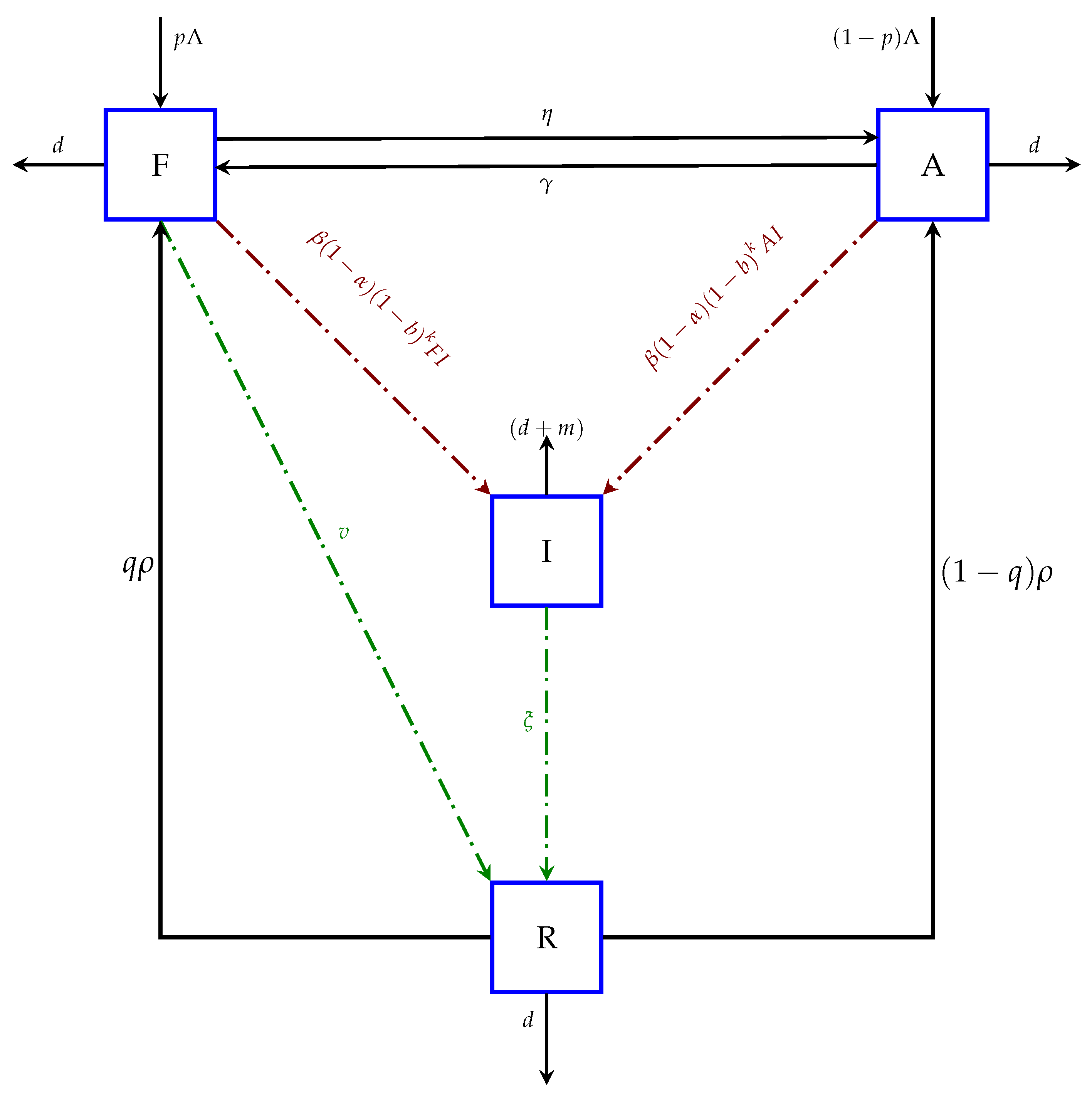
3. Mathematical Model

The work deals with a compartmental SIRS model, where two different susceptible states are considered based on their attitudes toward vaccination. The total population is divided into four sub-classes, named as, pro-vaccine susceptible population $\left(F\right(t\left)\right)$, anti-vaccine susceptible population $\left(A\right(t\left)\right)$, infected class $\left(I\right(t\left)\right)$ and recovered class $\left(R\right(t\left)\right)$, and the way of disease propagation is depicted in Figure 1. The mode of transmission follows mass action law in this model and $\tilde{\beta }$ presents the infection propagation rate from susceptible to infected class. In the midst of an epidemic, various social platforms serve as vital channels for disseminating critical information about disease symptoms, recommended precautions, and available treatments. These platforms include diverse media outlets such as television, radio, and educational campaigns. Individuals are actively encouraged to adopt appropriate protective measures to safeguard their well-being, while governments implement a range of restrictions and limitations based on the severity of the situation. In this context, the societal component $\alpha$ represents the measure of the effectiveness of the governmental intervention, while the parameters b and k indicate the effectiveness of social behavioral dynamics and public reaction, respectively. It is worth noting that these parameters are bounded within the range of 0 to 1, denoted as $0\le \alpha <1,0\le b<1$. Consequently, individuals from both susceptible classes together move to the infected class when they come into contact with infectious individuals and the combined rate of infection is ${\tilde{\beta }}^{\nu }\left(1-\alpha \right){\left(1-b\right)}^k\left(F\left(t\right)+A\left(t\right)\right)I\left(t\right)$ (see, for instance [22,33,34,35]). The recruitment rate is denoted by ${\tilde{\mathsf{\Lambda }}}^{\nu }$, which determines the rate at which new individuals enter the population. A portion p of this recruitment remains in F class and another portion in A class. Additionally, ${\tilde{v}}^{\nu }$ is the rate at which pro-vaccine individuals move to the recovered compartment due to vaccination. Furthermore, it is assumed that the natural mortality rate ${\tilde{d}}^{\nu }$ incorporates each compartment within the system. Additionally, the disease-related mortality rate ${\tilde{m}}^{\nu }$ is specifically considered in the infected class. As part of the model, individuals who are infected with the disease gain immunity at a rate ${\tilde{\xi }}^{\nu }$. This immunity can result from either natural recovery or clinical treatment, enabling it to transmit to the recovered class. However, it is important to consider the assumption of temporary recovery, as an outcome a portion of the individuals in the recovered class becomes susceptible again over time. This transmission from the recovered class to the susceptible class occurs at a rate ${\tilde{\rho }}^{\nu }$: (i) the probability of progressing to the pro-vaccine susceptible class is q, (ii) the probability of progressing to the anti-vaccine susceptible class is $(1-q)$, $0\le q\le 1$. So, the following epidemic model is developed in Caputo formalism:

$$\begin{array}{cc}& {}_0{}^{C}D_t^{\nu }F\left(t\right)=p{\tilde{\mathsf{\Lambda }}}^{\nu }-{\tilde{\beta }}^{\nu }\left(1-\alpha \right){\left(1-b\right)}^{k}F\left(t\right)I\left(t\right)-{\tilde{v}}^{\nu }F\left(t\right)+{\tilde{\gamma }}^{\nu }A\left(t\right)-{\tilde{\eta }}^{\nu }F\left(t\right)+q{\tilde{\rho }}^{\nu }R\left(t\right)-{\tilde{d}}^{\nu }F\left(t\right)\hfill \\ & {}_0{}^{C}D_t^{\nu }A\left(t\right)=(1-p){\tilde{\mathsf{\Lambda }}}^{\nu }-{\tilde{\beta }}^{\nu }\left(1-\alpha \right){\left(1-b\right)}^{k}A\left(t\right)I\left(t\right)-{\tilde{\gamma }}^{\nu }A\left(t\right)+{\tilde{\eta }}^{\nu }F\left(t\right)+(1-q){\tilde{\rho }}^{\nu }R\left(t\right)-{\tilde{d}}^{\nu }A\left(t\right)\hfill \\ & {}_0{}^{C}D_t^{\nu }I\left(t\right)={\tilde{\beta }}^{\nu }\left(1-\alpha \right){\left(1-b\right)}^k\left(F\left(t\right)+A\left(t\right)\right)I\left(t\right)-{\tilde{\xi }}^{\nu }I\left(t\right)-({\tilde{d}}^{\nu }+{\tilde{m}}^{\nu })I\left(t\right)\hfill \\ & {}_0{}^{C}D_t^{\nu }R\left(t\right)={\tilde{v}}^{\nu }F\left(t\right)+{\tilde{\xi }}^{\nu }I\left(t\right)-({\tilde{\rho }}^{\nu }+{\tilde{d}}^{\nu })R\left(t\right)\hfill \end{array}$$

(4)

All parameters containing $\nu$ as power are denoted as ${\tilde{\mathsf{\Lambda }}}^{\nu }=\mathsf{\Lambda },{\tilde{\beta }}^{\nu }=\beta ,{\tilde{v}}^{\nu }=v,{\tilde{\gamma }}^{\nu }=\gamma ,{\tilde{\eta }}^{\nu }=\eta ,{\tilde{\rho }}^{\nu }=\rho ,{\tilde{d}}^{\nu }=d,{\tilde{\xi }}^{\nu }=\xi ,{\tilde{m}}^{\nu }=m$ for sake of simplicity. Therefore, system (4) becomes:

$$\begin{array}{cc}& {}_0{}^{C}D_t^{\nu }F\left(t\right)=p\mathsf{\Lambda }-\beta \left(1-\alpha \right){\left(1-b\right)}^{k}F\left(t\right)I\left(t\right)-vF\left(t\right)+\gamma A\left(t\right)-\eta F\left(t\right)+q\rho R\left(t\right)-dF\left(t\right)\hfill \\ & {}_0{}^{C}D_t^{\nu }A\left(t\right)=(1-p)\mathsf{\Lambda }-\beta \left(1-\alpha \right){\left(1-b\right)}^{k}A\left(t\right)I\left(t\right)-\gamma A\left(t\right)+\eta F\left(t\right)+(1-q)\rho R\left(t\right)-dA\left(t\right)\hfill \\ & {}_0{}^{C}D_t^{\nu }I\left(t\right)=\beta \left(1-\alpha \right){\left(1-b\right)}^k\left(F\left(t\right)+A\left(t\right)\right)I\left(t\right)-\xi I\left(t\right)-(d+m)I\left(t\right)\hfill \\ & {}_0{}^{C}D_t^{\nu }R\left(t\right)=vF\left(t\right)+\xi I\left(t\right)-(\rho +d)R\left(t\right)\hfill \end{array}$$

(5)

The models (5) is associated to positive initial conditions $F\left(0\right)>0$, $A\left(0\right)>0$, $I\left(0\right)>0$ and $R\left(0\right)>0$. The descriptions of the model parameters and variables are presented in

Table 1. Descriptions of system parameters from a biological perspective.

Parameters/Variables	Biological Meaning of the Variables and Parameter
$F\left(t\right)$	For-vaccination susceptible compartment
$A\left(t\right)$	Against-vaccination susceptible compartment
$I\left(t\right)$	Infected compartment
$R\left(t\right)$	Recovered compartment
p	Portion of the recruitment goes in $F\left(t\right)$ class
$(1-p)$	Portion of the recruitment goes in $A\left(t\right)$ class
$\tilde{\mathsf{\Lambda }}$	The recruitment rate
$\tilde{\beta }$	Coefficient of rate of propagation of infection for susceptible classes
$\alpha$	The effectiveness of governmental intervention
b	The effectiveness of social behavioral dynamics
k	Strength of public reaction
$\tilde{v}$	Immunization rate of for-vaccination compartment
$\tilde{\gamma }$	Migration rate from against-vaccination to for-vaccination compartment through awareness
$\tilde{\eta }$	Migration rate from for-vaccination to against-vaccination compartment through receiving false information about vaccines
q	Portion of the recovered goes in $F\left(t\right)$ class
$(1-q)$	Portion of the recovered goes in $A\left(t\right)$ class
$\tilde{\rho }$	Rate of chance of reinfection
$\tilde{d}$	Natural death rate
$\tilde{\xi }$	Recovery rate of infected class
$\tilde{m}$	Disease related mortality rate

.

Note (Description of incidence rate $\beta \left(1-\alpha \right){\left(1-b\right)}^k\left(F\left(t\right)+A\left(t\right)\right)I\left(t\right)$): Here, in this expression $\beta$ is the rate at which an infected person can transmit the infection to the individual of susceptible classes F and A, respectively. Therefore, the incidence rate between the susceptible classes and the infected class appeared as $\beta \left(F\left(t\right)+A\left(t\right)\right)I\left(t\right)$. Now, if we assume that government implements some regulations to prevent disease propagation, then this transmission rate will depend on the strength of governmental intervention ($\alpha$), effectiveness of sociological behavioral dynamics (b) and strength of public reaction (k). Now, the growing intensity of governmental action ($\alpha$) will diminish disease transmission and this effect can be incorporated by multiplying a factor $(1-\alpha )$ by the disease transmission rate. Thus, the individuals will now leave the susceptible class F and A at rate $(1-\alpha )\beta F\left(t\right)I\left(t\right)$ and $(1-\alpha )\beta A\left(t\right)I\left(t\right)$, respectively. If the people are motivated by the measures of government action to prevent transmission of disease, the effectiveness of sociological behavioral dynamics (d) and strength of public reaction (k) will increase and ultimately reduce the spreading of the ailment.

In the proposed system, it is assumed that $0\le \alpha \le 1,0\le b\le 1$. Now, the scenarios $\alpha =0$ and $b=0$ signify that there is an absence of governmental intervention and a lack of social behavioral dynamics, respectively. As these sociological parameters approach the value 1, the factor $(1-\alpha )(1-b)$ reduces. The dynamics of social behavior and the reactions of the public are intricately linked to each other. Now, taking the parameter public reaction $\left(k\right)$ as an exponent applied to $(1-b)$ accelerates the reduction in the term ${(1-b)}^k$. Consequently, the overall factor $(1-\alpha ){(1-b)}^k$ becomes a notably smaller quantity. Thus, when we multiply this factor with the transmission rate $\beta \left(F\right(t)+A(t\left)\right)I\left(t\right)$, the rate at which individuals (from the susceptible classes) move to the infected class can be expressed as $\beta \left(1-\alpha \right){\left(1-b\right)}^k\left(F\left(t\right)+A\left(t\right)\right)I\left(t\right)$. Considering the transmission rate as $\beta \left(1-\alpha \right){\left(1-b\right)}^k\left(F\left(t\right)+A\left(t\right)\right)I\left(t\right)$ signifies that as the amplitude of $\alpha$, b and k rises, the infection rate from susceptible to infected class falls, which is more realistic.

4. Existence and Uniqueness

To establish the existence and uniqueness of the solution for the model (5), the following lemma is required.

Lemma 3

([36]). Consider the system:

$${}_{t_0}{}^{C}D_t^{\nu }y\left(t\right)=f(t,y),t_0>0$$

(6)

with initial condition $y\left(t_0\right)=y_{t_0},$ where $\nu \in (0,1]$, $f:[t_0,\infty )\times \mathcal{T}⟶{\mathbb{R}}^n$, $\mathcal{T}\in {\mathbb{R}}^n$, if $f(t,y)$ satisfies the local Lipschitz condition with respect to y, then there exists a unique solution of (6) on $[t_0,\infty )\times \mathcal{T}$.

To study the existence and uniqueness of the solution of system (5), consider the region $\mathcal{T}\times \left[0,T\right]$ where

$$\mathcal{T}=\left\{\left(F\left(t\right),A\left(t\right),I\left(t\right),R\left(t\right)\right)\in {\mathbb{R}}^4:max\left\{\right|F\left(t\right)|,|A\left(t\right)|,|I\left(t\right)|,|R\left(t\right)|\}\le M\right\}$$

and $T<\infty$. Let us denote $X=\left(F\left(t\right),A\left(t\right),I\left(t\right),R\left(t\right)\right)$ and $\overline{X}=\left(\overline{F}\left(t\right),\overline{A}\left(t\right),\overline{I}\left(t\right),\overline{R}\left(t\right)\right)$. Consider a mapping

$$L\left(X\right)=\left(L_1\left(X\right),L_2\left(X\right),L_3\left(X\right),L_4\left(X\right)\right)$$

where

$$\begin{array}{cc}& L_1\left(X\right)=p\mathsf{\Lambda }-\beta \left(1-\alpha \right){\left(1-b\right)}^{k}F\left(t\right)I\left(t\right)-vF\left(t\right)+\gamma A\left(t\right)-\eta F\left(t\right)+q\rho R\left(t\right)-dF\left(t\right)\hfill \\ & L_2\left(X\right)=(1-p)\mathsf{\Lambda }-\beta \left(1-\alpha \right){\left(1-b\right)}^{k}A\left(t\right)I\left(t\right)-\gamma A\left(t\right)+\eta F\left(t\right)+(1-q)\rho R\left(t\right)-dA\left(t\right)\hfill \\ & L_3\left(X\right)=\beta \left(1-\alpha \right){\left(1-b\right)}^k\left(F\left(t\right)+A\left(t\right)\right)I\left(t\right)-\xi I\left(t\right)-(d+m)I\left(t\right)\hfill \\ & L_4\left(X\right)=vF\left(t\right)+\xi I\left(t\right)-\rho R\left(t\right)-dR\left(t\right)\hfill \end{array}$$

Now,

$$\begin{array}{ccc}\hfill \parallel L\left(X\right)-L\left(\overline{X}\right)\parallel & =& |L_1\left(X\right)-L_1\left(\overline{X}\right)|+|L_2\left(X\right)-L_2\left(\overline{X}\right)|+|L_3\left(X\right)-L_3\left(\overline{X}\right)|+|L_4\left(X\right)-L_4\left(\overline{X}\right)|\hfill \\ \hfill & =& {|-\beta (1-\alpha )(1-b)}^k\left(FI-\overline{F}\overline{I}\right)-v(F-\overline{F})+\gamma (A-\overline{A})\hfill \\ \hfill & & -\eta (F\left(t\right)-\overline{F})+q\rho (R-\overline{R})-d(F-\overline{F})|+|-\beta (1-\alpha ){(1-b)}^k\hfill \\ \hfill & & \left(AI-\overline{A}\overline{I}\right)-(\gamma +d)(A-\overline{A})+\eta (F-\overline{F})\hfill \\ \hfill & & +(1-q)\rho (R\left(t\right)-\overline{R}\left(t\right)){|+|\beta (1-\alpha )(1-b)}^k\{\left(F+A\right)I-\left(\overline{F}\right.\hfill \\ \hfill & & \left.+\overline{A}\right)\overline{I}\}-(\xi +d+m)(I-\overline{I})|+|v(F-\overline{F})+\xi (I-\overline{I})\hfill \\ \hfill & & -(\xi +d)(R-\overline{R})|\hfill \\ & \le & \beta (1-\alpha ){(1-b)}^k|FI-\overline{F}\overline{I}|+(v+\eta +d)|F-\overline{F}|+\gamma |A-\overline{A}|+q\rho |R-\overline{R}|\hfill \\ & & +\beta (1-\alpha ){(1-b)}^k|AI-\overline{A}\overline{I}|+(\gamma +d)|A-\overline{A}|+\eta |F-\overline{F}|+(1-q)\rho |R-\overline{R}|\hfill \\ & & +\beta (1-\alpha ){(1-b)}^k|(F+A)I-(\overline{F}+\overline{A})\overline{I}|+(\xi +d+m)|I-\overline{I}|+v|F-\overline{F}|\hfill \\ & & +\xi |I-\overline{I}|+(\rho +d)|R-\overline{R}|\hfill \\ & \le & \left(2M\beta (1-\alpha ){(1-b)}^k+2v+2\eta +d\right)|F-\overline{F}|+\left(2M\beta (1-\alpha ){(1-b)}^k+2\gamma \right.\hfill \\ & & \left.+d\right)|A-\overline{A}|+\left(4M\beta (1-\alpha ){(1-b)}^k+2\xi +d+m\right)|I-\overline{I}|+(\rho +\xi +d)|R-\overline{R}|\hfill \end{array}$$

Let

$$\begin{array}{ccc}\hfill E& =& max\{\left[2M\beta (1-\alpha ){(1-b)}^k+2v+2\eta +d\right],\left[2M\beta (1-\alpha ){(1-b)}^k+2\gamma +d\right],\hfill \\ & & \left[4M\beta (1-\alpha ){(1-b)}^k+2\xi +d+m\right],(\rho +\xi +d)\}\hfill \end{array}$$

$$\therefore \parallel L\left(X\right)-L\left(\overline{X}\right)\parallel \le E\parallel X-\overline{X}\parallel$$

Thus, $L\left(X\right)$ satisfies the Lipschitz’s condition with respect to X, it follows from Lemma that there exists a unique solution $X\left(t\right)$ of the system (5) with initial condition $X\left(0\right)=(F_0,A_0,I_0,R_0)$.

This result holds true within the domain $\mathcal{T}$, indicating that we can obtain the same outcome in the context of the population dynamics model, specifically in $0\le F\left(t\right),A\left(t\right),I\left(t\right),$$R\left(t\right)<\delta$ which is a subset of ${\mathbb{R}}^4$ [37]. Next, our aim is to prove the following Lemma 4.

Lemma 4.

All the solutions of system (5) which start in ${\mathbb{R}}_{+}^4$ and satisfy $0\le F\left(t\right),A\left(t\right),I\left(t\right),$$R\left(t\right)<\delta$, $t\in [0,\infty )$ are embedded in the region Θ, where

$$\Theta =\left\{\left(F,A,I,R\right)\in {\mathbb{R}}_{+}^4:F+A+I+R<{\displaystyle \frac{\mathsf{\Lambda }}{d}}+\epsilon ,\epsilon >0\right\}.$$

Proof. 

Let $\mathsf{\Omega }\left(t\right)=F\left(t\right)+A\left(t\right)+I\left(t\right)+R\left(t\right)$. Taking the fractional derivative of order $\nu$, we obtain

$$\begin{array}{ccc}\hfill {}_0{}^{C}D_t^{\nu }\mathsf{\Omega }& =& {}_0{}^{C}D_t^{\nu }\left(F\left(t\right)+A\left(t\right)+I\left(t\right)+R\left(t\right)\right)\hfill \\ & =& \mathsf{\Lambda }-d\left(F\left(t\right)+A\left(t\right)+I\left(t\right)+R\left(t\right)\right)-mI\left(t\right)\hfill \\ & \le & \mathsf{\Lambda }-d\mathsf{\Omega }\left(t\right)\hfill \end{array}$$

Using the Lemma 1, we have

$$\begin{array}{c}\hfill \mathsf{\Omega }\left(t\right)\le \left(\mathsf{\Omega }\left(0\right)-{\displaystyle \frac{\mathsf{\Lambda }}{d}}\right)E_{\nu }\left[-d{t}^{\nu }\right]+{\displaystyle \frac{\mathsf{\Lambda }}{d}}\end{array}$$

Due to the positiveness of the Mittag–Leffler function $E_{\nu }$ and taking the limit $t\to \infty$, we obtain from the above inequality:

$$\underset{t⟶\infty }{lim\; sup}\mathsf{\Omega }\left(t\right)\le {\displaystyle \frac{\mathsf{\Lambda }}{d}}+\epsilon$$

for some positive real number $\epsilon$. Therefore, all the solutions of the system (5) are embedded in the region:

$$\Theta =\left\{(F,A,I,R)\in {\mathbb{R}}_{+}^4:F+A+I+R<{\displaystyle \frac{\mathsf{\Lambda }}{d}}+\epsilon ,\epsilon >0\right\}.$$

 □

5. Equilibrium Points and Stability Analysis

Definition 3

([36]). A constant $y^{\ast }$ is an equilibrium point of the Caputo fractional dynamic system (6), if and only if $f(t,y^{\ast })=0$.

Therefore, the equilibrium points of the system (5) can be obtained by solving the following equations:

$$\begin{array}{ccc}\hfill \hspace{0.17em}& & p\mathsf{\Lambda }-\beta \left(1-\alpha \right){\left(1-b\right)}^{k}F\left(t\right)I\left(t\right)-vF\left(t\right)+\gamma A\left(t\right)-\eta F\left(t\right)+q\rho R\left(t\right)-dF\left(t\right)=0,\hfill \\ & & (1-p)\mathsf{\Lambda }-\beta \left(1-\alpha \right){\left(1-b\right)}^{k}A\left(t\right)I\left(t\right)-\gamma A\left(t\right)+\eta F\left(t\right)+(1-q)\rho R\left(t\right)-dA\left(t\right)=0,\hfill \\ \hfill & & \beta \left(1-\alpha \right){\left(1-b\right)}^k\left(F\left(t\right)+A\left(t\right)\right)I\left(t\right)-\xi I\left(t\right)-(d+m)I\left(t\right)=0,\hfill \\ \hfill & & vF\left(t\right)+\xi I\left(t\right)-(\rho +d)R\left(t\right)=0.\hfill \end{array}$$

(7)

Solving these equations, we have the following equilibrium points, namely

• Disease free equilibrium point (DFE), $E_f(F_1,A_1,0,R_1)$:
  Here, $F_1={\displaystyle \frac{\mathsf{\Lambda }(\rho +d)(pd+\gamma )}{d\left[(v+\rho +d)(d+\gamma )+(\rho +d)\eta +(1-q)\rho v\right]}}$, $A_1={\displaystyle \frac{\mathsf{\Lambda }\left[(v+\rho +d)(1-p)d+(\rho +d)\eta +(1-q)\rho v\right]}{d\left[(v+\rho +d)(d+\gamma )+(\rho +d)\eta +(1-q)\rho v\right]}}$,
  $R_1={\displaystyle \frac{\mathsf{\Lambda }(pd+\gamma )v}{d\left[(v+\rho +d)(d+\gamma )+(\rho +d)\eta +(1-q)\rho v\right]}}.$
  The basic reproduction number $\left(R_0\right)$ represents the number of newly infected people from a single infected individual in a susceptible environment. The procedure developed by van den Driessche and Watmough is usually used to obtain $R_0$ [38]. Let, $z\equiv (I,R)$. Then we have: ${\displaystyle \frac{dz}{dt}=\Phi \left(z\right)-\Psi \left(z\right),}$ where

  $$\Phi \left(z\right)=\left(\begin{array}{c}\beta \left(1-\alpha \right){\left(1-b\right)}^k\left(F+A\right)I\\ 0\end{array}\right)\mathrm{and}\Psi \left(z\right)=\left(\begin{array}{c}(\xi +d+m)I\\ -vF-\xi I+(\rho +d)R\end{array}\right).$$
  Here, $\Phi \left(z\right)$ and $\Psi \left(z\right)$ contain the compartment with the new infection term and the rest of the terms, respectively. Then, at $E_f(F_1,A_1,0,R_1)$, we have

  $${\displaystyle \widehat{\Phi }={\left(D\Phi \left(z\right)\right)}_{E_f}=\left(\begin{array}{cc}\beta \left(1-\alpha \right){\left(1-b\right)}^k\left(F_1+A_1\right)& 0\\ 0& 0\end{array}\right)}$$

  $$\mathrm{and}\widehat{\Psi }={\left(D\Psi \left(z\right)\right)}_{E_f}=\left(\begin{array}{cc}(\xi +d+m)& 0\\ -\xi & (\rho +d)\end{array}\right).$$
  Now, $R_0$ is the spectral radius of the next generation matrix $\widehat{\Phi }{\widehat{\Psi }}^{-1}$ and is denoted by:

  $$\begin{array}{cc}\hfill R_0& ={\displaystyle \frac{\beta (1-\alpha ){(1-b)}^k(F_1+A_1)}{(\xi +d+m)}}\hfill \\ \hfill & ={\displaystyle \frac{\mathsf{\Lambda }\beta (1-\alpha ){(1-b)}^k}{d(\xi +d+m)}}\left[{\displaystyle \frac{(\rho +d)(d+\gamma +\eta )+(1-p)vd+(1-q)\rho v}{(\rho +d)(d+\gamma +\eta )+v(d+\gamma )+(1-q)\rho v}}\right].\hfill \end{array}$$

  (8)

Remark 1.

It is important to note that the basic reproduction number $R_0$ appears to be independent of ν, the order of the fractional derivative. However, it indirectly depends on ν because many of the parameters involved in the expression of $R_0$ are functions of ν.

• Interior equilibrium point, $E^{\ast }(F^{\ast },A^{\ast },I^{\ast },R^{\ast })$:
  $F^{\ast }={\displaystyle \frac{(\rho +d)\left[\mathsf{\Lambda }{k}_1-k_{2}d+k_1(\xi -k_2)I^{\ast }\right]-\xi d{k}_1{I}^{\ast }}{v{k}_{1}d}}$, $A^{\ast }={\displaystyle \frac{v{k}_{2}d-(\rho +d)\left[\mathsf{\Lambda }{k}_1-k_{2}d+k_1(\xi -k_2)I^{\ast }\right]+\xi d{k}_1{I}^{\ast }}{v{k}_{1}d}}$,
  $R^{\ast }={\displaystyle \frac{\mathsf{\Lambda }{k}_1-k_{2}d+k_1(\xi -k_2)I^{\ast }}{d{k}_1}}$ and $I^{\ast }$ is the positive root of the given equation:

  $$a_0{x}^2+a_{1}x+a_2=0$$

  (9)
  $$\begin{array}{ccc}\hfill a_0& =& k_1^2\left[(d+m)(\rho +d)+\xi d\right],\hfill \\ \hfill a_1& =& k_1\left[2d\left(\rho +d)+d(v+\eta +\gamma \right)k_2+(d+m)\left((1-q)v+\gamma +\eta \right)-d\xi \rho -k_1\mathsf{\Lambda }(\rho +d)\right],\hfill \\ \hfill a_2& =& d{k}_2\left[(\rho +d)(\gamma +\eta +d)+(d+\gamma )v+(1-q)\rho v\right](1-R_0),\hfill \\ \hfill k_2& =& (\xi +m+d),\hfill \\ \hfill k_1& =& \beta (1-\alpha ){(1-b)}^k,\hfill \end{array}$$

  provided $v{k}_{2}d>(\rho +d)\left[\mathsf{\Lambda }{k}_1-k_{2}d+k_1(\xi -k_2)I^{\ast }\right]>\xi d{k}_1{I}^{\ast }$. Table 2 provides an overview of possible positive roots of the Equation (9).

Table 2. Number of possible positive roots of Equation (9).

Reproduction Number	Sign of Coefficients of (9)			Number of Positive Roots
$R_0<1$	$a_0>0$	$a_1>0$	$a_2>0$	0
	$a_0>0$	$a_1<0$	$a_2>0$	2 (if $a_1^2-4a_0{a}_2\ge 0$) 0 (if $a_1^2-4a_0{a}_2<0$)
$R_0=1$	$a_0>0$	$a_1>0$	$a_2=0$	0
	$a_0>0$	$a_1<0$	$a_2=0$	1
$R_0>1$	$a_0>0$	$a_1>0$	$a_2<0$	1
	$a_0>0$	$a_1<0$	$a_2<0$	1

Table 2. Number of possible positive roots of Equation (9).

Reproduction Number	Sign of Coefficients of (9)			Number of Positive Roots
$R_0<1$	$a_0>0$	$a_1>0$	$a_2>0$	0
	$a_0>0$	$a_1<0$	$a_2>0$	2 (if $a_1^2-4a_0{a}_2\ge 0$) 0 (if $a_1^2-4a_0{a}_2<0$)
$R_0=1$	$a_0>0$	$a_1>0$	$a_2=0$	0
	$a_0>0$	$a_1<0$	$a_2=0$	1
$R_0>1$	$a_0>0$	$a_1>0$	$a_2<0$	1
	$a_0>0$	$a_1<0$	$a_2<0$	1

Local Stability Analysis

Theorem 2.

The disease-free equilibrium point $E_f(F_1,A_1,0,R_1)$ is locally asymptotically stable if $R_0<1$.

Proof. 

The Jacobian matrix corresponding to the disease-free equilibrium point $E_f(F_1,A_1,0,$ $R_1)$ is given by

$$J_1\left(F_1,A_1,0,R_1\right)=\left[\begin{array}{cccc}-(v+\eta +d)& \gamma & -\beta (1-\alpha ){(1-b)}^k{F}_1& q\rho \\ \eta & -(\gamma +d)& -\beta (1-\alpha ){(1-b)}^k{A}_1& (1-q)\rho \\ 0& 0& \beta (1-\alpha ){(1-b)}^k(F_1+A_1)-(\xi +d+m)& 0\\ v& 0& \xi & -(\rho +d)\end{array}\right],$$

The characteristic equation of $J_1\left(F_1,A_1,0,R_1\right)$ is

$$\begin{array}{c}\hfill (d+\lambda )\left\{\lambda -\beta (1-\alpha ){(1-b)}^k(F_1+A_1)+(\xi +d+m)\right\}\{{\lambda }^2+(2d+v+\gamma +\eta +\rho )\lambda \\ \hfill +d^2+dv+d\gamma +v\gamma +d\eta +d\rho +(1-q)v\rho +\gamma \rho +\eta \rho \}=0\end{array}$$

Therefore, all the eigenvalues are given by ${\lambda }_1=-d$, ${\lambda }_2=\beta (1-\alpha ){(1-b)}^k(F_1+A_1)-(\xi +d+m)$ and

$${\lambda }_{3,4}={\displaystyle \frac{-(2d+v+\gamma +\eta +\rho )\pm \sqrt{{(2d+v+\gamma +\eta +\rho )}^2-4\{(d+\gamma )(d+\rho +v)+\eta (d+\rho )+(1-q)\rho v\}}}{2}}.$$

Now, if ${(2d+v+\gamma +\eta +\rho )}^2-4\{(d+\gamma )(d+\rho +v)+\eta (d+\rho )+(1-q)\rho v\}\ge 0$, eigenvalues ${\lambda }_i$, $i=3,4$ are real and negative but if ${(2d+v+\gamma +\eta +\rho )}^2-4\{(d+\gamma )(d+\rho +v)+\eta (d+\rho )+(1-q)\rho v\}<0$, ${\lambda }_i$, $i=3,4$ are complex and lie in the left-half complex plane (stable region as depicted in Figure 2), i.e, in all possible cases $|arg{\lambda }_{3,4}|>{\displaystyle \frac{\nu \pi }{2}}$, $\nu \in (0,1)$ [39]. Again, if $\beta (1-\alpha ){(1-b)}^k(F_1+A_1)-(\xi +d+m)<0$, i.e., $R_0<1$, then ${\lambda }_2<0$. Thus, $\left|arg\left({\lambda }_i\right)\right|>{\displaystyle \frac{\nu \pi }{2}}$, for $i=1,2,3,4$ if $R_0<1$. Hence, by Proposition 1, the disease free equilibrium point, $E_f(F_1,A_1,0,R_1)$ is locally asymptotically stable if $R_0<1$.  □

Lemma 5

([39]). Let $D\left(P\right)$ be the discriminant of the characteristic polynomial $P\left(\lambda \right)={\lambda }^4+p_1{\lambda }^3+p_2{\lambda }^2+p_3\lambda +p_4$ of the Jacobian matrix corresponding to an equilibrium point, where $D\left(P\right)$ is given by

$$D\left(P\right)=\left[\begin{array}{ccccccc}1& p_1& p_2& p_3& p_4& 0& 0\\ 0& 1& p_1& p_2& p_3& p_4& 0\\ 0& 0& 1& p_1& p_2& p_3& p_4\\ 4& 3p_1& 2p_2& p_3& 0& 0& 0\\ 0& 0& 4& 3p_1& 2p_2& p_3& 0\\ 0& 0& 0& 4& 3p_1& 2p_2& p_3\end{array}\right].$$

Then, the following propositions hold:

1. 

If ${\mathsf{\Delta }}_1$, ${\mathsf{\Delta }}_2$, ${\mathsf{\Delta }}_3$ and ${\mathsf{\Delta }}_4$ are Routh–Hurwitz determinants

$${\mathsf{\Delta }}_1=p_1,{\mathsf{\Delta }}_2=\left|\begin{array}{cc}{p}_1& 1\\ p_3& p_2\end{array}\right|,{\mathsf{\Delta }}_3=\left|\begin{array}{ccc}{p}_1& 1& 0\\ p_3& p_2& p_1\\ 0& p_4& p_3\end{array}\right|,{\mathsf{\Delta }}_4=\left|\begin{array}{cccc}{p}_1& 1& 0& 0\\ p_3& p_2& p_1& 1\\ 0& p_4& p_3& p_2\\ 0& 0& 0& p_4\end{array}\right|,$$

then for $\nu =1$, the necessary and sufficient conditions for the interior equilibrium point $E^{\ast }$ to be locally asymptotically stable are

$${\mathsf{\Delta }}_1>0,{\mathsf{\Delta }}_2>0,{\mathsf{\Delta }}_3>0\mathrm{and}{\mathrm{p}}_4>0$$

2. 

If $D\left(P\right)>0$, $p_1>0$, $p_2<0$ and $\nu >{\displaystyle \frac{2}{3}}$, then $E^{\ast }$ is unstable.

3. 

If $D\left(P\right)<0$, $p_1>0$, $p_2>0$, $p_3>0$, $p_4>0$ and $\nu <{\displaystyle \frac{1}{3}}$, then $E^{\ast }$ is locally asymptotically stable. Also, if $D\left(P\right)<0$, $p_1<0$, $p_2>0$, $p_3<0$, $p_4>0$, then $E^{\ast }$ is unstable.

4. 

If $D\left(P\right)<0$, $p_1>0$, $p_2>0$, $p_3>0$, $p_4>0$ and $p_2={\displaystyle \frac{p_1{p}_4}{p_3}}+{\displaystyle \frac{p_3}{p_1}}$, then the equilibrium point $E^{\ast }$ is locally asymptotically stable, for all $\nu \in (0,1)$.

5. 

$p_4>0$ is the necessary condition for the equilibrium point $E^{\ast }$ to be locally asymptotically stable.

Theorem 3.

The coexistence equilibrium point $E^{\ast }(F^{\ast },A^{\ast },I^{\ast },R^{\ast })$ is locally asymptotically stable

1. 

for $\nu \in (0,{\displaystyle \frac{1}{3}})$, if $D\left(P\right)<0$,

2. 

for $\nu \in (0,1)$, if $D\left(P\right)<0$ and $p_2={\displaystyle \frac{p_1{p}_4}{p_3}}+{\displaystyle \frac{p_3}{p_1}}$,

3. 

for $\nu =1$, if ${\mathsf{\Delta }}_1>0,{\mathsf{\Delta }}_2>0,{\mathsf{\Delta }}_3>0$ and $p_4>0$.

Proof. 

The Jacobian matrix corresponding to the disease-free equilibrium point, $E^{\ast }(F^{\ast },A^{\ast },$$I^{\ast },R^{\ast })$ is given by

$$J_1\left(F^{\ast },A^{\ast },I^{\ast },R^{\ast }\right)=\left[\begin{array}{cccc}-(d+v+\eta +k_1{I}^{\ast })& \gamma & -k_1{F}^{\ast }& q\rho \\ \eta & -(\gamma +d+k_1{I}^{\ast })& -k_1{A}^{\ast }& (1-q)\rho \\ k_1{I}^{\ast }& k_1{I}^{\ast }& 0& 0\\ v& 0& \xi & -(\rho +d)\end{array}\right].$$

The characteristic equation of $J\left(E^{\ast }\right)$ is

$${\lambda }^4+p_1{\lambda }^3+p_2{\lambda }^2+p_3\lambda +p_4=0,$$

where

$$\begin{array}{ccc}\hfill p_1& =& 3d+v+\gamma +\eta +\rho +2k_1{I}^{\ast },\hfill \\ \hfill p_2& =& 3d^2+v\gamma +\rho ((1-q)v+\gamma +\eta )+2d(v+\gamma +\eta +\rho )+k_1{I}^{\ast }\{4d+v+\gamma +\eta +2\rho +k_1{I}^{\ast }\hfill \\ & & +(\xi +m+d)\},\hfill \\ \hfill p_3& =& d^2(d+v+\gamma +\eta +\rho )+d((1-q)v+\gamma +\eta )+dv\gamma +k_1{I}^{\ast }\left[d(2d+v+\gamma +\eta )+\rho (2d\right.\hfill \\ & & \left.+(1-q)v+\gamma +\eta )+k_1{I}^{\ast }(d+\rho )+(2d+\gamma +\eta +k_1{I}^{\ast })(\xi +m+d)+\rho (m+d)\right],\hfill \\ \hfill p_4& =& k_1{I}^{\ast }\left[d(m+d+\xi )(d+\gamma +\eta +k_1{I}^{\ast })+\rho (m+d)(d+(1-q)v+\gamma +\eta +k_1{I}^{\ast })+k_{1}vd{A}^{\ast }\right].\hfill \end{array}$$

From the above expressions, it is clear that $p_i>0$, for $i=1,2,3,4.$ Therefore, using Lemma 5, we have, $E^{\ast }$ is locally asymptotically stable for

• $\nu <{\displaystyle \frac{1}{3}}$, if $D\left(P\right)<0$.
• all $\nu \in (0,1)$, if $D\left(P\right)<0$ and $p_2={\displaystyle \frac{p_1{p}_4}{p_3}}+{\displaystyle \frac{p_3}{p_1}}.$
• $\nu =1$, if ${\mathsf{\Delta }}_1>0,{\mathsf{\Delta }}_2>0,{\mathsf{\Delta }}_3>0$ and $p_4>0$.

 □

Remark 2.

In this model, the underlying assumption is that the recovery from infection is not enduring. The immunity acquired by individuals who have recovered may gradually diminish, eventually causing them to transition back into a susceptible state after a certain period of time has elapsed. Therefore, the infection-free steady state or endemic state may not exhibit global stability under any specific parametric condition. Consequently, our analysis focuses solely on the local stability of the equilibrium points in this context.

In Figure 3, we have illustrated the population sizes at a steady state for changing the reproduction number. It becomes evident that when the reproduction number ($R_0$) is below 1, there are no infected individuals; however, once it surpasses the threshold 1, the entire population is present. Consequently, the system remains disease-free when $R_0$ is less than 1, but it becomes endemic when $R_0$ exceeds 1.

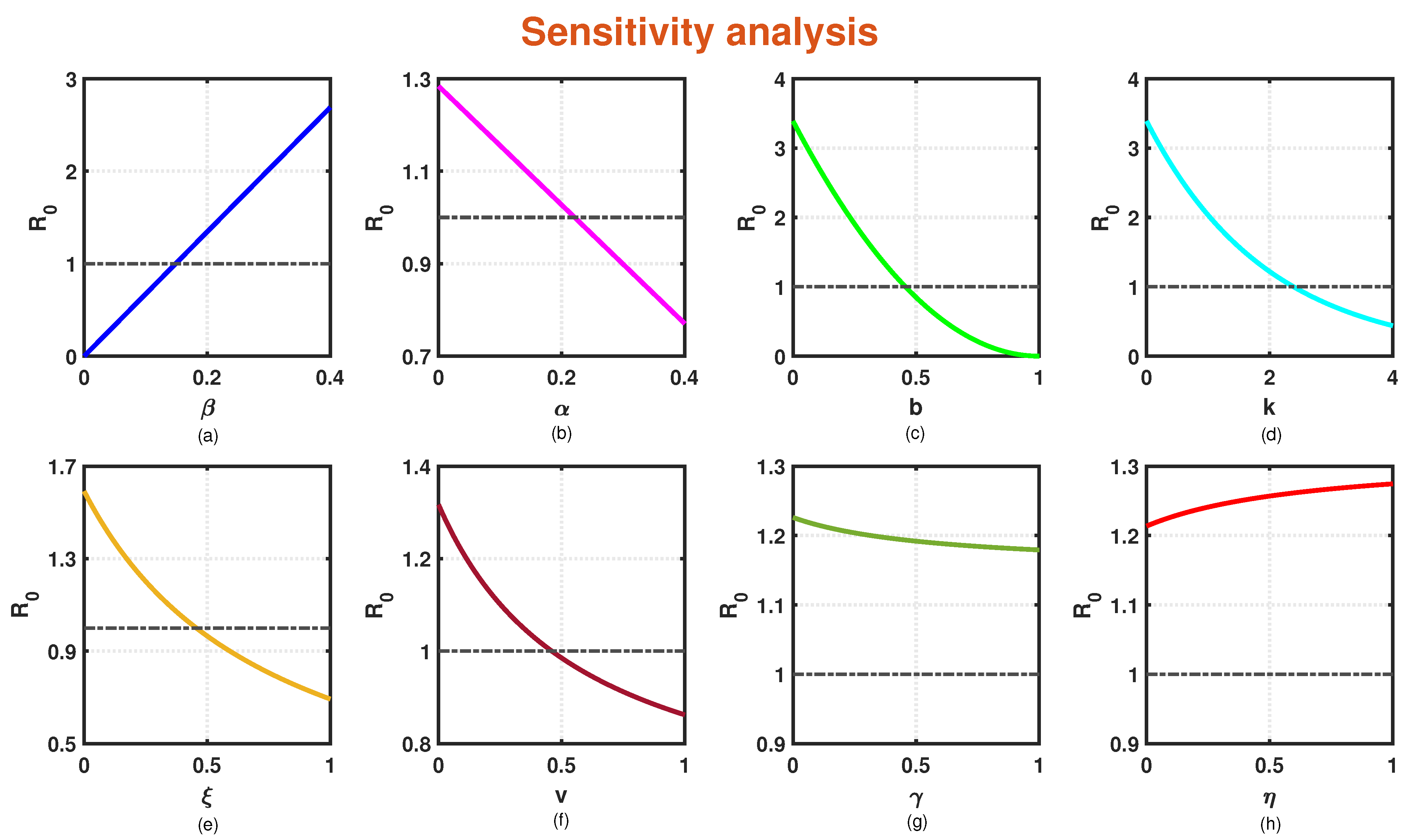
6. Sensitivity Analysis

The basic reproduction number $R_0$ depends on the parameters of the model. Consequently, conducting an analysis to examine the implications of these system parameters on disease propagation is significantly important. The basic reproduction number for (5) is

$$\begin{array}{cc}\hfill R_0& ={\displaystyle \frac{\beta (1-\alpha ){(1-b)}^k(F_1+A_1)}{(\xi +d+m)}}\hfill \\ \hfill & ={\displaystyle \frac{\mathsf{\Lambda }\beta (1-\alpha ){(1-b)}^k}{d(\xi +d+m)}}\left[{\displaystyle \frac{(\rho +d)(d+\gamma +\eta )+(1-p)vd+(1-q)\rho v}{(\rho +d)(d+\gamma +\eta )+v(d+\gamma )+(1-q)\rho v}}\right].\hfill \end{array}$$

where $F_1={\displaystyle \frac{\mathsf{\Lambda }(\rho +d)(pd+\gamma )}{d\left[(v+\rho +d)(d+\gamma )+(\rho +d)\eta +(1-q)\rho v\right]}}$, $A_1={\displaystyle \frac{\mathsf{\Lambda }\left[(v+\rho +d)(1-p)d+(\rho +d)\eta +(1-q)\rho v\right]}{d\left[(v+\rho +d)(d+\gamma )+(\rho +d)\eta +(1-q)\rho v\right]}}$. Hence we have as follows:

$$\begin{array}{cc}\hfill {\displaystyle \frac{\partial R_0}{\partial \beta }}=& {\displaystyle \frac{(1-\alpha ){(1-b)}^k(F_1+A_1)}{(\xi +d+m)}}>0,{\displaystyle \frac{\partial R_0}{\partial \alpha }}=-{\displaystyle \frac{\beta {(1-b)}^k(F_1+A_1)}{(\xi +d+m)}}<0\hfill \\ \hfill {\displaystyle \frac{\partial R_0}{\partial b}}=& -{\displaystyle \frac{k\beta (1-\alpha ){(1-b)}^{k-1}(F_1+A_1)}{(\xi +d+m)}}<0,{\displaystyle \frac{\partial R_0}{\partial k}}={\displaystyle \frac{\beta (1-\alpha ){(1-b)}^k(F_1+A_1)ln(1-b)}{(\xi +d+m)}}<0\hfill \\ \hfill {\displaystyle \frac{\partial R_0}{\partial \xi }}=& -{\displaystyle \frac{\beta (1-\alpha ){(1-b)}^k(F_1+A_1)}{{(\xi +d+m)}^2}}<0\hfill \\ \hfill {\displaystyle \frac{\partial R_0}{\partial v}}=& -{\displaystyle \frac{\mathsf{\Lambda }\beta (1-\alpha ){(1-b)}^k}{d(\xi +d+m)}}{\displaystyle \frac{(\rho +d)(d+\gamma +\eta )(\rho d+\gamma )}{{\left[(\rho +d)(d+\gamma +\eta )+v(d+\gamma )+(1-q)\rho v\right]}^2}}<0\hfill \\ \hfill {\displaystyle \frac{\partial R_0}{\partial \gamma }}=& -{\displaystyle \frac{\mathsf{\Lambda }\beta (1-\alpha ){(1-b)}^k}{d(\xi +d+m)}}{\displaystyle \frac{\left[\left\{(1-p)d+\eta \right\}(\rho +d)+(1-p)vd+(1-q)\rho v\right]}{{\left[(\rho +d)(d+\gamma +\eta )+v(d+\gamma )+(1-q)\rho v\right]}^2}}<0\hfill \\ \hfill {\displaystyle \frac{\partial R_0}{\partial \eta }}=& {\displaystyle \frac{\mathsf{\Lambda }\beta (1-\alpha ){(1-b)}^k}{d(\xi +d+m)}}{\displaystyle \frac{v(\rho +d)(pd+\gamma )}{{\left[(\rho +d)(d+\gamma +\eta )+v(d+\gamma )+(1-q)\rho v\right]}^2}}>0\hfill \end{array}$$

The normalized forward sensitivity indices for the system parameters are provided as follows:

$$\begin{array}{cc}\hfill {\mathsf{{\rm Y}}}_{\beta }=& \left[{\displaystyle \frac{\frac{\partial R_0}{R_0}}{\frac{\partial \beta }{\beta }}}\right]=\left[{\displaystyle \frac{\beta }{R_0}}{\displaystyle \frac{\partial R_0}{\partial \beta }}\right]=1,{\mathsf{{\rm Y}}}_{\alpha }=\left[{\displaystyle \frac{\frac{\partial R_0}{R_0}}{\frac{\partial \alpha }{\alpha }}}\right]=\left[{\displaystyle \frac{\alpha }{R_0}}{\displaystyle \frac{\partial R_0}{\partial \alpha }}\right]=-\left({\displaystyle \frac{\alpha }{1-\alpha }}\right),\hfill \\ \hfill {\mathsf{{\rm Y}}}_b=& \left[{\displaystyle \frac{\frac{\partial R_0}{R_0}}{\frac{\partial b}{b}}}\right]=\left[{\displaystyle \frac{b}{R_0}}{\displaystyle \frac{\partial R_0}{\partial b}}\right]=-k\left({\displaystyle \frac{b}{1-b}}\right),{\mathsf{{\rm Y}}}_k=\left[{\displaystyle \frac{\frac{\partial R_0}{R_0}}{\frac{\partial k}{k}}}\right]=\left[{\displaystyle \frac{k}{R_0}}{\displaystyle \frac{\partial R_0}{\partial k}}\right]=kln(1-b),\hfill \\ \hfill {\mathsf{{\rm Y}}}_{\xi }=& \left[{\displaystyle \frac{\frac{\partial R_0}{R_0}}{\frac{\partial \xi }{\xi }}}\right]=\left[{\displaystyle \frac{\xi }{R_0}}{\displaystyle \frac{\partial R_0}{\partial \xi }}\right]=-{\displaystyle \frac{\xi }{\xi +d+m}},\hfill \\ \hfill {\mathsf{{\rm Y}}}_v=& \left[{\displaystyle \frac{\frac{\partial R_0}{R_0}}{\frac{\partial v}{v}}}\right]=\left[{\displaystyle \frac{v}{R_0}}{\displaystyle \frac{\partial R_0}{\partial v}}\right]=-{\displaystyle \frac{\mathsf{\Lambda }v(\rho +d)(d+\gamma +\eta )(\rho d+\gamma )}{d{\left[(\rho +d)(d+\gamma +\eta )+v(d+\gamma )+(1-q)\rho v\right]}^2(F_1+A_1)}},\hfill \\ \hfill {\mathsf{{\rm Y}}}_{\gamma }=& \left[{\displaystyle \frac{\frac{\partial R_0}{R_0}}{\frac{\partial \gamma }{\gamma }}}\right]=\left[{\displaystyle \frac{\gamma }{R_0}}{\displaystyle \frac{\partial R_0}{\partial \gamma }}\right]=-{\displaystyle \frac{\mathsf{\Lambda }\gamma \left[\left\{(1-p)d+\eta \right\}(\rho +d)+(1-p)vd+(1-q)\rho v\right]}{d{\left[(\rho +d)(d+\gamma +\eta )+v(d+\gamma )+(1-q)\rho v\right]}^2(F_1+A_1)}},\hfill \\ \hfill {\mathsf{{\rm Y}}}_{\eta }=& \left[{\displaystyle \frac{\frac{\partial R_0}{R_0}}{\frac{\partial \eta }{\eta }}}\right]=\left[{\displaystyle \frac{\eta }{R_0}}{\displaystyle \frac{\partial R_0}{\partial \eta }}\right]={\displaystyle \frac{\mathsf{\Lambda }\eta v(\rho +d)(pd+\gamma )}{d{\left[(\rho +d)(d+\gamma +\eta )+v(d+\gamma )+(1-q)\rho v\right]}^2(F_1+A_1)}}.\hfill \end{array}$$

The analysis reveals a significant finding that the coefficient of disease transmission rate $\left(\beta \right)$ exhibits a direct proportional relationship with $R_0$. This observation is particularly relevant, as it implies that a higher contact rate increases the likelihood of individuals becoming infected. Consequently, such circumstances contribute to the establishment of an endemic system characterized by a high prevalence of the disease. However, it is worth noting that effective governmental actions play a crucial role in mitigating the epidemic situation. By imposing strict control measures and interventions, the spread of the disease can be controlled over time. When individuals choose to adopt changes in their social behavior to protect themselves from infection, it serves as an important factor in curbing the spread of disease over time. By implementing preventive measures and adhering to necessary precautions, such as practicing good hygiene, maintaining physical distancing, and wearing masks, the rate of disease propagation can be effectively reduced. Similarly, if individuals respond promptly to the necessary precautionary measures during periods of high disease prevalence, the accelerated rate of transmission can be diminished. It is worth noting that a higher recovery rate plays a vital role in reducing the number of infected individuals within a system. As a larger portion of the infected population recovers, whether through the development of natural immunity or through effective pharmaceutical therapies, the overall infection fatality rate is controlled and diminished over time. Additionally, the vaccination rate $\left(v\right)$ demonstrates an inverse relationship with $R_0$. This relationship provides biological significance since a higher vaccination rate reduces the chances of individuals becoming infected. By providing vaccines to susceptible individuals and those in asymptomatic stages, the likelihood of disease transmission is significantly reduced. The sensitivity index analysis reveals that an increase in awareness levels is associated with a decrease in the population of infected individuals. This can be attributed to the fact that higher awareness levels result in a greater number of individuals being pro-vaccine. As a result, there is an increase in the number of vaccinated individuals, leading to a decrease in the population of infected individuals. This promotes vaccination as an effective strategy in reducing the spread of infectious diseases and protecting public health.

7. Optimal Control

In classical and fractional calculus, the Pontryagin optimal control principle is an extremely important technique [40,41]. For fractional calculus, the approach is identical to that used to resolve the classical integer-order optimal control problem. Certain control issues have been explored previously by employing the Pontryagin principle in the context of fractional-order systems [42,43]. The primary difference lies in the fact that in a fractional-order optimal control problem, the adjoint equations are expressed using the Right-Riemann–Liouville derivative (${}_{t\hspace{1em}}{}^{RL}D_{T_f}^{\nu }$) of order $\nu$ while the co-state equations are formulated as Caputo differential equations. System (5) is reintroduced through the implementation of specific control measures aimed at mitigating the burden of the disease.

The total cost incurred as a result of disease burden and governmental measures is given by the integral form: ${\int }_0^{T_f}\left[w_{1}I\left(t\right)+w_2{\alpha }^2\right]dt$. Here, $w_{1}I\left(t\right)$ represents the cost associated with the loss of manpower due to infectivity, including productivity loss resulting from illness. Additionally, the term $w_2{\alpha }^2$ signifies the cost attributed to the effectiveness of governmental intervention, encompassing expenses related to diagnosis, medication, hospitalization, counseling, awareness programs, and similar initiatives. It is important to note that the non-linearity term of the control policy $\alpha \left(t\right)$ is considered up to the second order due to its practical relevance [44,45].

Our primary focus in the following is to determine the optimal level of effectiveness for governmental intervention, aiming to minimize costs through the implementation of control. Based on our previous discussion, we have derived the acceptable range for the control variable $\alpha$ as:

$$\Xi =\left\{\alpha \left(t\right)\right|\alpha \left(t\right)\in [0,1],t\in [0,T_f]\},$$

where $T_f$ denotes the final time limit for implementing the control policy. It is assumed that the control function $\alpha \left(t\right)$ is measurable.

The main objective is to minimize the given cost function $J\left(\alpha \right)$, which represents the expenses associated with infectivity, counseling and awareness programs within the time interval $[0,T_f]$. To achieve this, we seek to find the optimal control ${\alpha }_0$, which can be expressed as follows:

$$J_0\left({\alpha }_0\right)=J\left(min\{\alpha \in \Xi \}\right)$$

(10)

Here,

$$J\left(\alpha \right)={\int }_0^{T_f}\left[w_{1}I\left(t\right)+w_2{\alpha }^2\right]dt$$

(where $w_1$ and $w_2$ represent the costs associated with the loss of manpower due to infectivity and the implementation of the control strategy for the effectiveness of governmental intervention, respectively. It is important to note that $w_1$ and $w_2$ are non-zero),

subject to

$$\begin{array}{cc}& {}_0{}^{C}D_t^{\nu }F\left(t\right)=p\mathsf{\Lambda }-\beta \left(1-\alpha \left(t\right)\right){\left(1-b\right)}^{k}F\left(t\right)I\left(t\right)-vF\left(t\right)+\gamma A\left(t\right)-\eta F\left(t\right)+q\rho R\left(t\right)-dF\left(t\right),F\left(0\right)>0\hfill \\ & {}_0{}^{C}D_t^{\nu }A\left(t\right)=(1-p)\mathsf{\Lambda }-\beta \left(1-\alpha \left(t\right)\right){\left(1-b\right)}^{k}A\left(t\right)I\left(t\right)-\gamma A\left(t\right)+\eta F\left(t\right)+(1-q)\rho R\left(t\right)-dA\left(t\right),A\left(0\right)>0\hfill \\ & {}_0{}^{C}D_t^{\nu }I\left(t\right)=\beta \left(1-\alpha \left(t\right)\right){\left(1-b\right)}^k\left(F\left(t\right)+A\left(t\right)\right)I\left(t\right)-\xi I\left(t\right)-(d+m)I\left(t\right),I\left(0\right)>0\hfill \\ & {}_0{}^{C}D_t^{\nu }R\left(t\right)=vF\left(t\right)+\xi I\left(t\right)-(\rho +d)R\left(t\right),R\left(0\right)>0\hfill \end{array}$$

(11)

In the following theorem, we will establish the existence of optimal control ${\alpha }_0$.

Theorem 4.

Let the control function $\alpha \in \Xi$ be measurable on $[0,T_f]$ with value of each of $\alpha \left(t\right)$ lies in $[0,1]$. Then, there exist adjoint variables ${\lambda }_1,{\lambda }_2,{\lambda }_3$, ${\lambda }_4$ and optimal control $J_0$ minimizing the objective function $J\left(\alpha \right)$ of (11) satisfying

$$\begin{array}{cc}\hfill & {}_{t\hspace{1em}}{}^{RL}D_{T_f}^{\nu }{\lambda }_1=({\lambda }_1-{\lambda }_3)\beta \left(1-\alpha \left(t\right)\right){\left(1-b\right)}^k{I}^{\ast }+{\lambda }_1(v+\eta +d)-{\lambda }_2\eta -{\lambda }_{4}v\hfill \\ \hfill & {}_{t\hspace{1em}}{}^{RL}D_{T_f}^{\nu }{\lambda }_2=-{\lambda }_1\gamma +({\lambda }_2-{\lambda }_3)\beta \left(1-\alpha \left(t\right)\right){\left(1-b\right)}^k{I}^{\ast }+{\lambda }_2(\gamma +d)\hfill \\ \hfill & {}_{t\hspace{1em}}{}^{RL}D_{T_f}^{\nu }{\lambda }_3=-w_1+\left\{({\lambda }_1-{\lambda }_3)F^{\ast }+({\lambda }_2-{\lambda }_3)A^{\ast }\right\}\beta \left(1-\alpha \left(t\right)\right){\left(1-b\right)}^k+{\lambda }_3(\xi +d+m)-{\lambda }_4\xi \hfill \\ \hfill & {}_{t\hspace{1em}}{}^{RL}D_{T_f}^{\nu }{\lambda }_4=-{\lambda }_{1}q\rho -{\lambda }_2(1-q)\rho +{\lambda }_4(\rho +d)\hfill \end{array}$$

with conditions of transversality ${\lambda }_i\left(T_f\right)=0$ ($i=1,2,3,4$) and

$$\begin{array}{cc}\hfill & {\alpha }_0=min\{max\left\{\alpha ,0\right\},1\}\hfill \\ \hfill & \alpha ={\displaystyle \frac{\beta {\left(1-b\right)}^k{I}^{\ast }}{2w_2}}\left[({\lambda }_3-{\lambda }_1)F^{\ast }+({\lambda }_3-{\lambda }_2)A^{\ast }\right]\hfill \end{array}$$

(12)

where $F^{\ast }$, $A^{\ast }$, $I^{\ast }$, $R^{\ast }$ are the corresponding optimal state solutions of (5) associated with control variable $\alpha$.

Proof. 

Let us construct the Hamiltonian as

$$\begin{array}{cc}\hfill & H=w_{1}I\left(t\right)+w_2{\alpha }^2\left(t\right)+{\lambda }_1\{p\mathsf{\Lambda }-\beta \left(1-\alpha \left(t\right)\right){\left(1-b\right)}^{k}F\left(t\right)I\left(t\right)-vF\left(t\right)+\gamma A\left(t\right)-\eta F\left(t\right)+q\rho R\left(t\right)\hfill \\ \hfill & -dF\left(t\right)\}+{\lambda }_2\left\{(1-p)\mathsf{\Lambda }-\beta \left(1-\alpha \left(t\right)\right){\left(1-b\right)}^{k}A\left(t\right)I\left(t\right)-\gamma A\left(t\right)+\eta F\left(t\right)+(1-q)\rho R\left(t\right)-dA\left(t\right)\right\}\hfill \\ \hfill & +{\lambda }_3\left\{\beta \left(1-\alpha \left(t\right)\right){\left(1-b\right)}^k\left(F\left(t\right)+A\left(t\right)\right)I\left(t\right)-\xi I\left(t\right)-(d+m)I\left(t\right)\right\}+{\lambda }_4\{vF\left(t\right)+\xi I\left(t\right)\hfill \\ \hfill & -(\rho +d)R\left(t\right)\}\hfill \end{array}$$

(13)

with (${\lambda }_1,{\lambda }_2,{\lambda }_3$, ${\lambda }_4$) being the associated adjoint variables with ${\lambda }_i\left(T_f\right)=0(i=1,2,3,4)$, which satisfy the following canonical equations:

$$\begin{array}{cc}\hfill & {}_{t\hspace{1em}}{}^{RL}D_{T_f}^{\nu }{\lambda }_1=-{\displaystyle \frac{\partial H}{\partial F}}=({\lambda }_1-{\lambda }_3)\beta \left(1-\alpha \left(t\right)\right){\left(1-b\right)}^k{I}^{\ast }+{\lambda }_1(v+\eta +d)-{\lambda }_2\eta -{\lambda }_{4}v\hfill \\ \hfill & {}_{t\hspace{1em}}{}^{RL}D_{T_f}^{\nu }{\lambda }_2=-{\displaystyle \frac{\partial H}{\partial A}}=-{\lambda }_1\gamma +({\lambda }_2-{\lambda }_3)\beta \left(1-\alpha \left(t\right)\right){\left(1-b\right)}^k{I}^{\ast }+{\lambda }_2(\gamma +d)\hfill \\ \hfill & {}_{t\hspace{1em}}{}^{RL}D_{T_f}^{\nu }{\lambda }_3=-{\displaystyle \frac{\partial H}{\partial I}}=-w_1+\left\{({\lambda }_1-{\lambda }_3)F^{\ast }+({\lambda }_2-{\lambda }_3)A^{\ast }\right\}\beta \left(1-\alpha \left(t\right)\right){\left(1-b\right)}^k+{\lambda }_3(\xi +d+m)-{\lambda }_4\xi \hfill \\ \hfill & {}_{t\hspace{1em}}{}^{RL}D_{T_f}^{\nu }{\lambda }_4=-{\displaystyle \frac{\partial H}{\partial R}}=-{\lambda }_{1}q\rho -{\lambda }_2(1-q)\rho +{\lambda }_4(\rho +d)\hfill \end{array}$$

(14)

Thus, the problem of finding the optimal control ${\alpha }_0$ that minimizes the cost function J under the constraint (11) is converted to minimizing the Hamiltonian with respect to the control variable. By applying the Pontryagin principle, we obtain the optimal condition:

$${\displaystyle \frac{\partial H}{\partial \alpha }}=2w_2\alpha +{\lambda }_1\beta {\left(1-b\right)}^k{F}^{\ast }{I}^{\ast }+{\lambda }_2\beta {\left(1-b\right)}^k{A}^{\ast }{I}^{\ast }-{\lambda }_3\beta {\left(1-b\right)}^k(F^{\ast }+A^{\ast })I^{\ast }=0.$$

Solving this equation, we obtain the control variable $\alpha$ in terms of the state and adjoint variables as

$$\alpha ={\displaystyle \frac{\beta {\left(1-b\right)}^k{I}^{\ast }}{2w_2}}\left[({\lambda }_3-{\lambda }_1)F^{\ast }+({\lambda }_3-{\lambda }_2)A^{\ast }\right].$$

For the optimal control ${\alpha }_0$, which requires considering the constrains on the control and the sign of ${\displaystyle \frac{\partial H}{\partial \alpha }}$, we have

$${\alpha }_0=\left\{\begin{array}{cc}& 0,\mathrm{if}{\displaystyle \frac{\partial \mathrm{H}}{\partial \alpha }}<0\hfill \\ & \alpha ,\mathrm{if}{\displaystyle \frac{\partial \mathrm{H}}{\partial \alpha }}=0\hfill \\ & 1,\mathrm{if}{\displaystyle \frac{\partial \mathrm{H}}{\partial \alpha }}>0.\hfill \end{array}\right.$$

and ${\alpha }_0=min\{max\left\{\alpha ,0\right\},1\}$ where $\alpha ={\displaystyle \frac{\beta {\left(1-b\right)}^k{I}^{\ast }}{2w_2}}\left[({\lambda }_3-{\lambda }_1)F^{\ast }+({\lambda }_3-{\lambda }_2)A^{\ast }\right].$

The optimal state can be found by substituting ${\alpha }_0$ into the system (11).  □

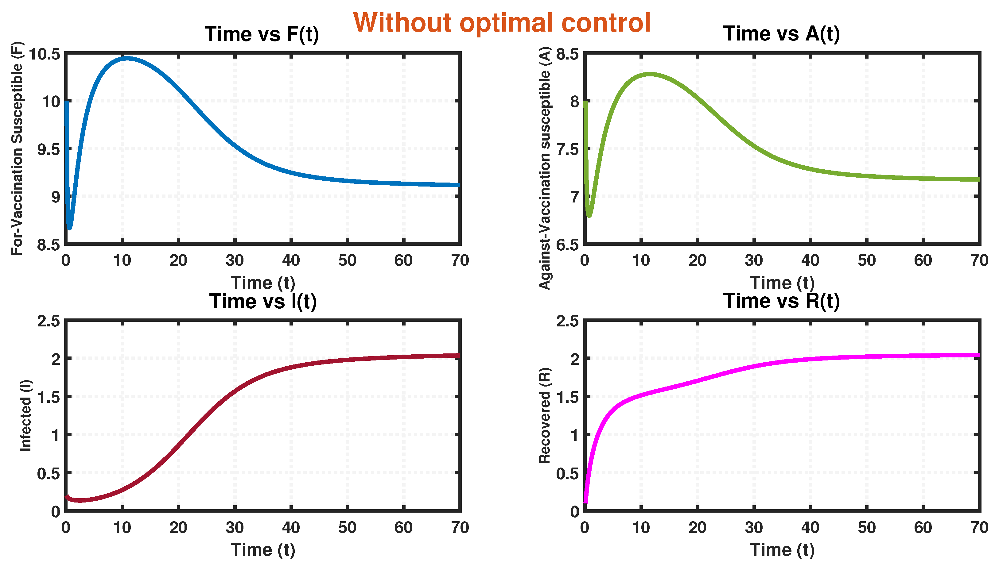
8. Numerical Simulation

In order to tackle the intricate nature of analytical problems, the application of numerical analysis becomes imperative. To facilitate this process, we employed MATLAB R2021a for conducting numerical simulations. These simulations allowed us to visually represent certain theoretical findings discussed earlier in this work. Specifically, we utilized MATLAB along with the Predictor-corrector PECE method, developed by Roberto Garrappa [46], to solve fractional differential equations. The parametric values used for these simulations can be found in the accompanying

Table 3. Value of parameters considered for numerical simulation.

Parameters	p	$\tilde{\mathsf{\Lambda }}\left(\mathsf{\Lambda }\right)$	$\tilde{\mathit{\beta }}\left(\mathit{\beta }\right)$	$\mathit{\alpha }$	b	k	$\tilde{\mathit{v}}\left(\mathit{v}\right)$	$\tilde{\mathit{\gamma }}\left(\mathit{\gamma }\right)$	$\tilde{\mathit{\eta }}\left(\mathit{\eta }\right)$	q	$\tilde{\mathit{\rho }}\left(\mathit{\rho }\right)$	$\tilde{\mathit{d}}\left(\mathit{d}\right)$	$\tilde{\mathit{\xi }}\left(\mathit{\xi }\right)$	$\tilde{\mathit{m}}\left(\mathit{m}\right)$
Values	$0.60$	$15\left(11.4415\right)$	$0.15\left(0.1813\right)$	$0.05$	$0.40$	2	$0.07\left(0.2030\right)$	$0.04\left(0.0552\right)$	$0.03\left(0.0426\right)$	$0.07$	$0.08\left(0.1030\right)$	$0.50\left(0.0675\right)$	$0.20\left(0.2349\right)$	$0.20\left(0.2349\right)$
Source	Estimated	[34]	Estimated	Estimated	[34]	[34]	Estimated	Estimated	Estimated	Estimated	Estimated	[34]	[34]	[34]

.

We have incorporated iterative schemes, namely Euler’s forward and backward methods, to address fractional-order optimal control problems. The procedure can be summarized as follows. The optimality system involves a two-point boundary value problem that encompasses a collection of fractional-order differential equations. The state system, denoted as (11), represents an initial value problem, while the adjoint system, referred to as (14), corresponds to a boundary value problem. To solve the state system, we have employed the forward iteration method, while the backward iteration method was employed to solve the costate system.

State system (11) is solved employing the iterative scheme below:

$$\begin{array}{cc}\hfill F\left(i\right)=& [p\mathsf{\Lambda }-\beta \left(1-\alpha \right){\left(1-b\right)}^{k}F(i-1)I(i-1)-vF(i-1)+\gamma A(i-1)-\eta F(i-1)+q\rho R(i-1)\hfill \\ \hfill & -dF(i-1)]h^{\nu }-\sum _{j=1}^{i}c\left(j\right)F(i-j)\hfill \\ \hfill A\left(i\right)=& [(1-p)\mathsf{\Lambda }-\beta \left(1-\alpha \right){\left(1-b\right)}^{k}A(i-1)I(i-1)-\gamma A(i-1)+\eta F\left(i\right)+(1-q)\rho R(i-1)\hfill \\ \hfill & -dA(i-1)]h^{\nu }-\sum _{j=1}^{i}c\left(j\right)A(i-j)\hfill \\ \hfill I\left(i\right)=& \left[\beta \left(1-\alpha \right){\left(1-b\right)}^k\left(F\left(i\right)+A\left(i\right)\right)I(i-1)-\xi I(i-1)-(d+m)I(i-1)\right]h^{\nu }\hfill \\ & -\sum _{j=1}^{i}c\left(j\right)I(i-j)\hfill \\ \hfill R\left(i\right)=& \left[vF\left(i\right)+\xi I\left(i\right)-(\rho +d)R(i-1)\right]h^{\nu }-\sum _{j=1}^{i}c\left(j\right)R(i-j)\hfill \end{array}$$

(15)

where, $c\left(0\right)=1$ and $c\left(j\right)=\left(1-{\displaystyle \frac{1+\nu }{j}}\right)c(j-1)$ and $h^{\nu }$ is the time step length. In each of the aforementioned systems of equations, the last term accounts for the memory component. Moving on to the adjoint system (14), a backward iteration method is implemented, imposing the terminal conditions ${\lambda }_i\left(T_f\right)=0(i=1,2,3,4)$. The optimal control is updated by the scheme below:

$${\alpha }_0=min\{max\left\{\alpha ,0\right\},1\},\mathrm{where}\alpha ={\displaystyle \frac{\beta {\left(1-b\right)}^k}{2w_2}}\left[({\lambda }_3\left(i\right)-{\lambda }_1\left(i\right))F\left(i\right)+({\lambda }_3\left(i\right)-{\lambda }_2\left(i\right))A\left(i\right)\right]I\left(i\right).$$

We have implemented an algorithm in MATLAB based on the aforementioned methodology. By fitting test data related to memory phenomena from various fields, we have observed that the fractional order can be interpreted as an index of memory. A higher value of the order parameter $\nu$ implies a slower rate of forgetting, and the dynamics of epidemic transmission heavily rely on the memory of previous stages [47]. The value of the order of fractional derivative ($\nu$) is required to be close to 1. Theoretically, we can explore fractional-order systems for values of $\nu$ ranging from 0 to 1. It is advisable to choose a value of $\nu$ close to 1 from the left. In certain cases, intriguing results are obtained when reducing the order of the derivative. However, for very small values of $\nu$, the MATLAB code becomes erroneous. Hence, it is essential to carefully select the order value. In our specific context, we have chosen the value of 0.9 (although it can be any value between 0.9 and 0.99) for conducting numerical simulations.

In this section, we have portrayed variation of $R_0$ with respect to $\beta ,\alpha ,b,k,\xi ,v,\gamma$ and $\eta$. Figure 4 and Figure 5, depict the analysis of sensitivity of various system parameters, along with their corresponding sensitivity indices. This analysis was conducted using the parameter values provided in Table 3. An increase in the transmission rate $\left(\beta \right)$ signifies higher chances of infection propagation within the system, resulting in the proliferation of disease. Conversely, an increase in each of governmental intervention $\left(\alpha \right)$, social interaction $\left(b\right)$, and public reaction $\left(k\right)$ yields a decrease in the basic reproduction number. This suggests that measures such as increased intervention by governing bodies, reduced social interactions, and favorable public responses contribute to mitigating the spread of disease, ultimately reducing the overall reproductive capacity of illness within the population. Furthermore, the prevalence of the illness can be partially controlled by two factors: improved medical care leading to a higher recovery rate among individuals and an increased vaccination rate. As more people recover from the sickness due to enhanced medical care and a greater number of individuals receive vaccinations, the overall impact of the illness can be mitigated. These parameters have inverse relationships with the basic reproduction number $R_0$. This indicates that by improving social behavior, enhancing public response, providing better treatment $\left(\xi \right)$ to infected individuals, and increasing the rate of vaccination $\left(v\right)$ among the individuals of the population, the epidemic situation can be controlled more effectively. In addition, it is shown how $R_0$ depends on the role of negative and positive attitudes towards vaccination. Also, it is seen that no transcritical bifurcation occurs with respect to $\gamma$ and $\eta$. The sensitivity indices for the parametric values of Table 3 are calculated as follows: ${\mathsf{{\rm Y}}}_{\beta }=1,{\mathsf{{\rm Y}}}_{\alpha }=-0.0723448,{\mathsf{{\rm Y}}}_b=-1.4566,{\mathsf{{\rm Y}}}_k=-1.0766,$ ${\mathsf{{\rm Y}}}_{\xi }=-0.233584,{\mathsf{{\rm Y}}}_v=-0.0201667,{\mathsf{{\rm Y}}}_{\gamma }=-0.0490857$ and ${\mathsf{{\rm Y}}}_{\eta }=0.00135574$, which are shown in Figure 5.

From earlier discussion, it is obtained that when $R_0<1$, DFE exists and is locally asymptotically stable. Again when $R_0>1$, there is an endemic equilibrium (EE) point that is stable. Based on our analysis, it is deduced that the equilibrium points undergo a stability exchange as they cross the critical threshold value $R_0=1$. According to [48], it can be said that the model (5) experiences a transcritical bifurcation at $R_0=1$. To provide a visual representation of these bifurcations, Figure 6 illustrates transcritical bifurcations associated with $\beta ,\alpha ,b,k$ and $\xi$ which describes that when the parameter level passes their corresponding threshold value, transcritical bifurcation occurs.

Figure 7a,b represent the variation in the time series of state variable $R\left(t\right)$ when $\gamma$ and $\eta$ vary and other parameters are fixed as in Table 3. It is seen that the number of recovered individuals increases with the raised level of $\gamma$. This indicates that quicker eradication of ailment is possible if more individuals are convinced to be vaccinated at an earlier stage of the pandemic crisis. On a similar note, when the value of $\eta$ grows, there is a corresponding decline in the number of recovered persons. In contrast, as shown in Figure 7c, DFE becomes stable when the vaccination rate $\left(v\right)$ crosses its corresponding bifurcation threshold value $v_t=0.468$. Moreover, a stable branch of endemic state is present only when the parameter lies below the critical point.

Next, using parametric values enlisted in Table 3, it is observed that $R_0=1.2197>1$ and so the condition for existence of endemic equilibrium is established. Hence, the system is locally asymptotically stable around $(9.0842,7.1496,2.0993,2.0675)$ as depicted in Figure 8. From this state, if we increase the value of b as $b=0.45$ and k as $k=2.5$, then Figure 9 provides an illustration of the convergence of trajectory of model (5) towards DFE with $R_0=0.7601<1$. The remaining model parameters can be found in Table 3, the figure portrays that trajectory starting from $(1,1.5,0.2,0.1)$ converge to $E_f(10.9748,8.7759,0,1.5669)$. This observation suggests that when the value of $R_0$ is greater than 1, the infection has effectively spread throughout the system, as evidenced by the convergence of the trajectory towards a non-zero equilibrium point. Figure 10a,b represent the variation of level of infected persons $I\left(t\right)$ when $\alpha$ and b vary for three different values of $\nu =0.9,0.95,1$. In Figure 10a, $\nu =0.9$ gives the transcritical bifurcation at ${\alpha }_t=0.2211$. If we take $\nu =0.95$, then transcritical bifurcation occurs at ${\alpha }_{t_1}=0.3204$. Lastly, for $\nu =1$ stability exchange exhibits at ${\alpha }_{t_2}=0.4066$ and endemic equilibrium disappears after exceeding the threshold ${\alpha }_{t_2}=0.4066$. These signify that if we consider fractional differential equations then the stability exchange achieves for lesser value of $\alpha$. A similar conclusion can be drawn for the model parameter b, which is depicted in Figure 10b.

In the proposed system (11), we have incorporated a control strategy called “governmental action” $\left(\alpha \right)$ to investigate its effectiveness in reducing the level of infection. The control interventions implemented in the model are assumed to be time-dependent. By utilizing a forward-backward iterative scheme, we have conducted numerical simulations to assess the impact of these control strategies on the overall behavior of the system. Through these simulations, we were able to observe and analyze the effects of control interventions on the dynamics and outcomes of the system [49]. Table 3 provides a comprehensive list of the parametric values, accompanied by the positive weight constants $w_1=10,$$w_2=15$. Furthermore, it is assumed that the control techniques under consideration will be consistently applied over a duration of two months, i.e., $T_f=70$ days.

Figure 11 provides a visualization of the dynamics of the model (11) when time-dependent control strategies are not considered. In this scenario, the population is $(9.1163,$$7.1741,2.0368,2.0422)$ at $T_f=70$. Let us now explore a scenario where governmental intervention varies over time. In Figure 12, we can observe the population profiles under the conditions of $\alpha ={\alpha }_0$. When $T_f=70$, the population is $(10.9470,8.7481,0,1.5586)$. It is noteworthy that as a result of the implementation of governmental measures aimed at minimizing disease transmission, an increasing number of individuals are becoming cautious of infection. Consequently, the size of susceptible individuals in the population is observed to rise in this particular situation. This observation highlights the impact of governmental interventions on influencing the dynamics of susceptible populations and the overall spread of infection.

The effectiveness of implemented control measures is often assessed based on their cost-effectiveness. In Figure 13, we can visualize the impact of time-dependent control measures $\alpha \left(t\right)$ on the cost design analysis $\left(J_0\right)$. In the absence of control measures, the cost incurred is primarily attributed to the impact of the diseased population on production loss. Without the implementation of effective control measures, there is a significant increase in the economic burden. Figure 14a provides an insightful depiction of the evolution of control intervention $\alpha$ over time. From this visualization, it is observed that $\alpha$ rises and achieves its highest value $\alpha =1$, at $t<15$, then remains constant. Figure 14b depicts the profile of infected individuals, represented by $I\left(t\right)$. As the level of governmental control strategies intensifies, we observe a corresponding decrease in the size of infected individuals over time. Figure 15 has illustrated how the simultaneous interaction of social behavior $\left(b\right)$, public reaction $\left(k\right)$, immunization rate $\left(v\right)$ and migration rates between for-vaccination and against-vaccination classes $(\gamma ,\eta )$ as well as the level of governmental control interventions have an influence on the level of infected and recovered compartments.

9. Conclusions

Epidemiological investigations possess remarkable qualities that enable a comprehensive understanding of the intricate dynamics within an epidemic system and identify various epidemiological factors that contribute to the complexity of the system. Over an extended period, researchers have dedicated significant efforts to study epidemic models of the SIRS type. However, more recently, the primary point of research in this field has shifted towards the exploration and evaluation of potential strategies for controlling and mitigating the impact of epidemics. The framework incorporates crucial factors such as governmental action, social behavior dynamics, and public response. Notably, the model accounts for two distinct susceptible states, characterized by individuals’ positive and negative attitudes towards vaccination. By considering these multifaceted elements, the study aims to provide a deeper understanding of disease transmission dynamics. Furthermore, we develop a fractional-order SIRS epidemic model that incorporates governmental interventions as a control mechanism.

Throughout the analysis of the model, we have observed the following insights:

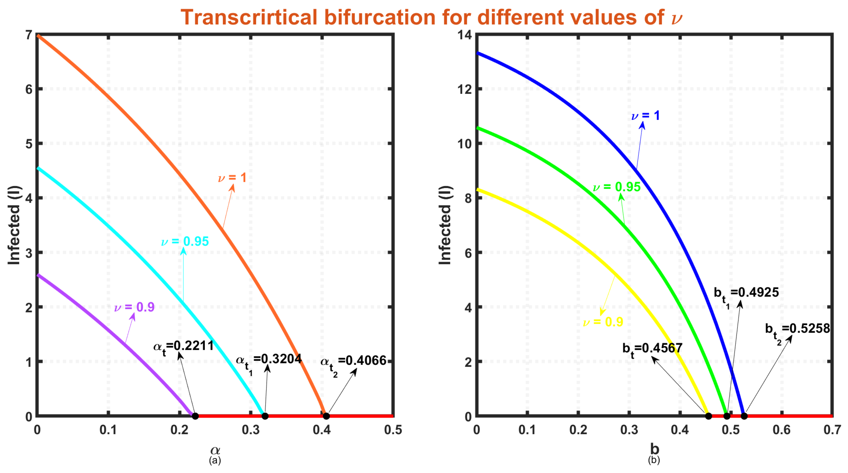
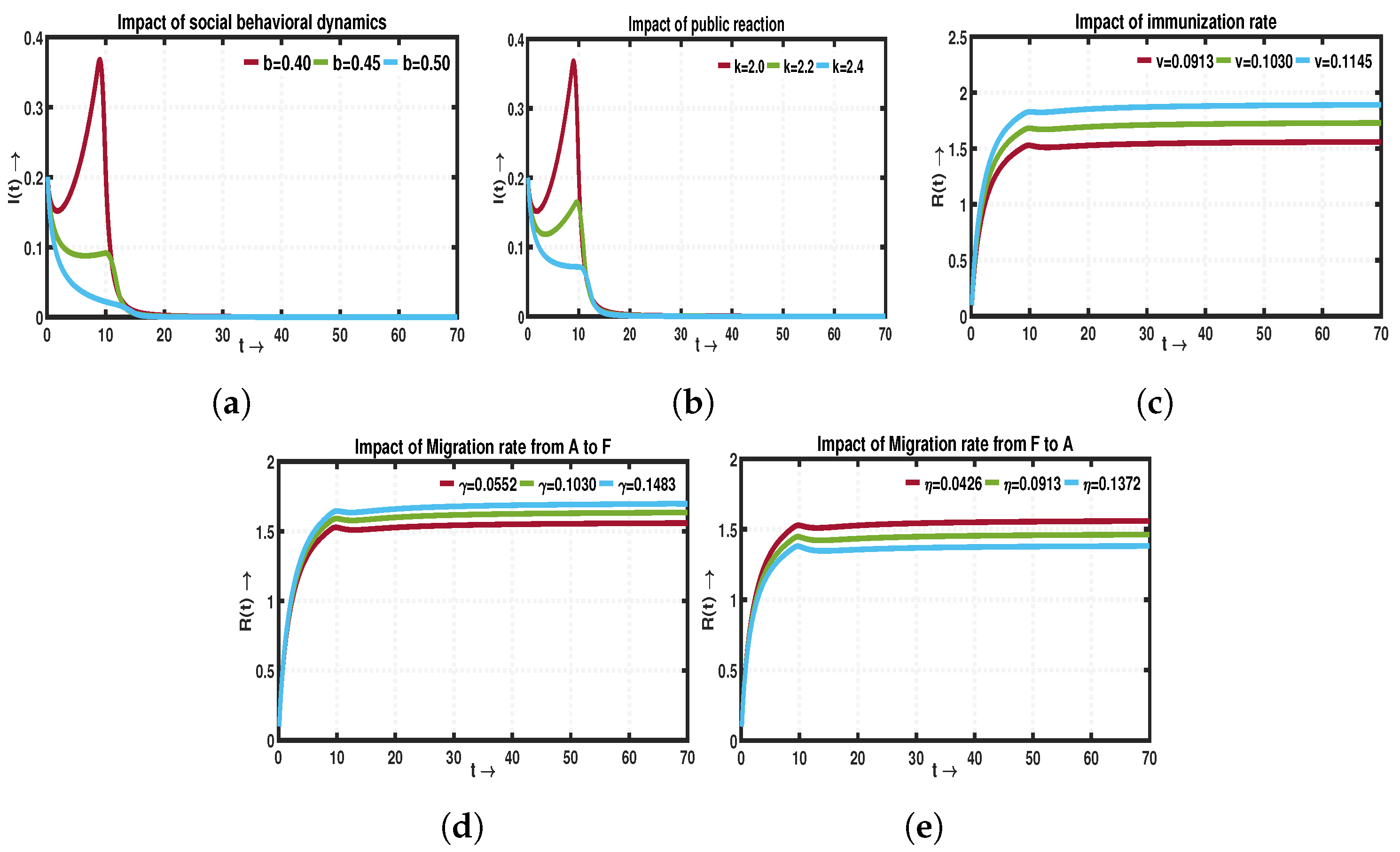
• Our findings demonstrate the better performance of the fractional-order model compared to the traditional integer-order model constructed using ordinary differential equations One limitation of integer-order systems is their inability to consider the historical information of the system, which is crucial in the context of disease transmission. When a disease spreads, the susceptible population relies on their past experiences and memory, to protect themselves from infection. In contrast, a dynamical system incorporating fractional-order derivatives encompasses not only the current state but also retains information about its previous states. Consequently, fractional-order systems provide a more comprehensive understanding of the underlying system dynamics compared to integer-order systems, as they take into account both present and past interactions and behaviors. In this study, a comprehensive investigation is conducted using a nonlinear SIRS compartmental framework to analyze the intricate dynamics of infectious diseases. The numerical section offers an in-depth analysis of various fractional and integer-order derivatives to gain insights into the complex dynamics of the proposed system. Figure 10a,b illustrate the variation in the level of infected individuals ($I\left(t\right)$) as $\alpha$ and b change for three different values of $\nu =0.9,0.95,1$. In Figure 10a, when $\nu =0.9$, a transcritical bifurcation occurs at ${\alpha }_t=0.2211$. For $\nu =0.95$, this bifurcation happens at ${\alpha }_{t_1}=0.3204$. When $\nu =1$, stability exchange is seen at ${\alpha }_{t_2}=0.4066$, and the endemic equilibrium disappears after surpassing ${\alpha }_{t_2}=0.4066$. These results indicate that using fractional differential equations results in stability exchange at a lower $\alpha$ value. A similar observation is made for the model parameter b, as shown in Figure 10b.
• Moreover, we have derived the explicit expression for the basic reproduction number, denoted as $R_0$. Additionally, our analysis reveals the existence of two feasible equilibriums within the system: the DFE and the EE. Notably, the disease-free state experiences a transcritical bifurcation when the basic reproduction number, represented by $R_0$, reaches unity ($R_0=1$). This critical point signifies a significant transition in the system’s behavior, where the disease-free state interacts with the endemic state, leading to fundamental changes in the dynamics of the system. Again, our observations indicate that both equilibria, namely DFE and EE, exhibit local asymptotic stability. This crucial property implies that the DFE serves as a threshold for the complete eradication of the disease, ensuring its elimination from the system. On the other hand, the local asymptotic stability of the EE signifies that the disease will persist within the system under specific parametric conditions. In the case of EE, complete eradication of the disease is not possible within the system.
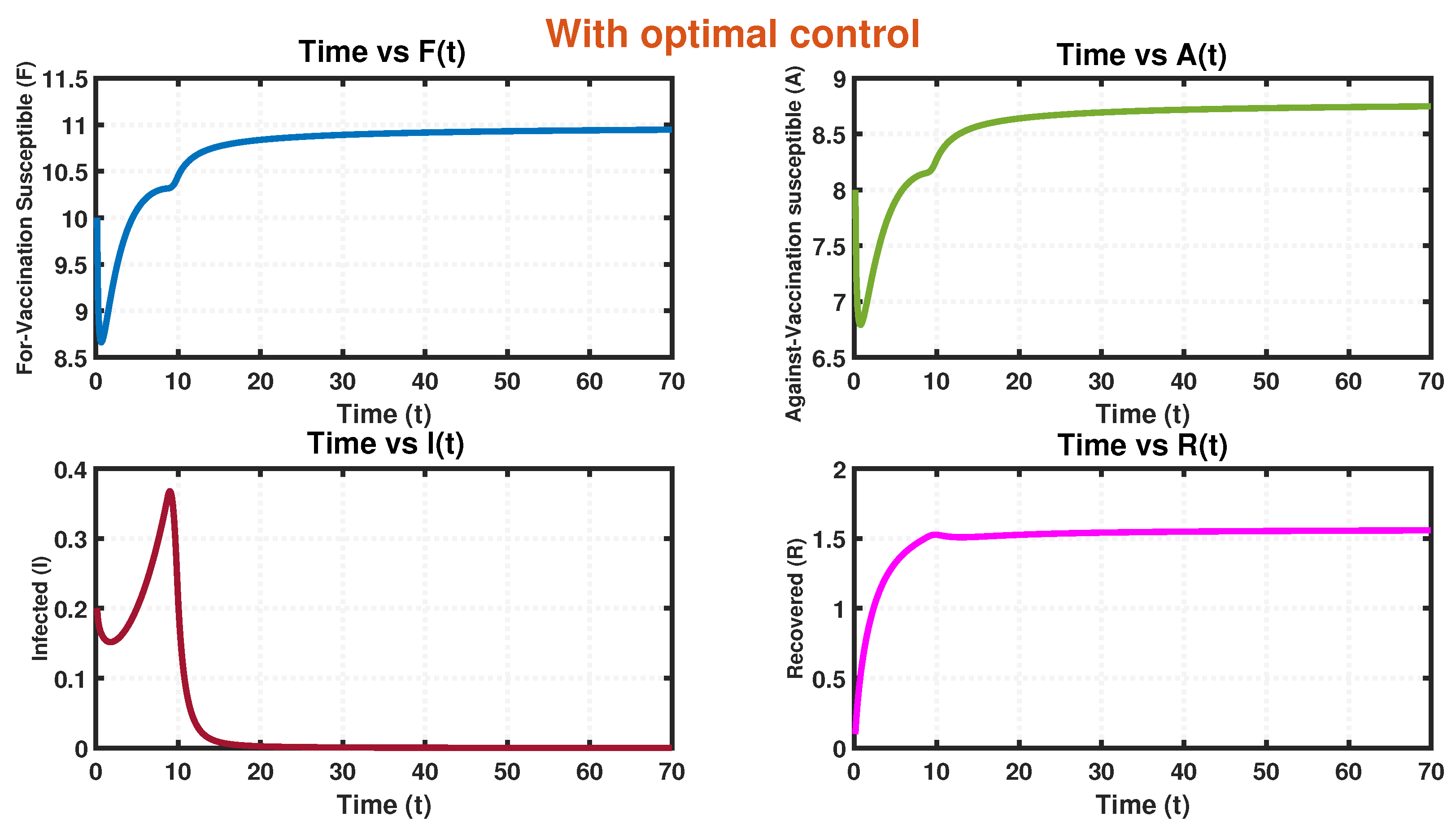
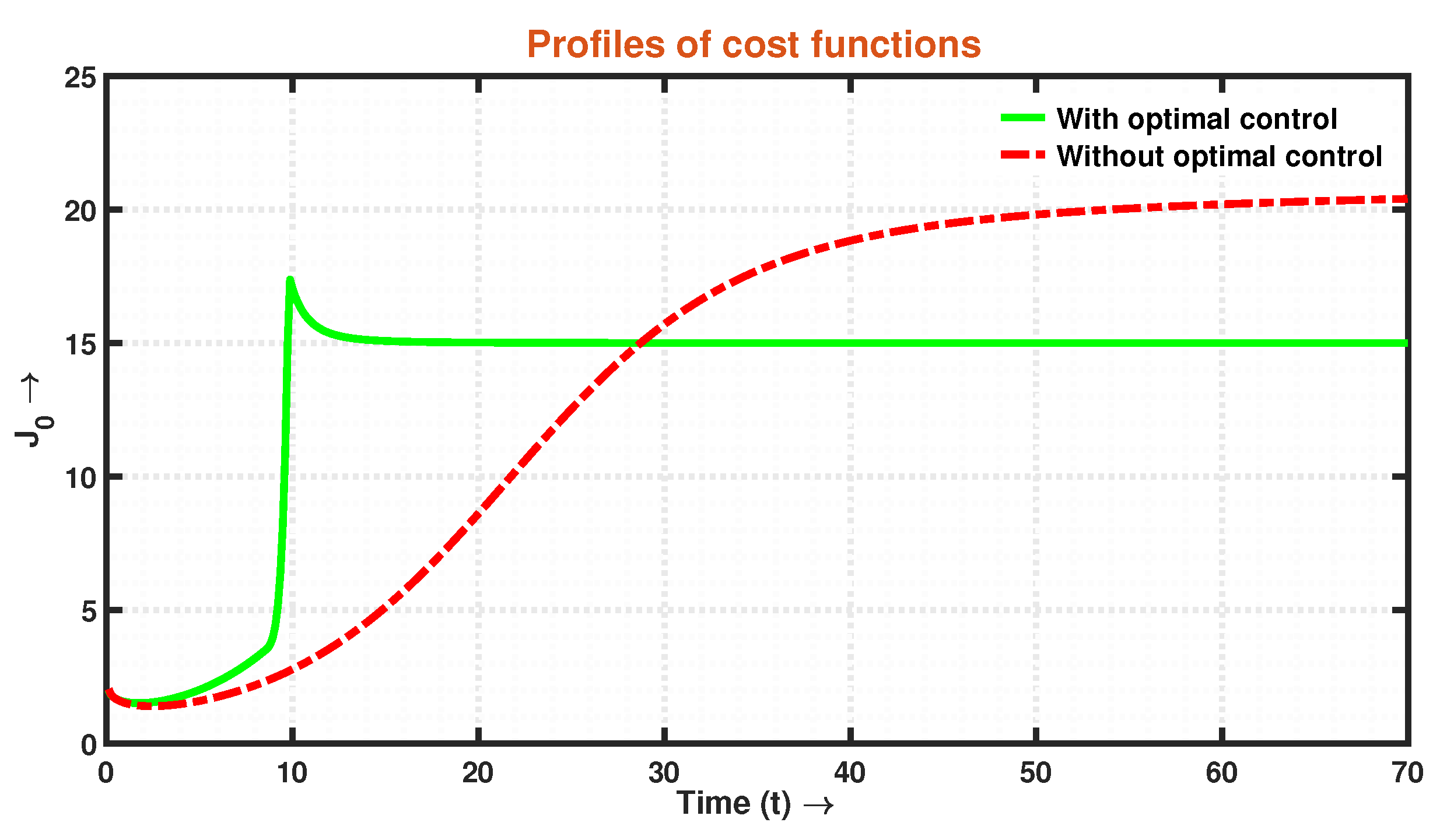
• Recognizing this challenge, we propose an associated optimal control problem to investigate the influence of governmental regulations on the dynamics of the system. The numerical simulations conducted in this study provide compelling evidence that the implementation of a control policy leads to a significant reduction in the size of infected individuals. This outcome implies that the adoption of control measures not only decreases the prevalence of the disease but also alleviates the economic burden associated with the epidemic. The findings highlight the effectiveness of the time-dependent control intervention in mitigating the spread of infection within a system during an epidemic outbreak. This control strategy proves to be instrumental in curbing infectivity, ultimately yielding positive outcomes in disease management and the overall well-being of the affected population.

10. Future Research Scope

In future research, there is potential for further extending our model by incorporating additional compartments such as a quarantine compartment or an exposed compartment. Moreover, considering media awareness as a control measure could be explored to enhance the effectiveness of disease management strategies. Additionally, the deterministic system can be modified to a stochastic system, accounting for the influence of white noise, in order to examine the dynamic behavior of the stochastic model. It is worth noting that the pandemic situation is influenced by numerous factors, including economic and financial aspects. Therefore, in our future endeavors, we aim to incorporate and investigate these important factors to gain a more comprehensive understanding of their role in controlling and managing the spread of infectious diseases.

References

1. Podlubny, I. An introduction to fractional derivatives, fractional differential equations, to methods of their solution and some of their applications. Math. Sci. Eng 1999, 198, 340. [Google Scholar]
2. Petráš, I. Fractional-Order Nonlinear Systems: Modeling, Analysis and Simulation; Springer Science & Business Media: Berlin/Heidelberg, Germany, 2011. [Google Scholar]
3. Teodoro, G.S.; Machado, J.T.; De Oliveira, E.C. A review of definitions of fractional derivatives and other operators. J. Comput. Phys. 2019, 388, 195–208. [Google Scholar] [CrossRef]
4. Kai, Y.; Chen, S.; Zhang, K.; Yin, Z. Exact solutions and dynamic properties of a nonlinear fourth-order time-fractional partial differential equation. Waves Random Complex Media 2022, 2044541. [Google Scholar] [CrossRef]
5. Li, M.; Wang, L.; Luo, C.; Wu, H. A new improved fractional Tikhonov regularization method for moving force identification. Structures 2024, 60, 105840. [Google Scholar] [CrossRef]
6. Kumar, P.; Erturk, V.S.; Abboubakar, H.; Nisar, K.S. Prediction studies of the epidemic peak of coronavirus disease in Brazil via new generalised Caputo type fractional derivatives. Alex. Eng. J. 2021, 60, 3189–3204. [Google Scholar] [CrossRef]
7. Zafar, Z.U.A.; Ali, N.; Baleanu, D. Dynamics and numerical investigations of a fractional-order model of toxoplasmosis in the population of human and cats. Chaos Solitons Fractals 2021, 151, 111261. [Google Scholar] [CrossRef]
8. Zafar, Z.U.A.; Zaib, S.; Hussain, M.T.; Tunç, C.; Javeed, S. Analysis and numerical simulation of tuberculosis model using different fractional derivatives. Chaos Solitons Fractals 2022, 160, 112202. [Google Scholar] [CrossRef]
9. Nisar, K.S.; Farman, M.; Abdel-Aty, M.; Cao, J. A review on epidemic models in sight of fractional calculus. Alex. Eng. J. 2023, 75, 81–113. [Google Scholar] [CrossRef]
10. Azeem, M.; Farman, M.; Abukhaled, M.; Nisar, K.S.; AKGÜL, A. Epidemiological Analysis Of Human Liver Model with Fractional Operator. Fractals 2023, 31, 2340047. [Google Scholar] [CrossRef]
11. Nisar, K.S.; Farman, M.; Abdel-Aty, M.; Abdel-Aty, M. Mathematical Epidemiology: A Review of the Singular and Non-Singular Kernels and their Applications. Prog. Fract. Differ. Appl. 2023, 9, 507–544. [Google Scholar] [CrossRef]
12. Zafar, Z.U.A.; DarAssi, M.H.; Ahmad, I.; Assiri, T.A.; Meetei, M.Z.; Khan, M.A.; Hassan, A.M. Numerical simulation and analysis of the stochastic hiv/aids model in fractional order. Results Phys. 2023, 53, 106995. [Google Scholar] [CrossRef]
13. Vitanov, N.K.; Ausloos, M.R. Knowledge epidemics and population dynamics models for describing idea diffusion. In Models of Science Dynamics: Encounters between Complexity Theory and Information Sciences; Springer: Berlin/Heidelberg, Germany, 2011; pp. 69–125. [Google Scholar] [CrossRef]
14. Larson, H.J.; Jarrett, C.; Eckersberger, E.; Smith, D.M.; Paterson, P. Understanding vaccine hesitancy around vaccines and vaccination from a global perspective: A systematic review of published literature, 2007–2012. Vaccine 2014, 32, 2150–2159. [Google Scholar] [CrossRef]
15. Lin, C.; Tu, P.; Beitsch, L.M. Confidence and receptivity for COVID-19 vaccines: A rapid systematic review. Vaccines 2020, 9, 16. [Google Scholar] [CrossRef]
16. Piedrahita-Valdés, H.; Piedrahita-Castillo, D.; Bermejo-Higuera, J.; Guillem-Saiz, P.; Bermejo-Higuera, J.R.; Guillem-Saiz, J.; Sicilia-Montalvo, J.A.; Machío-Regidor, F. Vaccine hesitancy on social media: Sentiment analysis from June 2011 to April 2019. Vaccines 2021, 9, 28. [Google Scholar] [CrossRef]
17. Reiter, P.L.; Pennell, M.L.; Katz, M.L. Acceptability of a COVID-19 vaccine among adults in the United States: How many people would get vaccinated? Vaccine 2020, 38, 6500–6507. [Google Scholar] [CrossRef]
18. Bonte, J. The Continuum of Attitudes towards Vaccination A Qualitative Analysis of Arguments Used in Pro-, Anti-and Hesitant Tweets. Master’s Thesis, Utrecht University, Utrecht, The Netherlands, 2022. [Google Scholar]
19. Lee, S.K.; Sun, J.; Jang, S.; Connelly, S. Misinformation of COVID-19 vaccines and vaccine hesitancy. Sci. Rep. 2022, 12, 13681. [Google Scholar] [CrossRef]
20. Wang, Q.; Jiang, Q.; Yang, Y.; Pan, J. The burden of travel for care and its influencing factors in China: An inpatient-based study of travel time. J. Transp. Health 2022, 25, 101353. [Google Scholar] [CrossRef]
21. Nisar, K.S.; Shoaib, M.; Raja, M.A.Z.; Tabassum, R.; Morsy, A. A novel design of evolutionally computing to study the quarantine effects on transmission model of Ebola virus disease. Results Phys. 2023, 48, 106408. [Google Scholar] [CrossRef]
22. Dutta, P.; Saha, S.; Samanta, G. Assessing the influence of public behavior and governmental action on disease dynamics: A PRCC analysis and optimal control approach. Eur. Phys. J. Plus 2024, 139, 527. [Google Scholar] [CrossRef]
23. Agrawal, O.P. A general formulation and solution scheme for fractional optimal control problems. Nonlinear Dyn. 2004, 38, 323–337. [Google Scholar] [CrossRef]
24. Kheiri, H.; Jafari, M. Optimal control of a fractional-order model for the HIV/AIDS epidemic. Int. J. Biomath. 2018, 11, 1850086. [Google Scholar] [CrossRef]
25. Al-Basir, F.; Elaiw, A.M.; Kesh, D.; Roy, P.K. Optimal control of a fractional-order enzyme kinetic model. Control. Cybern. 2015, 44, 443–461. [Google Scholar]
26. Akman Yıldız, T. Optimal control problem of a non-integer order waterborne pathogen model in case of environmental stressors. Front. Phys. 2019, 7, 95. [Google Scholar] [CrossRef]
27. Kada, D.; Kouidere, A.; Balatif, O.; Rachik, M.; Labriji, E.H. Mathematical modeling of the spread of COVID-19 among different age groups in Morocco: Optimal control approach for intervention strategies. Chaos Solitons Fractals 2020, 141, 110437. [Google Scholar] [CrossRef] [PubMed]
28. Khajji, B.; Kada, D.; Balatif, O.; Rachik, M. A multi-region discrete time mathematical modeling of the dynamics of Covid-19 virus propagation using optimal control. J. Appl. Math. Comput. 2020, 64, 255–281. [Google Scholar] [CrossRef] [PubMed]
29. Kumar, P.; Govindaraj, V.; Erturk, V.S.; Nisar, K.S.; Inc, M. Fractional mathematical modeling of the Stuxnet virus along with an optimal control problem. Ain Shams Eng. J. 2023, 14, 102004. [Google Scholar] [CrossRef]
30. Hussain, T.; Ozair, M.; Faizan, M.; Jameel, S.; Nisar, K.S. Optimal control approach based on sensitivity analysis to retrench the pine wilt disease. Eur. Phys. J. Plus 2021, 136, 1–27. [Google Scholar] [CrossRef]
31. Li, H.L.; Zhang, L.; Hu, C.; Jiang, Y.L.; Teng, Z. Dynamical analysis of a fractional-order predator-prey model incorporating a prey refuge. J. Appl. Math. Comput. 2017, 54, 435–449. [Google Scholar] [CrossRef]
32. Ahmed, E.; Elgazzar, A. On fractional order differential equations model for nonlocal epidemics. Phys. A Stat. Mech. Its Appl. 2007, 379, 607–614. [Google Scholar] [CrossRef] [PubMed]
33. Das, M.; Samanta, G.; De la Sen, M. A Fractional Order Model to Study the Effectiveness of Government Measures and Public Behaviours in COVID-19 Pandemic. Mathematics 2022, 10, 3020. [Google Scholar] [CrossRef]
34. Saha, S.; Dutta, P.; Samanta, G. Dynamical behavior of SIRS model incorporating government action and public response in presence of deterministic and fluctuating environments. Chaos Solitons Fractals 2022, 164, 112643. [Google Scholar] [CrossRef]
35. Dutta, S.; Dutta, P.; Samanta, G. Modelling disease transmission through asymptomatic carriers: A societal and environmental perspective. Int. J. Dyn. Control. 2024. [Google Scholar] [CrossRef]
36. Li, Y.; Chen, Y.; Podlubny, I. Stability of fractional-order nonlinear dynamic systems: Lyapunov direct method and generalized Mittag–Leffler stability. Comput. Math. Appl. 2010, 59, 1810–1821. [Google Scholar] [CrossRef]
37. Ghosh, U.; Pal, S.; Banerjee, M. Memory effect on Bazykin’s prey-predator model: Stability and bifurcation analysis. Chaos Solitons Fractals 2021, 143, 110531. [Google Scholar] [CrossRef]
38. Van den Driessche, P.; Watmough, J. Reproduction numbers and sub-threshold endemic equilibria for compartmental models of disease transmission. Math. Biosci. 2002, 180, 29–48. [Google Scholar] [CrossRef] [PubMed]
39. Matouk, A. Stability conditions, hyperchaos and control in a novel fractional order hyperchaotic system. Phys. Lett. A 2009, 373, 2166–2173. [Google Scholar] [CrossRef]
40. Guo, T.L. The necessary conditions of fractional optimal control in the sense of Caputo. J. Optim. Theory Appl. 2013, 156, 115–126. [Google Scholar] [CrossRef]
41. Ndaïrou, F.; Torres, D.F. Distributed-Order Non-Local Optimal Control. Axioms 2020, 9, 124. [Google Scholar] [CrossRef]
42. Das, M.; Samanta, G.P. Optimal control of a fractional order epidemic model with carriers. Int. J. Dyn. Control. 2022, 10, 598–619. [Google Scholar] [CrossRef]
43. Das, M.; Samanta, G.; De la Sen, M. Stability analysis and optimal control of a fractional order synthetic drugs transmission model. Mathematics 2021, 9, 703. [Google Scholar] [CrossRef]
44. Gaff, H.; Schaefer, E. Optimal control applied to vaccination and treatment strategies for various epidemiological models. Math. Biosci. Eng. 2009, 6, 469–492. [Google Scholar] [CrossRef] [PubMed]
45. Kassa, S.M.; Ouhinou, A. The impact of self-protective measures in the optimal interventions for controlling infectious diseases of human population. J. Math. Biol. 2015, 70, 213–236. [Google Scholar] [CrossRef] [PubMed]
46. Garrappa, R. On linear stability of predictor–corrector algorithms for fractional differential equations. Int. J. Comput. Math. 2010, 87, 2281–2290. [Google Scholar] [CrossRef]
47. Du, M.; Wang, Z.; Hu, H. Measuring memory with the order of fractional derivative. Sci. Rep. 2013, 3, 3431. [Google Scholar] [CrossRef]
48. Guckenheimer, J.; Holmes, P. Nonlinear Oscillations, Dynamical Systems, and Bifurcations of Vector Fields; Springer Science & Business Media: Berlin/Heidelberg, Germany, 2013; Volume 42. [Google Scholar]
49. Cao, X.; Datta, A.; Al Basir, F.; Roy, P.K. Fractional-order model of the disease psoriasis: A control based mathematical approach. J. Syst. Sci. Complex. 2016, 29, 1565–1584. [Google Scholar] [CrossRef]
Figure 1. Schematic representation of system (5).
Mathematics 12 02232 g001
Figure 2. Stability region of fractional-order system.
Mathematics 12 02232 g002
Figure 3. Changes of population dynamics with respect to reproduction number ( R 0 ). Here, (a) represents R 0 Vs F ( t ) graph showing that the sizes of for-vaccination susceptible are decreasing as R 0 crosses 1, (b) represents R 0 Vs A ( t ) graph showing that the size of against-vaccination susceptible decreases as R 0 crosses 1, (c) represents R 0 Vs I ( t ) graph showing that the size of infected population increases as R 0 crosses 1 and (d) represents R 0 Vs R ( t ) graph showing that the size of recovered population increases as R 0 crosses 1.
Mathematics 12 02232 g003
Figure 4. Profile of basic reproduction number with the changes of β , α , b , k , ξ , v , γ and η in system (5). Here, (a,h) represent that R 0 increases as β , η increase. (bg) represent that R 0 decreases as α , b , k , ξ , v , γ increase. Here, the black dashed lines presents the level of R 0 = 1 .
Mathematics 12 02232 g004
Figure 5. Sensitivity index of β , α , b , k , ξ , v , γ and η of system (5).
Mathematics 12 02232 g005
Figure 6. Occurrence of transcritical bifurcation for model (5) considering β , α , b , k and ξ as bifurcation parameter. (a,b) represent the bifurcation diagrams with respect to β , from the figures we see that at β t = 0.1483 transcritical bifurcation occurs between disease-free equilibrium ( E f ) and endemic equilibrium point ( E ). The bifurcation diagrams of α , b and k with respect to I ( t ) in (ce) show that the transcritical bifurcations occur at α t = 0.2570 , b t = 0.4567 and k t = 2.3887 , respectively. (f) is the bifurcation diagram of ξ with respect to R ( t ) , here transcritical bifurcation occurs at ξ t = 0.4581 . In all the sub-figures solid curve indicates stable branch and dashed curve implies unstable branch of the steady states.
Mathematics 12 02232 g006
Figure 7. Impact of γ , η and v on system (5). Here, (a) represents that level of recovered class increases when γ increases. Here, (b) represents that level of recovered class decreases when η increases. (c) represents the bifurcation diagram with respect to v, from the figure we see that at v t = 0.468 transcritical bifurcation occurs between disease-free equilibrium ( E f ) and endemic equilibrium point ( E ).
Mathematics 12 02232 g007
Figure 8. Time series of system (5) corresponds to Table 3 when E = ( 9.0842 , 7.1496 , 2.0993 , 2.0675 ) and R 0 = 1.2197 > 1 .
Mathematics 12 02232 g008
Figure 9. Time series of system (5) corresponds to Table 3 when E f = ( 10.9748 , 8.7759 , 0 , 1.5669 ) and R 0 = 0.7601 < 1 .
Mathematics 12 02232 g009
Figure 10. Variation of state variable I ( t ) when α and b vary for different values of ν = 0.9 , 0.95 , 1 . (a) shows that when ν = 0.9 , the transcritical bifurcation occurs at α t = 0.2211 , when ν = 0.95 , the transcritical bifurcation occurs at α t = 0.3204 and when ν = 1 , the transcritical bifurcation occurs at α t = 0.4066 . (b) shows that when ν = 0.9 , the transcritical bifurcation occurs at b t = 0.4567 , when ν = 0.95 , the transcritical bifurcation occurs at b t = 0.4925 and when ν = 1 , the transcritical bifurcation occurs at b t = 0.5258 . By considering fractional differential equations, the stability exchange achieves for lesser values of α and b.
Mathematics 12 02232 g010
Figure 11. Diagrams of the population in absence of optimal control.
Mathematics 12 02232 g011
Figure 12. Diagrams of the population in presence of optimal control α 0 .
Mathematics 12 02232 g012
Figure 13. Cost profiles of J 0 for time-dependent control strategies and without control strategies.
Mathematics 12 02232 g013
Figure 14. (a) Profile of optimal control α 0 , (b) Change of infection level for time-dependent control strategies.
Mathematics 12 02232 g014
Figure 15. Influence of b , k , v , γ , η as well as the level of control interventions to the amount of infected and recovered compartments. Here, (a,b) represent amount of infected people decreases as b and k are increased. Again (c,d) represent amount of recovered people increases as v and γ are increased. And (e) shows that recovered people decreases as η increases.
Mathematics 12 02232 g015