
Predicting Pump Inspection Cycles for Oil Wells Based on Stacking Ensemble Models


Abstract
1. Introduction
1.1. Literature Review
1.2. Motivation and Organization
2. Machine Learning Methods
3. The Two-Layer Improved Stacking Ensemble Model
3.1. The Ensemble Model
3.2. The Stacking Model
4. Design of the Experiment
4.1. Data Set Establishment and Data Preprocessing
- Production days: The days that a pumpjack work properly, denoted by d.
- Water cut: The percentage (%) of water in the oil produced from the pumping well.
- Pump depth: The depth in meters (m) from the wellhead to the pump.
- Permeability: The ability in millidarcy (mD) of a rock to allow fluid to pass through under a certain pressure difference.
- Maximum load: The pumping unit has a maximum load in kilonewton (kN) at the overhang on the upstroke.
- Minimum load: The minimum load in kilonewton (kN) on the suspension point of the pumping unit during the downstroke.
- Maximum well deviation angle: The maximum angle in degree (°) between the tangent at the measurement point on the axis of the oil well and the vertical line.
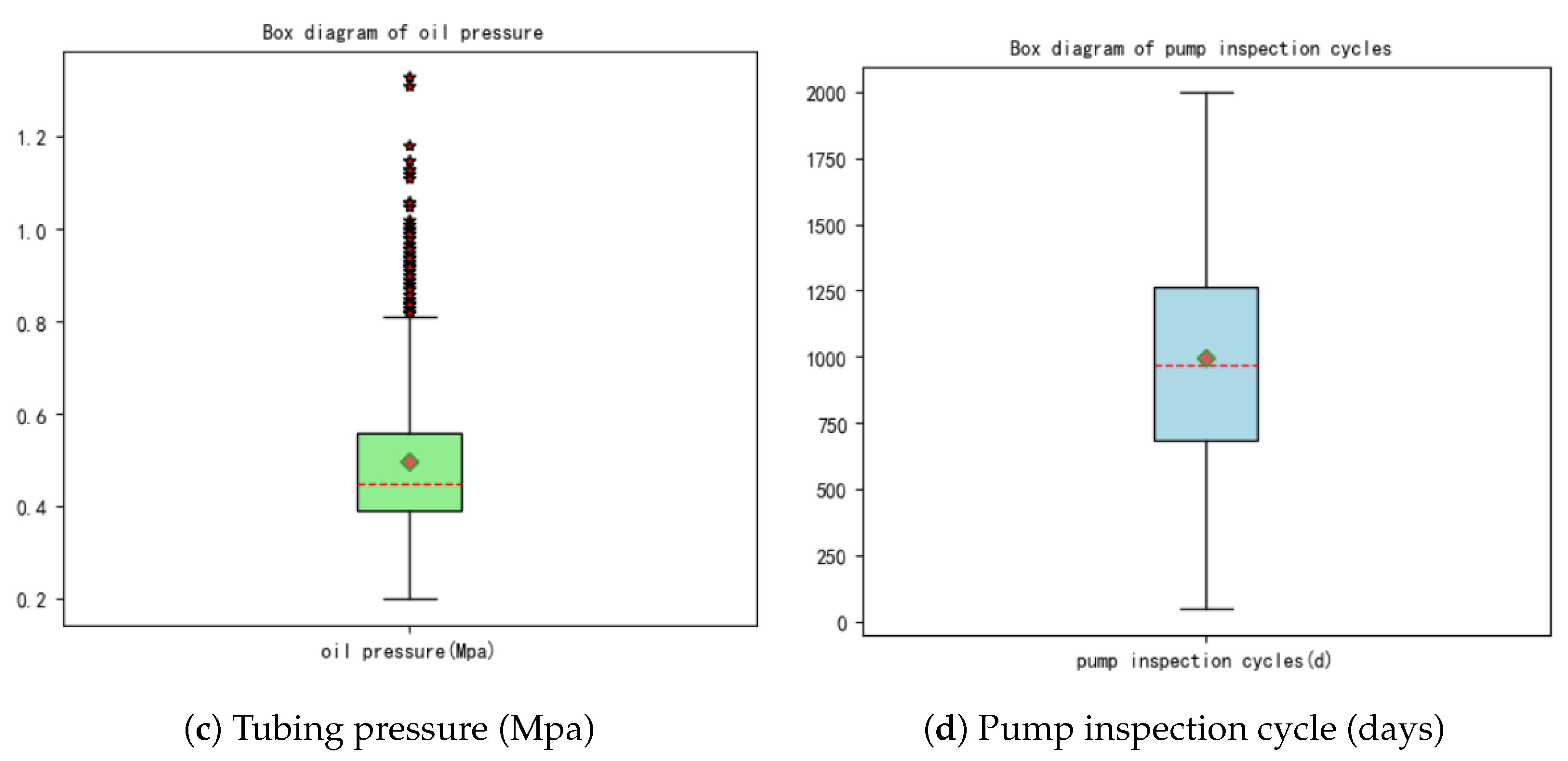
- Oil pressure: The residual pressure megapascal (MPa) of the oil flow from the bottom of the well to the wellhead.
- Casing pressure: The residual pressure in MPa that lifts the oil and gas from the we; bottom through the annular space between the tubing and casing to the wellhead.
- Stroke: The distance in m the piston travels in one up-and-down motion.
- Stroke count: The number of times the pumping rod reciprocates up and down per minute, denoted by .
- Daily oil production: Mean oil production in tons (t).
- Oil concentration: The polymer concentration in the produced oil (%).
- Oil viscosity: The polymer viscosity in milligrams per liter () in the produced oil.
- Static pressure: The pressure in MPa exerted on an object surface due to the fluid’s weight and the intermolecular forces among the fluid molecules, when the fluid is at rest or in uniform linear motion.
- Sucker rod length: The total cumulative length in m of all the sucker rods in the oil well.
- Flow pressure: The pressure in MPa measured in the middle of the oil and gas when the well is normally producing.
- Tubing length: The total cumulative length in m of all the tubes in the oil well.
4.2. Feature Selection and Grid Search Method
4.3. Model Establishment
- The metalearner’s learning space is limited because of data repetition during learning. Complex models could lead to overfitting, while simple models often yield better results, especially those with anti-overfitting characteristics.
- The training performance of the metalearners with a complex model is often unreliable, making it challenging to optimize them. Therefore, in most cases, we opt for simple models for modeling.
- Effective metalearners (optimized through hyperparameter tuning) combined with bagging can sometimes enhance the metalearner’s learning capacity.
Model Evaluation
5. Results and Findings
5.1. Data Preprocessing Results
5.2. Feature Selection Results
5.3. Model Prediction Results
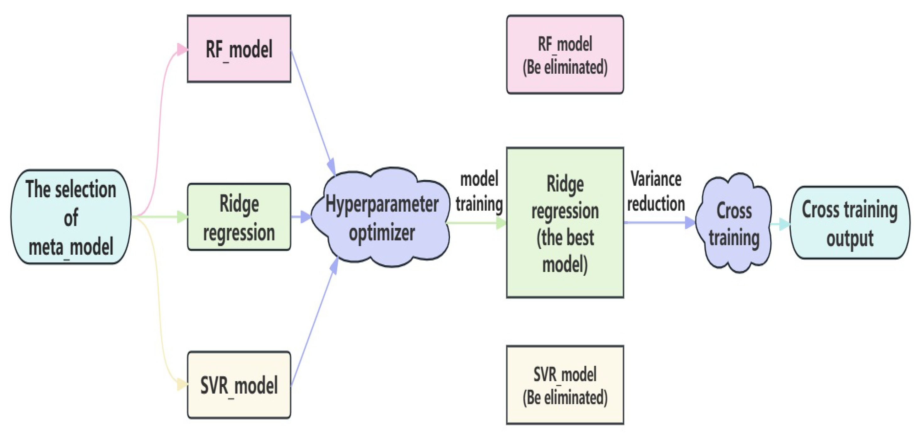
- We use ridge regression, RF, and SVR as regression models for metalearner training.
- A hyperparameter optimizer tunes the metalearner’s hyperparameters to obtain the best model.
- We evaluate the final learning performance of the three models, as shown in Table 4.
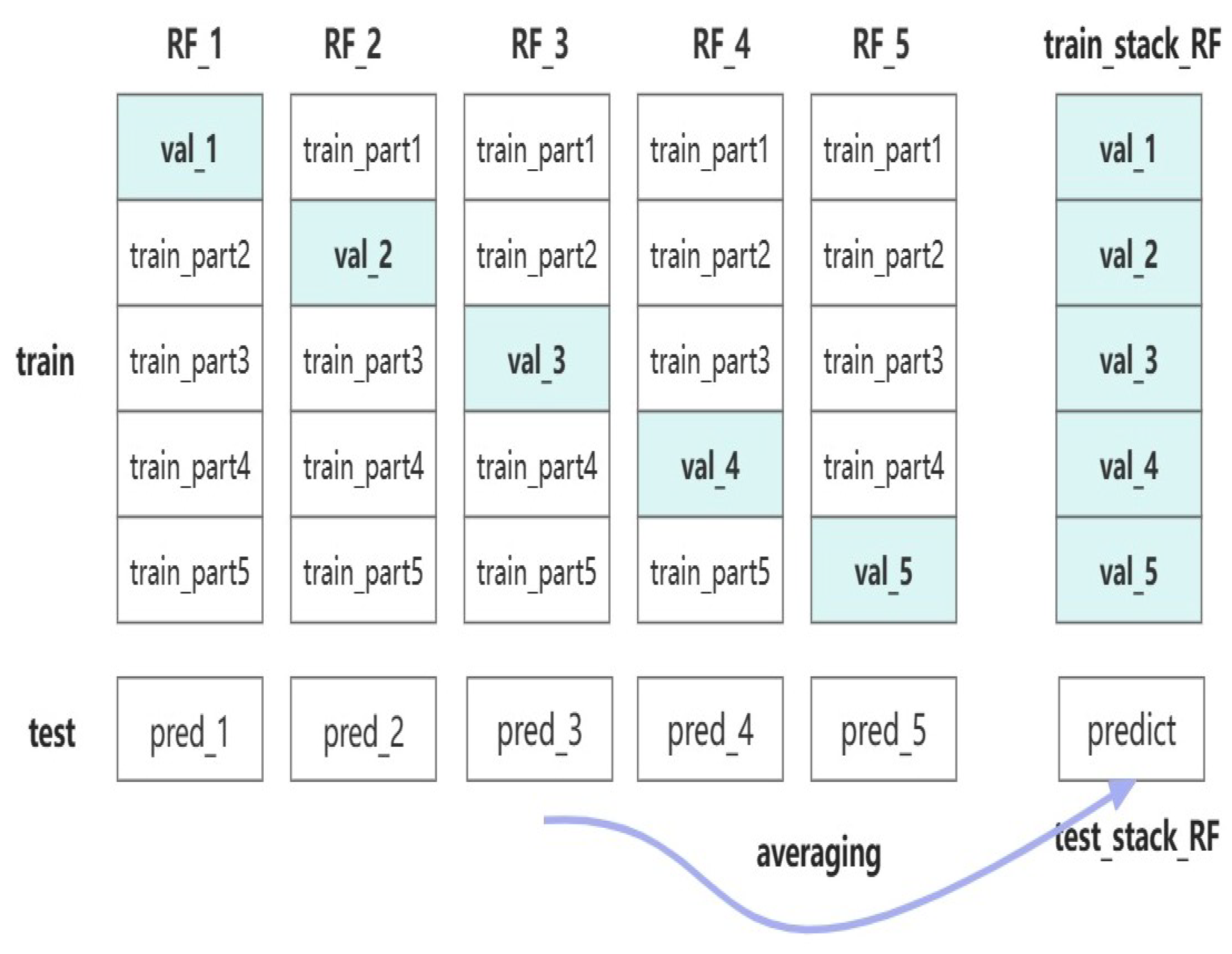
- The cleaned data are split into training, validation, and test sets. The proportions of the training and test sets are the same as for individual models. We further divide the training set into a 20% validation subset and an 80% training subset. The base models are trained on the training subset, and the trained base models are then used on the validation subset. The validation set predictions serve as input features for the metalearner tested on the test set.
- The base models are trained and fitted on the training subset. Their predictions on the validation and test sets are stacked to create input features for the metalearner.
- The metalearner of ridge regression is trained on the new features and labels generated from the validation set. The trained ridge regression model predicts the new features, resulting in the final well-trained pump inspection cycle prediction model. Figure 7 illustrates the stacking ensemble model flow of the proposed two-layer stacking ensemble model.
5.4. Technical Application
5.5. Discussion
- Diversity among weak classifiers: The stacking ensemble model combines classifiers with different decision boundaries, resulting in more reasonable boundaries and reduced overall errors.
- Greater flexibility: Ensemble learning provides flexibility.
- Improved fit on training data: The stacking ensemble model can outperform individual models on training data while mitigating overfitting risks.
6. Conclusions
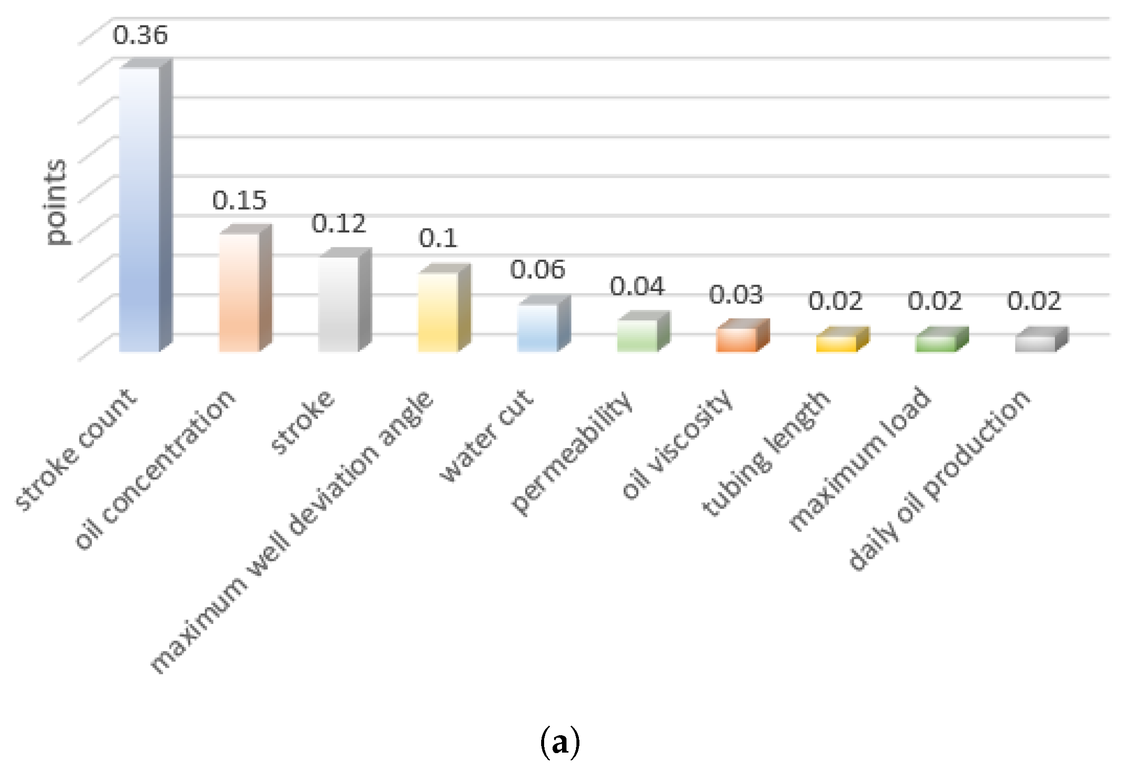
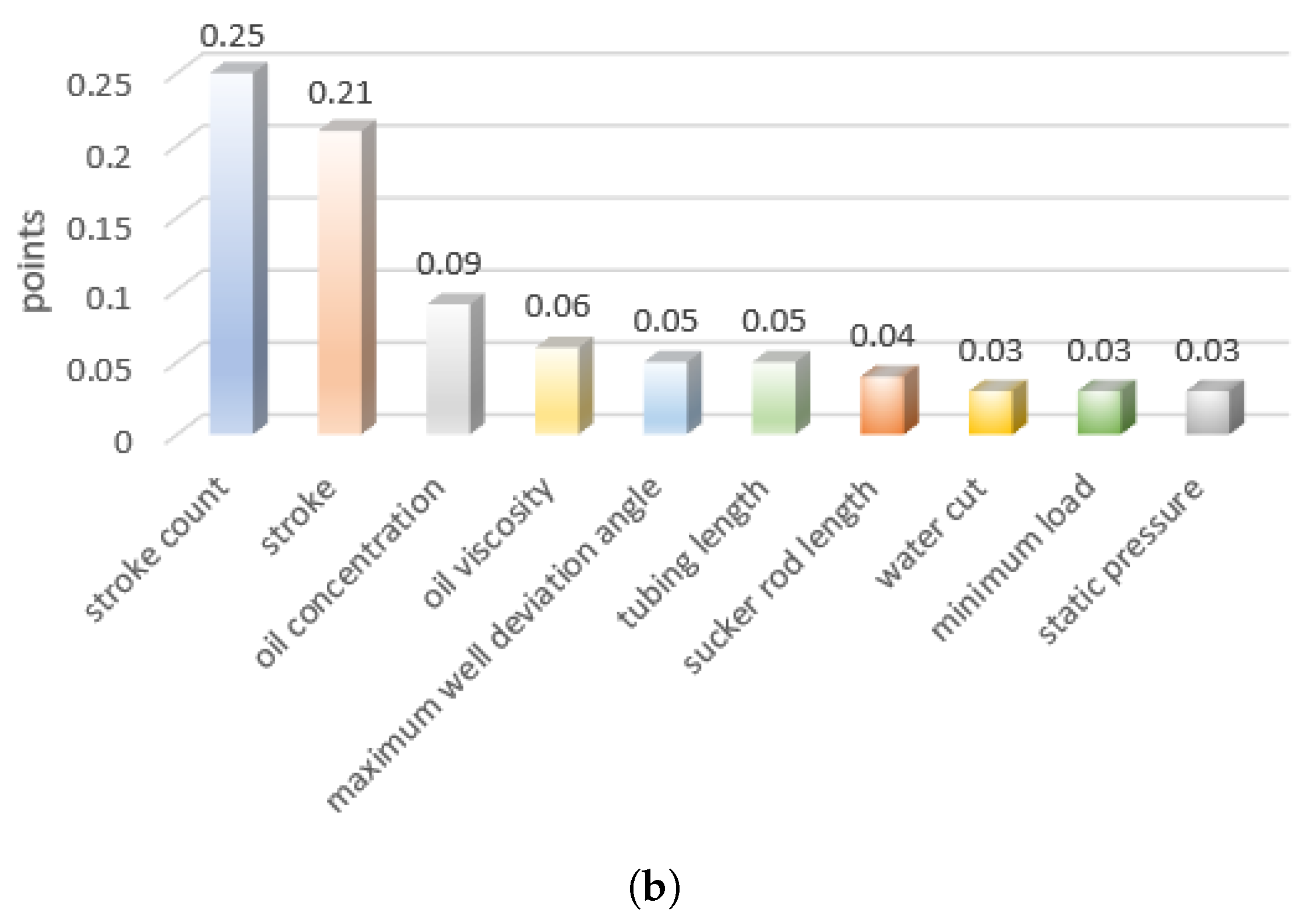
- Combining theoretical analysis, field guidance, and data mining, we analyze the factors affecting pump inspection cycles. We use a comprehensive evaluation model that combines feature selection using RF and XGBoost to identify the ten most significant factors influencing pump inspection cycles.
- We select RF, LightGBM, SVR, and AdaBoost regression models to predict pump inspection cycles. The results show that RF achieved the highest accuracy of 90.19%, followed by LightGBM with 88.77%, SVR with 86.16%, and AdaBoost with 83.24%.
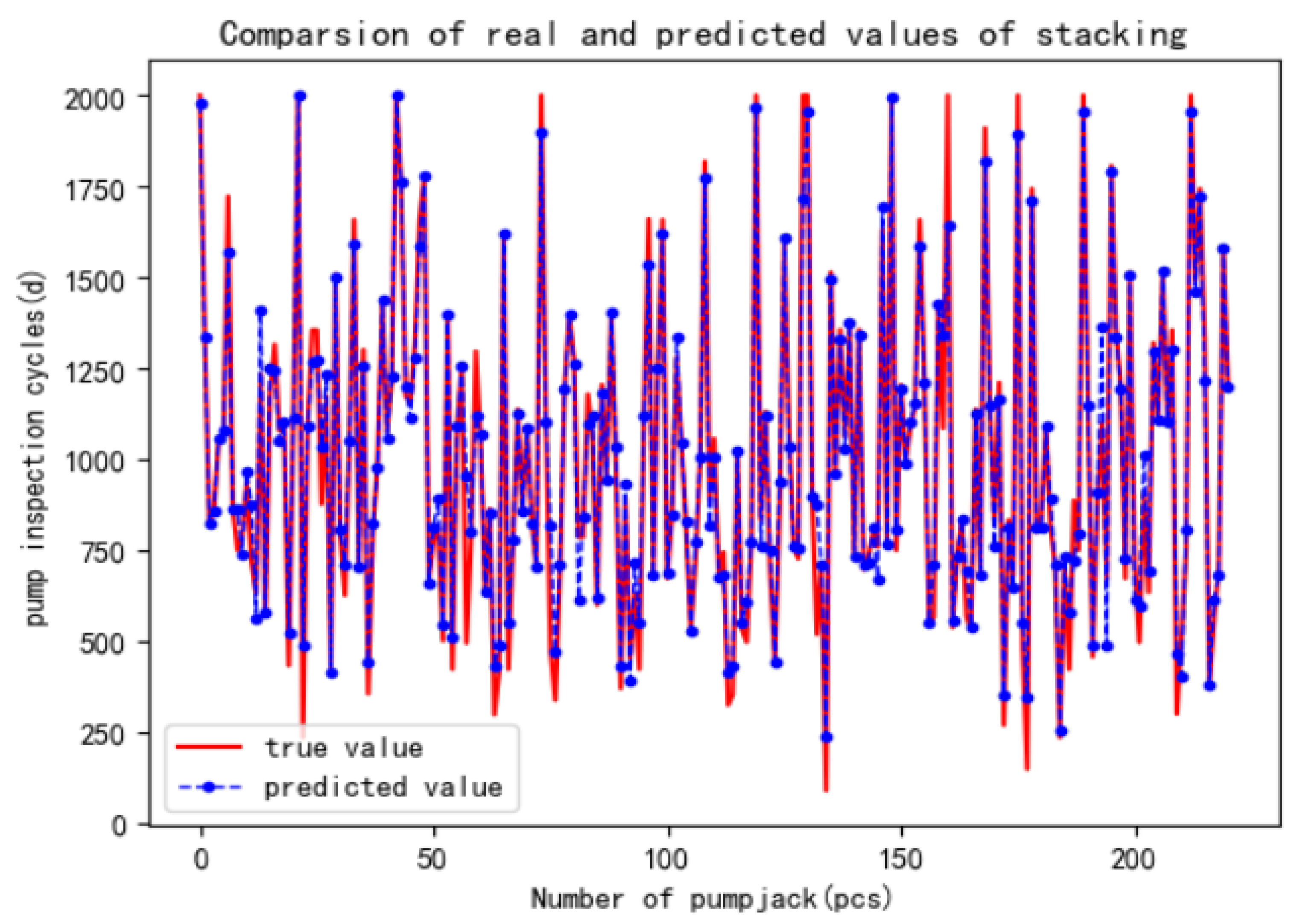
- We propose a two-layer stacking ensemble model to improve the prediction accuracy of existing methods. The first layer comprises the four models mentioned earlier, and the second layer uses ridge regression as the metalearner to prevent overfitting. Cross-training is applied to both layers. The proposed model achieves an accuracy of 92.11%, outperforming the individual model and demonstrating strong predictive capabilities.
- By calculating predicted values, we find that the pump inspection cycle’s are 427, 518, 579, 663, 705, and 964 days for the 5th, 10th, 15th, 20th, 25th, and 50th percentiles.
Author Contributions
Funding
Data Availability Statement
Conflicts of Interest
References
- Bian, Y.J.; Shi, W.; Lao, J.Y.; Chen, J.; Sun, S.L. The analysis on causes of rupture for a sucker rod made of 20CrMo alloy. Adv. Mater. Res. 2011, 295, 626–630. [Google Scholar] [CrossRef]
- Ulmanu, V.; Ghofrani, R. Fatigue life prediction method for sucker rods based on local concept; Verfahren zur Lebensdauerabschaetzung der Tiefpumpgestaenge nach dem oertlichen Konzept. Erdoel Erdgas Kohle 2001, 117, 189–195. [Google Scholar]
- Zhao, T.; Zhao, C.; He, F.; Pei, B.; Jiang, Z.; Zhou, Q. Wear analysis and safety assessment of sucker rod. China Pet. Mach. 2017, 45, 65–70. [Google Scholar]
- Dolby, J.; Shinnar, A.; Allain, A.; Reinen, J. Ariadne: Analysis for machine learning programs. In Proceedings of the 2nd ACM SIGPLAN International Workshop on Machine Learning and Programming Languages, Philadelphia, PA, USA, 18–22 June 2018; pp. 1–10. [Google Scholar]
- Hou, Y.B.; Chen, B.J.; Gao, X.W. Fault diagnosis of sucker rod pump wells based on GM-ELM. J. Northeast. Univ. (Nat. Sci.) 2019, 40, 1673. [Google Scholar]
- Deng, J.; Liu, X.; Yang, P. Research on Pump Detection Period Predicting Based on Support Vector Regression. Comput. Digit. Eng. 2023, 51, 1893–1897. [Google Scholar]
- Zhang, X.-D.; Wang, X.-Y.; Qin, Z.-X. Pump Detection Period Predicting of Pump Well Based on Feature Fusion. Comput. Mod. 2023, 12, 60–66. [Google Scholar]
- Breiman, L. Random forests. Mach. Learn. 2001, 45, 5–32. [Google Scholar] [CrossRef]
- Hastie, T.; Tibshirani, R.; Friedman, J.; Hastie, T.; Tibshirani, R.; Friedman, J. Random forests. In The Elements of Statistical Learning: Data Mining, Inference, and Prediction; Springer: Berlin/Heidelberg, Germany, 2009; pp. 587–604. [Google Scholar]
- Cutler, A.; Cutler, D.R.; Stevens, J.R. Random forests. In Ensemble Machine Learning: Methods and Applications; Springer: Berlin/Heidelberg, Germany, 2012; pp. 157–175. [Google Scholar]
- Fawagreh, K.; Gaber, M.M.; Elyan, E. Random forests: From early developments to recent advancements. Syst. Sci. Control Eng. Open Access J. 2014, 2, 602–609. [Google Scholar] [CrossRef]
- Denisko, D.; Hoffman, M.M. Classification and interaction in random forests. Proc. Natl. Acad. Sci. USA 2018, 115, 1690–1692. [Google Scholar] [CrossRef]
- Chiang, J.-Y.; Lio, Y.L.; Hsu, C.-Y.; Tsai, T.-R. Binary classification with imbalanced data. Entropy 2024, 26, 15. [Google Scholar] [CrossRef]
- Ogunleye, A.; Wang, Q.G. XGBoost model for chronic kidney disease diagnosis. IEEE/ACM Trans. Comput. Biol. Bioinform. 2019, 17, 2131–2140. [Google Scholar] [CrossRef] [PubMed]
- Chen, T.; He, T.; Benesty, M.; Khotilovich, V. Package ‘xgboost’. R Version 2019, 90, 40. [Google Scholar]
- Asselman, A.; Khaldi, M.; Aammou, S. Enhancing the prediction of student performance based on the machine learning XGBoost algorithm. Interact. Learn. Environ. 2023, 31, 3360–3379. [Google Scholar] [CrossRef]
- Li, J.; An, X.; Li, Q.; Wang, C.; Yu, H.; Zhou, X.; Geng, Y.A. Application of XGBoost algorithm in the optimization of pollutant concentration. Atmos. Res. 2022, 276, 106238. [Google Scholar] [CrossRef]
- Liu, W.; Chen, Z.; Hu, Y. XGBoost algorithm–based prediction of safety assessment for pipelines. Int. J. Press. Vessel. Pip. 2022, 197, 104655. [Google Scholar] [CrossRef]
- Ke, G.; Meng, Q.; Finley, T.; Wang, T.; Chen, W.; Ma, W.; Ye, Q.; Liu, T.-Y. Lightgbm: A highly efficient gradient boosting decision tree. Adv. Neural Inf. Process. Syst. 2017, 30, 1–9. [Google Scholar]
- Sun, X.; Liu, M.; Sima, Z. A novel cryptocurrency price trend forecasting model based on LightGBM. Financ. Res. Lett. 2022, 32, 101084. [Google Scholar] [CrossRef]
- Li, K.; Xu, H.; Liu, X. Analysis and visualization of accidents severity based on LightGBM-TPE. Chaos Solitons Fractals 2022, 157, 111987. [Google Scholar] [CrossRef]
- Yang, H.; Chen, Z.; Yang, H.; Tian, M. Predicting coronary heart disease using an improved LightGBM model: Performance analysis and comparison. IEEE Access 2023, 11, 23366–23380. [Google Scholar] [CrossRef]
- Bales, D.; Tarazaga, P.A.; Kasarda, M.; Batra, D.; Woolard, A.G.; Poston, J.D.; Malladi, V.S. Gender classification of walkers via underfloor accelerometer measurements. IEEE Internet Things J. 2016, 3, 1259–1266. [Google Scholar] [CrossRef]
- Mauldin, T.; Ngu, A.H.; Metsis, V.; Canby, M.E.; Tesic, J. Experimentation and analysis of ensemble deep learning in IoT applications. Open J. Internet Things 2019, 5, 133–149. [Google Scholar]
- Xu, H.; Yan, Z.H.; Ji, B.W.; Huang, P.F.; Cheng, J.P.; Wu, X.D. Defect detection in welding radiographic images based on semantic segmentation methods. Measurement 2022, 188, 110569. [Google Scholar] [CrossRef]
- Nafea, A.A.; Ibrahim, M.S.; Mukhlif, A.A.; AL-Ani, M.M.; Omar, N. An ensemble model for detection of adverse drug reactions. ARO-Sci. J. Koya Univ. 2024, 12, 41–47. [Google Scholar] [CrossRef]
- Terrault, N.A.; Hassanein, T.I. Management of the patient with SVR. J. Herpetol. 2016, 65, S120–S129. [Google Scholar] [CrossRef] [PubMed]
- Sun, Y.; Ding, S.; Zhang, Z.; Jia, W. An improved grid search algorithm to optimize SVR for prediction. Soft Comput. 2021, 25, 5633–5644. [Google Scholar] [CrossRef]
- Huang, J.; Sun, Y.; Zhang, J. Reduction of computational error by optimizing SVR kernel coefficients to simulate concrete compressive strength through the use of a human learning optimization algorithm. Eng. Comput. 2022, 38, 3151–3168. [Google Scholar] [CrossRef]
- Fu, X.; Zheng, Q.; Jiang, G.; Roy, K.; Huang, L.; Liu, C.; Li, K.; Chen, H.; Song, X.; Chen, J.; et al. Water quality prediction of copper-molybdenum mining-beneficiation wastewater based on the PSO-SVR model. Front. Environ. Sci. Eng. 2023, 17, 98. [Google Scholar] [CrossRef]
- Pratap, B.; Sharma, S.; Kumari, P.; Raj, S. Mechanical properties prediction of metakaolin and fly ash-based geopolymer concrete using SVR. J. Build. Pathol. Rehabil. 2024, 9, 1. [Google Scholar] [CrossRef]
- Speiser, J.L.; Miller, M.E.; Tooze, J.; Ip, E. A comparison of random forest variable selection methods for classification prediction modeling. Expert Syst. Appl. 2019, 134, 93–101. [Google Scholar] [CrossRef]
- Hegde, Y.; Padma, S.K. Sentiment analysis using random forest ensemble for mobile product reviews in Kannada. In Proceedings of the 2017 IEEE 7th International Advanced Computing Conference (IACC), Hyderabad, India, 5–7 January 2017; pp. 777–782. [Google Scholar]
- Lei, X.; Fang, Z. GBDTCDA: Predicting circRNA-disease associations based on gradient boosting decision tree with multiple biological data fusion. Int. J. Biol. Sci. 2019, 15, 2911–2924. [Google Scholar] [CrossRef]
- Wang, D.-N.; Li, L.; Zhao, D. Corporate finance risk prediction based on LightGBM. Inf. Sci. 2022, 602, 259–268. [Google Scholar] [CrossRef]
- Bao, Y.; Liu, Z. A fast grid search method in support vector regression forecasting time series. In Intelligent Data Engineering and Automated Learning–IDEAL 2006: 7th International Conference, Burgos, Spain, September 2006; Proceedings 7; Springer: Berlin/Heidelberg, Germany, 2006; pp. 504–511. [Google Scholar]
- Sabzekar, M.; Hasheminejad, S.M.H. Robust regression using support vector regressions. Chaos Solitons Fractals 2021, 144, 110738. [Google Scholar] [CrossRef]
- Allende-Cid, H.; Salas, R.; Allende, H.; Ñanculef, R. Robust alternating AdaBoost. In Progress in Pattern Recognition, Image Analysis and Applications, November, 2007; Springer: Berlin/Heidelberg, Germany, 2007; pp. 427–436. [Google Scholar]
- Wu, Y.; Ke, Y.; Chen, Z.; Liang, S.; Zhao, H.; Hong, H. Application of alternating decision tree with AdaBoost and bagging ensembles for landslide susceptibility mapping. Catena 2020, 187, 104396. [Google Scholar] [CrossRef]
- Ahmadianfar, I.; Heidari, A.A.; Noshadian, S.; Chen, H.G.; Omi, A.H. INFO: An efficient optimization algorithm based on weighted mean of vectors. Expert Syst. Appl. 2022, 195, 116516. [Google Scholar] [CrossRef]
- Fan, R.; Meng, D.; Xu, D. Survey of research process on statistical correlation analysis. Math. Model. Its Appl. 2014, 3, 1–12. [Google Scholar]
- Chemmakha, M.; Habibi, O.; Lazaar, M. Improving machine learning models for malware detection using embedded feature selection method. IFAC-PapersOnLine 2022, 55, 771–776. [Google Scholar] [CrossRef]
- Wang, G.; Fu, G.; Corcoran, C. A forest-based feature screening approach for large-scale genome data with complex structures. BMC Genet. Data 2015, 16, 148. [Google Scholar] [CrossRef]
- Yao, X.; Fu, X.; Zong, C. Short-term load forecasting method based on feature preference strategy and LightGBM-XGboost. IEEE Access 2022, 10, 75257–75268. [Google Scholar] [CrossRef]
- Yang, S.; Fountoulakis, K. Weighted flow diffusion for local graph clustering with node attributes: An algorithm and statistical guarantees. In Proceedings of the 40th International Conference on Machine Learning, Honolulu, HI, USA, 23–29 July 2023. [Google Scholar]
- Xu, K.; Chen, L.; Wang, S. Data-driven kernel subspace clustering with local manifold preservation. In Proceeding of the 2022 IEEE International Conference on Data Mining Workshops (ICDMW), Orlando, FL, USA, 28 November–1 December 2022. [Google Scholar]


| Feature Type | Production Days | The Max. Load | The Min. Load | Tubing Pressure | Casing Pressure | Daily Oil Production |
|---|---|---|---|---|---|---|
| quantity | 110 | 53 | 41 | 25 | 33 | 72 |
| Method | Parameters | Parameter Definition |
|---|---|---|
| RF | number of basic decision trees | |
| use the maximum number of fields | ||
| LightGBM | number of basic decision trees | |
| leaf count | ||
| learn rate | ||
| SVR | kernel type | |
| Penalty factor | ||
| kernel coefficient | ||
| Adaboost | random seed | |
| number of base models | ||
| learn rate |
| Method | RMSE | MAE | |
|---|---|---|---|
| RF | 2.72 | 0.98 | 90.19% |
| LightGBM | 4.31 | 2.18 | 88.77% |
| SVR | 4.77 | 1.35 | 86.16% |
| AdaBoost | 5.13 | 3.12 | 83.24% |
| Accuracy | Ridge Regression | RF | SVR |
|---|---|---|---|
| Training | 96.06% | 98.73% | 97.65% |
| Test | 91.17% | 89.61% | 89.96% |
| Methods | RMSE | MAE | |
|---|---|---|---|
| stacking | 0.73 | 0.45 | 92.11% |
| RF | 2.72 | 0.98 | 90.19% |
| LightGBM | 4.31 | 2.18 | 88.77% |
| SVR | 4.77 | 1.35 | 86.16% |
| AdaBoost | 5.13 | 3.12 | 83.24% |
Disclaimer/Publisher’s Note: The statements, opinions and data contained in all publications are solely those of the individual author(s) and contributor(s) and not of MDPI and/or the editor(s). MDPI and/or the editor(s) disclaim responsibility for any injury to people or property resulting from any ideas, methods, instructions or products referred to in the content. |
© 2024 by the authors. Licensee MDPI, Basel, Switzerland. This article is an open access article distributed under the terms and conditions of the Creative Commons Attribution (CC BY) license (https://creativecommons.org/licenses/by/4.0/).
Share and Cite
Xin, H.; Zhang, S.; Lio, Y.; Tsai, T.-R. Predicting Pump Inspection Cycles for Oil Wells Based on Stacking Ensemble Models. Mathematics 2024, 12, 2231. https://doi.org/10.3390/math12142231
Xin H, Zhang S, Lio Y, Tsai T-R. Predicting Pump Inspection Cycles for Oil Wells Based on Stacking Ensemble Models. Mathematics. 2024; 12(14):2231. https://doi.org/10.3390/math12142231
Chicago/Turabian StyleXin, Hua, Shiqi Zhang, Yuhlong Lio, and Tzong-Ru Tsai. 2024. "Predicting Pump Inspection Cycles for Oil Wells Based on Stacking Ensemble Models" Mathematics 12, no. 14: 2231. https://doi.org/10.3390/math12142231
APA StyleXin, H., Zhang, S., Lio, Y., & Tsai, T.-R. (2024). Predicting Pump Inspection Cycles for Oil Wells Based on Stacking Ensemble Models. Mathematics, 12(14), 2231. https://doi.org/10.3390/math12142231