Trajectory Tracking Control of an Autonomous Vessel in the Presence of Unknown Dynamics and Disturbances

Abstract

We present a proportional–integral–derivative-based controller plus an adaptive slide surface to solve the trajectory tracking control problem for a fully actuated vessel with unknown parameters perturbed by slowly varying external unknown dynamics. The controller design assumes that the vessel moves at low speed and frequency, its physical parameters are unknown, and its state is measurable. The control approach ensures error tracking convergence toward a small vicinity at the origin. We conduct the corresponding stability analysis using the Lyapunov theory and saturation functions. We tested the controller through two numerical experiments—a turning ellipse maneuver and a rest-to-rest maneuver—where the vessel parameters were unknown, and we obtained satisfactory results.

1. Introduction

The undesirable effects of unknown uncertainties or perturbations must be considered and counteracted in every model-based control system. For instance, aircraft and ocean vessels are the quintessential examples of models constantly affected by external perturbations due to crosswinds and ocean currents. Unfortunately, in the case of ocean vessels, even with the technology we have today, there are partially solved or unsolved complex issues that prevent us from safely and accurately carrying out tasks like dredging operations, recovery of lost human-made objects, cable laying operations, towing operations, and military operations [1,2].

Consequently, many efforts have been devoted to developing control strategies to accomplish the tasks mentioned earlier. For instance, automated or assisted tracking trajectory is often needed to perform precisely when vessels carry out maneuvers or operations in the open ocean or ports. Although, as pointed out in [3], several ocean vessels are fully actuated; they are affected by unknown perturbations to the nominal model in the form of parametric and functional uncertainties, unmodeled dynamics, and environmental disturbances. In this context, we can distinguish two cases: one when the vessels are fully actuated and one when they are underactuated [3,4,5,6]. In both cases, three control tasks arise: the tracking trajectory problem, the fixed obstacles avoidance or evasion, and dynamic positioning.

The dynamic positioning task consists of controlling the vessel position, using their thrusters and propels as actuators [7]. The most common approach found in the specialized literature, and the one we adopted in this work, considers the vessel model as a manipulator robot when moving slowly and in the presence of an unknown low-frequency, external perturbation [7,8].

The increasing interest in the ideas we mentioned earlier has led to several developments. Regarding backstepping control techniques, the work of [9] combines backstepping and Lyapunov synthesis to solve the tracking control problem for fully actuated ocean vessels in the presence of uncertainties and unknown disturbances. In [7], the authors used a vectorial observer backstepping through linearization to obtain a globally exponentially stable output feedback controller to accomplish dynamic vessel positioning. An adaptive vectorial backstepping control that requires exact knowledge of the ship’s parameters and slow time-varying disturbances is proposed in [10]. In the context of robust and adaptive control, we can mention the work of [11], where the problem of positioning marine vessels in the presence of parametric uncertainties, unknown disturbances, and input nonlinearities is addressed using a robust adaptive control with dynamic control allocation. In [12], the author constructively designed a globally robust and adaptive output feedback controller to position fully actuated vessels under environmental disturbances induced by waves, wind, and ocean currents. In [13], the trajectory tracking control problem for unmanned surface vessels with input saturation and full-state constraints is solved using the barrier Lyapunov function to handle the state constraints. At the same time, an adaptive methodology deals with unknown random disturbances and saturation problems. The work of [14] introduced a control scheme for dynamic positioning control of ships using a relay observer designed to dynamically position and maintain the vessel by exclusively using their active thrusters. A robust adaptive trajectory tracking control strategy for enhancing the tracking performance of surface vessels with unmodeled dynamics and unknown time-varying disturbances was developed in [15]. In [16], the tracking trajectory problem for unmanned surface vessels subject to input saturation and full-state constraints is addressed by using an anti-windup compensator. To solve the saturation problem, the proposed strategy achieved semi-global uniform boundedness of the closed-loop system through the Lyapunov stability theory. The trajectory tracking problem for a ship modeled as port-Hamiltonian systems is solved in [17] using a virtual contraction-based control. Sliding mode control is used in [18] to design a robust nonlinear controller for a simplified model of a six degrees of freedom fully actuated vessel. In [19], based on integral sliding mode technology, the authors developed a thruster fault tolerant control. To this end, they proposed an integral sliding mode surface and sliding mode controller with fault estimation and carried out the stability analysis using LMI technology and Lyapunov stability theory. In [20], based on the fixed-time sliding mode manifold, the authors designed a fixed-time sliding mode controller that was robust against uncertainties to track the desired trajectory of an unmanned surface vessel. This scheme ensures fixed-time position and velocity tracking errors converge to zero.

It is worth mentioning that modern artificial techniques have been successfully used for unmanned ships’ navigation. For instance, in [21], machine learning and deep learning artificial intelligence are used together with multiple sensors to accomplish a navigation approach in autonomous ships. Some authors also implement neural networks to overcome the unmodeled dynamics. That is the case in [22], where the problem of asymptotic trajectory tracking for a fully actuated marine surface vessel, subject to unmodeled dynamics and external disturbances, is solved by introducing prescribed transient performance constraints to specify the transient behavior of the output tracking errors. In [23], an exciting solution for the vessel tracking trajectory problem based on neuronal networks, combined with a sliding mode version and the adaptive control law, is introduced. The neuronal network counteracts the undesirable disturbance effect in this approach, while the sliding mode and the adaptive controller improve the robustness approach.

A full review of the existing literature dealing with the tracking trajectory problem for fully actuated vessels is beyond the scope of this study; therefore, we invite the interested reader to see the references found in the cited works. The underactuated case is not less attractive nor less challenging than the fully actuated with uncertainties instance, which we are dealing with here. However, we do not review the corresponding literature; instead, we suggest to the engaging reader the work [3] and the references therein. It is worth mentioning that in the case of the tracking trajectory problem, the above revised control solutions have different assumptions; for instance, one solution needs an inertia matrix average estimation, another has to measure the whole system state, while others have several fixed or adaptable parameters, or the external perturbations must be continuous and derivable. In this context, a performance comparative analysis is a challenging task beyond the scope of this study.

This study presents a solution for the trajectory tracking control problem for a fully actuated vessel that moves at low speed and frequency. The vessel’s parameters are unknown, and its state is available for measurements. To solve this control problem, we used a nonlinear PID controller and an adaptive sliding surface, allowing us to design an adaptive control law that does not require knowledge of the vessel’s physical parameters. This control law ensures that tracking error converges toward a small vicinity at the origin. We performed the stability analysis using the Lyapunov method and numerically tested our controller’s effectiveness. We organize the remainder of this study as follows. In Section 2, we introduce the problem statement and the design of our control strategy. We developed the numerical experiments in Section 3, while we present the conclusions in Section 4.

Notation: 

In what follows, we use the following notation:

• The symbol $\mathrm{sign}\left[x\right]$, with $x\in \Re$, refers to the sign function of a real number and is defined as

  $$\mathrm{sign}\left[x\right]:=\left\{\begin{array}{cc}1\hfill & \mathrm{if}x>0\hfill \\ -1\hfill & \mathrm{if}x<0\hfill \\ \in [-1,1]\hfill & \mathrm{if}x=0\hfill \end{array}.\right.$$
• The symbol $\mathrm{sign}\left[y\right]$, with $y\in {\Re }^n$, refers to the sign function of a vector of real numbers and is defined as

$$\mathrm{sign}\left[y\right]={\left[\begin{array}{ccc}\mathrm{sign}\left[y_1\right]& \dots & \mathrm{sign}\left[y_n\right]\end{array}\right]}^T.$$

• The symbol $\sigma \left[x\right]$, with $x\in \Re$, refers to the linear saturation function defined as

  $$\sigma \left[x\right]=\left\{x \mathrm{if} \left|x\right|<1; \mathrm{else}; \mathrm{sign}\left[x\right]\right\}.$$
• In similar form $\sigma \left[y\right]$, with $y\in {\Re }^n$, refers to the vector of linear saturation function defined as

$$\sigma \left[y\right]={\left[\begin{array}{ccc}\sigma \left[y_1\right]& \dots & \sigma \left[y_n\right]\end{array}\right]}^T.$$

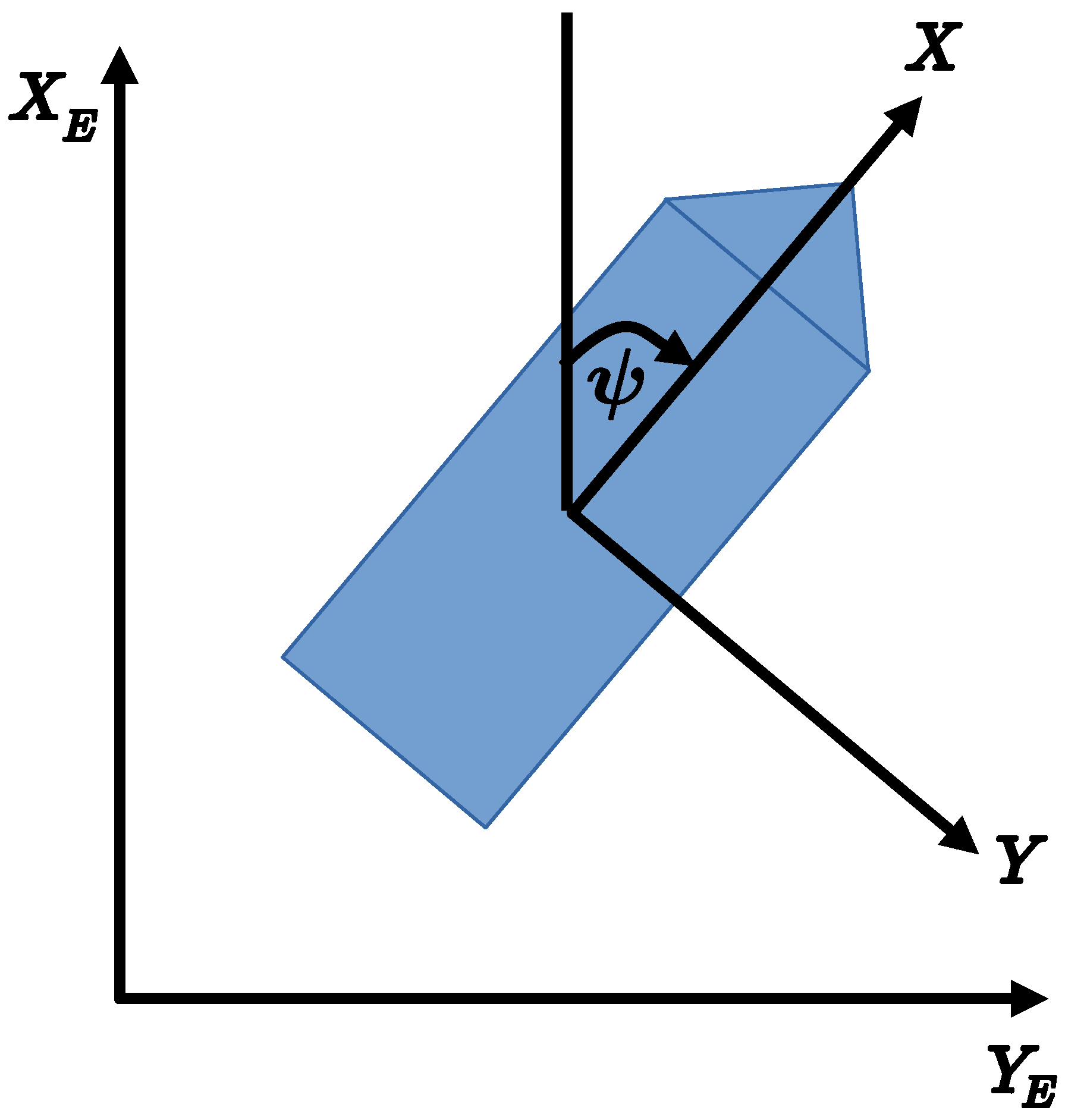
2. Dynamic Model and Problem Statement

The mathematical model for the fully actuated vessel [8,12,14], shown in Figure 1, is assumed to have the following form:

$$M\stackrel{.}{v}+Dv=\tau +d_E(t,\eta ,v),$$

(1)

$$\stackrel{.}{\eta }=R\left(\psi \right)v,$$

(2)

where $\eta ={\left[x,y,\psi \right]}^T\in {\Re }^3$ is the system state. The variables x and y denote the translational vessel position, the variable $\psi$ denotes the yaw angle relative to an Earth-fixed coordinate frame $\{X_e, Y_e\}$, v is the vessel velocity relative to the body-fixed coordinate frame $\{X_b, Y_b\}$, and $d_E(\ast )\in {\Re }^3$ is the unknown environment disturbance or unmodeled dynamics; $\tau \in {\Re }^3$ is a control vector of forces and moment provided by the propulsion system that is the vessel’s main propellers shaft and thrusters, which can produce surge and sway forces, as well as a yaw moment. The constant, positive definite, symmetric, mass–inertia matrix is $M\in {\Re }^{3\times 3}$, $D\in {\Re }^{3\times 3}$ is the constant damping matrix, and $R\left(\psi \right)\in {\Re }^{3\times 3}$ is the rotation matrix between the Earth- and body-fixed coordinate frames. The above-defined matrices can be explicitly given by

$$\begin{array}{ccc}M=\left[\begin{array}{ccc}{m}_{11}& 0& 0\\ 0& m_{22}& m_{23}\\ 0& m_{23}& m_{33}\end{array}\right],& & D=\left[\begin{array}{ccc}{d}_{11}& 0& 0\\ 0& d_{22}& d_{23}\\ 0& d_{32}& d_{33}\end{array}\right],\end{array}$$

and

$$R\left(\psi \right)=\left[\begin{array}{ccc}cos\psi & -sin\psi & 0\\ sin\psi & cos\psi & 0\\ 0& 0& 1\end{array}\right].$$

Notice that $R^{-1}\left(\psi \right)=R^T\left(\psi \right)$ is a rotational matrix with respect to the z-axis.

In our control application, the vessel movements and displacements are restricted to low-frequency moves and low velocities. Therefore, the eigenvalues of the damping matrix D are positive, and evidently, $\stackrel{.}{M}=0$ [14]. Please note that the dynamical model in (1) and (2) can be expressed as if it were a robot manipulator. To this end, we differentiate (2) and using (1), to obtain

$$\stackrel{..}{\eta }=\stackrel{.}{R}\left(\psi \right)v+R\left(\psi \right)M^{-1}\left(-Dv+\tau +d_E(t, \eta , v)\right).$$

Now, substituting the identity $R^T\left(\psi \right)\stackrel{.}{\eta }=v$, we obtain

$$\stackrel{..}{\eta }=\stackrel{.}{R}\left(\psi \right)R^T\left(\psi \right)\stackrel{.}{\eta }+R\left(\psi \right)M^{-1}\left(-D{R}^T\left(\psi \right)\stackrel{.}{\eta }+\tau +d_E(t, \eta , v)\right).$$

Multiplying the above equation for $R\left(\psi \right)M{R}^T\left(\psi \right)$ and using the identity $\stackrel{.}{R}\left(\psi \right)R^T\left(\psi \right)=R\left(\psi \right)\stackrel{.}{R}\left(\psi \right)$, we obtain

$$J\left(\eta \right)\stackrel{..}{\eta }+C(\eta ,\stackrel{.}{\eta })\stackrel{.}{\eta }+F\left(\eta \right)\stackrel{.}{\eta }={\tau }_n+\delta ,$$

(3)

where

$$\begin{array}{ccc}J\left(\eta \right)=RM{R}^T& ,& C(\eta ,\stackrel{.}{\eta })=RM\stackrel{.}{R},\\ F\left(\eta \right)=RD{R}^T& ,& \begin{array}{ccc}{\tau }_n=R\tau & ,& \delta =R{d}_E(\ast ),\end{array}\end{array}$$

with the low-frequency disturbance $\delta$ bounded. The explicit expressions from the above equalities can be found in [24]. The properties of the model Equation (3), which are similar to the classical robot dynamics [25], are the following:

Property 1:

The mass–inertia matrix $J\left(\eta \right)$ is symmetric and positive definite, i.e.,

$$\begin{array}{ccc}{j}_L{∥u∥}^2\le u^{T}J\left(\eta \right)u\le j_M{∥u∥}^2& ,& \forall u\in {\Re }^3,\end{array}$$

where $j_L$ and $j_M$ are strictly positive constants.

Property 2:

The matrices $J\left(\eta \right)$ and $C(\eta ,\stackrel{.}{\eta })$ fulfill the following skew-symmetric relationship:

$$\begin{array}{ccc}{u}^T\left(\stackrel{.}{J}\left(\eta \right)-2C(\eta ,\stackrel{.}{\eta })\right)u=0& ;& \forall u\in {\Re }^3.\end{array}$$

Please note that the manipulator robot has been extensively studied, and several controller solutions have been formulated. Evidently, a full review of these solutions and a comparison with our proposal is beyond the scope of this study (we suggest to the interested reader the book [26], and the references therein).

Before writing the control problem statement, we introduce the following useful and needed assumptions:

(A1)

The perturbation $d_E(\ast )$ satisfies

$$∥d_E(\ast )∥\le {\delta }_0,$$

(4)

where ${\delta }_0>0$ is an unknown parameter.

(A2)

the state variables $\eta$ and $\stackrel{.}{\eta }$ are measurable.

Control problem: 

Under assumptions A1 and A2, consider the almost unknown vessel system (3). The control task involves ensuring that the output $\eta$ follows the desired trajectory ${\eta }_d$, such that the tracking errors

$$\begin{array}{cc}∥\eta -{\eta }_d∥\le ϵ,& ∥\stackrel{.}{\eta }-{\stackrel{.}{\eta }}_d∥\le ϵ;\forall \hspace{1em}t\ge T_0>0\end{array},$$

where $ϵ>0$ is as small as desired, $t\ge T_0>0$ with constant $T_0$ is the time when the states enter into a confinement region, and ${\eta }_d$ is continuous and smooth, with its first and second time derivatives bounded.

Limitations

We must point out that $\eta$, its corresponding velocity $\stackrel{.}{\eta }$, and the input ${\tau }_n$ are measurable. That is, we need to feed back the velocity; if not available, we can estimate it using, for instance, an extended-order observer [27,28], a super twisting observer [29,30,31], or an extended Kalman filter [32]. In real life, our controller can be realizable because regulations require that vessels possess dead reckoning capabilities, which is the process of estimating position relative. The inertial navigation systems use dead reckoning to deduct position, velocity, and attitude [33]; then, we can assume that the whole state is available, allowing us to implement our controller. Finally, we do not know the values of matrices $M>0$ and $D>0$. In other words, $J\left(\eta \right)$, $C(\eta ,\stackrel{.}{\eta })$, and $F\left(\eta \right)$ are unknown.

3. Control Strategy

In this section, inspired by [34,35], we present the controller to solve the trajectory tracking problem for the perturbed uncertain vessel model (3). This controller guarantees tracking error convergence to a small neighborhood of zero in finite time, even when all vessel physical parameters and perturbations are unknown. To this end, we introduce the following auxiliary lemma necessary for a particular second-order uncertain system and use it to propose the stabilizing controller for the vessel model (3).

Motivation:

 

Consider the uncertain second-order system defined by

$$\begin{array}{c}{\stackrel{.}{x}}_1=x_2\hfill \\ {\stackrel{.}{x}}_2=u+d(x,t),\hfill \end{array}$$

(5)

where $x=\left[x_1,x_2\right]$ and d is an uncertainty containing unknown dynamics and disturbances, and satisfies the following:

$$\left|d(x,t)\right|\le \alpha \left(x\right)K^{\ast },$$

(6)

where $\alpha$ is a strictly positive continuous known function and $K^{\ast }$ is a strictly positive unknown positive constant. Suppose we want to practically solve the system’s trajectory tracking problem (5), assuming that x and u are measurable. To this end, we define the following auxiliary variable:

$$s=\lambda (x_1-x_r)+(x_2-{\stackrel{.}{x}}_r)=\lambda e+\stackrel{.}{e},$$

(7)

where $\lambda \in {\Re }_{+}$ and $x_r$ and ${\stackrel{.}{x}}_r$ are continuous and smooth references. Evidently, from the relation (7), if $s\to 0$, the error e exponentially converges to zero. Then, the main goal involves accomplishing $\left|s\right|<ϵ$ with $ϵ$ as small as possible. To do this, we proceed to derive the signal (7) obtaining

$$\stackrel{.}{s}=\lambda \stackrel{.}{e}+u+d(x,t)-{\stackrel{..}{x}}_r.$$

(8)

Based on relations (6) and (8) and the guidelines suggested in [34,35], we propose the following dynamical controller:

$$\begin{array}{c}u={\stackrel{..}{x}}_r-\lambda \stackrel{.}{e}-\alpha \left(x\right)\widehat{K}\mathrm{sign}\left[s\right]-k_I\sigma \left[z\right]-k_p\mathrm{sign}\left[s\right]{\left|s\right|}^{\rho }\hfill \\ \stackrel{.}{z}=s-\kappa z\hfill \\ \stackrel{.}{\widehat{K}}=\alpha \left(x\right)\left|s\right|-\beta \widehat{K},\hfill \end{array}$$

(9)

with $0<\rho \le 1$, the set of constants $\{k_P, k_I, \kappa , \beta \}\in {\Re }_{+}$, and $\widehat{K}$ is the adaptive gain, selected such that $\widehat{K}\left(0\right)>0$. Now, we develop the corresponding stability analysis of (8) in closed loop with (9), through the globally uniformly ultimately bounded (GUUB) solutions notion. To this end, we introduce the following proposition:

Proposition 1.

The uncertain system (5), in closed loop with (9), is GUUB, with its corresponding bound given by

$$\left|s\left(t\right)\right|\le {\left({\displaystyle \frac{ϵ}{k_p}}\right)}^{{\displaystyle \frac{1}{\rho +1}}}$$

and the tracking error fulfills

$$\left|e\left(t\right)\right|\le {\displaystyle \frac{1}{\lambda }}{\left({\displaystyle \frac{ϵ}{k_p}}\right)}^{{\displaystyle \frac{1}{\rho +1}}}$$

for all $t>t_0$, where $t_0$ is the instant when the system enters into the confinement region and $ϵ=\beta K^{\ast }/2$.

Proof. 

Substituting (9) into (8), we obtain

$$\begin{array}{c}\stackrel{.}{s}=-\alpha \left(x\right)\widehat{K}\mathrm{sign}\left[s\right]-k_I\sigma \left[z\right]-k_p\mathrm{sign}\left[s\right]{\left|s\right|}^{\rho }+d(x,t),\hfill \\ \stackrel{.}{z}=s-\kappa z,\hfill \\ \stackrel{.}{\widehat{K}}=\alpha \left(x\right)\left|s\right|-\beta \widehat{K}.\hfill \end{array}$$

(10)

Because $\widehat{K}\left(0\right)>0$, then we can claim that $\widehat{K}\left(t\right)>0$ for all $t\ge 0$; that is, $\widehat{K}$ is always positive. Now, to perform the convergence analysis, we use the following Lyapunov candidate function:

$$V={\displaystyle \frac{1}{2}}{s}^2+k_I{\int }_0^z\sigma \left[s\right]ds+{\displaystyle \frac{1}{2}}{\left(\widehat{K}-K^{\ast }\right)}^2.$$

(11)

Notice that function V is definite positive and radially bounded. Hence, computing the time derivative of (11) around the trajectories of systems (10), leads to

$$\stackrel{.}{V}=-k_p{\left|s\right|}^{\rho +1}-\alpha \left(x\right)\widehat{K}\left|s\right|+d\left(t\right)s-k_I\kappa z\sigma \left[z\right]+\left(\widehat{K}-K^{\ast }\right)\left(\alpha \left(x\right)\left|s\right|-\beta \widehat{K}\right).$$

Using the relation (6), it is easy to see that the equation above can be upper bounded by

$$\stackrel{.}{V}\le -k_p{\left|s\right|}^{\rho +1}-k_I\kappa z\sigma \left[z\right]-\beta \left(\widehat{K}-K^{\ast }\right)\widehat{K}.$$

(12)

Even when $\stackrel{.}{V}$ is not always less than or equal to zero, this function allows us to ensure that the states are ultimately bounded. To probe the latter, we use the following identity:

$$K^{\ast }\widehat{K}-{\widehat{K}}^2=-{\left({\displaystyle \frac{\widehat{K}}{\sqrt{2}}}-{\displaystyle \frac{K^{\ast }}{\sqrt{2}}}\right)}^2-{\displaystyle \frac{{\widehat{K}}^2}{2}}+{\displaystyle \frac{K^{\ast 2}}{2}}.$$

(13)

Substituting this identity in (12), we obtain the following:

$$\stackrel{.}{V}\le -k_p{\left|s\right|}^{\rho +1}-k_I\kappa z\sigma \left[z\right]-{\displaystyle \frac{1}{2}}\beta {\left(\widehat{K}-K^{\ast }\right)}^2+ϵ,$$

(14)

where $ϵ=\beta K^{\ast 2}/2$. From the above, we can conclude that $\stackrel{.}{V}<ϵ$ holds. From this fact, we can conclude that the states s, z, and $\widehat{K}$ cannot have a finite time of escape [36]. Therefore, in a finite time interval, all the states are bounded. To find the bounds, we proceed as follows: once again, from the inequality (12), we have that $\stackrel{.}{V}$ is strictly decreasing as long as $\widehat{K}-K^{\ast }>0$ because, as already mentioned, the state $\widehat{K}$ is always positive. Then, there exists a finite time $t_0>0$ such that

$$0<\widehat{K}\left(t\right)\le K^{\ast }<\infty ,\forall t\ge t_0>0.$$

That is, the state $\widehat{K}$ is bounded. To find the bounds of s and z, we must note that, according to inequality (14), $\stackrel{.}{V}<0$ as long as $k_p{\left|s\right|}^{\rho +1}>ϵ$. That this, there is a finite time $t_1>0$, such that

$$\left|s\left(t\right)\right|\le {ϵ}_{\ast }={\left({\displaystyle \frac{ϵ}{k_p}}\right)}^{{\displaystyle \frac{1}{\rho +1}}};\forall t\ge t_1>0.$$

(15)

Then, we can conclude that the confined region of the variable s can be reduced by selecting $\beta$ small enough and $k_P$ large enough. Developing a similar analysis as before, we can ensure that there exists a time $t_2>0$, such that

$$\left|z\right|<max\left\{{\displaystyle \frac{ϵ}{k_I}},\sqrt{{\displaystyle \frac{ϵ}{k_I}}}\right\}.$$

In conclusion, we can say that all the states are bounded, and the confined region of s can be small enough, selecting $k_p$ sufficiently large and $\beta$ sufficiently small. Even more, it is possible that in the limit, when $\beta \to 0$, then $s\to 0$. However, we must be careful if $\beta =0$, because $\widehat{K}$ can grow a lot and the third equation of (10) reads as

$$\stackrel{.}{\widehat{K}}=\alpha \left(x\right)\left|s\right|;\widehat{K}\left(0\right)>0.$$

Evidently, $\stackrel{.}{\widehat{K}}=0\iff s=0$, but we can only ensure this implication when $t\to \infty$. A way to avoid $\widehat{K}$ growing a lot consists of proposing $\stackrel{.}{\widehat{K}}$ as follows:

$$\stackrel{.}{\widehat{K}}=\left\{\begin{array}{c}\alpha \left(x\right)\left|s\right|,\hspace{1em}\hspace{1em}\mathrm{if}\left|s\right|>ϵ,\hfill \\ 0,\hspace{1em}\hspace{1em}\hspace{1em}\hspace{1em}\mathrm{if}\left|s\right|\le ϵ\hfill \end{array}\right.,$$

with $ϵ$ sufficiently small and $\widehat{K}\left(0\right)>0$.

Finally, we must underscore that if $\kappa =0$ and $\rho =1$, and we use ${\sigma }_M\left[z\right]=z$ with M sufficiently large, we have that the controller (9) can be implemented as

$$\begin{array}{c}u=-\alpha \left(x\right)\widehat{K}\mathrm{sign}\left[s\right]-k_I{\int }_0^{t}z\left(s\right)ds-k_{p}s,\hfill \\ \stackrel{.}{\widehat{K}}=\alpha \left(x\right)\left|s\right|-\beta \widehat{K}.\hfill \end{array}$$

The last system of equations shows that the integral action counteracts the low-frequency uncertainties’ undesirable effect, allowing us to reduce the gain size $\widehat{K}$. □

The proposed control law (9) can be substituted by the following control:

$$u=-\lambda \stackrel{.}{e}-\alpha \left(x\right)\widehat{K}\mathrm{sign}\left[s\right]-k_I\sigma \left[z\right]-k_p\sigma \left[s\right],$$

(16)

which, in closed loop with (5), converts to

$$\begin{array}{c}\stackrel{.}{s}=-\alpha \left(x\right)\widehat{K}\mathrm{sign}\left[s\right]-k_I\sigma \left[z\right]-k_p\sigma \left[s\right]+\tilde{d}(x,t),\hfill \\ \stackrel{.}{z}=s-\kappa z,\hfill \\ \stackrel{.}{\widehat{K}}=\alpha \left(x\right)\left|s\right|-\beta \widehat{K},\hfill \end{array}$$

(17)

where $\tilde{d}(x,t)=d(x,t)+{\stackrel{.}{x}}_r$. Using the above introduced Lyapunov function (11) and its time derivative around the trajectories of (17), it is possible to show that $\stackrel{.}{V}$ can be upper bounded as follows:

$$\stackrel{.}{V}\le -k_{p}s\sigma \left[s\right]-k_I\kappa z\sigma \left[z\right]-{\displaystyle \frac{1}{2}}\beta {\left(\widehat{K}-K^{\ast }\right)}^2+ϵ.$$

Once again, using the previous discussion, we can show that all the states are bounded, and s can be bounded as

$$\left|s\right|<max\left\{{\displaystyle \frac{ϵ}{k_p}},\sqrt{{\displaystyle \frac{ϵ}{kp}}}\right\}.$$

Now, we proceed to estimate the tracking trajectory behavior. Furthermore, the saturation function in the controller (16) can be substituted by any smooth saturation function; for instance, $\sigma \left[z\right]=tanh\left(z\right)$.

Tracking trajectory error behavior: 

from the definitions of s given in (7) and the tracking error $e=x_1-x_r$, we have that the equality (15) can be written as

$$-{ϵ}_{\ast }\le \lambda e\left(t\right)+\stackrel{.}{e}\left(t\right)\le {ϵ}_{\ast }$$

(18)

for all $t\ge$$t_0$. Then, if we multiply (18) by exp$\left(\lambda t\right)$, after some simple algebra, we have

$$-{ϵ}_{\ast }exp\left(\lambda t\right)\le {\displaystyle \frac{d}{dt}}\left[exp\left(\lambda t\right)e\left(t\right)\right]\le {ϵ}_{\ast }exp\left(\lambda t\right).$$

Integrating the above inequality as follows:

$$-{ϵ}_{\ast }{\int }_{t_0}^{t}exp\left(\lambda \tau \right)d\tau \le {\int }_{t_0}^t{\displaystyle \frac{d}{dt}}\left[exp\left(\lambda \tau \right)e\left(\tau \right)\right]d\tau \le {ϵ}_{\ast }{\int }_{t_0}^{t}exp\left(\lambda \tau \right)d\tau ,$$

we have

$$\left|e\left(t\right)\right|\le e\left(t_0\right)exp\left(-\lambda (t-t_0)\right)+{\displaystyle \frac{{ϵ}_{\ast }}{\lambda }}\left(1-exp\left(-\lambda \left(t-t_0\right)\right)\right),$$

which implies that

$$\left|e\left(t\right)\right|\le {\displaystyle \frac{{ϵ}_{\ast }}{\lambda }}$$

for $t>>t_0$. That is, we can reduce $e\left(t\right)$ by selecting $\beta$ small and $\lambda$ and $k_P$ sufficiently large.

The Trajectory Control Law for the Vessel

In this section, we apply Proposition 1 to control the model (3). To this end, we consider that the desired trajectories ${\eta }_d$, ${\stackrel{.}{\eta }}_d$, and ${\stackrel{..}{\eta }}_d\in {\Re }^3$ are bounded. Let us now define the tracking error as $e_T=\eta -{\eta }_d\in {\Re }^3$. Once again, we define the auxiliary variable $s\in {\Re }^3$ as

$$s={\stackrel{.}{e}}_T+\mathsf{\Lambda }{e}_T,$$

(19)

where $\mathsf{\Lambda }=diag\{{\lambda }_1,{\lambda }_2,{\lambda }_3\}$ is positive definite. Then, we want that $∥s\left(t\right)∥\le {ϵ}_k$ holds for all $t\ge t_0>0$, where ${ϵ}_k$ is as small as we desire. Once again, if $s=0$, then tracking trajectory error $e_T$ exponentially converges to zero. To this end, we use the above definition of the slide surface (19) and the definition of Equation (3), and we can see that the relation holds as follows:

$$J\left(\eta \right)\stackrel{.}{s}=J\left(\eta \right)\left(\stackrel{..}{\eta }-{\stackrel{..}{\eta }}_d+\mathsf{\Lambda }{\stackrel{.}{e}}_T\right)={\tau }_n-Cs+\overline{\delta }(t,\eta ,\stackrel{.}{\eta }),$$

(20)

where

$$\overline{\delta }(t,\eta ,\stackrel{.}{\eta })=-\left(C\stackrel{.}{\eta }+F\left(\eta \right)\stackrel{.}{\eta }+\delta (t,\eta ,\stackrel{.}{\eta })+J\left(\eta \right){\stackrel{..}{\eta }}_d-J\left(\eta \right)\mathsf{\Lambda }{\stackrel{.}{e}}_T-Cs\right).$$

Using simple algebra, we can show that $\overline{\delta }(\ast )$ can be upper bounded as

$$∥\overline{\delta }∥\le K_0^{\ast }+K_1^{\ast }∥\vartheta ∥+K_2^{\ast }{∥\vartheta ∥}^2,$$

(21)

where $\vartheta =\left[\eta ,\stackrel{.}{\eta }\right]$ and $K_i^{\ast }(i\in \{0,1,2\})$ are unknown suitable constants. For more details on the last inequality, see Appendix A.

After introducing the needed foundations, we are in a condition to solve the main goal of this study. To this end, following the line of Proposition 1 and the inequality (21), we propose

$$\begin{array}{c}{\tau }_n=-k_p{\left[s\right]}^{\rho }-\mathrm{sign}\left(s\right)\sum _{i=0}^2{\widehat{K}}_i{∥\vartheta ∥}^i-k_I\sigma \left[z\right]\hfill \\ \stackrel{.}{z}=s-\kappa z\hfill \end{array},$$

(22)

where the symbol ${\left[s\right]}^{\rho }$ means ${\left[s\right]}^{\rho }={[\mathrm{sign}\left(s_1\right){\left|s_1\right|}^{\rho },\mathrm{sign}\left(s_2\right){\left|s_2\right|}^{\rho },\mathrm{sign}\left(s_3\right){\left|s_3\right|}^{\rho }]}^T;$$k_p$, $k_I$, $\kappa \in {\Re }_{+}$, s and $z\in {\Re }^3$, and the adaptive gains ${\widehat{K}}_i$ evolve according to the following equations:

$$\begin{array}{c}{\stackrel{.}{\widehat{K}}}_i=∥s∥{∥\vartheta ∥}^i-{\beta }_i{\widehat{K}}_i,\hfill \\ {\widehat{K}}_i\left(0\right)>0,\hspace{1em}{\beta }_i>0,\hspace{1em}i\in \{0, 1, 2\},\hfill \end{array}$$

(23)

where ${\beta }_i$ are design constants.

Now, we proceed to carry out a stability analysis of the vessel system in a closed loop with (22) and (23), which is the main result of this study. To this end, we introduce the main proposition:

Proposition 2.

Under Properties 1 and 2, the control system (3), in closed loop with (22) and the adaptive control gains (23), make the vessel system a GUUB with the ultimate bound s given by

$$∥s\left(t\right)∥\le \underline{ϵ}=\sqrt{{\displaystyle \frac{1}{k_1}}\sum _{i=0}^2{\displaystyle \frac{{\beta }_i{K}_i^{\ast 2}}{2}}}$$

for all $t\ge t_0$, where $t_0$ is the instant when the system enters into the confinement region. Furthermore, in steady state, the tracking trajectory error satisfies

$$\left|e_{T_i}\left(t\right)\right|\le {\displaystyle \frac{{\underline{ϵ}}^{\frac{1}{\rho +1}}}{{\lambda }_i}};\hspace{1em}i\in \{1, 2, 3\}.$$

Proof. 

According to relations in (23), we can evidently claim that ${\widehat{K}}_i\left(t\right)>0$ for all $t\ge 0$ and $i\in \{0, 1, 2\}$.

To carry out the closed-loop stability, we use the following Lyapunov candidate function:

$$V={\displaystyle \frac{1}{2}}{s}^{T}J\left(\eta \right)s+k_I\sum _{i=1}^3{\int }_0^{z_i}\sigma \left[{\tau }_i\right]d{\tau }_i+{\displaystyle \frac{1}{2}}\sum _{i=0}^2{\left({\widehat{K}}_i-K_i^{\ast }\right)}^2.$$

(24)

Now, the time derivative of (24) is given by

$$\stackrel{.}{V}=s^{T}J\left(\eta \right)\stackrel{.}{s}+{\displaystyle \frac{s^T\stackrel{.}{J}\left(\eta \right)s}{2}}+k_I\sum _{i=1}^3\sigma \left[z_i\right]{\stackrel{.}{z}}_i+\sum _{i=0}^2\left({\widehat{K}}_i-K_i^{\ast }\right){\stackrel{.}{\widehat{K}}}_i.$$

(25)

Substituting (20) and (22) into (25), we obtain

$$\begin{array}{cc}\stackrel{.}{V}=\hfill & s^T\left({\tau }_n+\overline{\delta }(\ast )\right)+s^T\left(-C+{\displaystyle \frac{\stackrel{.}{J}\left(\eta \right)}{2}}\right)s\hfill \\ \hfill & +k_I\sum _{i=1}^3\sigma \left[z_i\right]{\stackrel{.}{z}}_i+\sum _{i=0}^2\left({\widehat{K}}_i-K_i^{\ast }\right){\stackrel{.}{\widehat{K}}}_i.\hfill \end{array}$$

Using Property 2, the second equation of (22), and (23), we have that the above equation can be upper bounded as

$$\begin{array}{cc}\stackrel{.}{V}\hfill & \le -\sum _{i=1}^3\left(k_p{\left|s_i\right|}^{\rho +1}+\kappa k_I\sigma \left[z_i\right]z_i\right)-∥s∥\sum _{i=0}^2{\widehat{K}}_i{∥\vartheta ∥}^i\hfill \\ \hfill & +\sum _{i=0}^2∥s∥K_i^{\ast }{∥\vartheta ∥}^i+\sum _{i=0}^2\left({\widehat{K}}_i-K_i^{\ast }\right)\left(∥s∥{∥\vartheta ∥}^i-{\beta }_i{\widehat{K}}_i\right),\hfill \end{array}$$

which can be algebraically reduced as

$$\stackrel{.}{V}\le -\sum _{i=1}^3\left(k_p{\left|s_i\right|}^{\rho +1}+\kappa k_I\sigma \left[z_i\right]z_i\right)-\sum _{i=0}^2\left({\widehat{K}}_i-K_i^{\ast }\right){\beta }_i{\widehat{K}}_i.$$

(26)

Now, substituting the following equality

$$K_i^{\ast }{\widehat{K}}_i-{\widehat{K}}_i^2=-{\left({\displaystyle \frac{{\widehat{K}}_i}{\sqrt{2}}}-{\displaystyle \frac{K_i^{\ast }}{\sqrt{2}}}\right)}^2-{\displaystyle \frac{{\widehat{K}}_i^2}{2}}+{\displaystyle \frac{K_i^{\ast 2}}{2}}$$

into the inequality (26), we obtain the following:

$$\begin{array}{cc}\stackrel{.}{V}\le \hfill & -\sum _{i=1}^3\left(k_p{\left|s_i\right|}^{\rho +1}+\kappa k_I\sigma \left[z_i\right]z_i\right)-\sum _{i=0}^2{\beta }_i{\left({\displaystyle \frac{{\widehat{K}}_i}{\sqrt{2}}}-{\displaystyle \frac{K_i^{\ast }}{\sqrt{2}}}\right)}^2\hfill \\ \hfill & +\sum _{i=0}^2{\beta }_i{\displaystyle \frac{K_i^{\ast 2}}{2}}.\hfill \end{array}$$

(27)

Using the previous arguments verbatim, we can conclude that the states s, z, and ${\widehat{K}}_i$ with $i\in \{0, 1, 2\}$ are bounded for a certain time $t_0>0$. To find a confinement bound for signal s, we proceed as follows. From (27), we can see that $\stackrel{.}{V}$ is strictly negative as long as

$$k_p\sum _{i=1}^3{\left|s_i\right|}^{\rho +1}>\sum _{i=0}^2{\beta }_i{\displaystyle \frac{K_i^{\ast 2}}{2}}.$$

Therefore, there exists a finite time $t_1>0$, such that the inequality holds as follows:

$$\sum _{i=1}^3{\left|s_i\left(t\right)\right|}^{\rho +1}\le \underline{ϵ}={\displaystyle \frac{1}{k_p}}\sum _{i=0}^2{\beta }_i{\displaystyle \frac{K_i^{\ast 2}}{2}};\hspace{1em}\hspace{1em}\forall t\ge t_1.$$

(28)

That is to say, the confinement region for variable s is computed as

$$\left|s_i\left(t\right)\right|\le ∥s\left(t\right)∥\le {\underline{ϵ}}^{{\displaystyle \frac{1}{\rho +1}}};\hspace{1em}\hspace{1em}i\in \{1,2,3\}\hspace{1em}\hspace{1em}and\hspace{1em}\hspace{1em}\forall t\ge t_0.$$

(29)

Notice that, to make the confinement region of $s_i$ with $i\in \{1, 2, 3\}$ very small, we need to select $k_p$ sufficiently large and ${\beta }_i$ with $i\in \{1, 2, 3\}$ sufficiently small. After having computed the error of variable s, we can estimate the tracking error $e_T=[e_{T_1},e_{T_2},e_{T_3}]$. From the definition of s given in (19) and the inequality (29), we have

$$-{\underline{ϵ}}^{{\displaystyle \frac{1}{\rho +1}}}\le \stackrel{s_i\left(t\right)}{\overbrace{{\lambda }_i{e}_{T_i}\left(t\right)+{\stackrel{.}{e}}_{T_i}\left(t\right)}}\le {\underline{ϵ}}^{{\displaystyle \frac{1}{\rho +1}}};\hspace{1em}\hspace{1em}i\in \{1, 2, 3\}$$

for all $t\ge t_0>0$. Mimicking the steps in the subsection Tracking trajectory error behavior, we can conclude that

$$\left|e_{T_i}\left(t\right)\right|\le {\displaystyle \frac{{\underline{ϵ}}^{\frac{1}{\rho +1}}}{{\lambda }_i}};\hspace{1em}\hspace{1em}i\in \{1, 2, 3\},$$

and for all $t>>t_0$. □

Evidently, the function ${\left[s\right]}^{\rho }$ in the control law (22) can be substituted by a saturation function, which can be read as

$${\tau }_n=-k_p\sigma \left[s\right]-\mathrm{sign}\left(s\right)\sum _{i=0}^2{\widehat{K}}_i{∥\vartheta ∥}^i-k_I\sigma \left[z\right],$$

where z evolves according to $\dot{z}=s-kz$ and ${\widehat{K}}_i$ evolves according to (23).

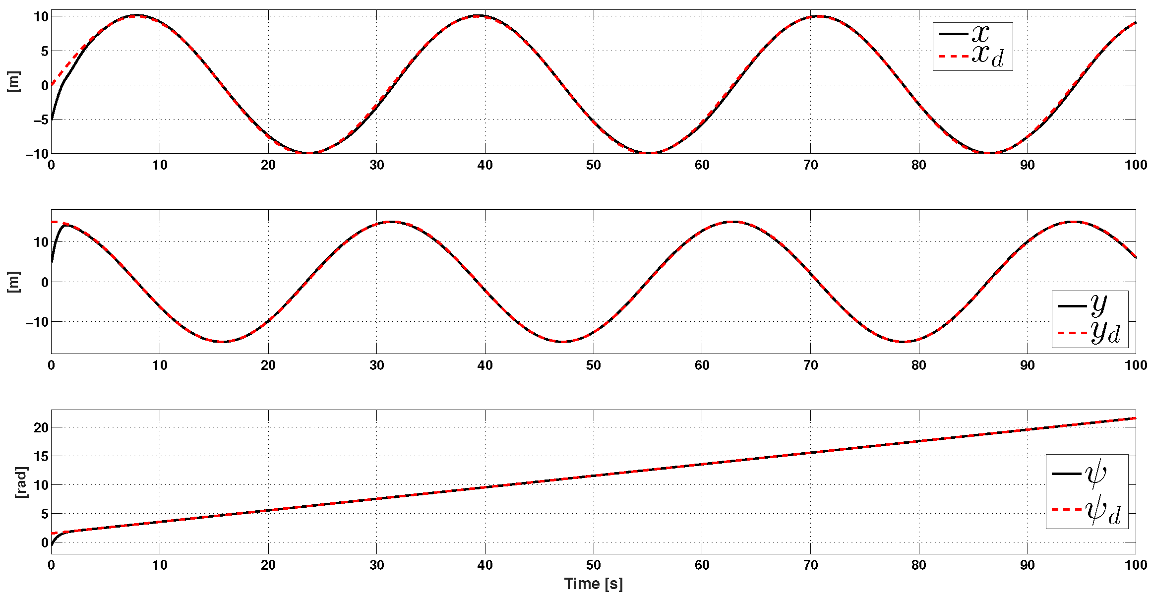
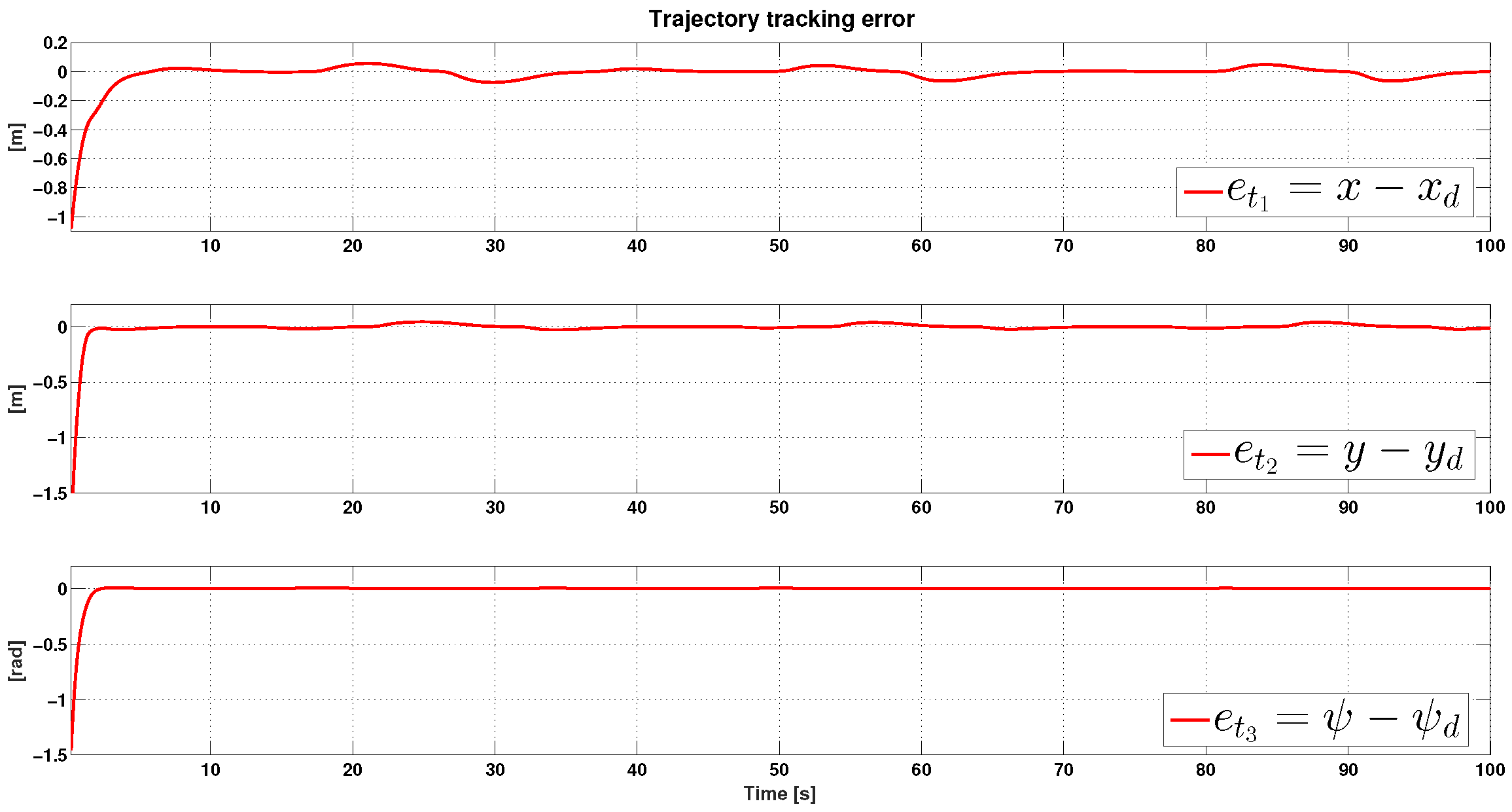
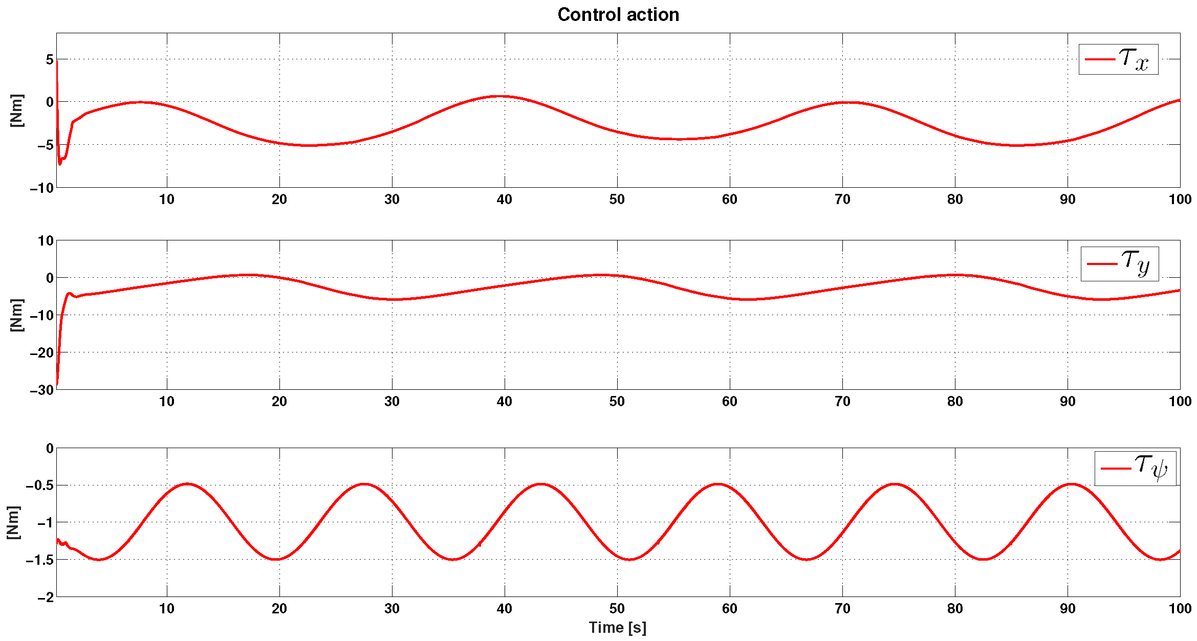
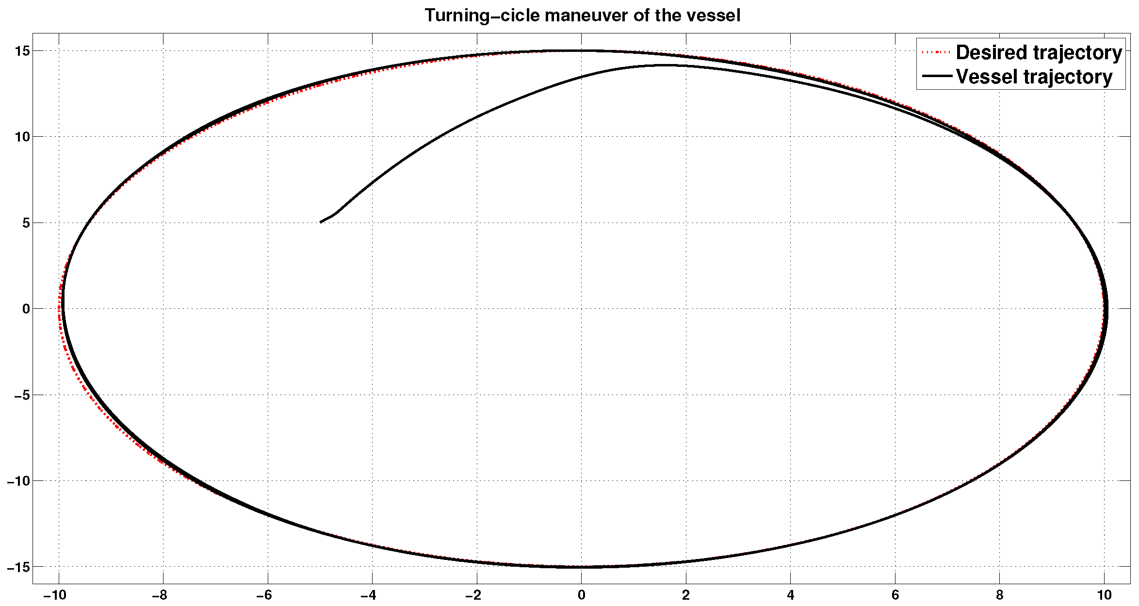
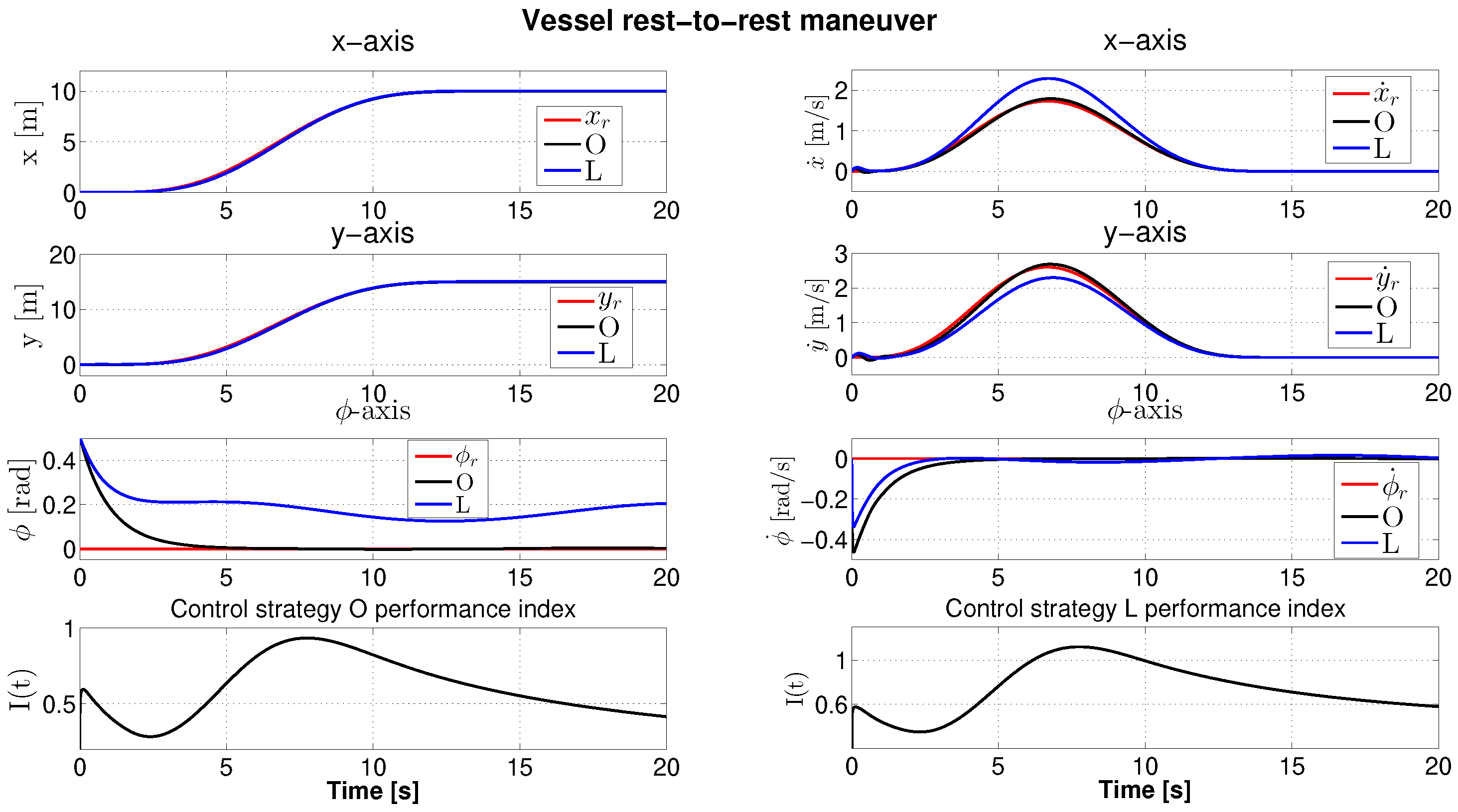
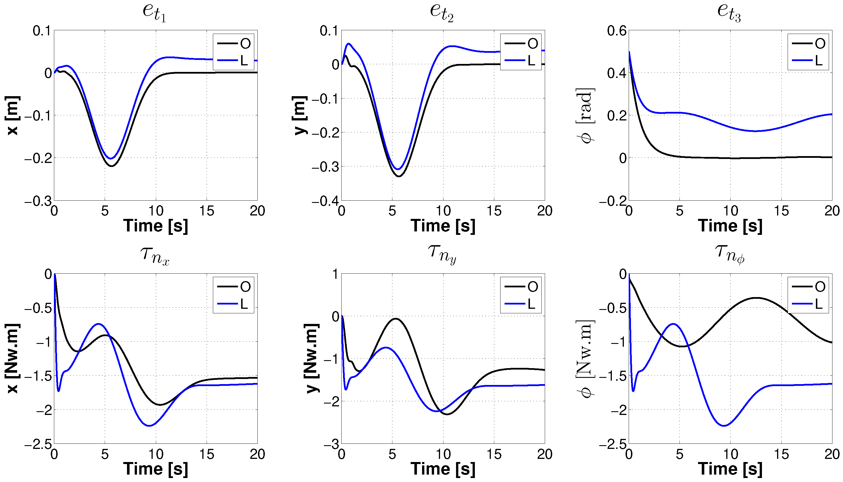
4. Numerical Simulations

To test the effectiveness of our control strategy, we designed two numerical experiments to assess that it performs well in terms of quick convergence of the tracking errors to a small neighborhood of zero, has smooth transient responses and low control effort, as well as tested its robustness, even when the vessel parameters and the external perturbation are entirely unknown. To this end, we use the parameter of an actual vessel (see [14]). For both experiments, we use the following setup; that is, the inertia matrix given by

$$M=\left[\begin{array}{ccc}1.1274& 0& 0\\ 0& 1.8902& -0.0744\\ 0& -0.0744& 0.1274\end{array}\right],$$

while the damping matrix is fixed as

$$D=\left[\begin{array}{ccc}0.0358& 0& 0\\ 0& 0.1183& -0.0124\\ 0& -0.0124& 0.0308\end{array}\right],$$

and the vessel is perturbed by the signal

$$\delta =\left[\begin{array}{c}1+0.2sin\left(0.1t\right)+cos\psi \\ 2+0.25cos\left(0.2t\right)+sin\psi \\ 2+sin\left(0.1t\right)\ast cos\left(0.2t\right)+2sin\psi \end{array}\right].$$

To accomplish the sliding mode and avoid the chattering phenomena, we use the following approximation:

$$\mathrm{sign}\left(s\right)={\displaystyle \frac{s}{\left|s\right|+0.001}}.$$

(30)

The first experiment: The task consists of a turning ellipse maneuver of the vessel, whose parameters are unknown. This experiment allows us to verify that the fast error converges to a small neighborhood of zero, as well as to verify the control law robustness against unmodeled, unmatched perturbations. In these simulations, the proposed ellipse trajectory is defined in the Earth’s fixed coordinate frame and centered around the origin. Then, we defined the reference trajectory as

$${\eta }_d\left(t\right)=\left[\begin{array}{c}{x}_d=10sin\left(0.2t\right)\\ y_d=15cos\left(0.2t\right)\\ {\psi }_d=0.2t+\pi /2\end{array}\right].$$

We set the initial conditions as $\eta \left(0\right)=(5 m,-7.5 m,-0.5 rad)$ and $v\left(0\right)=(0,0,0)$, and fixed the control gains as

$$\begin{array}{cccccc}{k}_p=10;& k_I=-25;& \kappa =0.1;& \rho =1;& \mathsf{\Lambda }=diag(1,2,2);& {\beta }_i=0.01\end{array}$$

for $i\in \{0,1,2\}$. The outcome of this experiment can be seen in Figure 2, Figure 3, Figure 4 and Figure 5. In Figure 2, we show actual and desired positions $(\eta ,{\eta }_d)$. This figure shows that the desired position coordinates $(x,y,\psi )$ are reached at close to 5, 2, and 1 s, respectively. At the same time, the corresponding tracking errors $(e_{t_1},e_{t_2},e_{t_3})$ are shown in Figure 3, where we can see that these errors are confined in a small neighborhood of zero. We present the input torques in Figure 4. This figure shows smooth behavior, a low control effort, and, due to the approximation in (30), the absence of the undesired chattering phenomena as a result. Finally, in Figure 5, we show the $x-y$ phase portrait plotter to give a concise image of the vessel maneuver. Additionally, in this figure, we can see that our control strategy effectively accomplishes the control task. We underscore that, to avoid the chattering phenomena, we filter the control effort by the first order low pass filter $G\left(s\right)={\displaystyle \frac{1}{s+1}}$. It is worth mentioning that the filtered controllers have the form of the reference signals with their respective perturbations. That is, these controllers counteract the effect of the undesirable perturbation. In addition, we can see that all signals reach the reference in a very small vicinity in a very short time.

The second experiment: 

In this control task, we accomplished a vessel rest-to-rest maneuver for the x and y axes within the finite time interval $[t_i, t_f]$ following a smooth interpolation polynomial. We specified the desired trajectory, ${\eta }_r\left(t\right)$, using the Bézier polynomial presented in [37], referred to here as $\mathsf{\Phi }(t,t_i, t_f)$, and satisfying the following conditions:

$$\begin{array}{ccc}\mathsf{\Phi }(t_i, t_i, t_f)=0& ,& \mathsf{\Phi }(t_f, t_i, t_f)=1\end{array},$$

where a finite number of the time derivatives of this interpolating polynomial were set to zero at the instants when the maneuver started and ended, which were at $t_i$ and $t_f$, respectively. In our case, we selected the desired trajectory as

$${\eta }_r\left(t\right)=\mathsf{\Phi }(t, t_i, t_f){\eta }_f,$$

where $\eta \left(0\right)=(0.1 \mathrm{m}, 0.1 \mathrm{m}, 0.5 \mathrm{rad})$ is the initial position, ${\eta }_f=(10 \mathrm{m}, 15 \mathrm{m}, 0 \mathrm{rad})$ is the final rest position, $t_i=0$ s is the initial time, and $t_f=15$ s is the time when the vessel reaches the final rest position. We used the same setup as before. Additionally, in this simulation, we assessed the performance of our control strategy (O) by comparing it against the performance of the following linearizing control (L) law:

$${\tau }_n=-k_{p}s+F\stackrel{.}{\eta }+C(\eta ,\stackrel{.}{\eta })\left(\stackrel{.}{\eta }-s\right)+J\left({\stackrel{..}{\eta }}_r+\mathsf{\Lambda }{\stackrel{.}{e}}_T+\stackrel{.}{\eta }\right),$$

(31)

where $k_p=10$ to make a fair comparison. To synthesize the control law L in (31), we needed to know the vessel’s physical parameters, matrices D and M, contrarily to our control law O, which can be seen as a black box with certainly known structure, since we based it on the MFCA. We show the obtained results in Figure 6 and Figure 7. The graphs in Figure 6 allow us to see that both strategies, O and L, effectively track the Bézier spline when carrying out the rest-to-rest maneuver in the x and y axes, with their corresponding velocities. In addition, this figure shows that the strategies track the vessel’s angular position and velocity close to zero. From these graphs, we can see that our strategy O outperforms strategy L. In the same figure, we can see the performance index of both strategies, defined as

$$I\left(t\right)={\displaystyle \frac{1}{t}}{\int }_0^t\sqrt{{∥e_T∥}^2+{∥{\stackrel{.}{e}}_T∥}^2}d\tau ,$$

which confirms that O performs better than L; that is, $I_O\to 0.45$ and $I_L=0.59$.

From the same simulation, we show in Figure 7 the tracking errors and the control actions of the closed loops of the O and L control strategies. Please note that to avoid the chattering phenomena and be able to make a comparison, we filter the control effort of our control strategy O using the first order low pass filter $G\left(s\right)={\displaystyle \frac{1}{s+1}}$. From the graphs in this figure, we can see that, when reaching the steady state, our control strategy performs better than the linearizing controller L, particularly in the performance of angle $\psi$. Related to the controllers’ response, we can see that they have similar behaviors, except the controller that acts over the vessel angle, due to the bias term ${\delta }_{\varphi }$ included in perturbation $\delta$.

5. Conclusions

We proposed a solution for the trajectory tracking problem of a fully actuated vessel with unknown parameters and perturbed by unknown, slowly varying external dynamics (wind, waves, and ocean currents). To design the controller, we assumed that the vessel moves at low speed and low frequency, its physical parameters are unknown, and its state is measurable. We used a nonlinear PID controller plus an adaptive sliding mode to solve the problem mentioned above as a model-free control problem. The obtained strategy ensures tracking error converges toward a small vicinity at the origin. This vicinity can be as small as desired. To carry out the stability analysis, we use the Lyapunov theory. To test the effectiveness of our controller, we designed and ran numerical experiments. The obtained results confirm that our approach accomplished the tracking trajectory control problem. Finally, we numerically compare our control solution against the classical linearizing approach. The outcome of this comparison showed that our controller performs better than the linearizing one. The proposed control law can be improved in future work if the trajectory tracking error converges to zero through a novel slide mode formulation and the design of the control tasks to assess the corresponding effectiveness.

References

1. Fossen, T.I. Guidance and Control of Ocean Vehicles. Ph.D. Thesis, University of Trondheim, Trondheim, Norway, 1999. [Google Scholar]
2. Yuh, J. Design and control of autonomous underwater robots: A survey. Auton. Robot. 2000, 8, 7–24. [Google Scholar] [CrossRef]
3. Morales, R.; Sira-Ramírez, H.; Somolinos, J. Linear active disturbance rejection control of the hovercraft vessel model. Ocean Eng. 2015, 96, 100–108. [Google Scholar] [CrossRef]
4. Fantoni, I.; Lozano, R.; Mazenc, F.; Pettersen, K. Stabilization of a nonlinear underactuated hovercraft. In Proceedings of the 38th IEEE Conference on Decision and Control (Cat. No. 99CH36304), Phoenix, AZ, USA, 7–10 December 1999; Volume 3, pp. 2533–2538. [Google Scholar]
5. Soro, D.; Lozano, R. Stabilization of an underactuated ship using a linear time-varying control. In Proceedings of the 41st IEEE Conference on Decision and Control, Las Vegas, NV, USA, 10–13 December 2002; Volume 2, pp. 1693–1698. [Google Scholar]
6. Sira-Ramírez, H. Dynamic second-order sliding mode control of the hovercraft vessel. IEEE Trans. Control Syst. Technol. 2002, 10, 860–865. [Google Scholar] [CrossRef]
7. Loria, A.; Fossen, T.I.; Panteley, E. A separation principle for dynamic positioning of ships: Theoretical and experimental results. IEEE Trans. Control Syst. Technol. 2000, 8, 332–343. [Google Scholar] [CrossRef]
8. Fang, Y.; Zergeroglu, E.; De Queiroz, M.; Dawson, D.M. Global output feedback control of dynamically positioned surface vessels: An adaptive control approach. Mechatronics 2004, 14, 341–356. [Google Scholar] [CrossRef]
9. Tee, K.P.; Ge, S.S. Control of fully actuated ocean surface vessels using a class of feedforward approximators. IEEE Trans. Control Syst. Technol. 2006, 14, 750–756. [Google Scholar] [CrossRef]
10. Skjetne, R.; Fossen, T.I.; Kokotović, P.V. Adaptive maneuvering, with experiments, for a model ship in a marine control laboratory. Automatica 2005, 41, 289–298. [Google Scholar] [CrossRef]
11. Chen, M.; Ge, S.S.; How, B.V.E.; Choo, Y.S. Robust adaptive position mooring control for marine vessels. IEEE Trans. Control Syst. Technol. 2012, 21, 395–409. [Google Scholar] [CrossRef]
12. Do, K.D. Global robust and adaptive output feedback dynamic positioning of surface ships. J. Mar. Sci. Appl. 2011, 10, 325–332. [Google Scholar] [CrossRef]
13. Qin, H.; Li, C.; Sun, Y.; Deng, Z.; Liu, Y. Trajectory tracking control of unmanned surface vessels with input saturation and full-state constraints. Int. J. Adv. Robot. Syst. 2018, 15, 1729881418808113. [Google Scholar] [CrossRef]
14. Moreno-Valenzuela, J.; Acho-Zuppa, L. Dynamic positioning control of ships via relay observer design. Asian J. Control 2004, 6, 398–406. [Google Scholar] [CrossRef]
15. Qiu, B.; Wang, G.; Fan, Y.; Mu, D.; Sun, X. Robust adaptive trajectory linearization control for tracking control of surface vessels with modeling uncertainties under input saturation. IEEE Access 2018, 7, 5057–5070. [Google Scholar] [CrossRef]
16. Qin, H.; Li, C.; Sun, Y.; Wang, N. Adaptive trajectory tracking algorithm of unmanned surface vessel based on anti-windup compensator with full-state constraints. Ocean Eng. 2020, 200, 106906. [Google Scholar] [CrossRef]
17. Reyes-Báez, R.; van der Schaft, A.; Jayawardhana, B.; Donaire, A.; Pérez, T. Tracking control of marine craft in the port-Hamiltonian framework: A virtual differential passivity approach. In Proceedings of the 2019 18th European Control Conference (ECC), Naples, Italy, 25–28 June 2019; pp. 1636–1641. [Google Scholar]
18. Khaled, N.; Chalhoub, N. A dynamic model and a robust controller for a fully-actuated marine surface vessel. J. Vib. Control 2011, 17, 801–812. [Google Scholar] [CrossRef]
19. Yu, X.N.; Hao, L.Y.; Wang, X.L. Fault tolerant control for an unmanned surface vessel based on integral sliding mode state feedback control. Int. J. Control. Autom. Syst. 2022, 20, 2514–2522. [Google Scholar] [CrossRef]
20. Yao, Q. Fixed-time trajectory tracking control for unmanned surface vessels in the presence of model uncertainties and external disturbances. Int. J. Control 2022, 95, 1133–1143. [Google Scholar] [CrossRef]
21. Wright, R.G. Intelligent autonomous ship navigation using multi-sensor modalities. TransNav Int. J. Mar. Navig. Saf. Sea Transp. 2019, 13, 503–510. [Google Scholar] [CrossRef]
22. He, S.; Dai, S.L.; Luo, F. Asymptotic trajectory tracking control with guaranteed transient behavior for MSV with uncertain dynamics and external disturbances. IEEE Trans. Ind. Electron. 2018, 66, 3712–3720. [Google Scholar] [CrossRef]
23. Shen, Z.; Bi, Y.; Wang, Y.; Guo, C. MLP neural network-based recursive sliding mode dynamic surface control for trajectory tracking of fully actuated surface vessel subject to unknown dynamics and input saturation. Neurocomputing 2020, 377, 103–112. [Google Scholar] [CrossRef]
24. From, P.J.; Schjølberg, I.; Gravdahl, J.T.; Pettersen, K.Y.; Fossen, T.I. On the boundedness and skew-symmetric properties of the inertia and coriolis matrices for vehicle-manipulator systems. IFAC Proc. Vol. 2010, 43, 193–198. [Google Scholar] [CrossRef]
25. Ortega, R.; Spong, M.W. Adaptive motion control of rigid robots: A tutorial. Automatica 1989, 25, 877–888. [Google Scholar] [CrossRef]
26. Kelly, R.; Santibáñez, V.; Loría, A. Control of Robot Manipulators in Joint Space; Springer: Berlin/Heidelberg, Germany, 2005; Volume 693. [Google Scholar]
27. Sira-Ramírez, H.; López-Uribe, C.; Velasco-Villa, M. Linear observer-based active disturbance rejection control of the omnidirectional mobile robot. Asian J. Control 2013, 15, 51–63. [Google Scholar] [CrossRef]
28. Sira-Ramírez, H.; Luviano-Juárez, A.; Ramírez-Neria, M.; Zurita-Bustamante, E.W. Active Disturbance Rejection Control of Dynamic Systems: A Flatness Based Approach; Butterworth-Heinemann: Oxford, UK, 2018. [Google Scholar]
29. Davila, J.; Fridman, L.; Poznyak, A. Observation and identification of mechanical systems via second order sliding modes. In Proceedings of the International Workshop on Variable Structure Systems, 2006. VSS’06, Alghero, Italy, 5–7 June 2006; pp. 232–237. [Google Scholar]
30. Ferreira, A.; Bejarano, F.J.; Fridman, L.M. Robust control with exact uncertainties compensation: With or without chattering? IEEE Trans. Control Syst. Technol. 2010, 19, 969–975. [Google Scholar] [CrossRef]
31. Ríos, H.; Rosales, A.; Ferreira, A.; Dávilay, A. Robust regulation for a 3-DOF helicopter via sliding-modes control and observation techniques. In Proceedings of the 2010 American Control Conference, Baltimore, MD, USA, 30 June–2 July 2010; pp. 4427–4432. [Google Scholar]
32. Küchler, S.; Pregizer, C.; Eberharter, J.K.; Schneider, K.; Sawodny, O. Real-time estimation of a ship’s attitude. In Proceedings of the 2011 American Control Conference, San Francisco, CA, USA, 29 June–1 July 2011; pp. 2411–2416. [Google Scholar]
33. Rogne, R.H.; Bryne, T.H.; Fossen, T.I.; Johansen, T.A. MEMS-based inertial navigation on dynamically positioned ships: Dead reckoning. IFAC-PapersOnLine 2016, 49, 139–146. [Google Scholar] [CrossRef]
34. Roy, S.; Baldi, S.; Fridman, L.M. On adaptive sliding mode control without a priori bounded uncertainty. Automatica 2020, 111, 108650. [Google Scholar] [CrossRef]
35. Parra-Vega, V.; Arimoto, S.; Liu, Y.H.; Hirzinger, G.; Akella, P. Dynamic sliding PID control for tracking of robot manipulators: Theory and experiments. IEEE Trans. Robot. Autom. 2003, 19, 967–976. [Google Scholar] [CrossRef]
36. Ye, H.; Gui, W.; Liu, G.P. Stabilization of complex cascade systems using boundedness information in finite time. Int. J. Robust Nonlinear Control. IFAC-Affil. J. 2009, 19, 1150–1167. [Google Scholar] [CrossRef]
37. Sira-Ramirez, H.; Agrawal, S.K. Differentially Flat Systems; CRC Press: Boca Raton, FL, USA, 2004. [Google Scholar]
Figure 1. Vessel translational position relative to the Earth coordinate frame ( X E ,   Y E ).
Mathematics 12 02239 g001
Figure 2. The desired and actual positions ( η d , η ) .
Mathematics 12 02239 g002
Figure 3. Tracking position error ( e T ) .
Mathematics 12 02239 g003
Figure 4. Control action ( τ ) .
Mathematics 12 02239 g004
Figure 5. Turning ellipse maneuver of the vessel ( x y phase portrait).
Mathematics 12 02239 g005
Figure 6. A comparison of the closed-loop responses of O and L control strategies when tracking a Bézier spline trajectory to carry out a rest-to-rest maneuver for the x and y axes.
Mathematics 12 02239 g006
Figure 7. A comparison of errors and control actions of the closed-loop response of O and L control strategies when tracking a Bézier spline trajectory to carry out a rest-to-rest maneuver for the x and y axes.
Mathematics 12 02239 g007
Disclaimer/Publisher’s Note: The statements, opinions and data contained in all publications are solely those of the individual author(s) and contributor(s) and not of MDPI and/or the editor(s). MDPI and/or the editor(s) disclaim responsibility for any injury to people or property resulting from any ideas, methods, instructions or products referred to in the content.