Abstract
This study introduces the KdV–Caudrey–Dodd–Gibbon (KdV-CDGE) equation to describe long water waves, acoustic waves, plasma waves, and nonlinear optics. Employing a generalized new auxiliary equation scheme, we derive exact analytical wave solutions, revealing rational, exponential, trigonometric, and hyperbolic trigonometric structures. The model also produces periodic, dark, bright, singular, and other soliton wave profiles. We compute classical and translational symmetries to develop abelian algebra, and visualize our results using selected parameters.
Keywords:
mathematical model; visualization; Lie theory; abelian algebra; identification of essential parameters MSC:
76M60; 35-00; 70H33
1. Introduction
Nonlinear evolution equations (NLEEs), which people have been desperately pursuing for a range of advanced applications, particularly the exact solution problem, remain the focus of both mathematicians and physicists [1,2]. Accordingly, investigations of the wave patterns for NLEEs have adequate significance in looking through nonlinear normal occasions [3]. NLEEs have numerous applications, including plasma physical science, computational physical science, optical fibers, water wave mechanics, the control hypothesis, meteorology, the electromagnetic hypothesis, mechanics, biogenetics, and more. Because of their repetitive appearance in different applications in physical science, science, design, the control hypothesis, money, and elements, the wave patterns to NLPDEs have drawn the consideration of many investigations. The analytical results of NLPDEs assume a significant part in the investigation of nonlinear actual peculiarities [4].
It is essential to recall that analytical solutions to nonlinear PDEs (partial differential equations) are effective tools for describing measurable and unmeasurable features existing in nonlinear phenomena across different scientific fields. These include plasma physics, solid-state physics, optical fibers, and solitary wave theory, among many others. There are various methods to find the analytical solution of NLPDEs, such as the exponential-function technique [5], the HAM [6], the Hirota approach [7,8], the F-expansion approach [9], the Exp-function technique [10], the sine-Gordon approach [11], the modified Kudryashov technique [12], the first integral scheme [13], the power series [14], the unified scheme [15,16], the multi-symplectic RK approach [17], the generalized unified approach [18,19], the khater approach [20], and some other approaches [21,22,23,24,25,26,27,28,29,30,31].
The Lie symmetry method, which is being highlighted by experts in this field, is a fundamental method that can be used to discover exact solutions of NLPDEs. The success of the Newton–Raphson method is mainly attributed to its simplicity, concision, and effectiveness; this method is a landmark in solving nonlinear differential equations. It is necessary to emphasize that the Lie point symmetry method refers to one of the most powerful and efficient sets of tools to classify the group invariant solutions of differential equations [32,33,34,35]. It provides a lot of help in generating analytical solutions to nonlinear differential equations utilizing similarity variables, which helps you to reduce complex partial differential equations into ordinary differential equations to solve. In addition, optimality is an essential second aspect of Lie groups theory, where both partial differential equations are converted to either linear or nonlinear ordinary differential equations.
In this study, we tackle a nonlinear KdV–Caudrey–Dodd–Gibbon Equation [36,37] of the following form:
The KdV-CDG equation plays an important role in laser optics, plasma physics, other nonlinear sciences, and ocean dynamics [38,39]. In this research, the used boundary conditions are and , and and are arbitrary positive quantities. When in Equation (1), it turns into the Korteweg–de Vries (KdV) Equation [40]. When , it turns into the Caudrey–Dodd–Gibbon (CDG) Equation [41]. From the literature, some work has been carried out on this model. The adequate soliton solutions of Equation (1) were computed in [36]. In [37,42], soliton solutions of Equation (1) were computed with the extended hyperbolic function method.
GNAEM is used to construct the new wave patterns for the KdV-CDG equation. This method was effectively applied to our proposed equation, yielding more generalized and intriguing results that are quite valuable in nonlinear research, particularly applied mathematics. GNAEM is a more powerful tool than other tools present in the literature that are used for the construction of wave solutions. GNAEM gives us interesting wave solutions in the form of trigonometric and hyperbolic trigonometric function forms.
This research follows this structure: In Section 2, GNAEM and the multiplier effect will be discussed. Section 3 represents a Lie theory application to Equation (1). Section 4 presents the generalized system, a scheme for the reduction of similarity, and an application method. Section 5 contains a graphical solution behavior. Lastly, Section 6 reveals the research results.
2. Preliminaries
The Idea of the Proposed Method
In this portion, the general pattern of GNAEM is represented. Consider the general form of PDE [43],
where is a dependent variable.
Let us assume the following:
where is arbitrary constant. Taking the following transformation, Equation (3) converts Equation (2) to an ODE:
Suppose Equation (4) has solutions as follows:
where and are constants. We combine the best order nonlinear and linear terms in the balancing approach to derive the value of N using Equation (4):
The following results of Equation (6) hold:
- Type 1: When ,
- Type 2: When , ,
- Type 3: When , ,
- Type 4: When , ,
- Type 5: When , ,
- Type 6: When , ,
- Type 7: When ,
- Type 8: When , ,
- Type 9: When ,
3. Symmetry Analysis of Equation (1)
The Lie method is used to investigate the stated Equation (1). Assume the one-parameter Lie group of infinitesimal transformations [44,45,46,47]:
where is a group parameter. The corresponding Lie algebra of infnitesimal symmetries is generated utilizing vector fields:
Equation (23) produces a symmetry of Equation (1), and passes the Lie group specifications:
where
We have
where can be written as follows:
By applying the Lie symmetry invariance condition to Equation (1), we have an over-determined system of PDEs; then, solving this system, we have the following infinitesimals:
We obtain the following two-dimensional Lie algebra:
We observe that
4. Traveling Waves of Equation (1) by Abelian Algebra
According to Equation (27), the vector field develops an abelian algebra. We can present the most effective system for (23) as follows:
We have the following similarity variables:
using Equations (1) and (29), and we obtain the following ODE:
To find soliton solutions, we integrate Equation (30) while keeping the integration constant to have the value zero:
Balancing with , we obtain . Therefore, the solution according to Equation (1) can be formulated as
Inserting Equation (32) into Equation (31) and letting the coefficient of , approach zero results in the following:
Using Equation (33) and the solution sets defined in Section 2, Equation (1) yields the following descriptions for its solutions:
- For Family 1: When ,
- For Family 2: When , ,
- For Family 3: When , ,
- For Family 4: When , ,
- For Family 5: When , ,
- For Family 6: When , ,
- For Family 7: When ,
- For Family 8: When and
- For Family 9: When ,
- For Family 10: When , ,
5. Graphical Representations
The section for graphical representation shows how our results would be useful for emphasizing the relevance of a nonlinear wave equation. To achieve this, we exemplify the graphical representation of the solutions by assigning reasonable values to the parameters. It could be used to model the behavior of shallow water waves since the solutions derived are obtained. These models can be applied for forecasting the patterns of waves and their interactions, which can be essential for coast constructions, tsunami warnings, and marine transportation. These derived solutions can be used back in plasma physics for the description of the wave behavior in plasma like in fusion reactors or in space plasmas, which have importance in energy and space science.
- Figure 1 demonstrates the 3D and 2D versions of for , , , , , and .
 Figure 1. A 3D and 2D graphical representation of .
 - The plotted curves of can be seen for , , , , , and . Their corresponding values are shown in Figure 2.
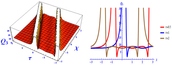 Figure 2. A 3D and 2D graphical representation of
 - The graphics of for , , , , and are shown in Figure 3. It shows the effect of the velocity of the soliton.
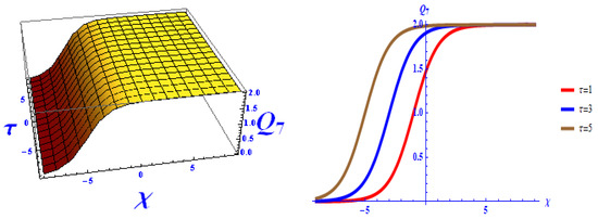 Figure 3. A 3D and 2D graphical representation of with positive velocity of the isolated states.
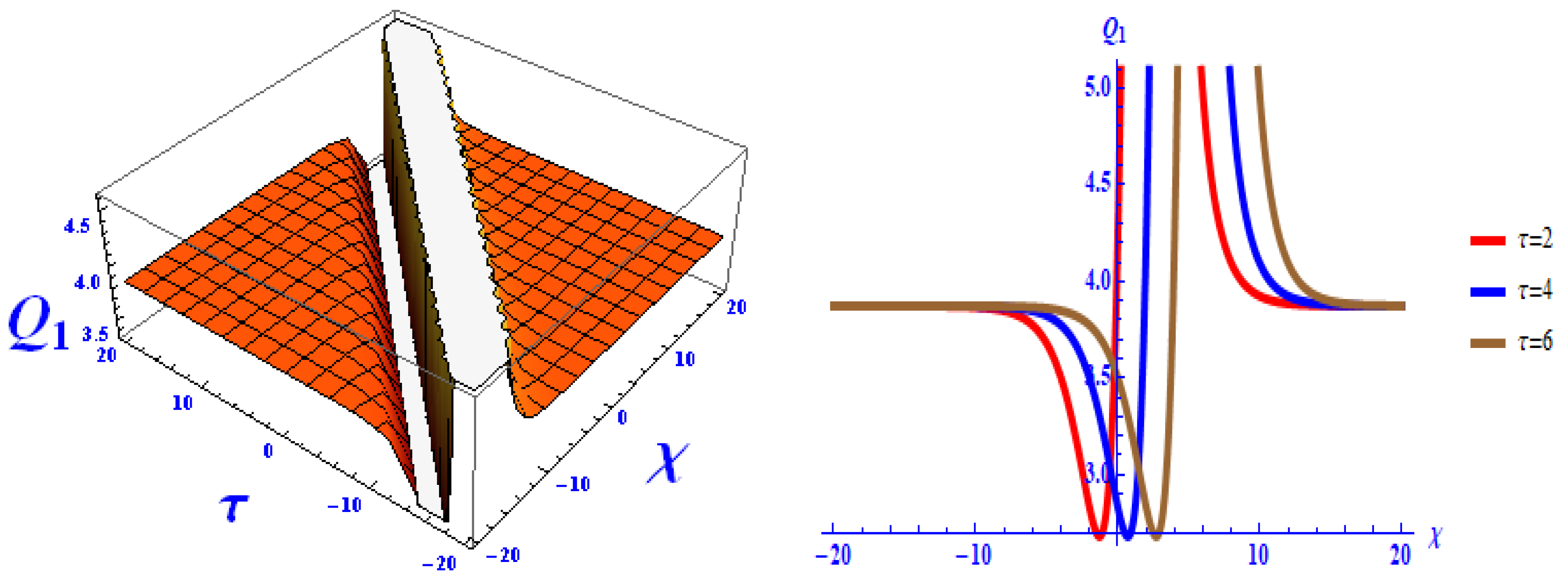
 - Furthermore, Figure 4 shows the 3D and 2D graph of for , , , , , and .
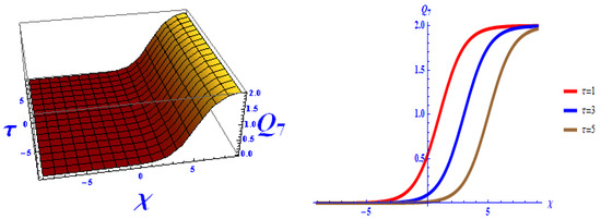 Figure 4. A 3D and 2D graphical representation of with negative velocity of the isolated states.
6. Conclusions
The present work presents a thorough examination of the KdV-CDG equation, emphasizing its numerous applications in nonlinear sciences. Through the application of the Lie group method, we successfully modeled and analyzed the equation, transforming nonlinear PDEs into manageable ODEs using similarity reduction. The implementation of GNAEM demonstrated its effectiveness in generating various wave patterns, underscoring its utility in solving nonlinear PDEs. Our graphical analysis clarified the physical consequences of our findings. By combining these results, we obtained a better understanding of the dynamics of gravity–capillary waves, shallow water waves, and magneto–sound wave interactions in plasma. Most importantly, our discovery of novel results presents new avenues for future research, marking a significant advancement in the field.
Author Contributions
Both authors (H.A. and A.J.) have contributed equally to this work. All authors have read and agreed to the published version of the manuscript.
Funding
The authors gratefully acknowledge the funding of the Deanship of Graduate Studies and Scientific Research, Jazan University, Saudi Arabia, through Project Number: GSSRD-24.
Data Availability Statement
Data sharing does not apply to this article as no datasets were generated or analyzed during the current study.
Conflicts of Interest
The authors declare no conflict of interest.
References
- Yang, Y.; Qi, J.M.; Tang, X.H.; Gu, Y.Y. Further Results about traveling wave exact solutions of the (2+1)-dimensional modified KdV equation. Adv. Math. Phys. 2019, 2019, 3053275. [Google Scholar] [CrossRef]
- Ilie, M.; Biazar, J.; Ayati, Z. The first integral method for solving some conformable fractional differential equations. Opt. Quantum Electron. 2018, 50, 55. [Google Scholar] [CrossRef]
- Akbar, M.A.; Ali, N.H.M.; Islam, M.T. Multiple closed-form solutions to some fractional order nonlinear evolution equations in physics and plasma physics. AIMS Math. 2019, 4, 397–411. [Google Scholar] [CrossRef]
- Liu, W.; Zhang, Y.; Triki, H.; Mirzazadeh, M.; Ekici, M.; Zhou, Q.; Biswas, A.; Belic, M. Interaction properties of solitonic in inhomogeneous optical fibers. Nonlinear Dyn. 2019, 95, 557–563. [Google Scholar] [CrossRef]
- Abdelrahman, M.; Zahran, E.H.M.; Khater, M.M.A. The exp(−ϕ(ξ))-expansion method and its application for solving nonlinear evolution equations. Int. J. Mod. Nonlinear Theory Appl. 2015, 4, 37–47. [Google Scholar] [CrossRef]
- Noor, N.F.M.; Haq, R.U.; Abbasbandy, S.; Hashim, I. Heat flux performance in a porous medium embedded Maxwell fluid flow over a vertically stretched plate due to heat absorption. J. Nonlinear Sci. Appl. 2016, 9, 2986–3001. [Google Scholar] [CrossRef]
- Ilhan, O.A.; Manafian, J.; Shahriari, M. Lump wave solutions and the interaction phenomenon for a variable-coefficient Kadomtsev-Petviashvili equation, Comput. Math. Appl. 2019, 78, 2429–2448. [Google Scholar]
- Manafian, J.; Ilhan, O.A.; Alizadeh, A. Periodic wave solutions and stability analysis for the KP-BBM equation with abundant novel interaction solutions. Phys. Scr. 2020, 95, 065203. [Google Scholar] [CrossRef]
- Akbar, M.A.; Ali, N.H.M. The improved F-expansion method with Riccati equation and its applications in mathematical physics. Cogent Math. 2017, 4, 1282577. [Google Scholar] [CrossRef]
- Zhang, S.; Li, J.; Zhang, L. A direct algorithm of exp-function method for non-linear evolution equations in fluids. Therm. Sci. 2016, 20, 881–884. [Google Scholar] [CrossRef]
- Baskonus, H.M.; Bulut, H.; Sulaiman, T.A. New complex hyperbolic structures to the Lonngren wave equation by using sine-Gordon expansion method. Appl. Math. Nonlinear Sci. 2019, 4, 129–138. [Google Scholar] [CrossRef]
- El-Sayed, M.F.; Moatimid, G.M.; Moussa, M.H.M.; El-Shiekh, R.M.; Khawlani, M.A. New exact solutions for coupled equal width wave equation and (2+1)-dimensional Nizhnik-Novikov-Veselov system using modified Kudryashov method. Int. J. Adv. Appl. Math. Mech. 2014, 2, 19–25. [Google Scholar]
- Akbar, M.A.; Ali, N.H.M.; Hussain, J. Optical soliton solutions to the (2+1)-dimensional Chaffee-Infante equation and the dimensionless form of the Zakharov equation. Adv. Differ. Equ. 2019, 2019, 446. [Google Scholar] [CrossRef]
- Jafari, M.; Mahdion, S.; Akgül, A.; Eldin, S.M. New conservation laws of the Boussinesq and generalized Kadomtsev—Petviashvili equations via homotopy operator. Results Phys. 2023, 1, 106369. [Google Scholar] [CrossRef]
- Osman, M.S.; Rezazadeh, H.; Eslami, M. Traveling wave solutions for (3+1) dimensional conformable fractional Zakharov-Kuznetsov equation with power law nonlinearity. Nonlinear Eng. 2019, 8, 559–567. [Google Scholar] [CrossRef]
- Osman, M.S. New analytical study of water waves described by coupled fractional variant Boussinesq equation in fluid dynamics. Pramana J. Phys. 2019, 93, 26. [Google Scholar] [CrossRef]
- Hu, W.P.; Deng, Z.C.; Han, S.M.; Fa, W. Multi-symplectic Runge-Kutta methods for Landau Ginzburg-Higgs equation. Appl. Math. Mech. 2009, 30, 1027–1034. [Google Scholar] [CrossRef]
- Osman, M.S. One-soliton shaping and inelastic collision between double solitons in the fifth-order variable-coefficient Sawada-Kotera equation. Nonlinear Dyn. 2019, 96, 1491–1496. [Google Scholar] [CrossRef]
- Javid, A.; Raza, N.; Osman, M.S. Multi-solitons of thermophoretic motion equation depicting the wrinkle propagation in substrate-supported graphene sheets. Commun. Theor. Phys. 2019, 71, 362–366. [Google Scholar] [CrossRef]
- Almusawa, H.; Jhangeer, A. Soliton solutions, Lie symmetry analysis and conservation laws of ionic waves traveling through microtubules in live cells. Results Phys. 2022, 43, 106028. [Google Scholar] [CrossRef]
- Jhangeer, A.; Hussain, A.; Junaid-U-Rehman, M.; Baleanu, D.; Riaz, M.B. Quasi-periodic, chaotic and traveling wave structures of modified Gardner equation. Chaos Solitons Fractals 2021, 143, 110578. [Google Scholar] [CrossRef]
- Hussain, A.; Jhangeer, A.; Abbas, N.; Khan, I. ESM Sherif Optical solitons of fractional complex Ginzburg–Landau equation with conformable, beta, and M-truncated derivatives: A comparative study. Adv. Differ. Equ. 2020, 1, 1–19. [Google Scholar]
- Jhangeer, A. Beenish, Study of magnetic fields using dynamical patterns and sensitivity analysis. Chaos Solitons Fractals 2024, 182, 114827. [Google Scholar] [CrossRef]
- Almusawa, H.; Alam, N.; Fayz-Al-Asad, M.; Osman, M.S. New soliton configurations for two different models related to the nonlinear Schrödinger equation through a graded-index waveguide. Aip. Adv. 2021, 11, 065320. [Google Scholar] [CrossRef]
- Malik, S.; Almusawa, H.; Kumar, S.; Wazwaz, A.M.; Osman, M.S. A (2+1)-dimensional Kadomtsev-Petviashvili equation with competing dispersion effect: Painlevé analysis, dynamical behavior and invariant solutions. Results Phys. 2021, 23, 104043. [Google Scholar] [CrossRef]
- Kumar, S.; Almusawa, H.; Kumar, A. Some more closed-form invariant solutions and dynamical behavior of multiple solitons for the (2+1)-dimensional rdDym equation using the Lie symmetry approach. Results Phys. 2021, 24, 104201. [Google Scholar] [CrossRef]
- Kumar, S.; Almusawa, H.; Hamid, I.; Abdou, M.A. Abundant closed-form solutions and solitonic structures to an integrable fifth-order generalized nonlinear evolution equation in plasma physics. Results Phys. 2021, 26, 104453. [Google Scholar] [CrossRef]
- Raslan, K.R.; Ali, K.K.; Shallal, M.A. The modified extended tanh method with the Riccati equation for solving the space-time fractional EW and MEW equations. Chaos Solitons Fractals 2017, 103, 404–409. [Google Scholar] [CrossRef]
- Rezazadeh, H.; Osman, M.S.; Eslami, M.; Mirzazadeh, M.; Zhou, Q.; Badri, S.A.; Korkmaz, A. Hyperbolic rational solutions to a variety of conformable fractional Boussinesqlike equations. Nonlinear Eng. 2019, 8, 224–230. [Google Scholar] [CrossRef]
- Islam, R.; Khan, K.; Akbar, M.A.; Islam, M.E.; Ahmed, M.T. Traveling wave solutions of some nonlinear evolution equations. Alex. Eng. J. 2015, 54, 263–269. [Google Scholar]
- Ghanbari, B.; Osman, M.S.; Baleanu, D. Generalized exponential rational function method for extended Zakharov Kuznetsov equation with conformable derivative. Mod. Phys. Lett. A 2019, 34, 1950155. [Google Scholar] [CrossRef]
- Ansari, A.R.; Jhangeer, A.; Imran, M.; Beenish; Inc, M. A study of self-adjointness, Lie analysis, wave structures, and conservation laws of the completely generalized shallow water equation. Eur. Phys. J. Plus 2024, 139, 489. [Google Scholar] [CrossRef]
- Riaz, M.B.; Awrejcewicz, J.; Jhangeer, A.; Junaid-U-Rehman, M. A Variety of New Traveling Wave Packets and Conservation Laws to the Nonlinear Low-Pass Electrical Transmission Lines via Lie Analysis. Fractal Fract. 2021, 5, 170. [Google Scholar] [CrossRef]
- Jhangeer, A.; Hussain, A.; Junaid-U-Rehman, M.; Khan, I.; Baleanu, D.; Nisar, K.S. Lie analysis, conservation laws and traveling wave structures of nonlinear Bogoyavlenskii–Kadomtsev–Petviashvili equation. Results Phys. 2020, 19, 103492. [Google Scholar] [CrossRef]
- Kurkcu, H.; Riaz, M.B.; Imran, M.; Jhangeer, A. Lie analysis and nonlinear propagating waves of the (3+1)-dimensional generalized Boiti–Leon–Manna–Pempinelli equation. Alex. Eng. J. 2023, 80, 475. [Google Scholar]
- Akbar, M.A.; Ali, N.H.M.; Tanjim, T. Adequate soliton solutions to the perturbed Boussinesq equation and the KdV-Caudrey-Dodd-Gibbon equation. J. King Saud Univ. Sci. 2020, 32, 2777–2785. [Google Scholar] [CrossRef]
- Asjad, M.I.; Ur Rehman, H.; Ishfaq, Z.; Awrejcewicz, J.; Akgül, A.; Riaz, M.B. On Soliton Solutions of Perturbed Boussinesq and KdV-Caudery-Dodd-Gibbon Equations. Coatings 2021, 11, 1429. [Google Scholar] [CrossRef]
- Tu, J.M.; Tian, S.F.; Xu, M.J.; Zhang, T.T. Quasi-periodic waves and solitary waves to a generalized KdV-Caudrey-Dodd-Gibbon equation from fluid dynamics. Taiwanese J. Math. 2016, 20, 823–848. [Google Scholar] [CrossRef]
- Dehghan, M.; Manafian, J.; Saadatmandi, A. Solving nonlinear fractional partial differential equations using the homotopy analysis method. Numer. Methods Partial. Diff. Equ. 2010, 26, 448–479. [Google Scholar] [CrossRef]
- Ma, W.X.; Yo, Y. Solving the Korteweg-de Vries equation by its bilinear form: Wronskian solutions. Trans. Am. Math. Soc. 2005, 57, 1753–1778. [Google Scholar] [CrossRef]
- Rogers, C.; Carillo, S. On reciprocal properties of the Caudrey-Dodd-Gibbon and Kaup-Kupershmidt hierarchies. Phys. Scr. 1987, 36, 865. [Google Scholar] [CrossRef]
- Biswas, A.; Ebadi, G.; Triki, H.; Yildirim, A.; Yousefzadeh, N. Topological soliton and other exact solutions to KdV–Caudrey–Dodd–Gibbon equation. Results Math. 2013, 63, 687–703. [Google Scholar] [CrossRef]
- Akbulut, A.; Kaplan, M. Auxiliary equation method for time-fractional differential equations with conformable derivative. Comput. Math. Appl. 2018, 75, 876–882. [Google Scholar] [CrossRef]
- Bluman, G.W.; Peter, J. Olver, Applications of Lie Groups to Differential Equations; Springer Science & Business Media: Berlin/Heidelberg, Germany, 1993. [Google Scholar]
- Bluman, G.W. Applications of Symmetry Methods to Partial Differential Equations; Springer: Berlin/Heidelberg, Germany, 2010. [Google Scholar]
- Kour, B.; Kumar, S. Space time fractional Drinfel’d-Sokolov-Wilson system with time-dependent variable coefficients: Symmetry analysis, power series solutions and conservation laws. Eur. Phys. J. Plus 2019, 134, 467. [Google Scholar] [CrossRef]
- Kudryashov, N.A.; Lavrova, S.F.; Nifontov, D.R. Bifurcations of Phase Portraits, Exact Solutions and Conservation Laws of the Generalized Gerdjikov–Ivanov Model. Mathematics 2023, 11, 4760. [Google Scholar] [CrossRef]


Disclaimer/Publisher’s Note: The statements, opinions and data contained in all publications are solely those of the individual author(s) and contributor(s) and not of MDPI and/or the editor(s). MDPI and/or the editor(s) disclaim responsibility for any injury to people or property resulting from any ideas, methods, instructions or products referred to in the content. |
© 2024 by the authors. Licensee MDPI, Basel, Switzerland. This article is an open access article distributed under the terms and conditions of the Creative Commons Attribution (CC BY) license (https://creativecommons.org/licenses/by/4.0/).