Stability Analysis, Modulation Instability, and Beta-Time Fractional Exact Soliton Solutions to the Van der Waals Equation

Abstract

The study consists of the distinct types of the exact soliton solutions to an important model called the beta-time fractional (1 + 1)-dimensional non-linear Van der Waals equation. This model is used to explain the motion of molecules and materials. The Van der Waals equation explains the phase separation phenomenon. Noncovalent Van der Waals or dispersion forces usually have an effect on the structure, dynamics, stability, and function of molecules and materials in different branches of science, including biology, chemistry, materials science, and physics. Solutions are obtained, including dark, dark-singular, periodic wave, singular wave, and many more exact wave solutions by using the modified extended tanh function method. Using the fractional derivatives makes different solutions different from the existing solutions. The gained results will be of high importance in the interaction of quantum-mechanical fluctuations, granular matters, and other applications of the Van der Waals equation. The solutions may be useful in distinct fields of science and civil engineering, as well as some basic physical ones like those studied in geophysics. The results are verified and represented by two-dimensional, three-dimensional, and contour graphs by using Mathematica software. The obtained results are newer than the existing results. Stability analysis is also performed to check the stability of the concerned model. Furthermore, modulation instability is studied to study the stationary solutions of the concerned model. The results will be helpful in future studies of the concerned system. In the end, we can say that the method used is straightforward and dynamic, and it will be a useful tool for debating tough issues in a wide range of fields.

1. Introduction

Mathematical modeling has much importance in applied sciences and engineering. Many models in many branches of science and engineering have been developed, including the new generalized Bogoyavlensky–Konopelchenko model [1], the Oskolkov model [2], nonlinear fractional partial differential equations [3], fourth-order parabolic partial differential equations [4], the longitudinal wave equation [5], the Biswas–Arshed model [6], the Kundu–Mukherjee–Naskar model [7], the Single-Joint Robot Arm model [8], and the Landau–Ginzburg–Higgs equation [9]. Only a few years ago, the use of fractional derivatives in mathematical modeling played a significant role [10]. With the help of these nonlinear evolution equations (NLEEs), nonlinear science is utilized to explain various nonlinear phenomena and complex interaction behaviors in fluid mechanics, bioinformatics, traffic flow, and financial systems [11,12,13,14,15]. Nonlinear fractional partial differential equations are a more prominent way to represent any naturally occurring phenomenon, including the multimodal learning paradigm [16], multimodal hybrid parallel networks [17], the neural architecture method [18], the accurate automated extraction of coseismic deformation [19], and improved BPNN method [20]. Various mathematical models are represented in the form of involving different fractional derivatives, such as the conformable nonlinear coupled Schrödinger model [21], the beta fractional modified Benjamin Bona Mahony model [22], the Truncated M-fractional Westervelt model [23], and many more.

There are distinct techniques to obtain the exact soliton solutions, for instance, the generalized double auxiliary equation technique [24], the new Extended Direct Algebraic scheme [25], the Ricatti equation mapping technique [26], Paul Painleve’s technique [27], the improved Fan sub-equation approach [28], the enhanced algebraic method [29], the exponential rational function technique [30], the multiple exp-function scheme [31], the Hirota bilinear approach [32], the Jacobi elliptic function technique [33], the generalized exponential rational function approach [34], the modified Sardar sub-equation scheme [35], the improved modified extended tanh function technique [36], and the new extended hyperbolic function method [37].

A neural network identifier was built to estimate the unknown system dynamics, and a critic neural network was constructed to solve the Hamiltonian-Jacobi-Bellman equation associated with the optimal control problem [38]. The closed-form solitary wave solutions for the Ginzburg-Landau equation were obtained [39]. Two efficient techniques were employed to explore these solutions for the Chaffee-Infante equation [40]. The method integrates logarithmic transformations and the symbolic structures were used to obtain several trigonometric, hyperbolic, and rational expressions to nonlinear Zakharov system [41]. A generalization of the regularized long-wave equation was considered, and the existences of smooth soliton, peakon, and periodic solutions were established via the complete discrimination system for polynomial method and the bifurcation method [42]. The linear structure of Sharma-Tasso-Olver-Burgers equation was presented and a general form of the multi-wave solution was obtained [43]. A new closed-form design of wideband infinite impulse response digital integrators using numerical integration rules that were constructed via trigonometric interpolation [44].

Some of the nonlinear models examined using the mentioned methods in literature are as follows: a fast nonsingleton fuzzy predictive [45], the fuzzy neural network [46], the fractional-order fuzzy control [47], optimal deep learning control [48] and optical deposition method [49]. A notable models in this context is the nonlinear equations which offers a more precise interpretation of complex nonlinear models such as multimodal engineering optimization problems [50], deep convolutional neural networks [51], finger photoplethys-mography [52], multi-objects detection [53], and robust niching chimp optimization [54]. The nonlinear models belong to a class of nonlinear dynamical systems that have specific applications and implications in various fields and can exhibit rich dynamics, including chimp optimization method [55], improved chimp optimization method [56], an innovative algorithm for multi-objective problems [57], vision-language learning technique [58], virtual multiple quasi method [59].

Many approaches have been suggested by researchers in this context. Some of the methods that have attracted attention recently are as follows: network traffic detection model [60], generalized matrix completion [61], a robust observer method [62] quasi-Z-source inverter method [63], and fuzzy logic system [64].

In this paper, we used a simple and useful scheme: the modified extended tanh function scheme. The concerned scheme has been used for different models. For instance, the modified extended tanh function method is used for the Lakshmanan–Porsezian–Daniel equation [65], the coupled Klein–Gordon–Zakharov model [66], the Bogoyavlenskii model [67], the generalized Bugures–Fisher model [68], the Sharma–Tasso–Olveer equation [69], the complex Ginzburg-Landau equation [70], the phi-four equation [71], and the Sasa–Satsuma equation [72].

The basic aim of this paper is to explore new kinds of exact soliton solutions to the (1 + 1)-dimensional nonlinear Van der Waals equation along the beta-time fractional derivative. Additionally, stability analysis and modulation instability analysis are used to verify the stability and validity of the obtained solutions.

This paper has different sections: the governing equation and its mathematical analysis are given in Section 2, the modified extended tanh function scheme and its application are explained in Section 3, the graphic representation is shown in Section 4, the physical interpretation is given in Section 5, the stability analysis is given in Section 6, the modulation instability is explained in Section 7, and the conclusion is given in Section 8.

1.1. $\beta$-Time Derivative and Its Characteristics

Definition 1.

Consider $u(t)$ is defined for all non-negative t. Therefore, the beta-time fractional derivative of the function u of order θ is shown as follows [73]

$$\begin{array}{c}\hfill D^{\theta }(u(t))={\displaystyle \frac{d^{\theta }u(t)}{d{t}^{\theta }}}=\underset{ϵ\to 0}{lim}{\displaystyle \frac{u(t+ϵ{(t+\frac{1}{\Gamma (\theta )})}^{1-\theta })-u(t)}{ϵ}},0<\theta \le 1.\end{array}$$

Some of the main characteristics are given in [73,74,75].

1.2. Characteristics

Suppose $v(t)$ and $u(t)$ are the $\theta$—time differentiable functions ∀ t$>0$ and $\theta \in (0,1]$. Then

$$\begin{array}{c}\hfill i.D^{\theta }(av(t)+bu(t))=a{D}^{\theta }(v(t))+b{D}^{\theta }(u(t)),\forall a,b\in R.\end{array}$$

$$\begin{array}{c}\hfill ii.D^{\theta }(v(t)u(t))=u(t)D^{\theta }(v(t))+v(t)D^{\theta }(u(t)).\end{array}$$

$$\begin{array}{c}\hfill iii.D^{\theta }({\displaystyle \frac{v(t)}{u(t)}})={\displaystyle \frac{u(t)D^{\theta }(v(t))-v(t)D^{\theta }(u(t))}{{(u(t))}^2}}.\end{array}$$

$$\begin{array}{c}\hfill iv.D^{\theta }(v(t))={(t+{\displaystyle \frac{1}{\Gamma (\theta )}})}^{1-\theta }{\displaystyle \frac{dv(t)}{d\theta }}.\end{array}$$

2. Model Representation and Mathematical Analysis

Consider a nonlinear (1 + 1)-dimensional Van der Waals equation given as [76]

$$u_{tt}+u_{xxxx}-\alpha u_{xxt}-{(u^3)}_{xx}-\beta u_{xx}=0,$$

(1)

where $u=u(x,t)$ is a wave profile depending on the spatial variable x and temporal variable t, while $\alpha$ and $\beta$ are the non-zero constants. $\alpha$ represents an effective viscosity, while $\beta$ denotes a bifurcation parameter. Equation (1) is linked with natural phenomena and industrial applications. This equation also plays an important role in geophysics, civil engineering, pharmaceuticals, etc. Different techniques are used for Equation (1) in the literature, including the extended $(G^{\prime }/G)$-expansion scheme [76], the generalized Kudryashov technique [77], the simplest equation scheme [78], the extended sinh-Gordon equation expansion technique [79], and many more.

Suppose the nonlinear (1 + 1)-dimensional Van der Waals equation in the beta-time fractional derivative is given as

$${\displaystyle \frac{{\partial }^{2\theta }u}{\partial t^{2\theta }}}+{\displaystyle \frac{{\partial }^{4\theta }u}{\partial x^{4\theta }}}-\alpha {\displaystyle \frac{{\partial }^{2\theta }}{\partial x^{2\theta }}}({\displaystyle \frac{{\partial }^{\theta }u}{\partial t^{\theta }}})-{\displaystyle \frac{{\partial }^{2\theta }}{\partial x^{2\theta }}}{u}^3-\beta {\displaystyle \frac{{\partial }^{2\theta }u}{\partial x^{2\theta }}}=0.$$

(2)

Assume a wave transformation is given as

$$u(x,t)=U(\zeta ),\zeta =(\mu {\displaystyle \frac{1}{\theta }}{(x+{\displaystyle \frac{1}{\Gamma (\theta )}})}^{\theta }-\omega {\displaystyle \frac{1}{\theta }}{(t+{\displaystyle \frac{1}{\Gamma (\theta )}})}^{\theta }),$$

(3)

where $U^{″}$ represents the profile function, which describes the shape of the wave, while $\mu$ and $\omega$ are the non-zero constants.

By using Equation (3) into Equation (2) and integrating twice with respect to $\zeta$, one gains

$$\left({\omega }^2-\beta {\mu }^2\right)U-{\mu }^2{U}^3+\alpha {\mu }^2\omega U^{\prime }+{\mu }^4{U}^{″}=0.$$

(4)

We obtain a value of m by applying the homogenous balance scheme to Equation (4) as follows:

By balancing the terms $U^{″}$ and $U^3$ we obtain

$$3m=m+2,\mathrm{so}m=1.$$

Next, we will explain the methods and find the exact wave solitons of Equation (4).

3. Description of METhF Technique

Here, some of the main steps of the method are given. Assuming a conformable fractional NLPDE:

$$\chi (v,v^2,\dots ,{\displaystyle \frac{{\partial }^{\alpha }v}{\partial t^{\alpha }}},{\displaystyle \frac{{\partial }^{2\alpha }v}{\partial t^{2\alpha }}},\dots ,{\displaystyle \frac{\partial v}{\partial x}},{\displaystyle \frac{{\partial }^{2}v}{\partial x^2}},\dots )=0,$$

(5)

where $v=v(x,t)$ shows a wave profile. Consider the following transformation

$$v(x,t)=V(\zeta ),\zeta =\mu (x-\nu {\displaystyle \frac{t^{\alpha }}{\alpha }}),$$

(6)

where $\nu$ denotes a soliton speed. Using Equation (6) in Equation (5), yields

$$\chi (V,V^2,\mu V^{\prime },\mu {\nu }^2{V}^{″},\dots )=0.$$

(7)

Consider the solution of Equation (7) is shown as

$$V(\zeta )=a_0+\sum _{j=1}^m{a}_j{\phi }^j(\zeta )+\sum _{j=1}^m{b}_j{\phi }^{-j}(\zeta ),$$

(8)

where $a_0,a_j,b_j,(j=1,2,3,\dots ,m)$ are undetermined.

$\phi (\zeta )$ fulfills the following:

$${\phi }^{\prime }(\zeta )=\delta +{\phi }^2(\zeta ),$$

(9)

where $\delta$ is a constant, and the solution of Equation (9) is shown in [80]:

If $\delta$ is negative, then we have

$$\phi (\zeta )=-\sqrt{-\delta }tanh(\sqrt{-\delta }\zeta ),$$

(10)

or

$$\phi (\zeta )=-\sqrt{-\delta }coth(\sqrt{-\delta }\zeta ).$$

(11)

If $\delta$ is zero, then we have

$$\phi (\zeta )={\displaystyle \frac{-1}{\zeta }}.$$

(12)

If $\delta$ is positive, then we get

$$\phi (\zeta )=\sqrt{\delta }tan(\sqrt{\delta }\zeta ),$$

(13)

or

$$\phi (\zeta )=-\sqrt{\delta }cot(\sqrt{\delta }\zeta ).$$

(14)

Put Equations (8) and (9) into Equation (7). Collecting the co-efficient of $\phi (\zeta )$ of every power and putting it to zero, one obtains sets of equations including $a_0,a_j,b_j(j=1,2,3,\dots ,m)$, and $\delta$. By manumitting the obtained equations, we obtain the results for Equation (5).

Application to the METhF Technique

For $m=1$, the Equation (8) reduces to

$$U(\zeta )=a_0+a_1\phi (\zeta )+b_1\phi {(\zeta )}^{-1},$$

(15)

Applying Equation (15) into Equation (4) along with Equation (9), one obtains a system containing $a_0$, $a_1$, $b_1$, $\omega$ and $\delta$. Solving the system yields the following sets.

Set 1:

$$\{a_0=\mp {\displaystyle \frac{\alpha \sqrt{\beta }}{\sqrt{18-4{\alpha }^2}}},a_1=0,b_1=\pm {\displaystyle \frac{\alpha \sqrt{2{\alpha }^2-9}\sqrt{\beta \delta }}{\sqrt{2}(2{\alpha }^2-9)}},\omega ={\displaystyle \frac{3\alpha \beta }{2(2{\alpha }^2-9)\sqrt{-\delta }}},\mu ={\displaystyle \frac{\alpha \sqrt{\beta }}{\sqrt{(8{\alpha }^2-36)\delta }}}\}.$$

(16)

Case 1: For $\delta <0$:

$$\begin{array}{c}u(x,t)=\mp {\displaystyle \frac{\alpha \sqrt{\beta }}{\sqrt{18-4{\alpha }^2}}}\pm {\displaystyle \frac{\alpha \sqrt{2{\alpha }^2-9}\sqrt{\beta \delta }}{\sqrt{2}(2{\alpha }^2-9)}}(-\sqrt{-\delta }tanh(\sqrt{-\delta }({\displaystyle \frac{\alpha \sqrt{\beta }}{\sqrt{(8{\alpha }^2-36)\delta }}}{\displaystyle \frac{1}{\theta }}{(x+{\displaystyle \frac{1}{\Gamma (\theta )}})}^{\theta }\hfill \\ \hfill -{\displaystyle \frac{3\alpha \beta }{2(2{\alpha }^2-9)\sqrt{-\delta }}}{\displaystyle \frac{1}{\theta }}{(t+{\displaystyle \frac{1}{\Gamma (\theta )}})}^{\theta }{)))}^{-1},\end{array}$$

(17)

or

$$\begin{array}{c}u(x,t)=\mp {\displaystyle \frac{\alpha \sqrt{\beta }}{\sqrt{18-4{\alpha }^2}}}\pm {\displaystyle \frac{\alpha \sqrt{2{\alpha }^2-9}\sqrt{\beta \delta }}{\sqrt{2}(2{\alpha }^2-9)}}(-\sqrt{-\delta }coth(\sqrt{-\delta }({\displaystyle \frac{\alpha \sqrt{\beta }}{\sqrt{(8{\alpha }^2-36)\delta }}}{\displaystyle \frac{1}{\theta }}{(x+{\displaystyle \frac{1}{\Gamma (\theta )}})}^{\theta }\hfill \\ \hfill -{\displaystyle \frac{3\alpha \beta }{2(2{\alpha }^2-9)\sqrt{-\delta }}}{\displaystyle \frac{1}{\theta }}{(t+{\displaystyle \frac{1}{\Gamma (\theta )}})}^{\theta }{)))}^{-1}.\end{array}$$

(18)

Case 3: For $\delta >0$:

$$\begin{array}{c}u(x,t)=\mp {\displaystyle \frac{\alpha \sqrt{\beta }}{\sqrt{18-4{\alpha }^2}}}\pm {\displaystyle \frac{\alpha \sqrt{2{\alpha }^2-9}\sqrt{\beta \delta }}{\sqrt{2}(2{\alpha }^2-9)}}(\sqrt{\delta }tan(\sqrt{\delta }({\displaystyle \frac{\alpha \sqrt{\beta }}{\sqrt{(8{\alpha }^2-36)\delta }}}{\displaystyle \frac{1}{\theta }}{(x+{\displaystyle \frac{1}{\Gamma (\theta )}})}^{\theta }\hfill \\ \hfill -{\displaystyle \frac{3\alpha \beta }{2(2{\alpha }^2-9)\sqrt{-\delta }}}{\displaystyle \frac{1}{\theta }}{(t+{\displaystyle \frac{1}{\Gamma (\theta )}})}^{\theta }{)))}^{-1},\end{array}$$

(19)

or

$$\begin{array}{c}u(x,t)=\mp {\displaystyle \frac{\alpha \sqrt{\beta }}{\sqrt{18-4{\alpha }^2}}}\pm {\displaystyle \frac{\alpha \sqrt{2{\alpha }^2-9}\sqrt{\beta \delta }}{\sqrt{2}(2{\alpha }^2-9)}}(-\sqrt{\delta }cot(\sqrt{\delta }({\displaystyle \frac{\alpha \sqrt{\beta }}{\sqrt{(8{\alpha }^2-36)\delta }}}{\displaystyle \frac{1}{\theta }}{(x+{\displaystyle \frac{1}{\Gamma (\theta )}})}^{\theta }\hfill \\ \hfill -{\displaystyle \frac{3\alpha \beta }{2(2{\alpha }^2-9)\sqrt{-\delta }}}{\displaystyle \frac{1}{\theta }}{(t+{\displaystyle \frac{1}{\Gamma (\theta )}})}^{\theta }{)))}^{-1}.\end{array}$$

(20)

Set 2:

$$\{a_0=\pm {\displaystyle \frac{\alpha \sqrt{\beta }}{\sqrt{18-4{\alpha }^2}}},a_1=\pm {\displaystyle \frac{\alpha \sqrt{2{\alpha }^2-9}\sqrt{\beta }}{(2{\alpha }^2-9)\sqrt{2\delta }}},b_1=0,\omega ={\displaystyle \frac{3\alpha \beta }{2(2{\alpha }^2-9)\sqrt{-\delta }}},\mu ={\displaystyle \frac{\alpha \sqrt{\beta }}{\sqrt{(8{\alpha }^2-36)\delta }}}\}.$$

(21)

Case 1: For $\delta <0$:

$$\begin{array}{c}u(x,t)=\pm {\displaystyle \frac{\alpha \sqrt{\beta }}{\sqrt{18-4{\alpha }^2}}}\pm {\displaystyle \frac{\alpha \sqrt{2{\alpha }^2-9}\sqrt{\beta }}{(2{\alpha }^2-9)\sqrt{2\delta }}}(-\sqrt{-\delta }tanh(\sqrt{-\delta }({\displaystyle \frac{\alpha \sqrt{\beta }}{\sqrt{(8{\alpha }^2-36)\delta }}}{\displaystyle \frac{1}{\theta }}{(x+{\displaystyle \frac{1}{\Gamma (\theta )}})}^{\theta }\hfill \\ \hfill -{\displaystyle \frac{3\alpha \beta }{2(2{\alpha }^2-9)\sqrt{-\delta }}}{\displaystyle \frac{1}{\theta }}{(t+{\displaystyle \frac{1}{\Gamma (\theta )}})}^{\theta }))),\end{array}$$

(22)

or

$$\begin{array}{c}u(x,t)=\pm {\displaystyle \frac{\alpha \sqrt{\beta }}{\sqrt{18-4{\alpha }^2}}}\pm {\displaystyle \frac{\alpha \sqrt{2{\alpha }^2-9}\sqrt{\beta }}{(2{\alpha }^2-9)\sqrt{2\delta }}}(-\sqrt{-\delta }coth(\sqrt{-\delta }({\displaystyle \frac{\alpha \sqrt{\beta }}{\sqrt{(8{\alpha }^2-36)\delta }}}{\displaystyle \frac{1}{\theta }}{(x+{\displaystyle \frac{1}{\Gamma (\theta )}})}^{\theta }\hfill \\ \hfill -{\displaystyle \frac{3\alpha \beta }{2(2{\alpha }^2-9)\sqrt{-\delta }}}{\displaystyle \frac{1}{\theta }}{(t+{\displaystyle \frac{1}{\Gamma (\theta )}})}^{\theta }))).\end{array}$$

(23)

Case 3: For $\delta >0$:

$$\begin{array}{c}u(x,t)=\pm {\displaystyle \frac{\alpha \sqrt{\beta }}{\sqrt{18-4{\alpha }^2}}}\pm {\displaystyle \frac{\alpha \sqrt{2{\alpha }^2-9}\sqrt{\beta }}{(2{\alpha }^2-9)\sqrt{2\delta }}}(\sqrt{\delta }tan(\sqrt{\delta }({\displaystyle \frac{\alpha \sqrt{\beta }}{\sqrt{(8{\alpha }^2-36)\delta }}}{\displaystyle \frac{1}{\theta }}{(x+{\displaystyle \frac{1}{\Gamma (\theta )}})}^{\theta }\hfill \\ \hfill -{\displaystyle \frac{3\alpha \beta }{2(2{\alpha }^2-9)\sqrt{-\delta }}}{\displaystyle \frac{1}{\theta }}{(t+{\displaystyle \frac{1}{\Gamma (\theta )}})}^{\theta }))),\end{array}$$

(24)

or

$$\begin{array}{c}u(x,t)=\pm {\displaystyle \frac{\alpha \sqrt{\beta }}{\sqrt{18-4{\alpha }^2}}}\pm {\displaystyle \frac{\alpha \sqrt{2{\alpha }^2-9}\sqrt{\beta }}{(2{\alpha }^2-9)\sqrt{2\delta }}}(-\sqrt{\delta }cot(\sqrt{\delta }({\displaystyle \frac{\alpha \sqrt{\beta }}{\sqrt{(8{\alpha }^2-36)\delta }}}{\displaystyle \frac{1}{\theta }}{(x+{\displaystyle \frac{1}{\Gamma (\theta )}})}^{\theta }\hfill \\ \hfill -{\displaystyle \frac{3\alpha \beta }{2(2{\alpha }^2-9)\sqrt{-\delta }}}{\displaystyle \frac{1}{\theta }}{(t+{\displaystyle \frac{1}{\Gamma (\theta )}})}^{\theta }))).\end{array}$$

(25)

Set 3:

$$\begin{array}{c}\{a_0=\pm {\displaystyle \frac{\alpha \sqrt{\beta }}{\sqrt{18-4{\alpha }^2}}},a_1=0,b_1=\pm {\displaystyle \frac{\alpha \sqrt{2{\alpha }^2-9}\sqrt{\beta \delta }}{\sqrt{2}(2{\alpha }^2-9)}},\omega =-{\displaystyle \frac{3\alpha \beta }{2(2{\alpha }^2-9)\sqrt{-\delta }}},\hfill \\ \hfill \mu ={\displaystyle \frac{\alpha \sqrt{\beta }}{\sqrt{(8{\alpha }^2-36)\delta }}}\}.\end{array}$$

(26)

Case 1: For $\delta <0$:

$$\begin{array}{c}u(x,t)=\pm {\displaystyle \frac{\alpha \sqrt{\beta }}{\sqrt{18-4{\alpha }^2}}}\pm {\displaystyle \frac{\alpha \sqrt{2{\alpha }^2-9}\sqrt{\beta \delta }}{\sqrt{2}(2{\alpha }^2-9)}}(-\sqrt{-\delta }tanh(\sqrt{-\delta }({\displaystyle \frac{\alpha \sqrt{\beta }}{\sqrt{(8{\alpha }^2-36)\delta }}}{\displaystyle \frac{1}{\theta }}{(x+{\displaystyle \frac{1}{\Gamma (\theta )}})}^{\theta }\hfill \\ \hfill +{\displaystyle \frac{3\alpha \beta }{2(2{\alpha }^2-9)\sqrt{-\delta }}}{\displaystyle \frac{1}{\theta }}{(t+{\displaystyle \frac{1}{\Gamma (\theta )}})}^{\theta }{)))}^{-1},\end{array}$$

(27)

or

$$\begin{array}{c}u(x,t)=\pm {\displaystyle \frac{\alpha \sqrt{\beta }}{\sqrt{18-4{\alpha }^2}}}\pm {\displaystyle \frac{\alpha \sqrt{2{\alpha }^2-9}\sqrt{\beta \delta }}{\sqrt{2}(2{\alpha }^2-9)}}(-\sqrt{-\delta }coth(\sqrt{-\delta }({\displaystyle \frac{\alpha \sqrt{\beta }}{\sqrt{(8{\alpha }^2-36)\delta }}}{\displaystyle \frac{1}{\theta }}{(x+{\displaystyle \frac{1}{\Gamma (\theta )}})}^{\theta }\hfill \\ \hfill +{\displaystyle \frac{3\alpha \beta }{2(2{\alpha }^2-9)\sqrt{-\delta }}}{\displaystyle \frac{1}{\theta }}{(t+{\displaystyle \frac{1}{\Gamma (\theta )}})}^{\theta }{)))}^{-1}.\end{array}$$

(28)

Case 3: For $\delta >0$:

$$\begin{array}{c}u(x,t)=\pm {\displaystyle \frac{\alpha \sqrt{\beta }}{\sqrt{18-4{\alpha }^2}}}\pm {\displaystyle \frac{\alpha \sqrt{2{\alpha }^2-9}\sqrt{\beta \delta }}{\sqrt{2}(2{\alpha }^2-9)}}(\sqrt{\delta }tan(\sqrt{\delta }({\displaystyle \frac{\alpha \sqrt{\beta }}{\sqrt{(8{\alpha }^2-36)\delta }}}{\displaystyle \frac{1}{\theta }}{(x+{\displaystyle \frac{1}{\Gamma (\theta )}})}^{\theta }\hfill \\ \hfill +{\displaystyle \frac{3\alpha \beta }{2(2{\alpha }^2-9)\sqrt{-\delta }}}{\displaystyle \frac{1}{\theta }}{(t+{\displaystyle \frac{1}{\Gamma (\theta )}})}^{\theta }{)))}^{-1},\end{array}$$

(29)

or

$$\begin{array}{c}u(x,t)=\pm {\displaystyle \frac{\alpha \sqrt{\beta }}{\sqrt{18-4{\alpha }^2}}}\pm {\displaystyle \frac{\alpha \sqrt{2{\alpha }^2-9}\sqrt{\beta \delta }}{\sqrt{2}(2{\alpha }^2-9)}}(-\sqrt{\delta }cot(\sqrt{\delta }({\displaystyle \frac{\alpha \sqrt{\beta }}{\sqrt{(8{\alpha }^2-36)\delta }}}{\displaystyle \frac{1}{\theta }}{(x+{\displaystyle \frac{1}{\Gamma (\theta )}})}^{\theta }\hfill \\ \hfill +{\displaystyle \frac{3\alpha \beta }{2(2{\alpha }^2-9)\sqrt{-\delta }}}{\displaystyle \frac{1}{\theta }}{(t+{\displaystyle \frac{1}{\Gamma (\theta )}})}^{\theta }{)))}^{-1}.\end{array}$$

(30)

Set 4:

$$\begin{array}{c}\{a_0=\mp {\displaystyle \frac{\alpha \sqrt{\beta }}{\sqrt{18-4{\alpha }^2}}},a_1=\pm {\displaystyle \frac{\alpha \sqrt{2{\alpha }^2-9}\sqrt{\beta }}{(2{\alpha }^2-9)\sqrt{2\delta }}},b_1=0,\omega =-{\displaystyle \frac{3\alpha \beta }{2(2{\alpha }^2-9)\sqrt{-\delta }}},\hfill \\ \hfill \mu ={\displaystyle \frac{\alpha \sqrt{\beta }}{\sqrt{(8{\alpha }^2-36)\delta }}}\}.\end{array}$$

(31)

Case 1: For $\delta <0$:

$$\begin{array}{c}u(x,t)=\mp {\displaystyle \frac{\alpha \sqrt{\beta }}{\sqrt{18-4{\alpha }^2}}}\pm {\displaystyle \frac{\alpha \sqrt{2{\alpha }^2-9}\sqrt{\beta }}{(2{\alpha }^2-9)\sqrt{2\delta }}}(-\sqrt{-\delta }tanh(\sqrt{-\delta }({\displaystyle \frac{\alpha \sqrt{\beta }}{\sqrt{(8{\alpha }^2-36)\delta }}}{\displaystyle \frac{1}{\theta }}{(x+{\displaystyle \frac{1}{\Gamma (\theta )}})}^{\theta }\hfill \\ \hfill +{\displaystyle \frac{3\alpha \beta }{2(2{\alpha }^2-9)\sqrt{-\delta }}}{\displaystyle \frac{1}{\theta }}{(t+{\displaystyle \frac{1}{\Gamma (\theta )}})}^{\theta }))),\end{array}$$

(32)

or

$$\begin{array}{c}u(x,t)=\mp {\displaystyle \frac{\alpha \sqrt{\beta }}{\sqrt{18-4{\alpha }^2}}}\pm {\displaystyle \frac{\alpha \sqrt{2{\alpha }^2-9}\sqrt{\beta }}{(2{\alpha }^2-9)\sqrt{2\delta }}}(-\sqrt{-\delta }coth(\sqrt{-\delta }({\displaystyle \frac{\alpha \sqrt{\beta }}{\sqrt{(8{\alpha }^2-36)\delta }}}{\displaystyle \frac{1}{\theta }}{(x+{\displaystyle \frac{1}{\Gamma (\theta )}})}^{\theta }\hfill \\ \hfill +{\displaystyle \frac{3\alpha \beta }{2(2{\alpha }^2-9)\sqrt{-\delta }}}{\displaystyle \frac{1}{\theta }}{(t+{\displaystyle \frac{1}{\Gamma (\theta )}})}^{\theta }))).\end{array}$$

(33)

Case 3: For $\delta >$:

$$\begin{array}{c}u(x,t)=\mp {\displaystyle \frac{\alpha \sqrt{\beta }}{\sqrt{18-4{\alpha }^2}}}\pm {\displaystyle \frac{\alpha \sqrt{2{\alpha }^2-9}\sqrt{\beta }}{(2{\alpha }^2-9)\sqrt{2\delta }}}(\sqrt{\delta }tan(\sqrt{\delta }({\displaystyle \frac{\alpha \sqrt{\beta }}{\sqrt{(8{\alpha }^2-36)\delta }}}{\displaystyle \frac{1}{\theta }}{(x+{\displaystyle \frac{1}{\Gamma (\theta )}})}^{\theta }\hfill \\ \hfill +{\displaystyle \frac{3\alpha \beta }{2(2{\alpha }^2-9)\sqrt{-\delta }}}{\displaystyle \frac{1}{\theta }}{(t+{\displaystyle \frac{1}{\Gamma (\theta )}})}^{\theta }))),\end{array}$$

(34)

or

$$\begin{array}{c}u(x,t)=\mp {\displaystyle \frac{\alpha \sqrt{\beta }}{\sqrt{18-4{\alpha }^2}}}\pm {\displaystyle \frac{\alpha \sqrt{2{\alpha }^2-9}\sqrt{\beta }}{(2{\alpha }^2-9)\sqrt{2\delta }}}(-\sqrt{\delta }cot(\sqrt{\delta }({\displaystyle \frac{\alpha \sqrt{\beta }}{\sqrt{(8{\alpha }^2-36)\delta }}}{\displaystyle \frac{1}{\theta }}{(x+{\displaystyle \frac{1}{\Gamma (\theta )}})}^{\theta }\hfill \\ \hfill +{\displaystyle \frac{3\alpha \beta }{2(2{\alpha }^2-9)\sqrt{-\delta }}}{\displaystyle \frac{1}{\theta }}{(t+{\displaystyle \frac{1}{\Gamma (\theta )}})}^{\theta }))).\end{array}$$

(35)

Set 5:

$$\begin{array}{c}\{a_0=\mp {\displaystyle \frac{\alpha \sqrt{\beta }}{\sqrt{18-4{\alpha }^2}}},a_1=0,b_1=\pm {\displaystyle \frac{\alpha \sqrt{2{\alpha }^2-9}\sqrt{\beta \delta }}{\sqrt{2}(2{\alpha }^2-9)}},\omega ={\displaystyle \frac{3\alpha \beta }{2(2{\alpha }^2-9)\sqrt{-\delta }}},\hfill \\ \hfill \mu =-{\displaystyle \frac{\alpha \sqrt{\beta }}{\sqrt{(8{\alpha }^2-36)\delta }}}\}.\end{array}$$

(36)

Case 1: For $\delta <0$:

$$\begin{array}{c}u(x,t)=\mp {\displaystyle \frac{\alpha \sqrt{\beta }}{\sqrt{18-4{\alpha }^2}}}\pm {\displaystyle \frac{\alpha \sqrt{2{\alpha }^2-9}\sqrt{\beta \delta }}{\sqrt{2}(2{\alpha }^2-9)}}(-\sqrt{-\delta }tanh(\sqrt{-\delta }(-{\displaystyle \frac{\alpha \sqrt{\beta }}{\sqrt{(8{\alpha }^2-36)\delta }}}{\displaystyle \frac{1}{\theta }}{(x+{\displaystyle \frac{1}{\Gamma (\theta )}})}^{\theta }\hfill \\ \hfill -{\displaystyle \frac{3\alpha \beta }{2(2{\alpha }^2-9)\sqrt{-\delta }}}{\displaystyle \frac{1}{\theta }}{(t+{\displaystyle \frac{1}{\Gamma (\theta )}})}^{\theta }{)))}^{-1},\end{array}$$

(37)

or

$$\begin{array}{c}u(x,t)=\mp {\displaystyle \frac{\alpha \sqrt{\beta }}{\sqrt{18-4{\alpha }^2}}}\pm {\displaystyle \frac{\alpha \sqrt{2{\alpha }^2-9}\sqrt{\beta \delta }}{\sqrt{2}(2{\alpha }^2-9)}}(-\sqrt{-\delta }coth(\sqrt{-\delta }(-{\displaystyle \frac{\alpha \sqrt{\beta }}{\sqrt{(8{\alpha }^2-36)\delta }}}{\displaystyle \frac{1}{\theta }}{(x+{\displaystyle \frac{1}{\Gamma (\theta )}})}^{\theta }\hfill \\ \hfill -{\displaystyle \frac{3\alpha \beta }{2(2{\alpha }^2-9)\sqrt{-\delta }}}{\displaystyle \frac{1}{\theta }}{(t+{\displaystyle \frac{1}{\Gamma (\theta )}})}^{\theta }{)))}^{-1}.\end{array}$$

(38)

Case 3: For $\delta >0$:

$$\begin{array}{c}u(x,t)=\mp {\displaystyle \frac{\alpha \sqrt{\beta }}{\sqrt{18-4{\alpha }^2}}}\pm {\displaystyle \frac{\alpha \sqrt{2{\alpha }^2-9}\sqrt{\beta \delta }}{\sqrt{2}(2{\alpha }^2-9)}}(\sqrt{\delta }tan(\sqrt{\delta }(-{\displaystyle \frac{\alpha \sqrt{\beta }}{\sqrt{(8{\alpha }^2-36)\delta }}}{\displaystyle \frac{1}{\theta }}{(x+{\displaystyle \frac{1}{\Gamma (\theta )}})}^{\theta }\hfill \\ \hfill -{\displaystyle \frac{3\alpha \beta }{2(2{\alpha }^2-9)\sqrt{-\delta }}}{\displaystyle \frac{1}{\theta }}{(t+{\displaystyle \frac{1}{\Gamma (\theta )}})}^{\theta }{)))}^{-1},\end{array}$$

(39)

or

$$\begin{array}{c}u(x,t)=\mp {\displaystyle \frac{\alpha \sqrt{\beta }}{\sqrt{18-4{\alpha }^2}}}\pm {\displaystyle \frac{\alpha \sqrt{2{\alpha }^2-9}\sqrt{\beta \delta }}{\sqrt{2}(2{\alpha }^2-9)}}(-\sqrt{\delta }cot(\sqrt{\delta }(-{\displaystyle \frac{\alpha \sqrt{\beta }}{\sqrt{(8{\alpha }^2-36)\delta }}}{\displaystyle \frac{1}{\theta }}{(x+{\displaystyle \frac{1}{\Gamma (\theta )}})}^{\theta }\hfill \\ \hfill -{\displaystyle \frac{3\alpha \beta }{2(2{\alpha }^2-9)\sqrt{-\delta }}}{\displaystyle \frac{1}{\theta }}{(t+{\displaystyle \frac{1}{\Gamma (\theta )}})}^{\theta }{)))}^{-1}.\end{array}$$

(40)

Set 6:

$$\begin{array}{c}\{a_0=\pm {\displaystyle \frac{\alpha \sqrt{\beta }}{\sqrt{18-4{\alpha }^2}}},a_1=\pm {\displaystyle \frac{\alpha \sqrt{2{\alpha }^2-9}\sqrt{\beta }}{(2{\alpha }^2-9)\sqrt{2\delta }}},b_1=0,\omega ={\displaystyle \frac{3\alpha \beta }{2(2{\alpha }^2-9)\sqrt{-\delta }}},\hfill \\ \hfill \mu =-{\displaystyle \frac{\alpha \sqrt{\beta }}{\sqrt{(8{\alpha }^2-36)\delta }}}\}.\end{array}$$

(41)

Case 1: For $\delta <0$:

$$\begin{array}{c}u(x,t)=\pm {\displaystyle \frac{\alpha \sqrt{\beta }}{\sqrt{18-4{\alpha }^2}}}\pm {\displaystyle \frac{\alpha \sqrt{2{\alpha }^2-9}\sqrt{\beta }}{(2{\alpha }^2-9)\sqrt{2\delta }}}(-\sqrt{-\delta }tanh(\sqrt{-\delta }(-{\displaystyle \frac{\alpha \sqrt{\beta }}{\sqrt{(8{\alpha }^2-36)\delta }}}{\displaystyle \frac{1}{\theta }}{(x+{\displaystyle \frac{1}{\Gamma (\theta )}})}^{\theta }\hfill \\ \hfill -{\displaystyle \frac{3\alpha \beta }{2(2{\alpha }^2-9)\sqrt{-\delta }}}{\displaystyle \frac{1}{\theta }}{(t+{\displaystyle \frac{1}{\Gamma (\theta )}})}^{\theta }))),\end{array}$$

(42)

or

$$\begin{array}{c}u(x,t)=\pm {\displaystyle \frac{\alpha \sqrt{\beta }}{\sqrt{18-4{\alpha }^2}}}\pm {\displaystyle \frac{\alpha \sqrt{2{\alpha }^2-9}\sqrt{\beta }}{(2{\alpha }^2-9)\sqrt{2\delta }}}(-\sqrt{-\delta }coth(\sqrt{-\delta }(-{\displaystyle \frac{\alpha \sqrt{\beta }}{\sqrt{(8{\alpha }^2-36)\delta }}}{\displaystyle \frac{1}{\theta }}{(x+{\displaystyle \frac{1}{\Gamma (\theta )}})}^{\theta }\hfill \\ \hfill -{\displaystyle \frac{3\alpha \beta }{2(2{\alpha }^2-9)\sqrt{-\delta }}}{\displaystyle \frac{1}{\theta }}{(t+{\displaystyle \frac{1}{\Gamma (\theta )}})}^{\theta }))).\end{array}$$

(43)

Case 3: For $\delta >0$:

$$\begin{array}{c}u(x,t)=\pm {\displaystyle \frac{\alpha \sqrt{\beta }}{\sqrt{18-4{\alpha }^2}}}\pm {\displaystyle \frac{\alpha \sqrt{2{\alpha }^2-9}\sqrt{\beta }}{(2{\alpha }^2-9)\sqrt{2\delta }}}(\sqrt{\delta }tan(\sqrt{\delta }(-{\displaystyle \frac{\alpha \sqrt{\beta }}{\sqrt{(8{\alpha }^2-36)\delta }}}{\displaystyle \frac{1}{\theta }}{(x+{\displaystyle \frac{1}{\Gamma (\theta )}})}^{\theta }\hfill \\ \hfill -{\displaystyle \frac{3\alpha \beta }{2(2{\alpha }^2-9)\sqrt{-\delta }}}{\displaystyle \frac{1}{\theta }}{(t+{\displaystyle \frac{1}{\Gamma (\theta )}})}^{\theta }))),\end{array}$$

(44)

or

$$\begin{array}{c}u(x,t)=\pm {\displaystyle \frac{\alpha \sqrt{\beta }}{\sqrt{18-4{\alpha }^2}}}\pm {\displaystyle \frac{\alpha \sqrt{2{\alpha }^2-9}\sqrt{\beta }}{(2{\alpha }^2-9)\sqrt{2\delta }}}(-\sqrt{\delta }cot(\sqrt{\delta }(-{\displaystyle \frac{\alpha \sqrt{\beta }}{\sqrt{(8{\alpha }^2-36)\delta }}}{\displaystyle \frac{1}{\theta }}{(x+{\displaystyle \frac{1}{\Gamma (\theta )}})}^{\theta }\hfill \\ \hfill -{\displaystyle \frac{3\alpha \beta }{2(2{\alpha }^2-9)\sqrt{-\delta }}}{\displaystyle \frac{1}{\theta }}{(t+{\displaystyle \frac{1}{\Gamma (\theta )}})}^{\theta }))).\end{array}$$

(45)

Set 7:

$$\begin{array}{c}\{a_0=\pm {\displaystyle \frac{\alpha \sqrt{\beta }}{\sqrt{18-4{\alpha }^2}}},a_1=0,b_1=\pm {\displaystyle \frac{\alpha \sqrt{2{\alpha }^2-9}\sqrt{\beta \delta }}{\sqrt{2}(2{\alpha }^2-9)}},\omega =-{\displaystyle \frac{3\alpha \beta }{2(2{\alpha }^2-9)\sqrt{-\delta }}},\hfill \\ \hfill \mu =-{\displaystyle \frac{\alpha \sqrt{\beta }}{\sqrt{(8{\alpha }^2-36)\delta }}}\}.\end{array}$$

(46)

Case 1: For $\delta <0$:

$$\begin{array}{c}u(x,t)=\pm {\displaystyle \frac{\alpha \sqrt{\beta }}{\sqrt{18-4{\alpha }^2}}}\pm {\displaystyle \frac{\alpha \sqrt{2{\alpha }^2-9}\sqrt{\beta \delta }}{\sqrt{2}(2{\alpha }^2-9)}}(-\sqrt{-\delta }tanh(\sqrt{-\delta }(-{\displaystyle \frac{\alpha \sqrt{\beta }}{\sqrt{(8{\alpha }^2-36)\delta }}}{\displaystyle \frac{1}{\theta }}{(x+{\displaystyle \frac{1}{\Gamma (\theta )}})}^{\theta }\hfill \\ \hfill +{\displaystyle \frac{3\alpha \beta }{2(2{\alpha }^2-9)\sqrt{-\delta }}}{\displaystyle \frac{1}{\theta }}{(t+{\displaystyle \frac{1}{\Gamma (\theta )}})}^{\theta }{)))}^{-1},\end{array}$$

(47)

or

$$\begin{array}{c}u(x,t)=\pm {\displaystyle \frac{\alpha \sqrt{\beta }}{\sqrt{18-4{\alpha }^2}}}\pm {\displaystyle \frac{\alpha \sqrt{2{\alpha }^2-9}\sqrt{\beta \delta }}{\sqrt{2}(2{\alpha }^2-9)}}(-\sqrt{-\delta }coth(\sqrt{-\delta }(-{\displaystyle \frac{\alpha \sqrt{\beta }}{\sqrt{(8{\alpha }^2-36)\delta }}}{\displaystyle \frac{1}{\theta }}{(x+{\displaystyle \frac{1}{\Gamma (\theta )}})}^{\theta }\hfill \\ \hfill +{\displaystyle \frac{3\alpha \beta }{2(2{\alpha }^2-9)\sqrt{-\delta }}}{\displaystyle \frac{1}{\theta }}{(t+{\displaystyle \frac{1}{\Gamma (\theta )}})}^{\theta }{)))}^{-1}.\end{array}$$

(48)

Case 3: For $\delta >0$:

$$\begin{array}{c}u(x,t)=\pm {\displaystyle \frac{\alpha \sqrt{\beta }}{\sqrt{18-4{\alpha }^2}}}\pm {\displaystyle \frac{\alpha \sqrt{2{\alpha }^2-9}\sqrt{\beta \delta }}{\sqrt{2}(2{\alpha }^2-9)}}(\sqrt{\delta }tan(\sqrt{\delta }(-{\displaystyle \frac{\alpha \sqrt{\beta }}{\sqrt{(8{\alpha }^2-36)\delta }}}{\displaystyle \frac{1}{\theta }}{(x+{\displaystyle \frac{1}{\Gamma (\theta )}})}^{\theta }\hfill \\ \hfill +{\displaystyle \frac{3\alpha \beta }{2(2{\alpha }^2-9)\sqrt{-\delta }}}{\displaystyle \frac{1}{\theta }}{(t+{\displaystyle \frac{1}{\Gamma (\theta )}})}^{\theta }{)))}^{-1},\end{array}$$

(49)

or

$$\begin{array}{c}u(x,t)=\pm {\displaystyle \frac{\alpha \sqrt{\beta }}{\sqrt{18-4{\alpha }^2}}}\pm {\displaystyle \frac{\alpha \sqrt{2{\alpha }^2-9}\sqrt{\beta \delta }}{\sqrt{2}(2{\alpha }^2-9)}}(-\sqrt{\delta }cot(\sqrt{\delta }(-{\displaystyle \frac{\alpha \sqrt{\beta }}{\sqrt{(8{\alpha }^2-36)\delta }}}{\displaystyle \frac{1}{\theta }}{(x+{\displaystyle \frac{1}{\Gamma (\theta )}})}^{\theta }\hfill \\ \hfill +{\displaystyle \frac{3\alpha \beta }{2(2{\alpha }^2-9)\sqrt{-\delta }}}{\displaystyle \frac{1}{\theta }}{(t+{\displaystyle \frac{1}{\Gamma (\theta )}})}^{\theta }{)))}^{-1}.\end{array}$$

(50)

Set 8:

$$\begin{array}{c}\{a_0=\mp {\displaystyle \frac{\alpha \sqrt{\beta }}{\sqrt{18-4{\alpha }^2}}},a_1=\pm {\displaystyle \frac{\alpha \sqrt{2{\alpha }^2-9}\sqrt{\beta }}{(2{\alpha }^2-9)\sqrt{2\delta }}},b_1=0,\omega =-{\displaystyle \frac{3\alpha \beta }{2(2{\alpha }^2-9)\sqrt{-\delta }}},\hfill \\ \hfill \mu =-{\displaystyle \frac{\alpha \sqrt{\beta }}{\sqrt{(8{\alpha }^2-36)\delta }}}\}.\end{array}$$

(51)

Case 1: For $\delta <0$:

$$\begin{array}{c}u(x,t)=\mp {\displaystyle \frac{\alpha \sqrt{\beta }}{\sqrt{18-4{\alpha }^2}}}\pm {\displaystyle \frac{\alpha \sqrt{2{\alpha }^2-9}\sqrt{\beta }}{(2{\alpha }^2-9)\sqrt{2\delta }}}(-\sqrt{-\delta }tanh(\sqrt{-\delta }(-{\displaystyle \frac{\alpha \sqrt{\beta }}{\sqrt{(8{\alpha }^2-36)\delta }}}{\displaystyle \frac{1}{\theta }}{(x+{\displaystyle \frac{1}{\Gamma (\theta )}})}^{\theta }\hfill \\ \hfill +{\displaystyle \frac{3\alpha \beta }{2(2{\alpha }^2-9)\sqrt{-\delta }}}{\displaystyle \frac{1}{\theta }}{(t+{\displaystyle \frac{1}{\Gamma (\theta )}})}^{\theta }))),\end{array}$$

(52)

or

$$\begin{array}{c}u(x,t)=\mp {\displaystyle \frac{\alpha \sqrt{\beta }}{\sqrt{18-4{\alpha }^2}}}\pm {\displaystyle \frac{\alpha \sqrt{2{\alpha }^2-9}\sqrt{\beta }}{(2{\alpha }^2-9)\sqrt{2\delta }}}(-\sqrt{-\delta }coth(\sqrt{-\delta }(-{\displaystyle \frac{\alpha \sqrt{\beta }}{\sqrt{(8{\alpha }^2-36)\delta }}}{\displaystyle \frac{1}{\theta }}{(x+{\displaystyle \frac{1}{\Gamma (\theta )}})}^{\theta }\hfill \\ \hfill +{\displaystyle \frac{3\alpha \beta }{2(2{\alpha }^2-9)\sqrt{-\delta }}}{\displaystyle \frac{1}{\theta }}{(t+{\displaystyle \frac{1}{\Gamma (\theta )}})}^{\theta }))).\end{array}$$

(53)

Case 3: For $\delta >0$:

$$\begin{array}{c}u(x,t)=\mp {\displaystyle \frac{\alpha \sqrt{\beta }}{\sqrt{18-4{\alpha }^2}}}\pm {\displaystyle \frac{\alpha \sqrt{2{\alpha }^2-9}\sqrt{\beta }}{(2{\alpha }^2-9)\sqrt{2\delta }}}(\sqrt{\delta }tan(\sqrt{\delta }(-{\displaystyle \frac{\alpha \sqrt{\beta }}{\sqrt{(8{\alpha }^2-36)\delta }}}{\displaystyle \frac{1}{\theta }}{(x+{\displaystyle \frac{1}{\Gamma (\theta )}})}^{\theta }\hfill \\ \hfill +{\displaystyle \frac{3\alpha \beta }{2(2{\alpha }^2-9)\sqrt{-\delta }}}{\displaystyle \frac{1}{\theta }}{(t+{\displaystyle \frac{1}{\Gamma (\theta )}})}^{\theta }))),\end{array}$$

(54)

or

$$\begin{array}{c}u(x,t)=\mp {\displaystyle \frac{\alpha \sqrt{\beta }}{\sqrt{18-4{\alpha }^2}}}\pm {\displaystyle \frac{\alpha \sqrt{2{\alpha }^2-9}\sqrt{\beta }}{(2{\alpha }^2-9)\sqrt{2\delta }}}(-\sqrt{\delta }cot(\sqrt{\delta }(-{\displaystyle \frac{\alpha \sqrt{\beta }}{\sqrt{(8{\alpha }^2-36)\delta }}}{\displaystyle \frac{1}{\theta }}{(x+{\displaystyle \frac{1}{\Gamma (\theta )}})}^{\theta }\hfill \\ \hfill +{\displaystyle \frac{3\alpha \beta }{2(2{\alpha }^2-9)\sqrt{-\delta }}}{\displaystyle \frac{1}{\theta }}{(t+{\displaystyle \frac{1}{\Gamma (\theta )}})}^{\theta }))).\end{array}$$

(55)

Set 9:

$$\begin{array}{c}\{a_0=\mp {\displaystyle \frac{\alpha \sqrt{\beta }}{\sqrt{18-4{\alpha }^2}}},a_1=\mp {\displaystyle \frac{\alpha \sqrt{2{\alpha }^2-9}\sqrt{\beta }}{2(2{\alpha }^2-9)\sqrt{2\delta }}},b_1=\pm {\displaystyle \frac{\alpha \sqrt{2{\alpha }^2-9}\sqrt{\beta \delta }}{2\sqrt{2}(2{\alpha }^2-9)}},\omega ={\displaystyle \frac{3\alpha \beta }{4(2{\alpha }^2-9)\sqrt{-\delta }}},\hfill \\ \hfill \mu ={\displaystyle \frac{\alpha \sqrt{\beta }}{\sqrt{(32{\alpha }^2-144)\delta }}}\}.\end{array}$$

(56)

Case 1: For $\delta <0$:

$$\begin{array}{c}u(x,t)=\mp {\displaystyle \frac{\alpha \sqrt{\beta }}{\sqrt{18-4{\alpha }^2}}}\mp {\displaystyle \frac{\alpha \sqrt{2{\alpha }^2-9}\sqrt{\beta }}{2(2{\alpha }^2-9)\sqrt{2\delta }}}(-\sqrt{-\delta }tanh(\sqrt{-\delta }({\displaystyle \frac{\alpha \sqrt{\beta }}{\sqrt{(32{\alpha }^2-144)\delta }}}{\displaystyle \frac{1}{\theta }}{(x+{\displaystyle \frac{1}{\Gamma (\theta )}})}^{\theta }\hfill \\ -{\displaystyle \frac{3\alpha \beta }{4(2{\alpha }^2-9)\sqrt{-\delta }}}{\displaystyle \frac{1}{\theta }}{(t+{\displaystyle \frac{1}{\Gamma (\theta )}})}^{\theta })))\pm {\displaystyle \frac{\alpha \sqrt{2{\alpha }^2-9}\sqrt{\beta \delta }}{2\sqrt{2}(2{\alpha }^2-9)}}(-\sqrt{-\delta }tanh(\sqrt{-\delta }({\displaystyle \frac{\alpha \sqrt{\beta }}{\sqrt{(32{\alpha }^2-144)\delta }}}\\ \hfill {\displaystyle \frac{1}{\theta }}{(x+{\displaystyle \frac{1}{\Gamma (\theta )}})}^{\theta }-{\displaystyle \frac{3\alpha \beta }{4(2{\alpha }^2-9)\sqrt{-\delta }}}{\displaystyle \frac{1}{\theta }}{(t+{\displaystyle \frac{1}{\Gamma (\theta )}})}^{\theta }{)))}^{-1},\end{array}$$

(57)

or

$$\begin{array}{c}u(x,t)=\mp {\displaystyle \frac{\alpha \sqrt{\beta }}{\sqrt{18-4{\alpha }^2}}}\mp {\displaystyle \frac{\alpha \sqrt{2{\alpha }^2-9}\sqrt{\beta }}{2(2{\alpha }^2-9)\sqrt{2\delta }}}(-\sqrt{-\delta }coth(\sqrt{-\delta }({\displaystyle \frac{\alpha \sqrt{\beta }}{\sqrt{(32{\alpha }^2-144)\delta }}}{\displaystyle \frac{1}{\theta }}{(x+{\displaystyle \frac{1}{\Gamma (\theta )}})}^{\theta }\hfill \\ -{\displaystyle \frac{3\alpha \beta }{4(2{\alpha }^2-9)\sqrt{-\delta }}}{\displaystyle \frac{1}{\theta }}{(t+{\displaystyle \frac{1}{\Gamma (\theta )}})}^{\theta })))\pm {\displaystyle \frac{\alpha \sqrt{2{\alpha }^2-9}\sqrt{\beta \delta }}{2\sqrt{2}(2{\alpha }^2-9)}}(-\sqrt{-\delta }coth(\sqrt{-\delta }({\displaystyle \frac{\alpha \sqrt{\beta }}{\sqrt{(32{\alpha }^2-144)\delta }}}\\ \hfill {\displaystyle \frac{1}{\theta }}{(x+{\displaystyle \frac{1}{\Gamma (\theta )}})}^{\theta }-{\displaystyle \frac{3\alpha \beta }{4(2{\alpha }^2-9)\sqrt{-\delta }}}{\displaystyle \frac{1}{\theta }}{(t+{\displaystyle \frac{1}{\Gamma (\theta )}})}^{\theta }{)))}^{-1}.\end{array}$$

(58)

Case 3: For $\delta >0$:

$$\begin{array}{c}u(x,t)=\mp {\displaystyle \frac{\alpha \sqrt{\beta }}{\sqrt{18-4{\alpha }^2}}}\mp {\displaystyle \frac{\alpha \sqrt{2{\alpha }^2-9}\sqrt{\beta }}{2(2{\alpha }^2-9)\sqrt{2\delta }}}(\sqrt{\delta }tan(\sqrt{\delta }({\displaystyle \frac{\alpha \sqrt{\beta }}{\sqrt{(32{\alpha }^2-144)\delta }}}{\displaystyle \frac{1}{\theta }}{(x+{\displaystyle \frac{1}{\Gamma (\theta )}})}^{\theta }\hfill \\ -{\displaystyle \frac{3\alpha \beta }{4(2{\alpha }^2-9)\sqrt{-\delta }}}{\displaystyle \frac{1}{\theta }}{(t+{\displaystyle \frac{1}{\Gamma (\theta )}})}^{\theta })))\pm {\displaystyle \frac{\alpha \sqrt{2{\alpha }^2-9}\sqrt{\beta \delta }}{2\sqrt{2}(2{\alpha }^2-9)}}(\sqrt{\delta }tan(\sqrt{\delta }({\displaystyle \frac{\alpha \sqrt{\beta }}{\sqrt{(32{\alpha }^2-144)\delta }}}\\ \hfill {\displaystyle \frac{1}{\theta }}{(x+{\displaystyle \frac{1}{\Gamma (\theta )}})}^{\theta }-{\displaystyle \frac{3\alpha \beta }{4(2{\alpha }^2-9)\sqrt{-\delta }}}{\displaystyle \frac{1}{\theta }}{(t+{\displaystyle \frac{1}{\Gamma (\theta )}})}^{\theta }{)))}^{-1},\end{array}$$

(59)

or

$$\begin{array}{c}u(x,t)=\mp {\displaystyle \frac{\alpha \sqrt{\beta }}{\sqrt{18-4{\alpha }^2}}}\mp {\displaystyle \frac{\alpha \sqrt{2{\alpha }^2-9}\sqrt{\beta }}{2(2{\alpha }^2-9)\sqrt{2\delta }}}(-\sqrt{\delta }cot(\sqrt{\delta }({\displaystyle \frac{\alpha \sqrt{\beta }}{\sqrt{(32{\alpha }^2-144)\delta }}}{\displaystyle \frac{1}{\theta }}{(x+{\displaystyle \frac{1}{\Gamma (\theta )}})}^{\theta }\hfill \\ -{\displaystyle \frac{3\alpha \beta }{4(2{\alpha }^2-9)\sqrt{-\delta }}}{\displaystyle \frac{1}{\theta }}{(t+{\displaystyle \frac{1}{\Gamma (\theta )}})}^{\theta })))\pm {\displaystyle \frac{\alpha \sqrt{2{\alpha }^2-9}\sqrt{\beta \delta }}{2\sqrt{2}(2{\alpha }^2-9)}}(-\sqrt{\delta }cot(\sqrt{\delta }({\displaystyle \frac{\alpha \sqrt{\beta }}{\sqrt{(32{\alpha }^2-144)\delta }}}\\ \hfill {\displaystyle \frac{1}{\theta }}{(x+{\displaystyle \frac{1}{\Gamma (\theta )}})}^{\theta }-{\displaystyle \frac{3\alpha \beta }{4(2{\alpha }^2-9)\sqrt{-\delta }}}{\displaystyle \frac{1}{\theta }}{(t+{\displaystyle \frac{1}{\Gamma (\theta )}})}^{\theta }{)))}^{-1}.\end{array}$$

(60)

Set 10:

$$\begin{array}{c}\{a_0=\mp {\displaystyle \frac{\alpha \sqrt{\beta }}{\sqrt{18-4{\alpha }^2}}},a_1=\pm {\displaystyle \frac{\alpha \sqrt{2{\alpha }^2-9}\sqrt{\beta }}{2(2{\alpha }^2-9)\sqrt{2\delta }}},b_1=\mp {\displaystyle \frac{\alpha \sqrt{2{\alpha }^2-9}\sqrt{\beta \delta }}{2\sqrt{2}(2{\alpha }^2-9)}},\omega =-{\displaystyle \frac{3\alpha \beta }{4(2{\alpha }^2-9)\sqrt{-\delta }}},\hfill \\ \hfill \mu ={\displaystyle \frac{\alpha \sqrt{\beta }}{\sqrt{(32{\alpha }^2-144)\delta }}}\}.\end{array}$$

(61)

Case 1: For $\delta <0$:

$$\begin{array}{c}u(x,t)=\mp {\displaystyle \frac{\alpha \sqrt{\beta }}{\sqrt{18-4{\alpha }^2}}}\pm {\displaystyle \frac{\alpha \sqrt{2{\alpha }^2-9}\sqrt{\beta }}{2(2{\alpha }^2-9)\sqrt{2\delta }}}(-\sqrt{-\delta }tanh(\sqrt{-\delta }({\displaystyle \frac{\alpha \sqrt{\beta }}{\sqrt{(32{\alpha }^2-144)\delta }}}{\displaystyle \frac{1}{\theta }}{(x+{\displaystyle \frac{1}{\Gamma (\theta )}})}^{\theta }\hfill \\ +{\displaystyle \frac{3\alpha \beta }{4(2{\alpha }^2-9)\sqrt{-\delta }}}{\displaystyle \frac{1}{\theta }}{(t+{\displaystyle \frac{1}{\Gamma (\theta )}})}^{\theta })))\mp {\displaystyle \frac{\alpha \sqrt{2{\alpha }^2-9}\sqrt{\beta \delta }}{2\sqrt{2}(2{\alpha }^2-9)}}(-\sqrt{-\delta }tanh(\sqrt{-\delta }({\displaystyle \frac{\alpha \sqrt{\beta }}{\sqrt{(32{\alpha }^2-144)\delta }}}\\ \hfill {\displaystyle \frac{1}{\theta }}{(x+{\displaystyle \frac{1}{\Gamma (\theta )}})}^{\theta }+{\displaystyle \frac{3\alpha \beta }{4(2{\alpha }^2-9)\sqrt{-\delta }}}{\displaystyle \frac{1}{\theta }}{(t+{\displaystyle \frac{1}{\Gamma (\theta )}})}^{\theta }{)))}^{-1},\end{array}$$

(62)

or

$$\begin{array}{c}u(x,t)=\mp {\displaystyle \frac{\alpha \sqrt{\beta }}{\sqrt{18-4{\alpha }^2}}}\pm {\displaystyle \frac{\alpha \sqrt{2{\alpha }^2-9}\sqrt{\beta }}{2(2{\alpha }^2-9)\sqrt{2\delta }}}(-\sqrt{-\delta }coth(\sqrt{-\delta }({\displaystyle \frac{\alpha \sqrt{\beta }}{\sqrt{(32{\alpha }^2-144)\delta }}}{\displaystyle \frac{1}{\theta }}{(x+{\displaystyle \frac{1}{\Gamma (\theta )}})}^{\theta }\hfill \\ +{\displaystyle \frac{3\alpha \beta }{4(2{\alpha }^2-9)\sqrt{-\delta }}}{\displaystyle \frac{1}{\theta }}{(t+{\displaystyle \frac{1}{\Gamma (\theta )}})}^{\theta })))\mp {\displaystyle \frac{\alpha \sqrt{2{\alpha }^2-9}\sqrt{\beta \delta }}{2\sqrt{2}(2{\alpha }^2-9)}}(-\sqrt{-\delta }coth(\sqrt{-\delta }({\displaystyle \frac{\alpha \sqrt{\beta }}{\sqrt{(32{\alpha }^2-144)\delta }}}\\ \hfill {\displaystyle \frac{1}{\theta }}{(x+{\displaystyle \frac{1}{\Gamma (\theta )}})}^{\theta }+{\displaystyle \frac{3\alpha \beta }{4(2{\alpha }^2-9)\sqrt{-\delta }}}{\displaystyle \frac{1}{\theta }}{(t+{\displaystyle \frac{1}{\Gamma (\theta )}})}^{\theta }{)))}^{-1}.\end{array}$$

(63)

Case 3: For $\delta >0$:

$$\begin{array}{c}u(x,t)=\mp {\displaystyle \frac{\alpha \sqrt{\beta }}{\sqrt{18-4{\alpha }^2}}}\pm {\displaystyle \frac{\alpha \sqrt{2{\alpha }^2-9}\sqrt{\beta }}{2(2{\alpha }^2-9)\sqrt{2\delta }}}(\sqrt{\delta }tan(\sqrt{\delta }({\displaystyle \frac{\alpha \sqrt{\beta }}{\sqrt{(32{\alpha }^2-144)\delta }}}{\displaystyle \frac{1}{\theta }}{(x+{\displaystyle \frac{1}{\Gamma (\theta )}})}^{\theta }\hfill \\ +{\displaystyle \frac{3\alpha \beta }{4(2{\alpha }^2-9)\sqrt{-\delta }}}{\displaystyle \frac{1}{\theta }}{(t+{\displaystyle \frac{1}{\Gamma (\theta )}})}^{\theta })))\mp {\displaystyle \frac{\alpha \sqrt{2{\alpha }^2-9}\sqrt{\beta \delta }}{2\sqrt{2}(2{\alpha }^2-9)}}(\sqrt{\delta }tan(\sqrt{\delta }({\displaystyle \frac{\alpha \sqrt{\beta }}{\sqrt{(32{\alpha }^2-144)\delta }}}\\ \hfill {\displaystyle \frac{1}{\theta }}{(x+{\displaystyle \frac{1}{\Gamma (\theta )}})}^{\theta }+{\displaystyle \frac{3\alpha \beta }{4(2{\alpha }^2-9)\sqrt{-\delta }}}{\displaystyle \frac{1}{\theta }}{(t+{\displaystyle \frac{1}{\Gamma (\theta )}})}^{\theta }{)))}^{-1},\end{array}$$

(64)

or

$$\begin{array}{c}u(x,t)=\mp {\displaystyle \frac{\alpha \sqrt{\beta }}{\sqrt{18-4{\alpha }^2}}}\pm {\displaystyle \frac{\alpha \sqrt{2{\alpha }^2-9}\sqrt{\beta }}{2(2{\alpha }^2-9)\sqrt{2\delta }}}(-\sqrt{\delta }cot(\sqrt{\delta }({\displaystyle \frac{\alpha \sqrt{\beta }}{\sqrt{(32{\alpha }^2-144)\delta }}}{\displaystyle \frac{1}{\theta }}{(x+{\displaystyle \frac{1}{\Gamma (\theta )}})}^{\theta }\hfill \\ +{\displaystyle \frac{3\alpha \beta }{4(2{\alpha }^2-9)\sqrt{-\delta }}}{\displaystyle \frac{1}{\theta }}{(t+{\displaystyle \frac{1}{\Gamma (\theta )}})}^{\theta })))\mp {\displaystyle \frac{\alpha \sqrt{2{\alpha }^2-9}\sqrt{\beta \delta }}{2\sqrt{2}(2{\alpha }^2-9)}}(-\sqrt{\delta }cot(\sqrt{\delta }({\displaystyle \frac{\alpha \sqrt{\beta }}{\sqrt{(32{\alpha }^2-144)\delta }}}\\ \hfill {\displaystyle \frac{1}{\theta }}{(x+{\displaystyle \frac{1}{\Gamma (\theta )}})}^{\theta }+{\displaystyle \frac{3\alpha \beta }{4(2{\alpha }^2-9)\sqrt{-\delta }}}{\displaystyle \frac{1}{\theta }}{(t+{\displaystyle \frac{1}{\Gamma (\theta )}})}^{\theta }{)))}^{-1}.\end{array}$$

(65)

Set 11:

$$\begin{array}{c}\{a_0=\mp {\displaystyle \frac{\alpha \sqrt{\beta }}{\sqrt{18-4{\alpha }^2}}},a_1=\mp {\displaystyle \frac{\alpha \sqrt{2{\alpha }^2-9}\sqrt{\beta }}{2(2{\alpha }^2-9)\sqrt{2\delta }}},b_1=\pm {\displaystyle \frac{\alpha \sqrt{2{\alpha }^2-9}\sqrt{\beta \delta }}{2\sqrt{2}(2{\alpha }^2-9)}},\omega ={\displaystyle \frac{3\alpha \beta }{4(2{\alpha }^2-9)\sqrt{-\delta }}},\hfill \\ \hfill \mu =-{\displaystyle \frac{\alpha \sqrt{\beta }}{\sqrt{(32{\alpha }^2-144)\delta }}}\}.\end{array}$$

(66)

Case 1: For $\delta <0$:

$$\begin{array}{c}u(x,t)=\mp {\displaystyle \frac{\alpha \sqrt{\beta }}{\sqrt{18-4{\alpha }^2}}}\mp {\displaystyle \frac{\alpha \sqrt{2{\alpha }^2-9}\sqrt{\beta }}{2(2{\alpha }^2-9)\sqrt{2\delta }}}(-\sqrt{-\delta }tanh(\sqrt{-\delta }(-{\displaystyle \frac{\alpha \sqrt{\beta }}{\sqrt{(32{\alpha }^2-144)\delta }}}{\displaystyle \frac{1}{\theta }}{(x+{\displaystyle \frac{1}{\Gamma (\theta )}})}^{\theta }\hfill \\ -{\displaystyle \frac{3\alpha \beta }{4(2{\alpha }^2-9)\sqrt{-\delta }}}{\displaystyle \frac{1}{\theta }}{(t+{\displaystyle \frac{1}{\Gamma (\theta )}})}^{\theta })))\pm {\displaystyle \frac{\alpha \sqrt{2{\alpha }^2-9}\sqrt{\beta \delta }}{2\sqrt{2}(2{\alpha }^2-9)}}(-\sqrt{-\delta }tanh(\sqrt{-\delta }(-{\displaystyle \frac{\alpha \sqrt{\beta }}{\sqrt{(32{\alpha }^2-144)\delta }}}\\ \hfill {\displaystyle \frac{1}{\theta }}{(x+{\displaystyle \frac{1}{\Gamma (\theta )}})}^{\theta }-{\displaystyle \frac{3\alpha \beta }{4(2{\alpha }^2-9)\sqrt{-\delta }}}{\displaystyle \frac{1}{\theta }}{(t+{\displaystyle \frac{1}{\Gamma (\theta )}})}^{\theta }{)))}^{-1},\end{array}$$

(67)

or

$$\begin{array}{c}u(x,t)=\mp {\displaystyle \frac{\alpha \sqrt{\beta }}{\sqrt{18-4{\alpha }^2}}}\mp {\displaystyle \frac{\alpha \sqrt{2{\alpha }^2-9}\sqrt{\beta }}{2(2{\alpha }^2-9)\sqrt{2\delta }}}(-\sqrt{-\delta }coth(\sqrt{-\delta }(-{\displaystyle \frac{\alpha \sqrt{\beta }}{\sqrt{(32{\alpha }^2-144)\delta }}}{\displaystyle \frac{1}{\theta }}{(x+{\displaystyle \frac{1}{\Gamma (\theta )}})}^{\theta }\hfill \\ -{\displaystyle \frac{3\alpha \beta }{4(2{\alpha }^2-9)\sqrt{-\delta }}}{\displaystyle \frac{1}{\theta }}{(t+{\displaystyle \frac{1}{\Gamma (\theta )}})}^{\theta })))\pm {\displaystyle \frac{\alpha \sqrt{2{\alpha }^2-9}\sqrt{\beta \delta }}{2\sqrt{2}(2{\alpha }^2-9)}}(-\sqrt{-\delta }coth(\sqrt{-\delta }(-{\displaystyle \frac{\alpha \sqrt{\beta }}{\sqrt{(32{\alpha }^2-144)\delta }}}\\ \hfill {\displaystyle \frac{1}{\theta }}{(x+{\displaystyle \frac{1}{\Gamma (\theta )}})}^{\theta }-{\displaystyle \frac{3\alpha \beta }{4(2{\alpha }^2-9)\sqrt{-\delta }}}{\displaystyle \frac{1}{\theta }}{(t+{\displaystyle \frac{1}{\Gamma (\theta )}})}^{\theta }{)))}^{-1}.\end{array}$$

(68)

Case 3: For $\delta >0$:

$$\begin{array}{c}u(x,t)=\mp {\displaystyle \frac{\alpha \sqrt{\beta }}{\sqrt{18-4{\alpha }^2}}}\mp {\displaystyle \frac{\alpha \sqrt{2{\alpha }^2-9}\sqrt{\beta }}{2(2{\alpha }^2-9)\sqrt{2\delta }}}(\sqrt{\delta }tan(\sqrt{\delta }(-{\displaystyle \frac{\alpha \sqrt{\beta }}{\sqrt{(32{\alpha }^2-144)\delta }}}{\displaystyle \frac{1}{\theta }}{(x+{\displaystyle \frac{1}{\Gamma (\theta )}})}^{\theta }\hfill \\ -{\displaystyle \frac{3\alpha \beta }{4(2{\alpha }^2-9)\sqrt{-\delta }}}{\displaystyle \frac{1}{\theta }}{(t+{\displaystyle \frac{1}{\Gamma (\theta )}})}^{\theta })))\pm {\displaystyle \frac{\alpha \sqrt{2{\alpha }^2-9}\sqrt{\beta \delta }}{2\sqrt{2}(2{\alpha }^2-9)}}(\sqrt{\delta }tan(\sqrt{\delta }(-{\displaystyle \frac{\alpha \sqrt{\beta }}{\sqrt{(32{\alpha }^2-144)\delta }}}\\ \hfill {\displaystyle \frac{1}{\theta }}{(x+{\displaystyle \frac{1}{\Gamma (\theta )}})}^{\theta }-{\displaystyle \frac{3\alpha \beta }{4(2{\alpha }^2-9)\sqrt{-\delta }}}{\displaystyle \frac{1}{\theta }}{(t+{\displaystyle \frac{1}{\Gamma (\theta )}})}^{\theta }{)))}^{-1},\end{array}$$

(69)

or

$$\begin{array}{c}u(x,t)=\mp {\displaystyle \frac{\alpha \sqrt{\beta }}{\sqrt{18-4{\alpha }^2}}}\mp {\displaystyle \frac{\alpha \sqrt{2{\alpha }^2-9}\sqrt{\beta }}{2(2{\alpha }^2-9)\sqrt{2\delta }}}(-\sqrt{\delta }cot(\sqrt{\delta }(-{\displaystyle \frac{\alpha \sqrt{\beta }}{\sqrt{(32{\alpha }^2-144)\delta }}}{\displaystyle \frac{1}{\theta }}{(x+{\displaystyle \frac{1}{\Gamma (\theta )}})}^{\theta }\hfill \\ -{\displaystyle \frac{3\alpha \beta }{4(2{\alpha }^2-9)\sqrt{-\delta }}}{\displaystyle \frac{1}{\theta }}{(t+{\displaystyle \frac{1}{\Gamma (\theta )}})}^{\theta })))\pm {\displaystyle \frac{\alpha \sqrt{2{\alpha }^2-9}\sqrt{\beta \delta }}{2\sqrt{2}(2{\alpha }^2-9)}}(-\sqrt{\delta }cot(\sqrt{\delta }(-{\displaystyle \frac{\alpha \sqrt{\beta }}{\sqrt{(32{\alpha }^2-144)\delta }}}\\ \hfill {\displaystyle \frac{1}{\theta }}{(x+{\displaystyle \frac{1}{\Gamma (\theta )}})}^{\theta }-{\displaystyle \frac{3\alpha \beta }{4(2{\alpha }^2-9)\sqrt{-\delta }}}{\displaystyle \frac{1}{\theta }}{(t+{\displaystyle \frac{1}{\Gamma (\theta )}})}^{\theta }{)))}^{-1}.\end{array}$$

(70)

Set 12:

$$\begin{array}{c}\{a_0=\mp {\displaystyle \frac{\alpha \sqrt{\beta }}{\sqrt{18-4{\alpha }^2}}},a_1=\pm {\displaystyle \frac{\alpha \sqrt{2{\alpha }^2-9}\sqrt{\beta }}{2(2{\alpha }^2-9)\sqrt{2\delta }}},b_1=\mp {\displaystyle \frac{\alpha \sqrt{2{\alpha }^2-9}\sqrt{\beta \delta }}{2\sqrt{2}(2{\alpha }^2-9)}},\omega =-{\displaystyle \frac{3\alpha \beta }{4(2{\alpha }^2-9)\sqrt{-\delta }}},\hfill \\ \hfill \mu =-{\displaystyle \frac{\alpha \sqrt{\beta }}{\sqrt{(32{\alpha }^2-144)\delta }}}\}.\end{array}$$

(71)

Case 1: For $\delta <0$:

$$\begin{array}{c}u(x,t)=\mp {\displaystyle \frac{\alpha \sqrt{\beta }}{\sqrt{18-4{\alpha }^2}}}\pm {\displaystyle \frac{\alpha \sqrt{2{\alpha }^2-9}\sqrt{\beta }}{2(2{\alpha }^2-9)\sqrt{2\delta }}}(-\sqrt{-\delta }tanh(\sqrt{-\delta }(-{\displaystyle \frac{\alpha \sqrt{\beta }}{\sqrt{(32{\alpha }^2-144)\delta }}}{\displaystyle \frac{1}{\theta }}{(x+{\displaystyle \frac{1}{\Gamma (\theta )}})}^{\theta }\hfill \\ +{\displaystyle \frac{3\alpha \beta }{4(2{\alpha }^2-9)\sqrt{-\delta }}}{\displaystyle \frac{1}{\theta }}{(t+{\displaystyle \frac{1}{\Gamma (\theta )}})}^{\theta })))\mp {\displaystyle \frac{\alpha \sqrt{2{\alpha }^2-9}\sqrt{\beta \delta }}{2\sqrt{2}(2{\alpha }^2-9)}}(-\sqrt{-\delta }tanh(\sqrt{-\delta }(-{\displaystyle \frac{\alpha \sqrt{\beta }}{\sqrt{(32{\alpha }^2-144)\delta }}}\\ \hfill {\displaystyle \frac{1}{\theta }}{(x+{\displaystyle \frac{1}{\Gamma (\theta )}})}^{\theta }+{\displaystyle \frac{3\alpha \beta }{4(2{\alpha }^2-9)\sqrt{-\delta }}}{\displaystyle \frac{1}{\theta }}{(t+{\displaystyle \frac{1}{\Gamma (\theta )}})}^{\theta }{)))}^{-1},\end{array}$$

(72)

or

$$\begin{array}{c}u(x,t)=\mp {\displaystyle \frac{\alpha \sqrt{\beta }}{\sqrt{18-4{\alpha }^2}}}\pm {\displaystyle \frac{\alpha \sqrt{2{\alpha }^2-9}\sqrt{\beta }}{2(2{\alpha }^2-9)\sqrt{2\delta }}}(-\sqrt{-\delta }coth(\sqrt{-\delta }(-{\displaystyle \frac{\alpha \sqrt{\beta }}{\sqrt{(32{\alpha }^2-144)\delta }}}{\displaystyle \frac{1}{\theta }}{(x+{\displaystyle \frac{1}{\Gamma (\theta )}})}^{\theta }\hfill \\ +{\displaystyle \frac{3\alpha \beta }{4(2{\alpha }^2-9)\sqrt{-\delta }}}{\displaystyle \frac{1}{\theta }}{(t+{\displaystyle \frac{1}{\Gamma (\theta )}})}^{\theta })))\mp {\displaystyle \frac{\alpha \sqrt{2{\alpha }^2-9}\sqrt{\beta \delta }}{2\sqrt{2}(2{\alpha }^2-9)}}(-\sqrt{-\delta }coth(\sqrt{-\delta }(-{\displaystyle \frac{\alpha \sqrt{\beta }}{\sqrt{(32{\alpha }^2-144)\delta }}}\\ \hfill {\displaystyle \frac{1}{\theta }}{(x+{\displaystyle \frac{1}{\Gamma (\theta )}})}^{\theta }+{\displaystyle \frac{3\alpha \beta }{4(2{\alpha }^2-9)\sqrt{-\delta }}}{\displaystyle \frac{1}{\theta }}{(t+{\displaystyle \frac{1}{\Gamma (\theta )}})}^{\theta }{)))}^{-1}.\end{array}$$

(73)

Case 3: For $\delta >0$:

$$\begin{array}{c}u(x,t)=\mp {\displaystyle \frac{\alpha \sqrt{\beta }}{\sqrt{18-4{\alpha }^2}}}\pm {\displaystyle \frac{\alpha \sqrt{2{\alpha }^2-9}\sqrt{\beta }}{2(2{\alpha }^2-9)\sqrt{2\delta }}}(\sqrt{\delta }tan(\sqrt{\delta }(-{\displaystyle \frac{\alpha \sqrt{\beta }}{\sqrt{(32{\alpha }^2-144)\delta }}}{\displaystyle \frac{1}{\theta }}{(x+{\displaystyle \frac{1}{\Gamma (\theta )}})}^{\theta }\hfill \\ +{\displaystyle \frac{3\alpha \beta }{4(2{\alpha }^2-9)\sqrt{-\delta }}}{\displaystyle \frac{1}{\theta }}{(t+{\displaystyle \frac{1}{\Gamma (\theta )}})}^{\theta })))\mp {\displaystyle \frac{\alpha \sqrt{2{\alpha }^2-9}\sqrt{\beta \delta }}{2\sqrt{2}(2{\alpha }^2-9)}}(\sqrt{\delta }tan(\sqrt{\delta }(-{\displaystyle \frac{\alpha \sqrt{\beta }}{\sqrt{(32{\alpha }^2-144)\delta }}}\\ \hfill {\displaystyle \frac{1}{\theta }}{(x+{\displaystyle \frac{1}{\Gamma (\theta )}})}^{\theta }+{\displaystyle \frac{3\alpha \beta }{4(2{\alpha }^2-9)\sqrt{-\delta }}}{\displaystyle \frac{1}{\theta }}{(t+{\displaystyle \frac{1}{\Gamma (\theta )}})}^{\theta }{)))}^{-1},\end{array}$$

(74)

or

$$\begin{array}{c}u(x,t)=\mp {\displaystyle \frac{\alpha \sqrt{\beta }}{\sqrt{18-4{\alpha }^2}}}\pm {\displaystyle \frac{\alpha \sqrt{2{\alpha }^2-9}\sqrt{\beta }}{2(2{\alpha }^2-9)\sqrt{2\delta }}}(-\sqrt{\delta }cot(\sqrt{\delta }(-{\displaystyle \frac{\alpha \sqrt{\beta }}{\sqrt{(32{\alpha }^2-144)\delta }}}{\displaystyle \frac{1}{\theta }}{(x+{\displaystyle \frac{1}{\Gamma (\theta )}})}^{\theta }\hfill \\ +{\displaystyle \frac{3\alpha \beta }{4(2{\alpha }^2-9)\sqrt{-\delta }}}{\displaystyle \frac{1}{\theta }}{(t+{\displaystyle \frac{1}{\Gamma (\theta )}})}^{\theta })))\mp {\displaystyle \frac{\alpha \sqrt{2{\alpha }^2-9}\sqrt{\beta \delta }}{2\sqrt{2}(2{\alpha }^2-9)}}(-\sqrt{\delta }cot(\sqrt{\delta }(-{\displaystyle \frac{\alpha \sqrt{\beta }}{\sqrt{(32{\alpha }^2-144)\delta }}}\\ \hfill {\displaystyle \frac{1}{\theta }}{(x+{\displaystyle \frac{1}{\Gamma (\theta )}})}^{\theta }+{\displaystyle \frac{3\alpha \beta }{4(2{\alpha }^2-9)\sqrt{-\delta }}}{\displaystyle \frac{1}{\theta }}{(t+{\displaystyle \frac{1}{\Gamma (\theta )}})}^{\theta }{)))}^{-1}.\end{array}$$

(75)

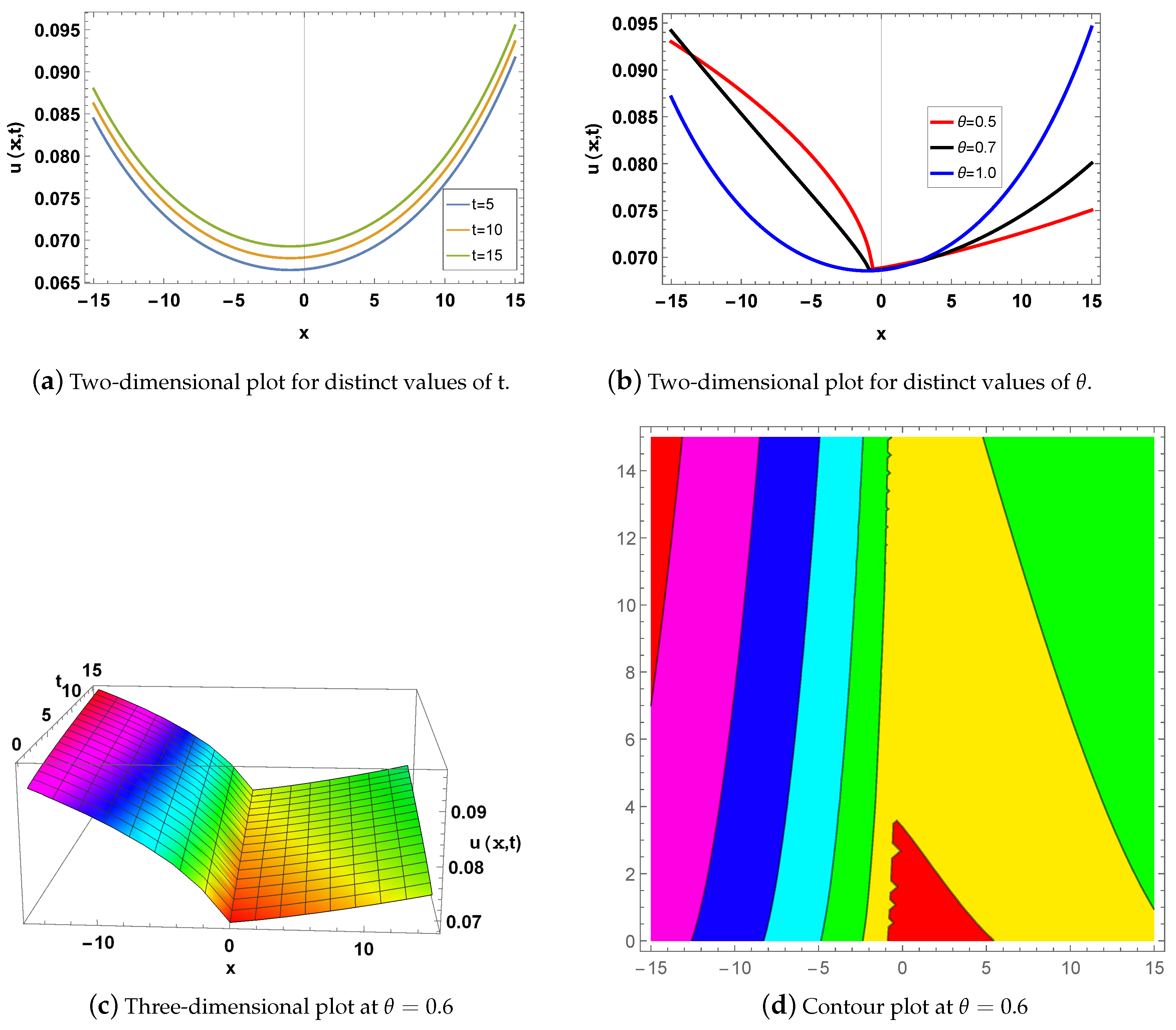
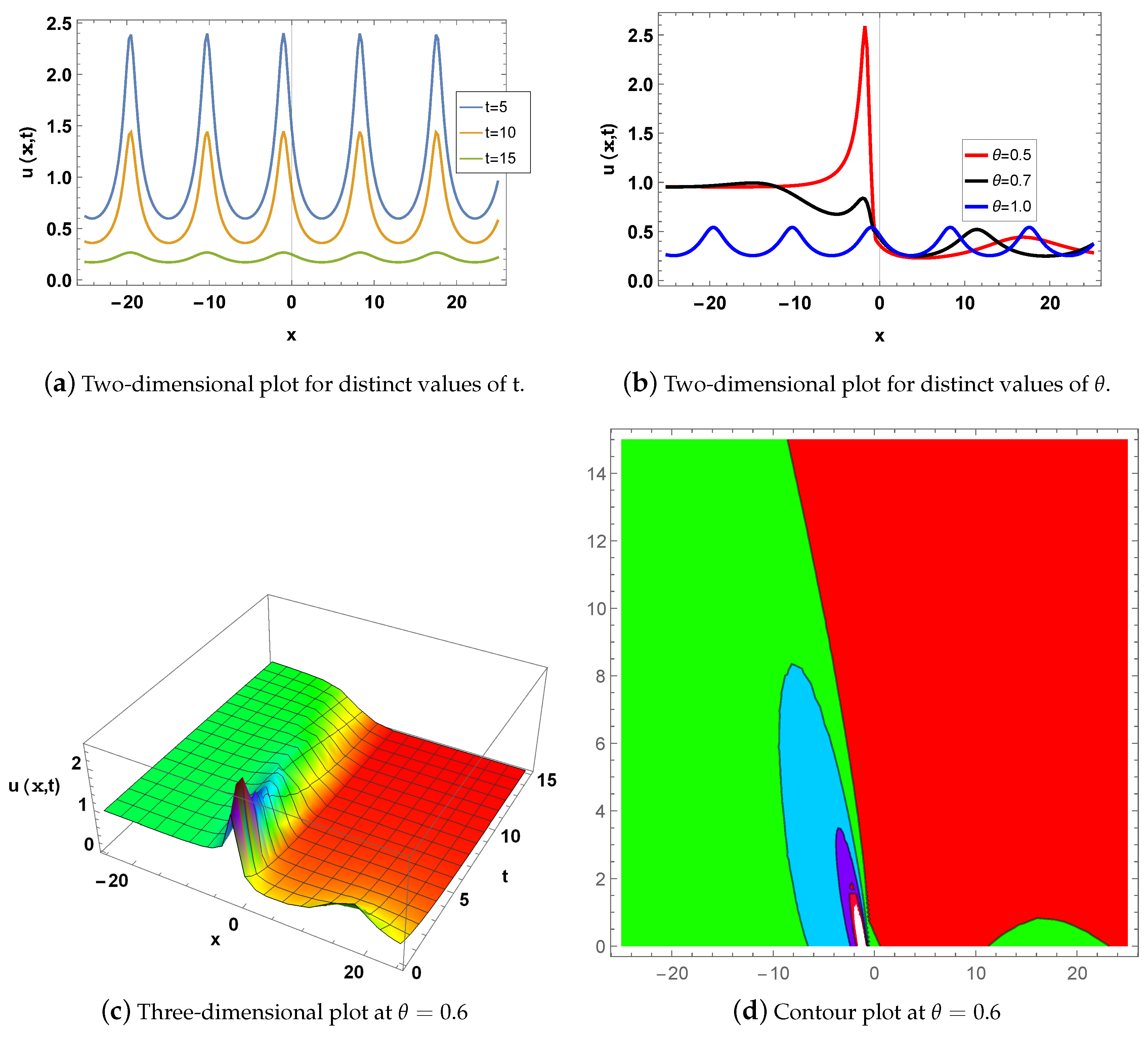
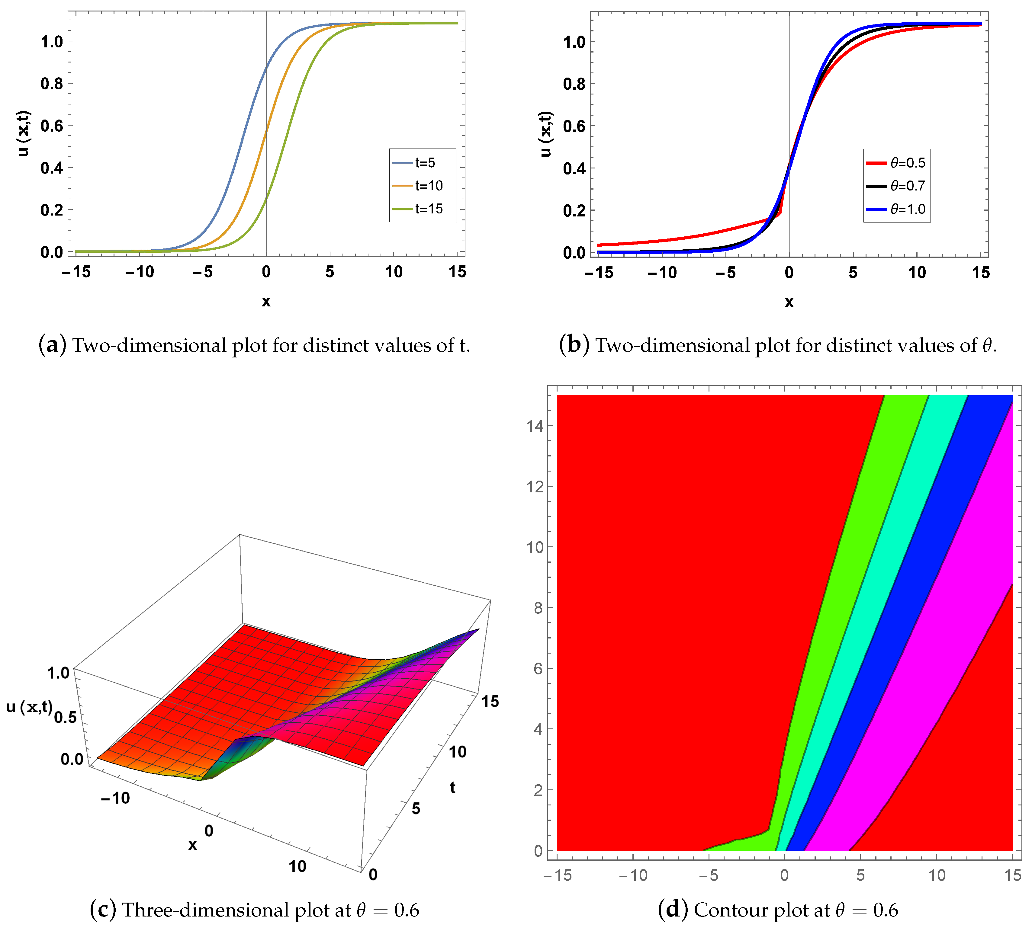
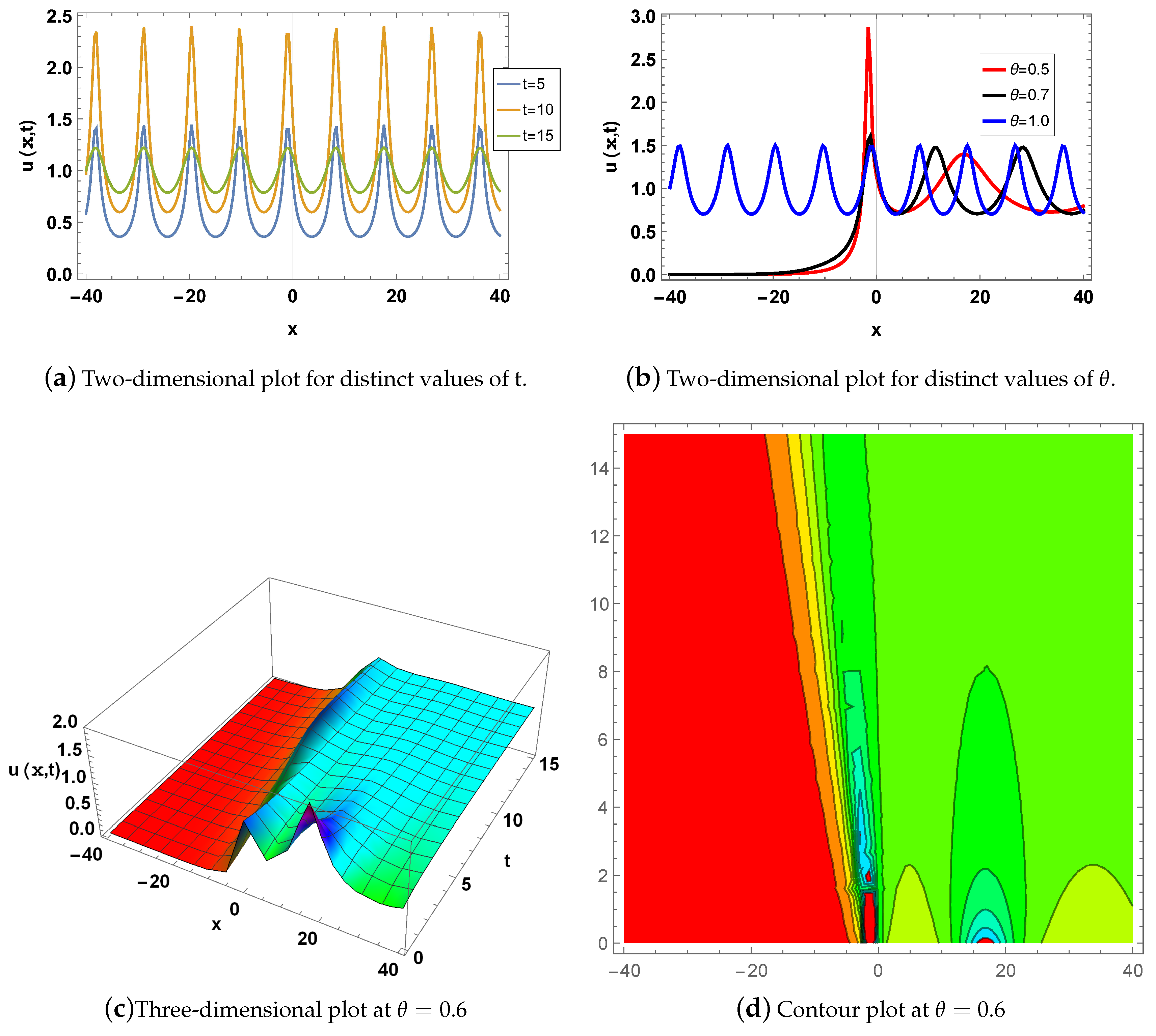
4. Graphical Description

In this section, the authors explain the attained results using two-dimensional, three-dimensional, and contour plots. The effect of the fractional derivative is also shown by representing graphs for $\theta =0.5$, $\theta =0.7$, and $\theta =1.0$.

5. Physical Interpretations

In this section, we will explain the physical behavior of some of the gained results to the beta-time fractional (1+1)-dimensional non-linear Van der Waals equation.

Figure 1 shows the dark wave solution for the values $\alpha =1.3$, $\beta =-0.03$, and $\delta =-0.8$. Figure 1a shows a 2-D plot for $-15<x<15$ when $\theta =1$, with a blue curve if t is 5, an orange curve if the value of t is 10, and a green curve if the value of t is 15. Figure 1b denotes a 2-dimensional graph for $-15<x<15$ and $t\in (5,15)$, while the red curve if $\theta =0.5$, the black curve if $\theta =0.7$, and the blue curve if $\theta =1$. Figure 1c shows a 3-D plot at $\theta =0.6$ with $t\in (5,15)$. Figure 1d denotes a contour graph at $\theta =0.6$ with $t\in (5,15)$. In all figures, we plotted the analytical solution in different times according to made procedures. These results enable us to can discover some features of dark wave solutions.

Figure 2 shows the singular wave solution for the values $\alpha =2.7$, $\beta =0.35$, and $\delta =-0.5$. Figure 2a shows a 2-D plot for $-25<x<25$ when $\theta =1$, with a blue curve if t is 5, an orange curve if the value of t is 10, and a green curve if the value of t is 15. Figure 2b denotes a 2-dimensional graph for $-25<x<25$ and $t\in (5,15)$, with a red curve if $\theta =0.5$, a black curve if $\theta =0.7$, and a blue curve if $\theta =1$. Figure 2c shows a 3-D plot at $\theta =0.6$ with $t\in (5,15)$. Figure 2d denotes a contour graph at $\theta =0.6$ with $t\in (5,15)$. In all figures, we plotted the analytical solution in different times according to made procedures. These results enable us to can discover some features of singular wave solutions.

Figure 3 shows the periodic wave solution for the values $\alpha =2.7$, $\beta =-0.45$, and $\delta =0.5$. Figure 3a shows a 2-D plot for $-15<x<15$ when $\theta =1$, with a blue curve if t is 5, an orange curve if the value of t is 10, and a green curve if the value of t is 15. Figure 3b denotes a 2-dimensional graph for $-15<x<15$ and $t\in (5,15)$, with a red curve if $\theta =0.5$, a black curve if $\theta =0.7$, and a blue curve if $\theta =1$. Figure 3c shows a 3-D plot at $\theta =0.6$ with $t\in (5,15)$. Figure 3d denotes a contour graph at $\theta =0.6$ with $t\in (5,15)$. In all figures, we plotted the analytical solution in different times according to made procedures. These results enable us to can discover some features of periodic wave solutions.

Figure 4 shows the singular-dark wave solution for the values $\alpha =2.7$, $\beta =0.35$, and $\delta =-0.2$. Figure 4a shows a 2-D plot for $-40<x<40$ when $\theta =1$, with a blue curve if t is 5, an orange curve if the value of t is 10, and a green curve if the value of t is 15. Figure 4b denotes a 2-dimensional graph for $-40<x<40$ and $t\in (5,15)$, with a red curve if $\theta =0.5$, a black curve if $\theta =0.7$, and a blue curve if $\theta =1$. Figure 4c shows a 3-D plot at $\theta =0.6$ with $t\in (5,15)$. Figure 4d denotes a contour graph at $\theta =0.6$ with $t\in (5,15)$. The parameter $\alpha$ denotes the viscosity effect; a high value of $\alpha$ makes the flow of fluids sluggishly, and a low value makes the flow of fluids more easily. This same behavior is also observed in our obtained results when we increase the value of $\alpha$, where we obtain the different curves of our results. In all figures, we plotted the analytical solution in different times according to made procedures. These results enable us to can discover some features of singular-dark wave solutions.

6. Stability Analysis

In this section, we will explain the stability of the governing system. This analysis is performed by using the Hamiltonian system, which is tested on a few of the obtained solutions to show the stability of the concerning system in different applications. Stability analyses have been performed for various models such as [81,82]. Here, we study the Equation (1) stability, for which we define the Hamiltonian transformation as

$$\begin{array}{c}\hfill \mathcal{M}={\displaystyle \frac{1}{2}}{\int }_{-\infty }^{\infty }{\mathit{u}}^{\mathit{2}}dx,\end{array}$$

(76)

where $\mathcal{M}$ represents the momentum factor and the possibility for power is represented by $\mathit{u}(\mathit{x},\mathit{t})$. Now, we give a necessary criterion of stable soliton solutions.

$$\begin{array}{c}\hfill {\displaystyle \frac{\partial \mathcal{M}}{\partial \omega }}>0,\end{array}$$

(77)

where $\omega$ represents a soliton velocity; putting Equation (22) into Equation (76) yields

$$\begin{array}{c}\mathcal{M}={\displaystyle \frac{1}{2}}{\int }_{-7}^7(\pm {\displaystyle \frac{\alpha \sqrt{\beta }}{\sqrt{18-4{\alpha }^2}}}\pm {\displaystyle \frac{\alpha \sqrt{2{\alpha }^2-9}\sqrt{\beta }}{(2{\alpha }^2-9)\sqrt{2\delta }}}(-\sqrt{-\delta }tanh(\sqrt{-\delta }({\displaystyle \frac{\alpha \sqrt{\beta }}{\sqrt{(8{\alpha }^2-36)\delta }}}x\hfill \\ \hfill -{\displaystyle \frac{3\alpha \beta }{2(2{\alpha }^2-9)\sqrt{-\delta }}}{t)))))}^{2}dx,\end{array}$$

(78)

By using the criterion is given in Equation (77), we obtain the following

$$\begin{array}{c}{\displaystyle \frac{1}{2}}((2\sqrt{2}\alpha \sqrt{\beta }\sqrt{(2{\alpha }^2-9)\delta }(\sqrt{-\delta }ttanh({\displaystyle \frac{1}{2}}\sqrt{-\delta }({\displaystyle \frac{2t(3\alpha \beta )}{2(2{\alpha }^2-9)\sqrt{-\delta }}}-{\displaystyle \frac{7\alpha \sqrt{\beta }}{\sqrt{(2{\alpha }^2-9)\delta }}}))\hfill \\ -\sqrt{-\delta }ttanh({\displaystyle \frac{1}{2}}\sqrt{-\delta }({\displaystyle \frac{7\alpha \sqrt{\beta }}{\sqrt{(2{\alpha }^2-9)\delta }}}+{\displaystyle \frac{2t(3\alpha \beta )}{2(2{\alpha }^2-9)\sqrt{-\delta }}}))))/(\sqrt{18-4{\alpha }^2}\sqrt{2{\alpha }^2-9}\sqrt{\delta })\\ +(\alpha \sqrt{\beta }\sqrt{(2{\alpha }^2-9)\delta }(\sqrt{-\delta }t{\sec \mathrm{h}}^2(\sqrt{-\delta }({\displaystyle \frac{t(-(3\alpha \beta ))}{2(2{\alpha }^2-9)\sqrt{-\delta }}}-{\displaystyle \frac{7\alpha \sqrt{\beta }}{2\sqrt{(2{\alpha }^2-9)\delta }}}))\\ \hfill -\sqrt{-\delta }t{\sec \mathrm{h}}^2(\sqrt{-\delta }({\displaystyle \frac{7\alpha \sqrt{\beta }}{2\sqrt{(2{\alpha }^2-9)\delta }}}-{\displaystyle \frac{t(3\alpha \beta )}{2(2{\alpha }^2-9)\sqrt{-\delta }}}))))/((2{\alpha }^2-9)\sqrt{-\delta }))>0.\end{array}$$

(79)

Hence, Equation (1) represents a stable nonlinear fractional model provided that the above condition is fulfilled.

7. Modulation Instability Analysis

Considering a steady-state solution of the (1 + 1)-dimensional non-linear Van der Waals equation is of the form [83],

$$u(x,t)=\left(U(x,t)+\sqrt{\tau }\right)e^{\iota \tau t},$$

(80)

where $\tau$ denotes the normalized optical power.

Putting Equation (80) into Equation (1). After linearizing, we obtain

$$-{\tau }^{5/2}+2\iota \tau U_t+U_{\mathrm{tt}}-{\tau }^{2}U-\alpha \iota \tau U_{\mathrm{xx}}-\beta U_{\mathrm{xx}}-\alpha U_{\mathrm{xxt}}+U_{\mathrm{xxxx}}=0.$$

(81)

Assuming the result of the Equation (81) given as

$$U(x,t)=A_1{e}^{\iota (px-qt)}+A_2{e}^{-\iota (px-qt)},$$

(82)

where p and q denote the frequency and normalized wave number of perturbation, respectively. We substitute Equation (82) into Equation (81). By collecting the coefficients of $e^{\iota (px-qt)}$ and $e^{\iota (px-qt)}$, we obtain the dispersion relation after solving the determinant of the coefficient matrix.

$$p^8+2\beta p^6-{\alpha }^2{p}^4{\tau }^2+{\beta }^2{p}^4+{\alpha }^2{p}^4{q}^2-2p^4{q}^2-2p^4{\tau }^2-2\beta p^2{\tau }^2-2\beta p^2{q}^2+q^4-2q^2{\tau }^2+{\tau }^4=0=0.$$

(83)

Determine the dispersion relation from Equation (83) for q, which yields

$$q=\pm \sqrt{-{\displaystyle \frac{1}{2}}{\alpha }^2{p}^4+p^4+\beta p^2+{\displaystyle \frac{1}{2}}\sqrt{{\alpha }^4{p}^8-4{\alpha }^2{p}^8-4{\alpha }^2\beta p^6+16p^4{\tau }^2+16\beta p^2{\tau }^2}+{\tau }^2}.$$

(84)

The gained dispersion relation shows steady-state stability. When a wave number q is imaginary, then steady-state the result will be unstable since the perturbation increases exponentially. But when a wave number q is real, then the steady state is converted into stability against small perturbations. The steady-state result is unstable if

$$p^4-{\displaystyle \frac{1}{2}}{\alpha }^2{p}^4+\beta p^2+{\displaystyle \frac{1}{2}}\sqrt{{\alpha }^4{p}^8-4{\alpha }^2{p}^8-4{\alpha }^2\beta p^6+16p^4{\tau }^2+16\beta p^2{\tau }^2}+{\tau }^2<0.$$

(85)

The modulation instability (MI) gain spectrum $G(p)$ is obtained as

$$G(p)=2Im(q)=\pm \sqrt{p^4-{\displaystyle \frac{1}{2}}{\alpha }^2{p}^4+\beta p^2+{\displaystyle \frac{1}{2}}\sqrt{{\alpha }^4{p}^8-4{\alpha }^2{p}^8-4{\alpha }^2\beta p^6+16p^4{\tau }^2+16\beta p^2{\tau }^2}+{\tau }^2}.$$

(86)

The gained dispersion is provided and presented in Figure 5 to investigate the steady-state stability.

8. Conclusions

This paper contains the distinct types of exact soliton solutions of the (1 + 1)-dimensional non-linear Van der Waals equation along the beta-time fractional derivative. We obtain bright, dark, dark-solitary, dark-singular, periodic wave, and many more exact wave solutions by using the modified extended tanh function method. The use of fractional derivatives makes the solutions different from the existing solutions. The obtained results are represented by two-dimensional, three-dimensional, and contour graphs. Stability analysis is carried out to check the stability of the model. Additionally, modulation instability is performed to study the stationary solutions of the governing model. Results are helpful in the progress of the concerned system. The gained results will be of high importance in the interaction of quantum-mechanical fluctuations, granular matters, and other fields of Van der Waals equation applications. The achieved results are also useful in various naturally occurring phenomena, industries, geophysics, civil engineering, pharmaceutical, and many others. It is suggested that the method used is also useful for the other nonlinear models of different fields of science and engineering.

References

1. Seadawy, A.R.; Ali, A.; Bekir, A. Exact wave solutions of new generalized Bogoyavlensky–Konopelchenko model in fluid mechanics. Mod. Phys. Lett. B 2024, 38, 2450262. [Google Scholar] [CrossRef]
2. Durur, H. Exact Solutions of the Oskolkov Equation in Fluid Dynamics. Afyon Kocatepe Univ. J. Sci. Eng. 2023, 2, 355–361. [Google Scholar] [CrossRef]
3. Dehghan, M.; Manafian, J.; Saadatmandi, A. Solving nonlinear fractional partial differential equations using the homotopy analysis method. Numer. Methods Partial. Differ. Equ. J. 2010, 26, 448–479. [Google Scholar] [CrossRef]
4. Dehghan, M.; Manafian, J. The solution of the variable coefficients fourth–order parabolic partial differential equations by homotopy perturbation method. Z. Naturforsch. A 2009, 64a, 420–430. [Google Scholar] [CrossRef]
5. Seadawy, A.R.; Manafian, J. New soliton solution to the longitudinal wave equation in a magneto-electro-elastic circular rod. Results Phys. 2018, 8, 1158–1167. [Google Scholar] [CrossRef]
6. Ullah, M.S.; Abdeljabbar, A.; Roshid, H.-O.; Ali, M.Z. Application of the unified method to solve the Biswas–Arshed model. Results Phys. 2022, 42, 105946. [Google Scholar] [CrossRef]
7. Aydemir, T. Application of the generalized unified method to solve (2 + 1)-dimensional Kundu–Mukherjee–Naskar equation. Opt. Quantum Electron. 2023, 55, 534. [Google Scholar] [CrossRef]
8. Batiha, I.M.; Njadat, S.A.; Batyha, R.M.; Zraiqat, A.; Dababneh, A.; Momani, S. Design Fractional-order PID Controllers for Single-Joint Robot Arm Model. Int. J. Adv. Soft Comput. Its Appl. 2022, 14, 96–114. [Google Scholar] [CrossRef]
9. Ahmad, S.; Mahmoud, E.E.; Saifullah, S.; Ullah, A.; Ahmad, S.; Akgül, A.; El Din, S.M. New waves solutions of a nonlinear Landau–Ginzburg–Higgs equation: The Sardar-subequation and energy balance approaches. Results Phys. 2023, 51, 106736. [Google Scholar] [CrossRef]
10. Jiang, H.; Li, S.M.; Wang, W.G. Moderate deviations for parameter estimation in the fractional ornstein-uhlenbeck processes with periodic mean. Acta Math. Sin. Engl. Ser. 2024, 40, 1308–1324. [Google Scholar] [CrossRef]
11. Chen, D.; Zhao, T.; Han, L.; Feng, Z. Single-stage multi-input buck type high-frequency link’s inverters with series and simultaneous power supply. IEEE Trans. Power Electron. 2022, 37, 7411–7421. [Google Scholar] [CrossRef]
12. Xie, G.; Fu, B.; Li, H.; Du, W.; Zhong, Y.; Wang, L.; Geng, H.; Zhang, J.; Si, L. A gradient-enhanced physics-informed neural networks method for the wave equation. Eng. Anal. Boundary Elements 2024, 166, 105802. [Google Scholar] [CrossRef]
13. Li, X.; Hu, S.; He, J.; Li, D.; Xi, Y.; Lan, H.L.; Xu, L.; Mingliang Tan, M.; Xiao, M. Electric-feld-driven printed 3D highly ordered microstructure with cell feature size promotes the maturation of engineered cardiac tissues. Adv. Sci. 2023, 10, 2206264. [Google Scholar]
14. Zhang, K.; Liu, Q.; Qian, H.; Xiang, B.; Cui, Q.; Zhou, J.; Chen, E. Eatn: An efficient adaptive transfer network for aspect-level sentiment analysis. IEEE Trans. Knowl. Data Eng. 2021, 35, 377–389. [Google Scholar] [CrossRef]
15. Chen, D.; Zhao, T.; Xu, S. Single-stage multi-input buck type high-frequency link’s inverters with multiwinding and time-sharing power supply. IEEE Trans. Power Elec. 2022, 37, 12763–12773. [Google Scholar] [CrossRef]
16. Chen, C.; Han, D.; Chang, C.C. MPCCT: Multimodal vision-language learning paradigm with context-based compact transformer. Pattern Recogn. 2024, 147, 110084. [Google Scholar] [CrossRef]
17. Shi, S.; Han, D.; Cui, M. A multimodal hybrid parallel network intrusion detection model. Connect. Sci. 2023, 35, 2227780. [Google Scholar] [CrossRef]
18. Wanh, H.; Han, D.; Cui, M.; Chen, C. NAS-YOLOX: A SAR ship detection using neural architecture search and multi-scale attention. Connect. Sci. 2023, 35, 1–32. [Google Scholar]
19. Zhou, C.; Wang, C.; Zhang, B.; Li, B. Deep Learning-Based Coseismic Deformation Estimation From InSAR Interferograms. IEEE Trans. Geosci. Remote Sens. 2024, 62, 5203610. [Google Scholar] [CrossRef]
20. Fei, R.; Guo, Y.; Li, J.; Hu, B.; Yang, L. An improved BPNN method based on probability density for indoor location. IEICE Trans. Inf. Syst. 2023, 106, 773–785. [Google Scholar] [CrossRef]
21. Mohammed, P.O.; Agarwal, R.P.; Brevik, I.; Abdelwahed, M.; Kashuri, A.; Yousif, M.A. On Multiple-Type Wave Solutions for the Nonlinear Coupled Time-Fractional Schrödinger Model. Symmetry 2024, 16, 553. [Google Scholar] [CrossRef]
22. Ozkan, E.M. New exact solutions of some important nonlinear fractional partial differential Equations with beta derivative. Fractal Fract. 2022, 6, 173. [Google Scholar] [CrossRef]
23. Qawaqneh, H.; Zafar, A.; Raheel, M.; Zaagan, A.A.; Zahran, E.H.M.; Cevikel, A.; Bekir, A. New soliton solutions of M-fractional Westervelt model in ultrasound imaging via two analytical techniques. Opt. Quantum Electron. 2024, 56, 737. [Google Scholar] [CrossRef]
24. Gasmi, B.; Moussa, A.; Mati, Y.; Alhakim, L.; Baskonus, H.M. Bifurcation and exact traveling wave solutions to a conformable nonlinear Schrödinger equation using a generalized double auxiliary equation method. Opt. Quantum Electron. 2024, 56, 18. [Google Scholar] [CrossRef]
25. Faridi, W.A.; Myrzakulova, Z.; Myrzakulov, R.; Akgül, A.; Osman, M.S. The construction of exact solution and explicit propagating optical soliton waves of Kuralay equation by the new extended direct algebraic and Nucci’s reduction techniques. Int. J. Modell. Simul. 2024, 1–20. [Google Scholar] [CrossRef]
26. Nasreen, N.; Rafiq, M.N.; Younas, U.; Arshad, M.; Abbas, M.; Ali, M.R. Stability analysis and dynamics of solitary wave solutions of the (3+ 1)-dimensional generalized shallow water wave equation using the Ricatti equation mapping method. Results Phys. 2024, 56, 107226. [Google Scholar] [CrossRef]
27. Faridi, W.A.; Wazwaz, A.-M.; Mostafa, A.M.; Myrzakulov, R.; Umurzakhova, Z. The Lie point symmetry criteria and formation of exact analytical solutions for Kairat-II equation: Paul-Painlevé approach, Chaos. Solitons Fractals 2024, 182, 114745. [Google Scholar] [CrossRef]
28. Wang, H. Exact traveling wave solutions of the generalized fifth-order dispersive equation by the improved Fan subequation method. Math. Methods Appl. Sci. 2024, 47, 1701–1710. [Google Scholar] [CrossRef]
29. Arnous, A.H.; Hashemi, M.S.; Nisar, K.S.; Shakeel, M.; Ahmad, J.; Ahmad, I.; Jan, R.; Ali, A.; Kapoor, M.; Shah, N.A. Investigating solitary wave solutions with enhanced algebraic method for new extended Sakovich equations in fluid dynamics. Results Phys. 2024, 57, 107369. [Google Scholar] [CrossRef]
30. Ramya, S.; Krishnakumar, K.; Ilangovane, R. Exact solutions of time fractional generalized burgers–Fisher equation using exp and exponential rational function methods. Int. J. Dyn. Control 2024, 12, 292–302. [Google Scholar] [CrossRef]
31. Eidinejad, Z.; Saadati, R.; Li, C.; Inc, M.; Vahidi, J. The multiple exp-function method to obtain soliton solutions of the conformable Date–Jimbo–Kashiwara–Miwa equations. Int. J. Mod. Phys. B 2024, 38, 2450043. [Google Scholar] [CrossRef]
32. Feng, Y.; Bilige, S. Multiple rogue wave solutions of (2 + 1)-dimensional YTSF equation via Hirota bilinear method. Waves Random Complex Medium 2024, 34, 94–110. [Google Scholar] [CrossRef]
33. Elsadany, A.A.; Elboree, M.K. Construction of shock, periodic and solitary wave solutions for fractional-time Gardner equation by Jacobi elliptic function method. Opt. Quantum Electron. 2024, 56, 481. [Google Scholar] [CrossRef]
34. Eslami, M.; Heidari, S.; Abduridha, S.A.J.; Asghari, Y. Dynamic simulation of traveling wave solutions for the differential-difference Burgers’ equation utilizing a generalized exponential rational function approach. Opt. Quantum Electron. 2024, 56, 504. [Google Scholar] [CrossRef]
35. Khan, M.I.; Farooq, A.; Nisar, K.S.; Shah, N.A. Unveiling new exact solutions of the unstable nonlinear Schrödinger equation using the improved modified Sardar sub-equation method. Results Phys. 2024, 59, 107593. [Google Scholar] [CrossRef]
36. Samir, I.; Ahmed, H.M.; Darwish, A.; Hussein, H.H. Dynamical behaviors of solitons for NLSE with Kudryashov’s sextic power-law of nonlinear refractive index using improved modified extended tanh-function method. Ain Shams Eng. J. 2024, 15, 102267. [Google Scholar] [CrossRef]
37. Ullah, N.; Asjad, M.I.; Awrejcewicz, J.; Muhammad, T.; Baleanu, D. On soliton solutions of fractional-order nonlinear model appears in physical sciences. AIMS Math. 2022, 7, 7421–7440. [Google Scholar] [CrossRef]
38. Luo, N.; Peng, Z.; Hu, J.; Ghosh, B.K. Adaptive optimal control of affine nonlinear systems via identifier-critic neural network approximation with relaxed PE conditions. Neural Netw. 2023, 167, 588–600. [Google Scholar] [CrossRef] [PubMed]
39. Zhu, C.; Al-Dossari, M.; Rezapour, S.; Alsallami, S.A.M.; Gunay, B. Bifurcations, chaotic behavior, and optical solutions for the complex Ginzburg-Landau equation. Results Phys. 2024, 59, 107601. [Google Scholar] [CrossRef]
40. Zhu, C.; Al-Dossari, M.; Rezapour, S.; Gunay, B. On the exact soliton solutions and different wave structures to the (2+1) dimensional Chaffee-Infante equation. Results Phys. 2024, 57, 107431. [Google Scholar] [CrossRef]
41. Zhu, C.; Al-Dossari, M.; Rezapour, S.; Shateyi, S.; Gunay, B. Analytical optical solutions to the nonlinear Zakharov system via logarithmic transformation. Results Phys. 2024, 56, 107298. [Google Scholar] [CrossRef]
42. Kai, Y.; Ji, J.; Yin, Z. Study of the generalization of regularized long-wave equation. Nonlinear Dyn. 2022, 107, 2745–2752. [Google Scholar] [CrossRef]
43. Kai, Y.; Yin, Z. Linear structure and soliton molecules of Sharma-Tasso-Olver-Burgers equation. Phys. Let. A 2022, 452, 128430. [Google Scholar] [CrossRef]
44. Ali, T.A.A.; Xiao, Z.; Jiang, H.; Li, B. A Class of Digital Integrators Based on Trigonometric Quadrature Rules. IEEE Trans. Indus. Elec. 2024, 71, 6128–6138. [Google Scholar] [CrossRef]
45. Mohammadzadeh, A.; Taghavifar, H.; Zhang, Y.; Zhang, W. A Fast Nonsingleton Type-3 Fuzzy Predictive Controller for Nonholonomic Robots Under Sensor and Actuator Faults and Measurement Errors. IEEE Trans. Syst. Man Cybern. Syst. 2024, 54, 4175–4187. [Google Scholar] [CrossRef]
46. Mohammadzadeh, A.; Zhang, C.; Alattas, K.A.; El-Sousy, F.F.; Vu, M.T. Fourier-based type-2 fuzzy neural network: Simple and effective for high dimensional problems. Neurocomput. 2023, 547, 126316. [Google Scholar] [CrossRef]
47. Mohammadzadeh, A.; Taghavifar, H.; Zhang, C.; Alattas, K.A.; Liu, J.; Vu, M.T. A non-linear fractional-order type-3 fuzzy control for enhanced path-tracking performance of autonomous cars. IET Control Theo. Appl. 2024, 18, 40–54. [Google Scholar] [CrossRef]
48. Yan, S.R.; Guo, W.; Mohammadzadeh, A.; Rathinasamy, S. Optimal deep learning control for modernized microgrids. Appl. Intelligence 2023, 53, 15638–15655. [Google Scholar] [CrossRef]
49. Hui, Z.; Wu, A.; Han, D.; Li, T.; Li, L.; Gong, J.; Li, X. Switchable Single- to Multiwavelength Conventional Soliton and Bound-State Soliton Generated from a NbTe2 Saturable Absorber-Based Passive Mode-Locked Erbium-Doped Fiber Laser. ACS Appl. Mater. Interfaces 2024, 16, 22344–22360. [Google Scholar] [CrossRef]
50. Gong, S.P.; Khishe, M.; Mohammadi, M. Niching chimp optimization for constraint multimodal engineering optimization problems. Expert Sys. Appl. 2022, 198, 116887. [Google Scholar] [CrossRef]
51. Chen, F.; Yang, C.; Khishe, M. Diagnose parkinson’s disease and cleft lip and palate using deep convolutional neural networks evolved by ip-based chimp optimization algorithm. Biomed. Signal Proc. Cont. 2022, 77, 103688. [Google Scholar] [CrossRef]
52. Shi, W.; Zhou, C.; Zhang, Y.; Li, K.; Ren, X.; Liu, H.; Ye, X. Hybrid modeling on reconstitution of continuous arterial blood pressure using finger photoplethysmography Biomed. Signal Proc. Cont. 2023, 85, 2023. [Google Scholar]
53. Alazeb, A.; Chughtai, B.R.; Al Mudawi, N.; AlQahtani, Y.; Alonazi, M.; Aljuaid, H.; Jalal, A.; Liu, H. Remote intelligent perception system for multi-object detection Front. Neurorobotics 2024, 18, 1398703. [Google Scholar] [CrossRef] [PubMed]
54. Bo, Q.; Cheng, W.; Khishe, M.; Mohammadi, M.; Mohammed, A.H. Solar photovoltaic model parameter identification using robust niching chimp optimization. Solar Energy 2022, 239, 179–197. [Google Scholar] [CrossRef]
55. Khishe, M. Greedy opposition-based learning for chimp optimization algorithm. Artif. Intell. Rev. 2023, 56, 7633–7663. [Google Scholar] [CrossRef]
56. Cai, C.F.; Gou, B.; Khishe, M.; Mohammadi, M.; Rashidi, S.; Moradpour, R.; Mirjalili, S. Improved deep convolutional neural networks using chimp optimization algorithm for covid19 diagnosis from the x-ray images. Expert Syst. Appl. 2023, 213, 119206. [Google Scholar] [CrossRef]
57. Khishe, M.; Orouji, N.; Mosavi, M.R. Multi-objective chimp optimizer: An innovative algorithm for multi-objective problems. Expert Syst. Appl. 2023, 211, 118734. [Google Scholar] [CrossRef]
58. Chen, C.; Han, D.; Shen, X. CLVIN: Complete language-vision interaction network for visual question answering. Knowl. Based Syst. 2023, 275, 110706. [Google Scholar] [CrossRef]
59. Chen, X.; Yang, P.; Wang, M.; Hu, F.; Xu, J. Output voltage drop and input current ripple suppression for the pulse load power supply using virtual multiple quasi-notch-flters impedance. IEEE Trans. Power Electron. 2023, 38, 9552–9565. [Google Scholar] [CrossRef]
60. Han, D.; Zhou, H.X.; Weng, T.H.; Wu, Z.; Han, B.; Li, K.C.; Pathan, A.S.K. LMCA: A lightweight anomaly network traffic detection model integrating adjusted mobilenet and coordinate attention mechanism for IoT. Telecommun. Syst. 2023, 84, 549–564. [Google Scholar] [CrossRef]
61. Liao, L.; Guo, Z.; Gao, Q.; Wang, Y.; Yu, F.; Zhao, Q.; Maybank, S.J.; Liu, Z.; Li, C.; Li, L. Color image recovery using generalized matrix completion over higher-order finite dimensional algebra. Axioms 2023, 12, 954. [Google Scholar] [CrossRef]
62. Meng, S.; Meng, F.; Chi, H.; Chen, H.; Pang, A. A robust observer based on the nonlinear descriptor systems application to estimate the state of charge of lithium-ion batteries. J. Frankl. Inst. 2023, 360, 11397–11413. [Google Scholar] [CrossRef]
63. Chen, D.L.; Zhao, J.W.; Qin, S.R. SVM strategy and analysis of a three-phase quasi-Z-source inverter with high voltage transmission ratio. Sci. China Technol. Sci. 2023, 66, 29963010. [Google Scholar] [CrossRef]
64. Liu, Z.; Xu, Z.; Zheng, X.; Zhao, Y.; Wang, J. 3D path planning in threat environment based on fuzzy logic. J. Intell. Fuzzy Sys. 2024, 46, 7021–7034. [Google Scholar] [CrossRef]
65. Hussein, H.H.; Ahmed, H.M.; Alexan, W. Analytical soliton solutions for cubic-quartic perturbations of the Lakshmanan-Porsezian-Daniel equation using the modified extended tanh function method. Ain Shams Eng. J. 2024, 15, 102513. [Google Scholar] [CrossRef]
66. Akbulut, A.; Taşcan, F. Application of conservation theorem and modified extended tanh-function method to (1+ 1)-dimensional nonlinear coupled Klein–Gordon–Zakharov equation, Chaos. Solitons Fractals 2017, 104, 33–40. [Google Scholar] [CrossRef]
67. Zahran, E.H.M.; Khater, M.M.A. Modified extended tanh-function method and its applications to the Bogoyavlenskii equation. Appl. Math. Modell. 2016, 40, 1769–1775. [Google Scholar] [CrossRef]
68. El-Wakil, S.A.; Abdou, M.A. Modified extended tanh-function method for solving nonlinear partial differential equations, Chaos. Solitons Fractals 2007, 31, 1256–1264. [Google Scholar] [CrossRef]
69. Zaman, U.H.M.; Arefin, M.A.; Akbar, M.A.; Uddin, M.H. Utilizing the extended tanh-function technique to scrutinize fractional order nonlinear partial differential equations. Partial Differ. Equ. Appl. Math. 2023, 8, 100563. [Google Scholar] [CrossRef]
70. Chu, Y.; Shallal, M.A.; Mirhosseini-Alizamini, S.M.; Rezazadeh, H.; Javeed, S.; Baleanu, D. Application of modified extended Tanh technique for solving complex Ginzburg-Landau equation considering Kerr law nonlinearity. Comput. Mater. Contin. 2021, 66, 1369–1378. [Google Scholar] [CrossRef]
71. Alam, L.M.B.; Jiang, X.; Al-Mamun, A. Exact and explicit traveling wave solution to the time-fractional phi-four and (2 + 1) dimensional CBS equations using the modified extended tanh-function method in mathematical physics. Partial Differ. Equ. Appl. Math. 2021, 4, 100039. [Google Scholar] [CrossRef]
72. Rabie, W.B.; Ahmed, H.M.; Darwish, A.; Hussein, H.H. Construction of new solitons and other wave solutions for a concatenation model using modified extended tanh-function method. Alex. Eng. J. 2023, 74, 445–451. [Google Scholar] [CrossRef]
73. Atangana, A.; Baleanu, D.; Alsaedi, A. Analysis of time-fractional Hunter–Saxton equation: A model of neumatic liquid crystal. Open Phys. 2016, 14, 145–149. [Google Scholar] [CrossRef]
74. Uddin, M.F.; Hafez, M.G.; Hammouch, Z.; Baleanu, D. Periodic and rogue waves for Heisenberg models of ferromagnetic spin chains with fractional beta derivative evolution and obliqueness. Waves Random Complex Media 2021, 31, 2135–2149. [Google Scholar] [CrossRef]
75. Ghanbari, B.; Gómez-Aguilar, J.F. The generalized exponential rational function method for Radhakrishnan–Kundu–Lakshmanan equation with Beta time derivative. Rev. Mex. Fís. 2019, 65, 503–518. [Google Scholar] [CrossRef]
76. Altalbe, A.; Zaagan, A.A.; Bekir, A.; Cevikel, A. The nonlinear wave dynamics of the space-time fractional van der Waals equation via three analytical methods. Phys. Fluids 2024, 36, 2. [Google Scholar] [CrossRef]
77. Bibi, S.; Ahmed, N.; Khan, U.; Mohyud-Din, S.T. Some new exact solitary wave solutions of the van der Waals model arising in nature. Results Phys. 2018, 9, 648–655. [Google Scholar] [CrossRef]
78. Zafar, A.; Mushtaq, T.; Malik, A.; Bekir, A. New solitary wave and other exact solutions of the van der Waals normal form for granular materials. J. Ocean Eng. Sci. 2022, 7, 170–177. [Google Scholar] [CrossRef]
79. Ali, N.H.; Mohammed, S.A.; Manafian, J. New explicit soliton and other solutions of the Van der Waals model through the EShGEEM and the IEEM. J. Modern Tech. Eng. 2023, 8, 5–18. [Google Scholar]
80. Raslan, K.R.; Khalid, K.A.; Shallal, M.A. The modified extended tanh method with the Riccati equation for solving the space-time fractional EW and MEW equations, Chaos. Solitons Fractals 2017, 103, 404–409. [Google Scholar] [CrossRef]
81. Tariq, K.U.; Wazwaz, A.M.; Javed, R. Construction of different wave structures, stability analysis and modulation instability of the coupled nonlinear Drinfel–Sokolov–Wilson model, Chaos. Solitons Fractals 2023, 166, 112903. [Google Scholar] [CrossRef]
82. Zulfiqar, H.; Aashiq, A.; Tariq, K.U.; Ahmad, H.; Almohsen, B.; Aslam, M.; Rehman, H.U. On the solitonic wave structures and stability analysis of the stochastic nonlinear Schrödinger equation with the impact of multiplicative noise. Optik 2023, 289, 171250. [Google Scholar] [CrossRef]
83. Ur Rehman, S.; Ahmad, J. Modulation instability analysis and optical solitons in birefringent fibers to RKL equation without four wave mixing. Alex. Eng. J. 2021, 60, 1339–1354. [Google Scholar] [CrossRef]
Figure 1. Plots for | u ( x , t ) | , represented by Equation (22), in 2-dimensional, 3-dimensional, and contour plots.
Mathematics 12 02257 g001
Figure 2. Plots for | u ( x , t ) | , represented by Equation (23), in 2-dimensional, 3-dimensional, and contour plots.
Mathematics 12 02257 g002
Figure 3. Plots for | u ( x , t ) | , represented by Equation (24), in 2-dimensional, 3-dimensional, and contour plots.
Mathematics 12 02257 g003
Figure 4. Plot for | u ( x , t ) | , represented by Equation (57), in 2-dimensional, 3-dimensional, and contour plots.
Mathematics 12 02257 g004
Figure 5. Gain spectrum of modulation instability (MI) for distinct values of p.
Mathematics 12 02257 g005
Disclaimer/Publisher’s Note: The statements, opinions and data contained in all publications are solely those of the individual author(s) and contributor(s) and not of MDPI and/or the editor(s). MDPI and/or the editor(s) disclaim responsibility for any injury to people or property resulting from any ideas, methods, instructions or products referred to in the content.