
From Classical to Modern Nonlinear Central Limit Theorems

1
Faculty of Computer Science, HSE University, 109028 Moscow, Russia
2
Faculty of Computational Mathematics and Cybernetics, Lomonosov Moscow State University, 119991 Moscow, Russia
Mathematics 2024, 12(14), 2276; https://doi.org/10.3390/math12142276
Submission received: 7 June 2024
/
Revised: 18 July 2024
/
Accepted: 18 July 2024
/
Published: 21 July 2024
(This article belongs to the Special Issue New Trends in Stochastic Processes, Probability and Statistics)
Abstract
:In 1733, de Moivre, investigating the limit distribution of the binomial distribution, was the first to discover the existence of the normal distribution and the central limit theorem (CLT). In this review article, we briefly recall the history of classical CLT and martingale CLT, and introduce new directions of CLT, namely Peng’s nonlinear CLT and Chen–Epstein’s nonlinear CLT, as well as Chen–Epstein’s nonlinear normal distribution function.
MSC:
60F05; 60-031. Introduction
The central limit theorem (CLT) is one of the gems of probability theory. Its importance can hardly be overestimated both from the theoretical point of view and from the point of view of its applications in various fields. The CLT is usually associated with the normal distribution, or Gaussian distribution, which acts as the limiting distribution in the theorem. In this review article, we recall the history of the CLT, briefly focusing on classical and martingale CLTs and discussing the newer directions of CLT, namely Peng’s nonlinear CLT and Chen–Epstein’s nonlinear CLT, in more detail, as well as the Chen–Epstein nonlinear normal distribution.
Speaking of the classical and martingale CLTs, we only touch upon the basic results involving the de Moivre–Laplace theorem, the Lindeberg–Feller theorem, the Lévy theorem and Hall’s theorem. We point out that the classical CLT is related to sums of independent random variables. In the martingale CLT, the summands are already dependent. But, in both cases, we consider a linear expectation and a probability space with one probability measure. This part of the review is rather short, since there are numerous publications on classical and martingale CLTs. A detailed and extensive review of the classical and martingale CLTs can be found in Rootzén [1], Hall and Heyde [2], Adams [3], and Fischer [4]. Further research was carried out in several directions, including the rates of convergance, see, e.g., Petrov [5], Götze et al. [6], Shevtsova [7], Fujikoshi and Ulyanov [8], and Dedecker et al. [9]; generalization of CLT to the multivariate case, see, e.g., Bhattacharya and Ranga Rao [10] and Sazonov [11], and to infinite dimensional case, see, e.g., Bentkus and Götze [12], Götze and Zaitsev [13], and Prokhorov and Ulyanov [14].
The main part of the paper is devoted to the nonlinear CLT. The motivation for its emergence comes from real life, where we often face decision-making problems under uncertainty. In most cases, classical CLT and normal distribution are not suitable. For example, we cannot directly construct a confidence interval using the martingale CLT. Nonlinear probability and expectation theory has developed rapidly over the last thirty years and has become an important tool for investigating model uncertainty or ambiguity. Nonlinear CLT is an important research area that describes the asymptotic behavior of a sequence of random variables with distribution uncertainty. Its limiting distribution is no longer represented by the classical normal distribution, but by a number of “new nonlinear normal distributions”, such as the g-expectation distribution and the G-normal distribution. Nonlinear CLT can fill the huge gaps between martingale CLT and real life.
Nonlinear CLT can be applied in many areas. For example, two-sample tests analyze whether the difference between two population parameters is more significant than a given positive equivalence margin. Chen et al. [15] developed a strategy-specific test statistic using nonlinear CLT and the law of large numbers. Furthermore, inspired by the nonlinear CLT and sublinear expectation theory, Peng et al. [16] introduced G-VaR, which is a new methodology for financial risk management. The inherent volatility of financial returns is not restricted to a single distribution; instead, it is reflected by an infinite set of distributions. By carefully assessing the most unfavorable scenario in this spectrum of possibilities, the G-VaR predictor can be accurately determined; see also Hölzermann [17] on pricing interest rate derivatives under volatility uncertainty and Ji et al. [18] on imbalanced binary classification under distribution uncertainty.
This paper is organised as follows: in Section 2, we consider the classical CLT. Section 3 presents the CLT for martingales. Section 4 introduces the theory of nonlinear expectations and nonlinear CLT. In Section 5, we discuss the differences between classical CLT and nonlinear CLT. Section 6 presents some future research problems of nonlinear CLT.
2. The Classical Central Limit Theorems
The first version of the CLT appeared as the de Moivre–Laplace theorem. De Moivre’s investigation was motivated by a need to compute the probabilities of winning in various games of chance. In the proof, de Moivre [19] used Stirling’s formula to obtain the following theorem.
Theorem 1
(de Moivre (1733) [19]). Let be a sequence of independent Bernoulli random variables, each with a success probability ; that is, for each i,
Let denote the total number of successes in the first n Bernoulli trials. Then, for any ,
where
is the standard normal distribution function.
Thus, de Moivre discovered the probability distribution, which, in the late 19th century, came to be called the normal distribution. Another name—Gaussian distribution—is used in honor of Gauss, who arrived at this distribution as ‘‘the law of error’’ in his famous work, Gauss [20], on the problems of measurement in astronomy and the least squares method.
Laplace [21] proved the Moivre–Laplace theorem anew using the Euler– McLaurin summation formula.
Theorem 2
This theorem, besides convergence to the normal law, also provides a good estimate of the accuracy of the normal approximation.
After the first CLT appeared, many famous mathematicians studied the CLT, such as Possion, Dirichlet, and Cauchy. The first significant generalization of the Moivre–Laplace theorem was the Lyapunov theorem [22,23]:
Theorem 3
This theorem was proved by a new method: the method of characteristic functions. The formulation of the problem and a possible solution were proposed in 1887 by Chebyshev, who suggested using the method of moments by comparing the moments of sums of independent random variables with the moments of the Gaussian distribution. The method of moments is still helpful in some cases.
In the 1920s, the study of CLT introduced modern probability theory. The most crucial CLT in the early years of the century belongs to Lévy. In 1922, Lévy’s fundamental theorems on characteristic functions were proved; see [24].
At the same time, Lindeberg also used characteristic functions to study CLT, and a fundamental CLT, called the Lindeberg–Feller CLT, was formulated:
Theorem 4.
In the notation of Theorem 3, for
and for any the limit
holds; it is necessary and sufficient that the condition (the Lindeberg condition) for any :
is met.
3. The Martingale Central Limit Theorems
The classical result is that independent and identically distributed variables lead to a normal distribution under the proper moment condition. Counterexamples show that violation of the independence or identity of the distributions may lead to a non-normal limit distribution. However, numerous examples also show that the violation of independence or identity of distribution can still lead to a normal distribution. Bernstein [27] and Lévy [28] independently put forward a new direction of study: how to prove the CLT for sums of dependent random variables. In 1935, Lévy [28] established a CLT under some conditions, which can be regarded as the first version of the martingale CLT.
In the classical CLT, , where is a sequence of independent random variables. In the contents of the martingale CLT, is a martingale and is assumed to be a martingale difference sequence, i.e., , where is a sequence of a given -algebras filtration.
Theorem 5
(Lévy (1935) [28]). Let be a sequence of random variables defined on , with . Denote , and . Let
and for any , the relations
hold. Then,
where c is a constant.
Lévy’s result depends on the conditions for , which are random variables. The assumptions of Lévy’s theorem are too strict. Many authors tried to relax the assumptions, including Doob [29], Billingsley [30], Ibragimov [31], and Csörgö [32]. Their works led to the CLT being used under some other conditions, including the following:
where C is a constant.
Brown [33] improved the previous martingale CLT:
Theorem 6
Theorem 7
(McLeish (1974) [34]). Let be an array of random variables defined on , with , where . Denote , . If for all real t, is uniformly integrable, and
then
The elegant MacLeish’s method proves that condition (1) holds. It follows from condition (1) that the limiting distribution of martingales is Gaussian. However, condition (1) means that the conditional characteristic function converges to a non-random function of t. This is an unnatural condition. The limiting distribution will be different if the conditional characteristic function or conditional variance converges to a random variable. Hall [35] obtained the following result, which is an essential step in the development of martingale CLT.
Theorem 8
(Hall (1977) [35]). Let be an array of random variables defined on , with , where and for , , . Denote . If
then
where is an independent copy of T.
It follows from Hall’s result that the limiting distribution of the martingale may not be Gaussian. It may be a conditional Gaussian. In the study of economics and finance, the condition (2) usually corresponds to the real-life situation. More often than not, final decisions can only be made in an ambiguous context.
4. Nonlinear Central Limit Theorems
There are two main frameworks for studying nonlinear CLT. The nonlinear expectation framework proposed by Peng is one approach to characterizing distributional uncertainty. Another approach involves using a set of probability measures on to study nonlinear CLT, as was achieved by Chen, Epstein and their co-authors.
4.1. Nonlinear CLT under Nonlinear Expectations
Peng [36] constructed a large class of dynamically consistent nonlinear expectations through backward stochastic differential equations, known as the g-expectation, with the corresponding dynamic risk measure referred to as the g-risk measure. The g-expectation can handle uncertain probability sets controlled by a given probability measure . However, for singular cases (i.e., while ), the g-expectation is no longer applicable. Peng, breaking free from the framework of the original probability space, created the theory of nonlinear expectation spaces and introduced a more general nonlinear expectation G-expectation; see Peng [37].
Definition 1.
Given a set Ω, let be a linear space of real-valued functions defined on Ω. Let the functional : satisfy the following four conditions:
- (1)
- Monotonicity: If , then ;
- (2)
- Preserving constants: , for all ;
- (3)
- Subadditivity: , for all ;
- (4)
- Positive homogeneity: , for all .
Then, the functional is called a sublinear expectation. The triple is referred to as a sublinear expectation space. If only conditions (1) and (2) are satisfied, is termed a nonlinear expectation, and is called a nonlinear expectation space.
Within the framework of nonlinear expectations, based on fundamental assumptions, one can also derive such concepts as the distribution of random variables, independence, correlation, stationarity, Markov processes, etc. At the same time, nonlinear Brownian motion and the corresponding stochastic analysis represent a significant extension of the classical stochastic analysis. Moreover, the limit theorems are still valid under nonlinear expectations. Peng [38] developed an elegant partial differential equation method and obtained the first nonlinear CLT under sublinear expectations.
Theorem 9
(Peng (2008) [38]). Let be a sequence of independent and identically distributed random variables in a sublinear expectation space . Assume that
Let . Then, for any with linear growth, one has
where is a G-normally distributed random variable and the corresponding sublinear function is defined by
4.2. Nonlinear CLT under a Set of Probability Measures
Peng’s nonlinear CLT opens a new way to replace martingale CLT in the study of economics and finance. In economic markets, random variables objectively exist, but the uncertain probability measure may not be deterministic. The well-known Ellsberg paradox illustrates that random variables exist, but finding a probabilistic measure to quantify a given random variable is not always possible. This example shows that, in practical applications of probability theory, there can be ambiguity in people’s understanding of probability measures, and it is necessary to clarify which measure should be used to better quantify uncertainty. The economic community often refers to this as ambiguity, pointing to the uncertainty arising from the market and people’s limited cognitive abilities. In terms of the development of economic markets, economists have concluded that the probability axioms established by Kolmogorov can quantify the internal laws of development of economic markets. However, they cannot accurately characterize the external effects of human behavior on the laws of market development. Thus, classical and martingale CLTs do not work. Therefore, a new discipline called behavioral economics has emerged, which studies the laws of economic markets using different perspectives (probability measures). One of the fundamental problems of the new discipline is the presence of non-IID data. Establishing universal asymptotic results for non-IID random variables is an important and challenging issue in this situation.
Inspired by this, Chen, Epstein, and their co-authors, in contrast to Peng, who started with nonlinear expectations, investigated nonlinear CLT for a set of probability measures (i.e., in the context of ambiguity). They use a set of probability measures , which is assumed to be “rectangular” (or closed with respect to the pasting of alien marginals and conditionals), to describe the distribution uncertainty of the random variables defined on . Given the history information , the conditional mean and variance of will vary under different probability measures , which leads to the concepts of upper and lower conditional means and variances; see (4) and (17). Thus, they focused on two characteristics, mean uncertainty and variance uncertainty, respectively, to obtain the nonlinear CLT. The restriction of the uniqueness of the probability measure in Kolmogorov’s axiom is overcome.
Chen, Epstein and their co-authors established two types of nonlinear normal distributions, which have explicit probability densities, given by (15) and (24), to characterize the limit distribution in the nonlinear CLT. These explicit expressions are the first explicit formulae for nonlinear CLT since de Moivre (1733), Laplace (1781) and Gauss (1809) [19,20,21] discovered and proved the classical (linear) CLT and the normal distribution for a single probability measure more than two hundred years ago. It is worth noting that these two types of nonlinear normal distributions also play a crucial role in the study of multi-armed bandits and quantum computing, as well as nonlinear statistics (see, e.g., Chen et al. [39]).
- Case I: CLT with mean uncertainty
Chen and Epstein [40] established a family of CLT with mean uncertainty under a set of probability measures. Under the assumptions of the constant conditional variance of the random variable sequence and conditional mean constrained to a fixed interval , they proved that the limiting distribution can be described by the g-expectation or a solution of a backward stochastic differential equation (BSDE). Moreover, for a class of symmetric test functions, they showed that the limiting distribution has an explicit density function, given by (15), see, e.g., [41].
Theorem 10
(Chen and Epstein (2022) [40]). Let be a measurable space, be a family of probability measures on , and be a sequence of real-valued random variables defined on this space. The history information is represented by the filtration , , such that is adapted to .
Assume that the upper and lower conditional means of satisfy the following:
Assume that has an unambiguous conditional variance ; that is,
Furthermore, assume that is rectangular and satisfies the Lindeberg condition:
Then, for all ,
or equivalently,
where is called g-expectation by Peng (1997) [36], given that is the solution of the BSDE
and , given that is the solution of the BSDE
Here, is a standard Brownian motion
Particularly, when φ is symmetric with the center , that is, , and is monotonic on , the limits in (7) and (8) can be expressed explicitly.
- (1)
- If φ is increasing on , then
- (2)
- If φ is decreasing on , thenwhere the density function is given as follows:The above density function of the Chen–Epstein distribution degenerates into the density function of the classical normal (Gaussian) distribution only when .
Remark 1.
Let and . Then, the density function has the following properties:
The density function of the Chen–Epstein distribution is shown in the figures below.
The curves of the density function , for the cases where and take different values, are shown in the following Figure 1 and Figure 2.
- Case II: CLT with variance uncertainty
Chen et al. [39] investigated the CLT with variance uncertainty under a set of probability measures. The considered random variables sequence has an unambiguous conditional mean and its conditional variance is constrained to vary within the interval . First of all, the limiting distribution can still be described by the G-normal distribution. More significantly, for a class of “S-Shaped” test functions, which are important indexes for characterizing loss aversion in behavioral economics, they demonstrated that the limiting distribution also has an explicit probability density function, given by (24).
Theorem 11
(Chen, Epstein and Zhang (2023) [39]). Let be a measurable space, be a family of probability measures on , and be a sequence of real-valued random variables defined on this space. The history information is represented by the filtration , , such that is adapted to .
Assume that has an unambiguous conditional mean 0, that is,
Assume that the upper and lower conditional variances of satisfy the following:
Assume also that the Lindeberg condition (6) is met and that is rectangular. Put . For any , we have
where is a G-Normal distribution under the sublinear expectation space .
Particularly, for any and , set and define functions
- (1)
- If for , then
- (2)
- If for , then
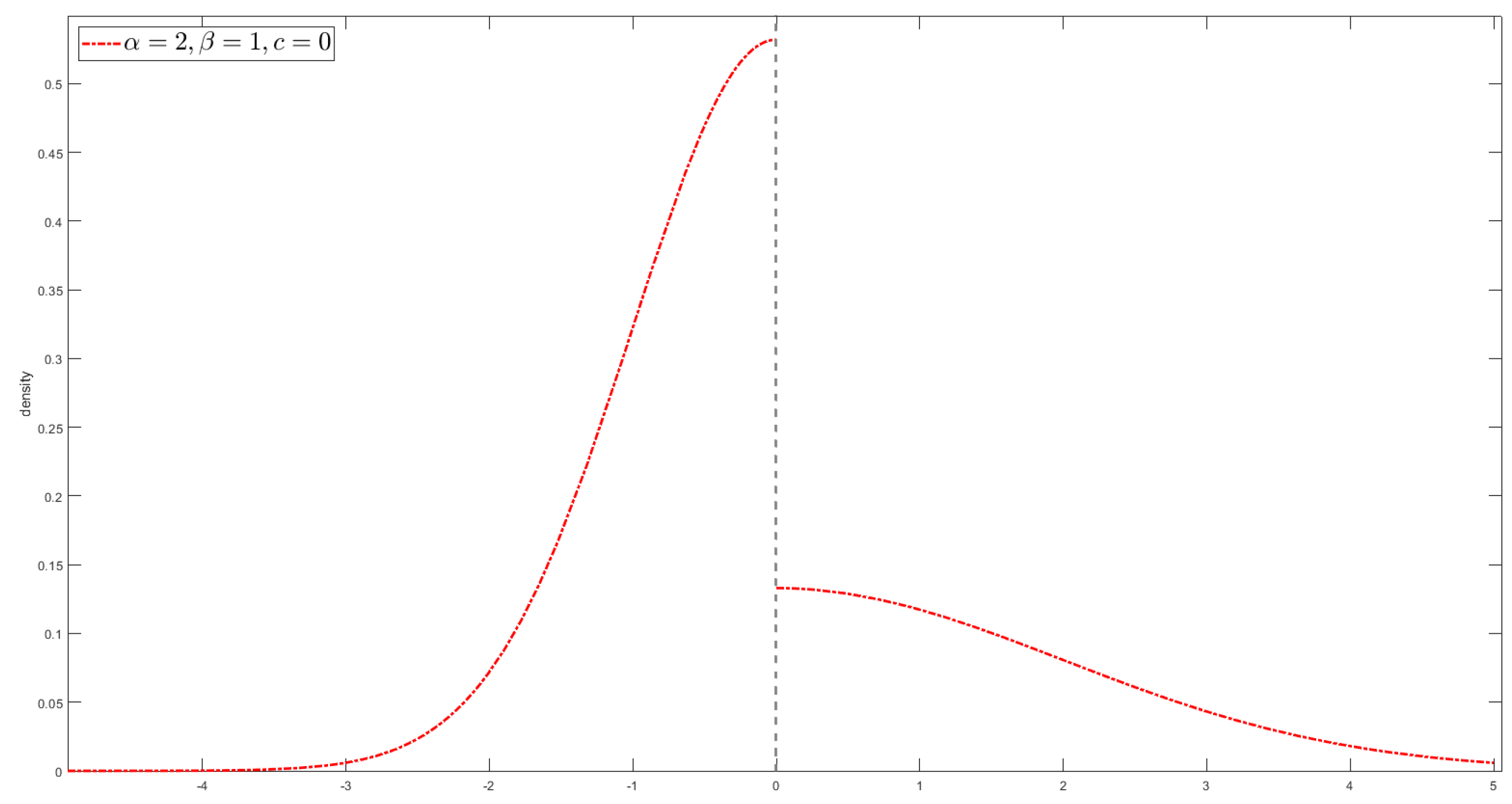
The density function of is given as follows:
and .
The above density function of the Chen–Epstein–Zhang distribution degenerates into the density function of the normal distribution only when .
Remark 2.
The assumptions and results of Theorem 11 are slightly different from those in the publication of Chen, Epstein and Zhang (2023). The frameworks and assumptions in the publication are slightly more complicated due to the consideration of the bandit problem and the construction of the optimal strategies in the Bayesian framework.
The following figure shows the curves of the density function of the Chen–Epstein–Zhang distribution.
The curve of the density function for is shown as follows (Figure 3).
The curve of the density function for is shown as follows (Figure 4).
When comparing the curves of classical normal distribution with the minimum–maximum probability density functions, one can clearly see that the minimum–maximum probability density functions are no longer continuous.
5. Differences between Classical CLT and Nonlinear CLT
For convenience, we used C-CLT to denote the classical CLT, NE-CLT to denote the nonlinear Peng’s CLT on the nonlinear expectations given by Peng, and NP-CLT to denote the nonlinear Chen–Epstein CLT under a set of probability measures given by Chen and Epstein as well as Zhang.
5.1. Frameworks
- C-CLT: The classical CLT is mainly considered on a probability space with a single probability measure . And is a sequence of random variables defined on . The distribution of each is fixed under the probability measure .
- NE-CLT: The NE-CLT is considered on the sublinear expectation space , and the random variables sequence is defined on . One can use the sublinear expectation to describe the distribution uncertainty of . When becomes a linear expectation, the nonlinear CLT degenerates into a classical one.
- NP-CLT: The NP-CLT is considered under a set of probability measures on , and the random variables sequence is defined on . One can use to describe the distribution uncertainty of . When equals the singlton , the nonlinear CLT degenerates into a classical one.
5.2. Assumptions
5.2.1. Independence
- C-CLT: Usually, are independent or is a sequence of martingale differences.
- NE-CLT: Peng provided the concept of independence on sublinear expectation space. That is, are independent on , if
- NP-CLT: When the CLT is considered on , there is no concept of independence. However, one should assume that and satisfy a property similar to independence, which can be described as followsIn fact, this holds naturally when is rectangular; see Lemma 2.2 from [40].
5.2.2. Mean and Variance
- C-CLT: Usually are identically distributed; notably, have the same mean and variance.
- NE-CLT: Peng defined the upper and lower means as followswhen , he stated that has no mean uncertainty, and defined the upper and lower variances as follows:
- NP-CLT: There are two main assumptions for the conditional means and variances of . Since there is no independence here, and the conditional means and variances of , given the information , will vary for different measures in , Chen and co-authors focused on the conditional means and variances of .
5.3. Results
5.3.1. Expression Form
- C-CLT: One usually investigates the limit behavior ofwhich is the standardization of .One haswhich has many equivalent expressions:
- NE-CLT: Usually, has no mean uncertainty, and the limit behavior of is investigated. Peng also introduced the corresponding notion of convergence in distribution in sublinear expectation space: we say that converges in distribution to G-normal distribution , if
- NP-CLT: Considering CLT with variance uncertainty, Chen and co-authors similarly investigated the limiting behavior of , assuming that has a common conditional mean of 0.Considering CLT with mean uncertainty, they investigated the limiting behavior ofThe second part is the standardization, which is similar in form to the classical CLT. Since they wanted to consider the mean uncertainty, and the standardization in the second part does not actually reflect the mean uncertainty, they added a sample mean to reflect the mean uncertainty.On the other hand, they investigated the limit behavior of the upper (or lower) expectation of the statistics for given test function, that is:Since, for a set of measures , the upper expectation or probability, that is or resp., do not have the additivity property, the above limit behavior is not equivalent to the problems (but contains them)
5.3.2. Limit Distribution
- C-CLT: The normal distribution is mostly used to describe the limit distribution.
- NE-CLT: Peng introduced the notion of G-normal distribution to characterize the limit distribution. When , it degenerated to the classical normal distribution.
- NP-CLT:
- (1)
- For the CLT with mean uncertainty, Chen and Epstein use the g-expectation or , which corresponds to the solution of BSDE (9) or (10), to describe the limit distribution. We know that the BSDE usually does not have an explicit solution, i.e., it does not have an explicit expression like the density of normal distribution. However, for some classes of symmetric test functions , Chen and coauthors found the explicit density to describe the limit distribution.
- (2)
- For the CLT with variance uncertainty, similar to the NE-CLT, one can still use the G-normal distribution to describe the limit distribution. It is also known that the G-normal distribution usually does not have an explicit expression like the density of the normal distribution. Therefore, similar to CLT with mean uncertainty, Chen and coauthors tried to find some class of functions that provides an explicit expression for the limit distribution. Then, they considered two classes of functions, and , given by (18) and (19), which are two kinds of “S-Shaped” function. For these test functions, they found the explicit expression for the density function of the limit distribution.
5.4. Proofs
5.4.1. Methods to Prove C-CLT
There are four common methods of proving the CLT:
- Method of characteristic functions;
- Method of moments;
- Stein’s method;
- The Lindeberg exchange method.
5.4.2. Methods to Prove NE-CLT
Peng first established the connection between G-normal distribution and the following nonlinear parabolic PDE, which he called G-heat equation:
He found that , where is the G-normal distribution.
Then, he represented the difference between and in terms of , and split it into n terms:
Finally, he applied the Taylor expansion and the G-heat equation to prove that the above sums converge to 0.
5.4.3. Methods to Prove NP-CLT
The idea of the proof is similar to the idea of the Lindeberg exchange method, as well as Peng’s method. It can be described in the following steps:
- Step 1: Guess the form of the limiting distribution, for example, the solution of BSDE or the G-Normal distribution. Use it to construct a family of basic functions , such thatwhere is the g-expectation corresponding to the BSDE (9).The key to constructing the function is to ensure that and equals the limit distribution.Note: In fact, the above definition is not rigorous; this is just to make it easier to understand. In the formal proof, the actual definition of differs slightly from the above definition to facilitate the proof of properties such as the smoothness and boundedness of . For example, the terminal time should not be 1 but for a sufficiently small h, and the generators of the g-expectation should be modified. See (6.3) in [40] and (A.3) in [39].
- Step 3: We use the function to connect the left- and right-hand sides of the equation in the limit theorem. Therefore, to prove the CLT, it suffices to prove thatSimilar to Lindeberg’s exchange method, as well as Peng’s method, we can divide the above differences into n parts, e.g., for CLT with variance uncertainty, we have the following:where .For the CLT with mean uncertianty, the corresponding is defined as follows
- Step 4: Using Taylor’s expansion for at , prove that the sum of the residuals converges to 0; that is,Further, using the dynamic consistency of under , one can prove thatThis leads to relation .On the other hand, using the dynamic consistency of , one has, for exampleThen, combining this with Taylor’s expansion, one can prove that .
6. Conclusions
Based on the axiomatic definition of probability theory, modern probability theory has made a number of achievements. After Kolmogorov, such scientists as the French mathematician Lévy, the Soviet mathematicians Khinchin and Prokhorov, the American mathematician Doob, the Japanese mathematician Itô, and many others made great contributions to the development of probability theory. The CLTs for random variables laid the foundation for the creation and development of stochastic analysis. This paper first provides a brief overview of the classical CLT and CLT for martingales, and then presents recent advances in CLT in the framework of nonlinear expectations. In particular, recent significant results on nonlinear CLT from the Chinese school of nonlinear expectations, including Peng, Chen, and Zhang, as well as their co-authors, are highlighted.
Among the future directions of research on nonlinear CPT, two important questions should be emphasized:
- How should the nonlinear CLT be interpreted in the case of multidimensional or high-dimensional situations?
- The convergence rate in the classical CLT has been studied quite well and has been successfully used in many applications. However, the rate of convergence in the nonlinear central limit theorem is much less investigated. How should it be treated?
The above directions are also relevant due to the active work on the mathematical justification of models and methods used in machine learning, where we often have to deal with data analysis under uncertainty.
Funding
This research received no external funding.
Acknowledgments
The research was conducted within the framework of the HSE University Basic Research Programs and within the program of the Moscow Center for Fundamental and Applied Mathematics, Lomonosov Moscow State University. The author thanks the Editor for his support and the Reviewers for their appropriate comments which have improved the quality of this paper.
Conflicts of Interest
The author declares no conflicts of interest.
References
- Rootzén, H. On the Functional Central Limit Theorem for Martingales. Z. Wahrscheinlichkeitstheorie Verw. Geb. 1977, 38, 199–210. [Google Scholar] [CrossRef]
- Hall, P.; Heyde, C.C. Martingale Limit Theory and Its Application; Academic Press: New York, NY, USA, 1980. [Google Scholar]
- Adams, W.J. The Life and Times of the Central Limit Theorem, 2nd ed. In History of Mathematics, Volume 35; American Mathematical Society: Providence, RI, USA, 2009. [Google Scholar]
- Fischer, H. A History of the Central Limit Theorem, From Classical to Modern Probability Theory; Springer: Berlin, Germany, 2011. [Google Scholar]
- Petrov, V.V. Limit Theorems of Probability Theory; Oxford Science Publications: Oxford, UK, 1995. [Google Scholar]
- Götze, F.; Naumov, A.A.; Ulyanov, V.V. Asymptotic analysis of symmetric functions. J. Theor. Probab. 2017, 30, 876–897. [Google Scholar] [CrossRef]
- Shevtsova, I.G. On absolute constants in inequalities of Berry-Esseen type. Dokl. Math. 2014, 89, 378–381. [Google Scholar] [CrossRef]
- Fujikoshi, F.; Ulyanov, V.V. Non-Asymptotic Analysis of Approximations for Multivariate Statistics; SpringerBriefs in Statistics; Springer: Singapore, 2020. [Google Scholar]
- Dedecker, J.; Merlevède, F.; Rio, E. Rates of convergence in the central limit theorem for martingales in the non-stationary setting. Ann. Inst. H. Poincaré Probab. Statist. 2022, 58, 945–966. [Google Scholar] [CrossRef]
- Bhattacharya, R.N.; Ranga Rao, R. Normal Approximation and Asymptotic Expansions; Wiley: New York, NY, USA, 1976. [Google Scholar]
- Sazonov, V.V. Normal Approximation—Some Recent Advances; Springer: Berlin, Germany, 1981. [Google Scholar]
- Bentkus, V.; Götze, F. Optimal rates of convergence in the CLT for quadratic forms. Ann. Probab. 1996, 24, 466–490. [Google Scholar] [CrossRef]
- Götze, F.; Zaitsev, A.Y. Explicit rates of approximation in the CLT for quadratic forms. Ann. Probab. 2014, 42, 354–397. [Google Scholar] [CrossRef]
- Prokhorov, Y.V.; Ulyanov, V.V. Some Approximation Problems in Statistics and Probability. In Limit Theorems in Probability, Statistics and Number Theory. Springer Proceedings in Mathematics and Statistics; Eichelsbacher, P., Elsner, G., Kösters, H., Löwe, M., Merkl, F., Rolles, S., Eds.; Springer: Berlin, Germany, 2013; Volume 42, pp. 235–249. [Google Scholar]
- Chen, Z.; Yan, X.; Zhang, G. Strategic two-sample test via the two-armed bandit process. J. R. Stat. Soc. Ser. B Stat. Methodol. 2023, 85, 1271–1298. [Google Scholar] [CrossRef]
- Peng, S.; Yao, J.; Yang, S. Improving Value-at-Risk prediction under model uncertainty. J. Financ. Econom. 2023, 21, 228–259. [Google Scholar] [CrossRef]
- Hölzermann, J. Pricing interest rate derivatives under volatility uncertainty. Ann. Oper. Res. bf 2024, 336, 153–182. [Google Scholar] [CrossRef]
- Ji, X.; Peng, S.; Jang, S. Imbalanced binary classification under distribution uncertainty. Inf. Sci. 2023, 621, 156–171. [Google Scholar] [CrossRef]
- de Moivre, A. The Doctrine of Chances, 2nd ed.; Woodfall: London, UK, 1738. [Google Scholar]
- Gauss, C.F. Theoria Motus Corporum Coelestium; Perthes & Besser: Hamburg, Germany, 1809. [Google Scholar]
- Laplace, P.S. Mémoire sur la probabilités. Mémoires de l’Académie Royale des Sciences de Paris Année 1781, 1778, 227–332. [Google Scholar]
- Lyapunov, A.M. Sur une proposition de la théorie des probabilités. Bulletin de l’Académie Impériale des Sciences de St.-Pétersbourg 1900, 13, 359–386. [Google Scholar]
- Lyapunov, A.M. Nouvelle Forme du Théorème sur la Limite de Probabilité; Mémoires de l’Académie Impériale des Sciences de St.-Pétersbourg VIIIe Série, Classe Physico-Mathématique; Imperial Academy Nauk: Russia, 1901; Volume 12, pp. 1–24. Available online: https://books.google.com/books/about/Nouvelle_forme_du_th%C3%A9or%C3%A8me_sur_la_limi.html?id=XDZinQEACAAJ (accessed on 17 July 2024).
- Lévy, P. Sur la rôle de la loi de Gauss dans la théorie des erreurs. Comptes Rendus Hebdomadaires de l’Académie des Sciences de Paris 1922, 174, 855–857. [Google Scholar]
- Lindeberg, J.W. Eine neue Herleitung des Exponentialgesetzes in der Wahrscheinlichkeitsrechnung. Math. Z. 1922, 15, 211–225. [Google Scholar] [CrossRef]
- Feller, W. Über den zentralen Grenzwertsatz der Wahrscheinlichkeitsrechnung. Math. Z. 1935, 40, 521–559. [Google Scholar] [CrossRef]
- Bernstein, S. Sur l’extension du théorème limite du calcul des probabilités aux sommes de quantités dépendantes. Math. Ann. 1926, 97, 1–59. [Google Scholar] [CrossRef]
- Lévy, P. Propriétés asymptotiques des sommes de variables aléatoires indépendantes ou enchaînées. J. Math. Appl. 1935, 14, 347–402. [Google Scholar]
- Doob, J.L. Stochastic Processes; Wiley: New York, NY, USA, 1953. [Google Scholar]
- Billingsley, P. The Lindeberg-Lévy theorem for martingales. Proc. Am. Math. Soc. 1961, 12, 788–792. [Google Scholar]
- Ibragimov, I.A. A central limit theorem for a class of dependent random variables. Theory Probab. Its Appl. 1963, 8, 83–89. [Google Scholar] [CrossRef]
- Csörgő, M. On the strong law of large numbers and the central limit theorem for martingales. Trans. Am. Math. Soc. 1968, 131, 259–275. [Google Scholar] [CrossRef]
- Brown, B.M. Martingale central limit theorems. Ann. Math. Stat. 1971, 42, 59–66. [Google Scholar] [CrossRef]
- McLeish, D.L. Dependent central limit theorems and invariance principles. Ann. Probab. 1974, 2, 620–628. [Google Scholar] [CrossRef]
- Hall, P. Martingale invariance principles. Ann. Probab. 1977, 5, 875–887. [Google Scholar] [CrossRef]
- Peng, S. Backward SDE and related g-expectation. In Backward Stochastic Differential Equations. Pitman Research Notes in Math. Series; El Karoui, N., Mazliak, L., Eds.; Longman: London, UK, 1997; pp. 141–159. [Google Scholar]
- Peng, S. Nonlinear Expectations and Stochastic Calculus under Uncertainty: With Robust CLT and G-Brownian Motion; Springer: Berlin, Germany, 2019; Volume 95. [Google Scholar]
- Peng, S. A new central limit theorem under sublinear expectations. arXiv 2008, arXiv:0803.2656. [Google Scholar]
- Chen, Z.; Epstein, L.G.; Zhang, G. A central limit theorem, loss aversion and multi-armed bandits. J. Econ. Theory 2023, 209, 105645. [Google Scholar] [CrossRef]
- Chen, Z.; Epstein, L.G. A central limit theorem for sets of probability measures. Stoch. Process. Their Appl. 2022, 152, 424–451. [Google Scholar] [CrossRef]
- Chen, Z.; Liu, S.; Qian, Z.; Xu, X. Explicit solutions for a class of nonlinear BSDEs and their nodal sets. Probab. Uncertain. Quant. Risk 2022, 7, 283–300. [Google Scholar] [CrossRef]
Figure 1.
Plots of for and and .
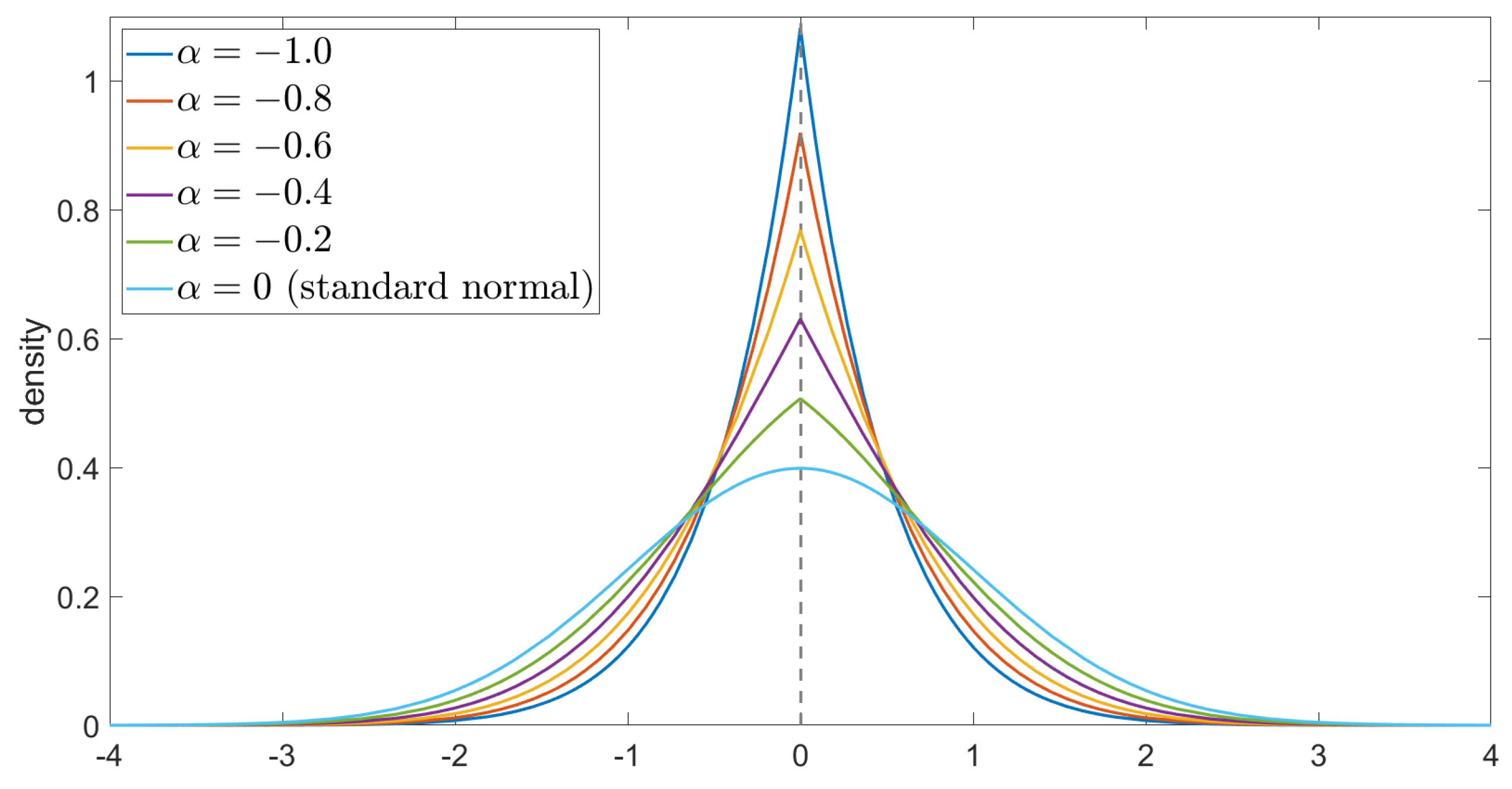
Figure 2.
Plots of for and and .

Figure 3.
Plot of for .
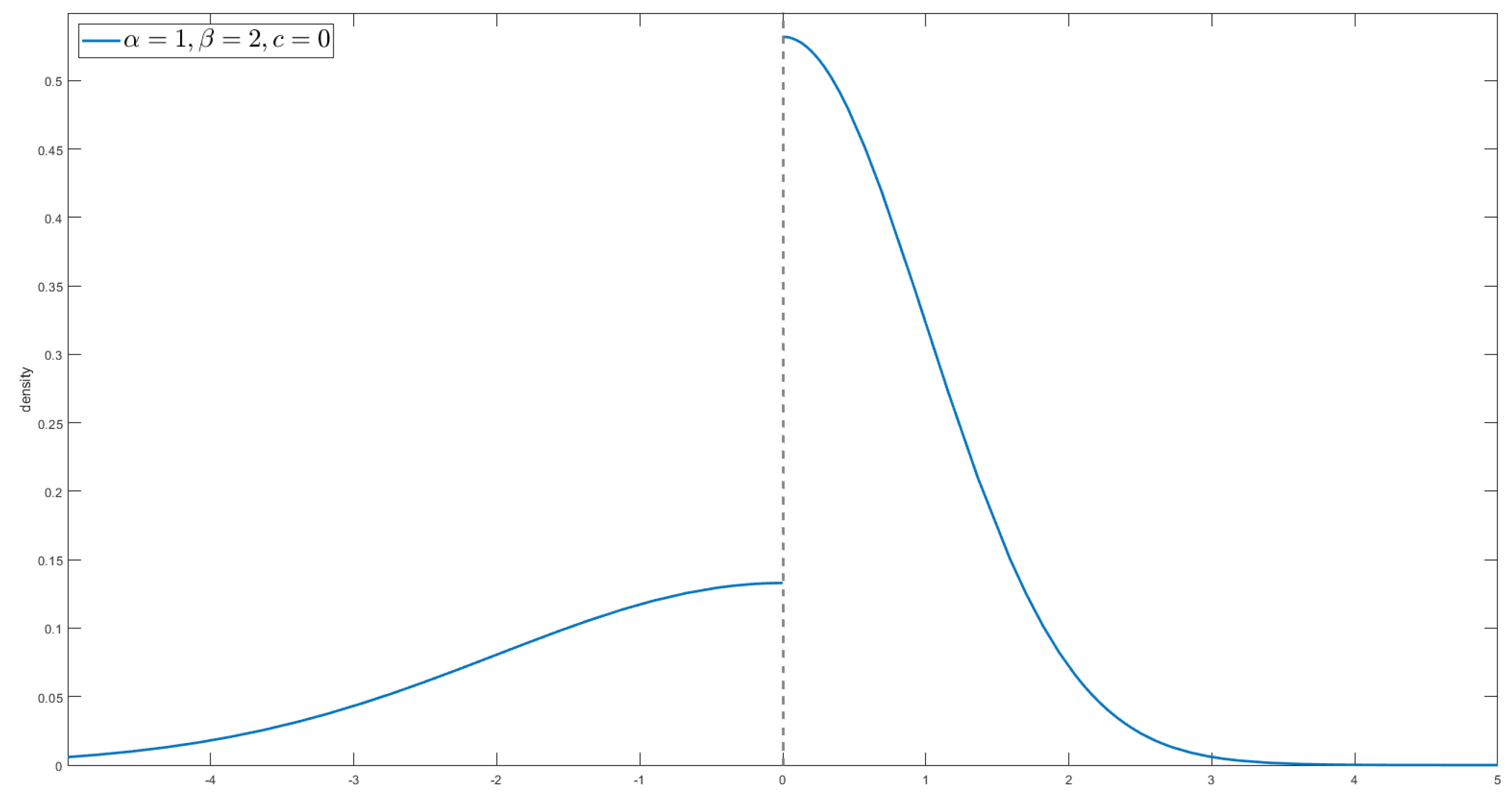
Figure 4.
Plot of for .
Disclaimer/Publisher’s Note: The statements, opinions and data contained in all publications are solely those of the individual author(s) and contributor(s) and not of MDPI and/or the editor(s). MDPI and/or the editor(s) disclaim responsibility for any injury to people or property resulting from any ideas, methods, instructions or products referred to in the content. |
© 2024 by the author. Licensee MDPI, Basel, Switzerland. This article is an open access article distributed under the terms and conditions of the Creative Commons Attribution (CC BY) license (https://creativecommons.org/licenses/by/4.0/).
Share and Cite
MDPI and ACS Style
Ulyanov, V.V. From Classical to Modern Nonlinear Central Limit Theorems. Mathematics 2024, 12, 2276. https://doi.org/10.3390/math12142276
AMA Style
Ulyanov VV. From Classical to Modern Nonlinear Central Limit Theorems. Mathematics. 2024; 12(14):2276. https://doi.org/10.3390/math12142276
Chicago/Turabian StyleUlyanov, Vladimir V. 2024. "From Classical to Modern Nonlinear Central Limit Theorems" Mathematics 12, no. 14: 2276. https://doi.org/10.3390/math12142276
Note that from the first issue of 2016, this journal uses article numbers instead of page numbers. See further details here.