Abstract
Accurate prediction of agricultural product prices is instrumental in providing rational guidance for agricultural production planning and the development of the agricultural industry. By constructing an end-to-end agricultural product price prediction model, incorporating a segmented Bézier curve fitting algorithm and Long Short-Term Memory (LSTM) network, this study selects corn futures prices listed on the Dalian Commodity Exchange as the research subject to predict and validate their price trends. Firstly, corn futures prices are fitted using segmented Bézier curves. Subsequently, the fitted price sequence is employed as a feature and input into an LSTM network for training to obtain a price prediction model. Finally, the prediction results of the Bézier curve-based LSTM model are compared and analyzed with traditional LSTM, ARIMA (Autoregressive Integrated Moving Average Model), VMD-LSTM, and SVR (Support Vector Regression) models. The research findings indicate that the proposed Bézier curve-based LSTM model demonstrates significant predictive advantages in corn futures price prediction. Through comparison with traditional models, the effectiveness of this model is affirmed. Consequently, the Bézier curve-based LSTM model proposed in this paper can serve as a crucial reference for agricultural product price prediction, providing effective guidance for agricultural production planning and industry development.
MSC:
03-08; 03-11; 65J08; 68U99; 97N80; 97P40
1. Introduction
China is an agricultural giant, and the development of agriculture is of paramount importance. Agricultural products are crucial foundations for the rural economy in China, and accurately predicting their prices is essential for ensuring stable income for farmers and meeting the daily needs of society [1,2,3]. By effectively predicting agricultural product prices, we can analyze the characteristics and patterns of price fluctuations, thereby reducing the impact of unforeseen factors on the economy. Additionally, by establishing effective models for predicting agricultural product prices, we can more accurately analyze price trends. Accurately predicting agricultural product prices not only provides rational recommendations for government decision-making but also offers effective support for determining target prices for agricultural products. This can effectively guide the development of the agricultural product industry, thereby promoting the prosperity and healthy development of the agricultural economy [4,5].
Traditional prediction models for agricultural product prices primarily encompass time series analysis, regression analysis, and an array of associated linear and nonlinear modeling techniques. Ren Weijie and Li Baisong [6] proposed a new method called the Hilbert–Schmidt independence criterion Lasso Granger causality, which is used to reveal nonlinear causal relationships between multivariate time series. The results show that the proposed method can effectively analyze the nonlinear causal relationships between multivariate time series and can simultaneously conduct causal analysis of multiple input variables for output variables, which is suitable for addressing high-dimensional problems. Weng Yucheng [7] and others tested Autoregressive Integrated Moving Average (ARIMA) models, backpropagation (BP) neural network methods, and recursive neural network (RNN) methods to predict the short-term (several days) and long-term (several weeks or months) prices of agricultural products (cucumbers, tomatoes, and eggplants). They found that the ARIMA model requires continuous and periodic data, so it is apt for handling small-scale periodic datasets. It excels with average monthly data but struggles with daily data. Conversely, neural network approaches, such as backpropagation networks and Recurrent Neural Networks (RNNs), are adept at forecasting daily, weekly, and monthly price volatility trends effectively. Varun [8] and others laid a practical foundation for future predictions by studying the impact of foreign exchange rates on agricultural product price changes using multivariate regression techniques and data mining. Brandt and Bessler [9] used 24 quarters of U.S. pork as the research object and employed seven forecasting methods for verification and performance evaluation, deriving the value of the forecasting methods.
In order to address various issues regarding prediction accuracy and effectiveness, experts and scholars have proposed various intelligent forecasting methods. Purohit, SK [10] introduced two additive hybrid methods (Additive-ETS-SVM, Additive-ETS-LSTM) and five multiplicative hybrid methods (Multiplicative-ETS-ANN, Multiplicative-ETS-SVM, Multiplicative-ETS-LSTM, Multiplicative-ARIMA-SVM, Multiplicative-ARIMA-LSTM) for predicting the monthly retail and wholesale prices of three commonly used vegetable crops in India (tomatoes, onions, and potatoes). They confirmed the superiority of hybrid methods in forecasting TOP prices. Raflesia [11] and others studied agricultural sales systems and applied the PSO particle algorithm to construct radial basis function neural networks for price prediction of different agricultural products. Zhao Hailei [12] first used wavelet analysis to smooth the data, then constructed a model to process the hierarchical information after signal decomposition, and finally used the ARIMA algorithm for analysis. They found that using wavelet analysis yielded better results than using the ARIMA model alone, affirming the importance of data smoothing. Liu Jindian [13] and colleagues proposed a soybean futures price prediction model based on Ensemble Empirical Mode Decomposition (EEMD) and New Attention Gating Units (NAGU). The results showed that the predictive performance of the EEMD-NAGU model was superior to other models such as LSTM, GRU, NAGU, EEMD-LSTM, EEMD-GRU, and EEMD-NGU. This model can be widely used to predict the prices of wheat, corn, gold, oil, and other time series data. Abdullah [14] and others established linear and nonlinear models to better predict coconut prices and studied the capabilities of a hybrid method combining ARIMA and NARNET (ANN) models. Experimental results showed that the proposed ARIMA-NARNET method outperformed the ARIMA model and the NARNET model in predicting coconut prices. Liu Weiping [15] and others proposed a novel method that combines Variational Mode Decomposition (VMD) and Artificial Neural Networks (ANN) into a “Decomposition and Integration” framework. This method transforms the high-volatility futures price prediction problem into predicting multi-component time series with a unique central frequency, then independently predicts all components using the ANN method, and finally integrates the prediction results of each component into the final prediction result. The results showed that both accuracy and trend accuracy were significantly better than some state-of-the-art methods, validating that the proposed VMD-ANN method can effectively predict non-stationary and nonlinear futures price sequences. Zhang [16] combined the linear prediction advantages of the ARIMA model with the nonlinear prediction features of the ANN model and found that the combined model had higher prediction accuracy. Gu Yongxian [17] and others proposed a model called Dual Input Attention Long Short-Term Memory (DIA-LSTM), which, compared to traditional models using static meteorological information from the main production areas, reduced the Mean Absolute Percentage Error (MAPE) by 2.8% to 5.5%. Moreover, its MAPE was lower than the benchmark model by 1.41% to 4.26%. Ray, S [18] and others proposed an improved hybrid ARIMA-LSTM model based on the Random Forest Lagged Selection Criterion. The results showed that the proposed model outperformed traditional statistical models, with RMSE increasing by 8–25%, MAPE increasing by 2–28%, and MASE increasing by 2–29%. Simões [19] and Sivapragasam [20] constructed SVM prediction models based on SSA for short-term random rainfall prediction, validating that the models had higher prediction effectiveness and result confidence. Paul [21] and others used machine learning algorithms such as GRNN and SVR to forecast eggplant prices in the Indian state of Odisha and tested the accuracy of different models through the Diebold–Mariano test.
The focus of this paper is the prediction model of corn futures price based on the LSTM Bezier curve. Bezier curve is a parametric polynomial curve based on the Bornstein basis function, and the shape of the curve is adjusted by the coordinates of the control points. Designers without mathematical knowledge can also complete interactive design modification work, so it is widely used in CAD design software. The greatest advantage of Bezier curves is the flexibility to change the shape of the curve by moving the control points, and because of the consistent approximation of Bornstein basis functions to polynomials (and even continuous functions), it is an excellent curve fitting tool. The Bezier curve fits the data point column as follows: First, the logarithmic data point column is parameterized (isometric parameterization, cumulative chord-length parameterization, modified sine length parameterization, etc.) so that each data point corresponds to a parameter t in the interval [0,1], and then the least square fitting method is used to obtain a fitting curve that minimizes the distance between each data point and the curve, thus revealing the intrinsic basic trend of the data point column.
Krishna [22] proposed a convolutional recurrent neural network (ConvRNN) kernel based on wavelet to improve the time–frequency localization of non-stationary signals, applied Bezier–Bernstein polynomial functions to model NSS, and used inflection points for signal segmentation. From the obtained fragments, statistical time–frequency features are extracted and fed to the ConvRNN for better time–frequency localization. Bai [23] proposed an improved path planning algorithm based on deep reinforcement learning to find a class of AMR optimization paths, in which Bessel curve theory was used to smooth the planned paths.
As a special recurrent neural network structure, Long Short-Term Memory (LSTM) is mainly used to improve and solve the long-term dependence problem encountered in traditional RNN. LSTM is able to control and transmit information using a unique gating mechanism to better capture long-term dependencies.
Huang Y [24] proposed a coal seam thickness prediction method based on VMD and LSTM methods. The VMD method is used to denoise the signal, and compared with the EMD method, the result of VMD is proved to be better. Then, LSTM is used to predict the thickness of the coal seam, and compared with other benchmark models, it is found that the prediction method proposed by him has higher accuracy, which indicates that the data denoising can help improve the prediction accuracy. Otero [25] used a multivariate empirical mode decomposition method to decompose the original time signals collected from the training set and patients with essential tremors. The decomposed data are respectively input into the LSTM model for training and prediction, and then all prediction results are added together to form the final prediction result. Finally, the trained LSTM model is obtained. Then, the remaining raw samples are used to test the model. The experimental results show that the proposed method is superior to all other benchmark methods in all cases.
Finally, As an important agricultural product, corn has the characteristics of high supply and demand and high price fluctuation. Accurate analysis of corn prices and prediction of future corn prices based on this can effectively guarantee the stable development of corn planting, breeding, and corn processing industries and also help the government to timely regulate corn prices and reduce possible crises [26,27,28]. Therefore, this study will focus on the fluctuation of corn prices. With the benchmark LSTM and ARIMA models, a corn futures price prediction model based on the Bezier curve is proposed to effectively analyze and forecast the daily futures price of corn, providing a scientific basis for the government and related enterprises to formulate relevant policies.
2. Methods
2.1. Bézier Curve
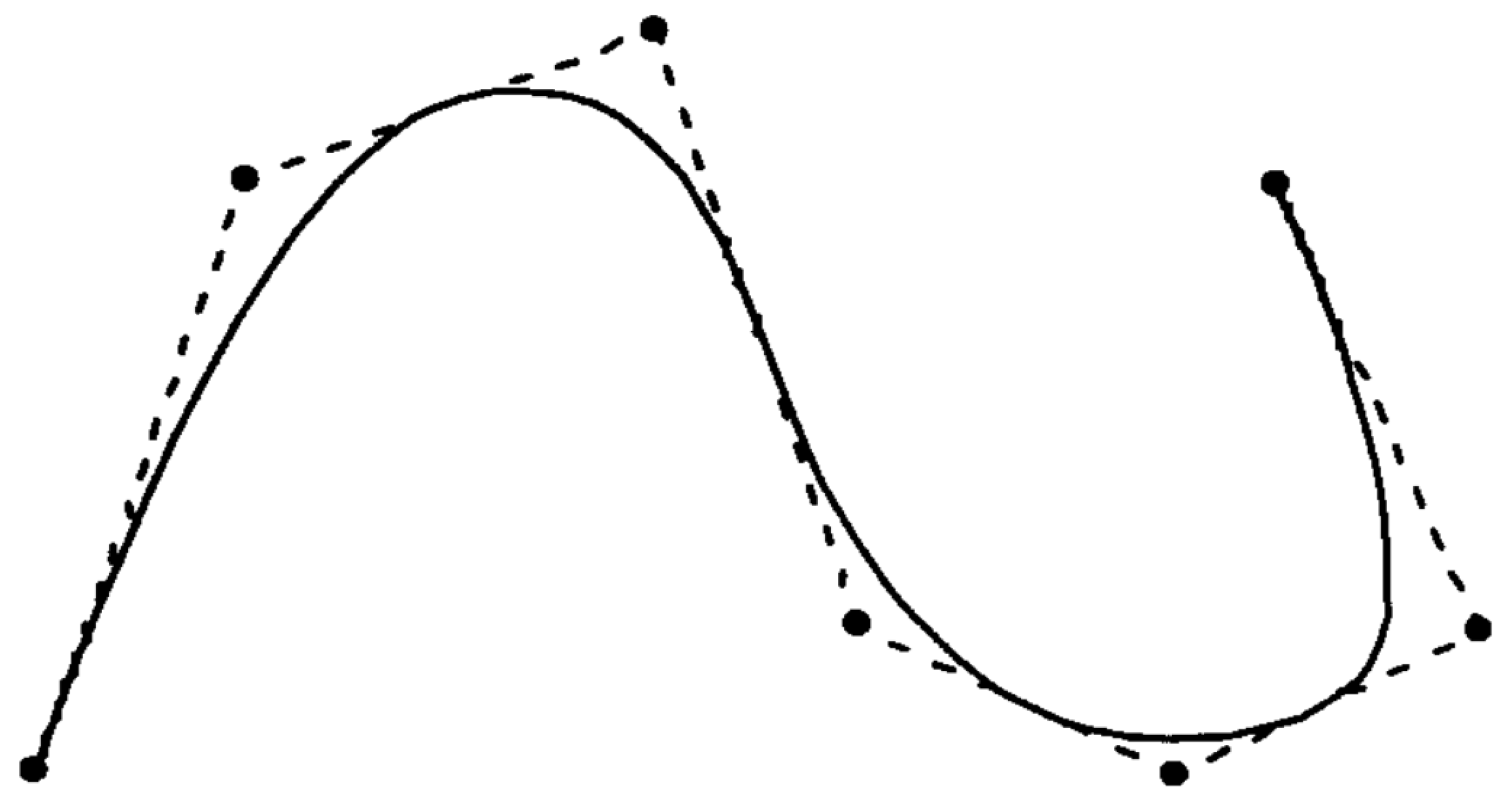
The Bézier curve [29,30] is a parametric polynomial curve based on Bernstein basis functions. Due to the uniform approximation property of Bernstein polynomials for continuous functions, the Bézier curve has become an excellent curve fitting tool. The shape of a Bézier curve can be adjusted by changing the coordinates of control points, and a single Bézier curve is continuously differentiable at every parameter point [31,32]. At the start and end points, the Bézier curve is tangent to the first and last two edges of the characteristic polygon, respectively, and the entire curve lies within the convex hull of the characteristic polygon, with its overall trend closely following that of the characteristic polygon (see Figure 1).

Figure 1.
Bézier curve fitting diagram.
In this article, Bézier curves are used to fit corn futures prices based on the least squares criterion, defined as follows:
Definition 1.
Given points in a plane or space, where is called a control point, the n-sided polygonal line formed by connecting adjacent points in sequence is called the control polygon [33]. The corresponding nth-degree Bézier curve is defined as follows:
where is the Bernstein basis function. Its polynomial representation is as follows:
When , it is a cubic Bezier curve with four control points , as follows:
As long as four control vertices of the characteristic polygon are given, and a cubic Bézier curve can be constructed by using the above formula, the matrix expression is as follows:
2.2. The Basic Principle of Long Short-Term Memory (LSTM) Networks
2.2.1. LSTM Process
Long Short-Term Memory (LSTM) neural networks [34,35,36] have four structures: the forget gate, the input gate, the output gate, and the memory cell. These components control the LSTM process by utilizing the forget gate and the input gate. The LSTM process is as follows (see Figure 2).
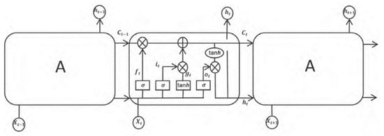
Figure 2.
LSTM process flow diagram.
The arrows in the diagram represent the direction of data flow, indicating the input from the previous node to the node pointed to by the arrow. LSTM processes input information through three control gates, each gate consisting of a sigmoid activation function and a multiplication structure [37]. The sigmoid activation function in the gate is defined by Equations (5) and (6), while the hyperbolic tangent function (tanh) is defined by Equations (7) and (8).
where
: The unit state passed from the previous time step;
: The new information value read in at the current time step, thereby allowing this module to generate new memories;
: The output value of the previous hidden neuron module;
: The unit state belonging to the information output at the current time step, passed to the next time step;
: The new output at the current time step.
2.2.2. LSTM Propagation Computation
- (1)
- The process of forward propagation computation in LSTM begins with the forget gate. The process of forward propagation computation in LSTM begins with the forget gate. Finally, the data of the cell unit and the input data are input to the output gate.
The forget gate combines the output data of the previous output gate with the new input data to determine the degree of data forgetting in the cell unit. After and are activated by activation function, is obtained. represents the degree of retention of the previous hidden neuron state, the activation function is sigma, and the expression is as follows:
where
: The weights of the previous hidden neuron module input to the forget gate;
: The weights of the input layer information flowing into the forget gate;
: The bias parameters when computing the forget gate.
The input gate determines how much information will be received, decides what new information will be generated, and how much of the new information will be used. The calculation process is as follows:
After passing through the input gate, its output is .
The update of the memory cell state involves multiplying the output of the forget gate with the previous time step’s cell state and combining it with the output of the input gate to obtain the new cell state . is formed by combining a portion of the information from the previous time step with the newly generated information [38,39]. The expression for is as follows:
Finally, after passing through the output gate, is calculated by combining the current information with the short-term memory. is then calculated by combining the long-term memory with . is formed by combining the output value of the previous hidden neuron module with the current input value and activating it with the sigmoid function. The calculation process is as follows:
After passing through the LSTM model, the final output is as follows:
- (2)
- LSTM backpropagation requires updating the weights and relevant biases in the model after forward propagation computation. This can be achieved by propagating errors backward to the preceding layer for calculation.
2.3. Differential Autoregressive Moving Average
ARIMA stands for Autoregressive Integrated Moving Average, which is a widely used and traditional time series analysis model. It primarily analyzes time series data by modeling the past values of a stochastic variable and random disturbances [40,41].
- (1)
- Autoregressive Model
The autoregressive model refers to the relationship between the current value and past values, utilizing past data of the variable to predict its own future values. The premise for autoregressive model prediction is that the data must be stationary. The formula for a p-order autoregressive model can be expressed as follows:
: Current value of the variable;
: Constant term;
: Order;
: Autocorrelation coefficient;
: Residuals.
- (2)
- Moving Average Model
The moving average model expresses linear relationships using past values of residuals to observe fluctuations. In prediction, the main role of the moving average method is to eliminate the random volatility in the forecasting process. represents the calculation of q-th order moving averages, expressed as follows:
- (3)
- Autoregressive Moving Average Model ARMA
ARMA is the combination of the AR model and the MA model, where represents the order of autocorrelation in the autoregressive component, and represents the maximum order of autocorrelation in the moving average component. The model expression is as follows:
The ARIMA model [42,43] is an extension of ARMA . Before determining the parameters and , the data need to undergo tests for stationarity and white noise. If the data are non-stationary, differencing is performed. After differencing d times, a stationary series is obtained, and then a model can be established.
2.4. Support Vector Machine Regression Principle
Support Vector Machine [44] (SVM) is a binary classification model that maps input vectors into a high-dimensional space and finds a hyperplane in this space to separate vectors of different classes. Support Vector Regression [45,46] (SVR) is a method that utilizes SVM for regression analysis. It seeks to find a linear or nonlinear hyperplane in high-dimensional space that minimizes the difference between actual and predicted values to achieve prediction. First, the input space is mapped into a high-dimensional space, and then the optimal separating hyperplane is found in this space while maximizing the margin distance within a certain error range. The advantages of the SVR model include suitable generalization ability, high-dimensional performance, nonlinear capabilities, and applicability to various data types and scenarios [47].
The training sample of the SVR model is , and its final loss is 0 if the model is exactly the same as . The deviation of maximum between and is set in the SVR model, and when the difference between and is greater than , then the loss needs to be calculated, and if the distance is less than , there is no need to calculate the loss [48]. It is equivalent to establishing a wide interval band centered on . If the sample data fall between the interval bands, the prediction is accurate, as shown in Figure 3.
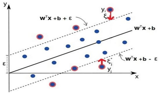
Figure 3.
Support Vector Machine regression display diagram.
In Support Vector Machine (SVM) regression, there are two parameters involved: and . represents the loss function, which affects the accuracy and training speed of the entire model and is an important indicator for measuring the predictive accuracy of the SVR model. Parameter is the penalty factor, aimed at balancing the model. A smaller value of indicates lower model complexity and correspondingly less penalty. Both the penalty factor and the parameter gamma of the kernel function have a significant impact on the model performance, thus requiring the selection of appropriate methods to optimize and select the two parameters for the SVR model based on specific problems.
By combining Bayesian optimization with manual adjustment, a prior distribution is first set for the range of values of and gamma. Bayesian methods are then used to update this distribution to help select the best-performing parameters. Next, different values of gamma are tried with different values of as a baseline to further adjust the model’s performance, determining the optimal combination of values for and gamma.
2.5. Variational Mode Decomposition (VMD) Principle
Variational mode decomposition [49], proposed by Konstantin Dragomiretskiy in 2014, can well suppress the mode aliasing of EMD methods (by controlling the bandwidth to avoid aliasing). VMD decomposition diverges from the EMD principle by employing an iterative search to identify the optimal parameters of a variational model, specifically the central frequency and bandwidth for each constituent element of the decomposition. This approach is characterized by a fully non-recursive model. The process aims to discover a collection of modal components along with their central frequencies, ensuring that each mode remains smooth once it has been demodulated to the baseband. Konstantin Dragomiretskiy’s experimental results show that the method is more robust for sampling and noise. The main decomposition steps of the VMD algorithm are as follows:
For each mode function , the Hilbert transform is used to calculate the corresponding analytic signal, and then its unilateral spectrum is obtained:
In Equation (18), is a Dirac delta function, is an imaginary unit, and stands for convolution operation.
For every individual mode, adjust the frequency spectrum to the “baseband” through a process of mixing it with an exponential function that is aligned with the estimated central frequency of that mode.
In Equation (19), represents the index of the central frequency. Utilizing the estimated bandwidth of the Intrinsic Mode Function (IMF), the variational constraint equation can be derived:
and serve as concise symbols for the entire collection of modes and their corresponding central frequencies. is understood as the summation over all modes.
To achieve the optimal solution, the augmented Lagrange formulation is derived by incorporating a quadratic penalty term, denoted by , and a Lagrange multiplier, represented by . The purpose of aims to guarantee the fidelity of signal reconstruction even in the presence of noise, while is introduced to uphold strict adherence to constraints throughout the solution process.
The Alternating Direction Method of Multipliers (ADMM) is employed to tackle the equation. To accomplish full signal decomposition, the central frequencies of each Intrinsic Mode Function (IMF) are segmented based on the frequency domain traits of the original signal, followed by an update to the central frequencies of the IMFs. The revised expression for the IMF is presented as follows:
The Fourier transform is applied to convert the formula from the time domain to the frequency domain. Subsequently, the integration over the non-negative frequency domain interval is performed to derive the optimal solution. Within this process, the frequency domain calculation criterion for each Intrinsic Mode Function (IMF) is expressed as follows:
The updated iteration formula of IMF center frequency is as follows:
In Equation (23), is the Wiener filter of , and is the frequency spectrum center of each IMF.
3. Empirical Research
3.1. Experimental Environment and Data
The experiments in this paper were conducted on a Windows 10 64-bit operating system, using an AMD Ryzen 7 5800H with Radeon Graphics 3.20 GHz processor and 16 GB of memory. The programming language used was Python 3.7.5, with the Matplotlib 3.0.2 plotting tool.
The data for this study were sourced from the Dalian Commodity Exchange’s corn futures market data. The empirical analysis covers the price series from 4 January 2013 to 30 December 2022, totaling 10 consecutive years of working days, with a total of 16,038 original data points. The dataset includes 12 different indicators, namely, the previous closing price, previous settlement price, opening price, highest price, lowest price, closing price, settlement price, price change ratio 1, price change ratio 2, trading volume, trading value, and open interest. Each year includes 12 different contract prices. The original dataset is formatted as shown in the Table 1 below (PCP means previous closing price, PST means previous settlement price, OP means opening price, HP means highest price, LP means lowest price, CP means closing price, SP means settlement price, PF means price fluctuations, and TV means trading volume).

Table 1.
Corn futures price data table.
- (1)
- Contract Selection: When selecting contracts, we refer to the main contract, which is the contract with the largest open interest. In cases where open interest is the same, we choose the contract with higher trading volume, and if trading volume is also the same, we select the contract with a later expiration date. To filter the main contract, we use the pandas library in Python for calculation. After filtering, we obtained a total of 2430 main contract data points.
- (2)
- Price Selection: The data source includes seven different price indicators: previous closing price, previous settlement price, opening price, highest price, lowest price, closing price, and settlement price. In our study, we choose the settlement price as the research object. The settlement price is the final delivery price of the futures contract on the expiration date or specified date, and it plays a crucial role in the futures market [50,51].
Therefore, by ensuring the selection of appropriate contracts and focusing on the settlement price as our key indicator, we ensure the effectiveness of corn price prediction. After organizing and processing the data, we obtained a total of 2430 daily price data points for corn futures, and the price trend chart is shown in Figure 4.
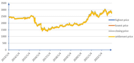
Figure 4.
Corn daily futures price series chart.
3.2. LSTM Model Construction and Prediction Analysis
In data set partitioning, most models divide the training set and the test set in a 7:3 ratio because the data volume of these data is usually large. In the process of data splitting, due to the small amount of data, in order to avoid the problem of underfitting the model due to the lack of learning of some features, the training set and the test set are divided according to the ratio of 8:2. If the ratio of 9:1 is divided, it may lead to the problem of overfitting the training set results and poor test set results, and the test set data of this division is too small to show the prediction effect over the whole year. After comparing the results of the algorithm model with these three partitioning methods, it is found that partitioning according to the ratio of 8:2 is slightly better than the other two methods, and the test set of this partitioning can cover a whole year’s data, which is more conducive to observation. Therefore, this paper divides the training set and the test set in an 8:2 ratio.
To analyze and predict the daily price dataset of corn futures, we divided the dataset into training and testing sets using an 80:20 ratio. The first 80% of the data was used as the training set, while the remaining 20% was used as the testing set. Considering the characteristics of the data and the business requirements, we used the training data of corn futures prices as input to the LSTM network and set the output layer dimension to 1. To evaluate the performance of the model, we chose Root Mean Squared Error (RMSE) as the evaluation metric and used cross-validation to continuously evaluate and optimize the parameters. We determined the following settings: 4 hidden layers, 3000 iterations, and historical time steps of 2. To improve training accuracy, we set the batch size to 480 and added a dropout layer to prevent overfitting. All layers were fully connected during training, and the sigmoid activation function was used. Based on these parameter settings, we trained the model and conducted predictive analysis on the testing set data.
For model evaluation, we chose three evaluation metrics to measure the predictive performance of the model: Mean Absolute Percentage Error (MAPE), Root Mean Squared Error (RMSE), and directional statistical indicator.
- (1)
- MAPE (Mean Absolute Percentage Error)
Mean Absolute Percentage Error (MAPE) is calculated by taking the average of the percentage errors, where each percentage error is the absolute difference between the predicted and actual values divided by the actual value. When the actual value is small, it can significantly influence the MAPE value since the denominator becomes small. This can affect the evaluation of the model. The formula for MAPE is as follows:
- (2)
- RMSE (Root Mean Squared Error)
Root Mean Squared Error (RMSE) is a measure of the average deviation between observed values and true values, calculated by taking the square root of the average of the squared differences between the observed and true values. RMSE is used to describe the dispersion of the sample, and when performing nonlinear fitting, a smaller RMSE indicates better performance. Using RMSE to define the loss function has the advantage of being smooth and differentiable, making mathematical calculations easier.
The formula for RMSE is as follows:
In the equation, represents the number of samples, denotes the predicted price value at time period , and represents the true price value corresponding to time period .
- (3)
- (Di-Rectional Statistic)
In addition, the statistical indicator is introduced on top of MAPE and RMSE to measure the directional accuracy of the model’s predictions, providing a better assessment of the model’s performance in predicting price changes. A higher value indicates better performance. can be represented as follows:
where
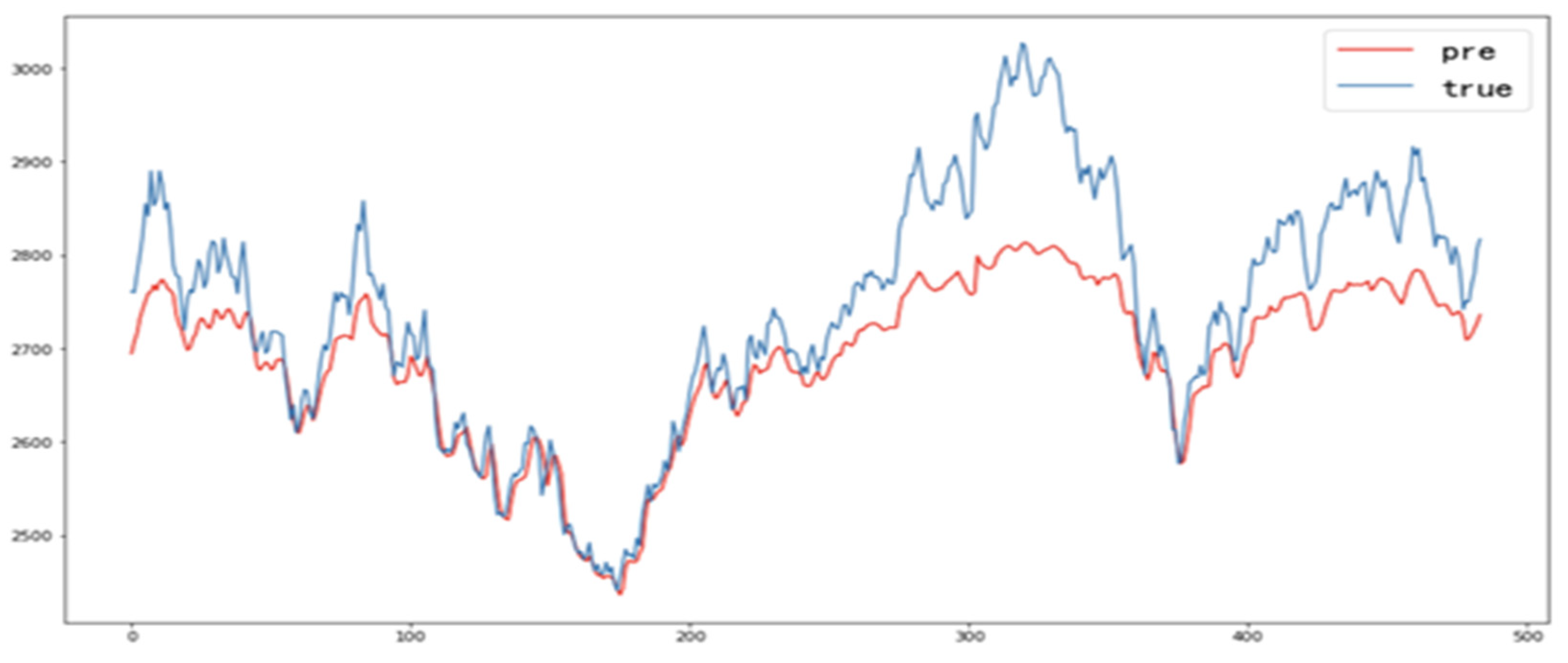
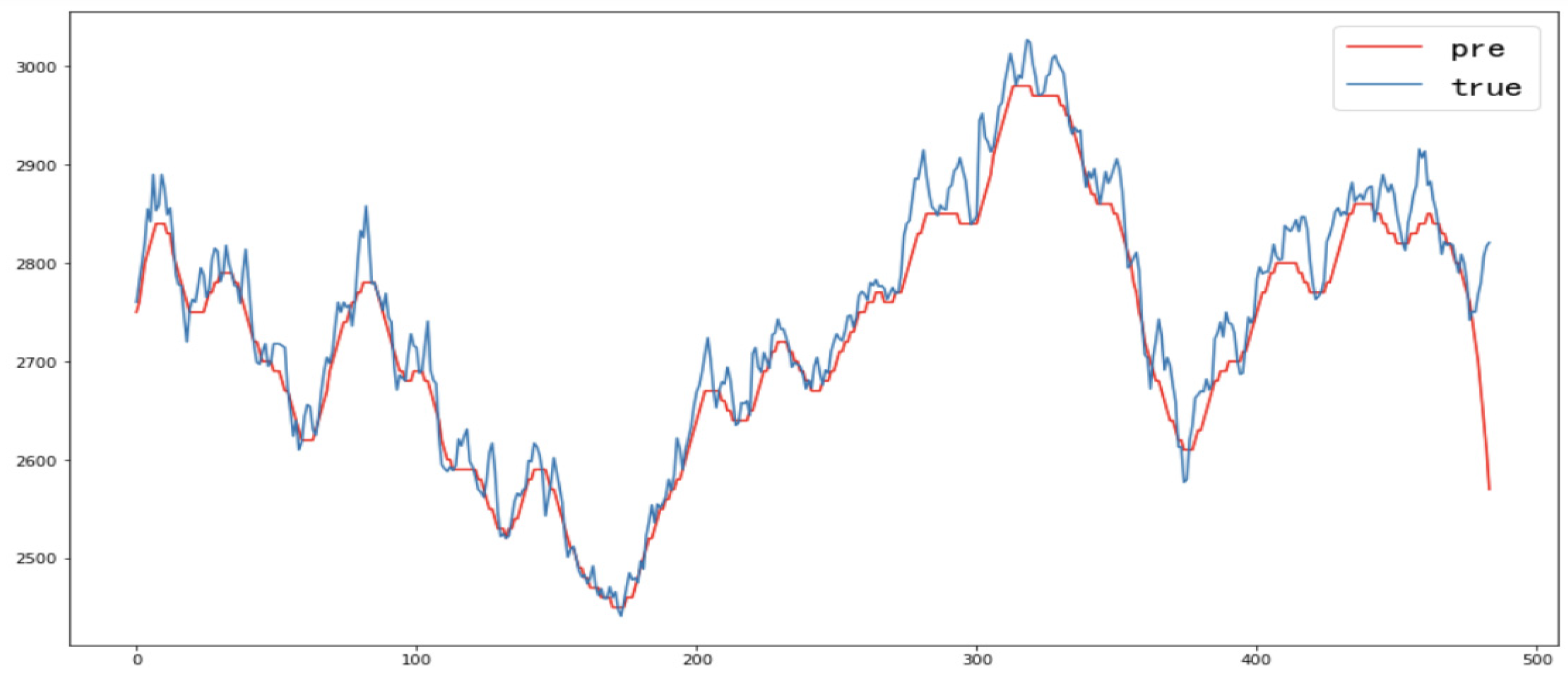
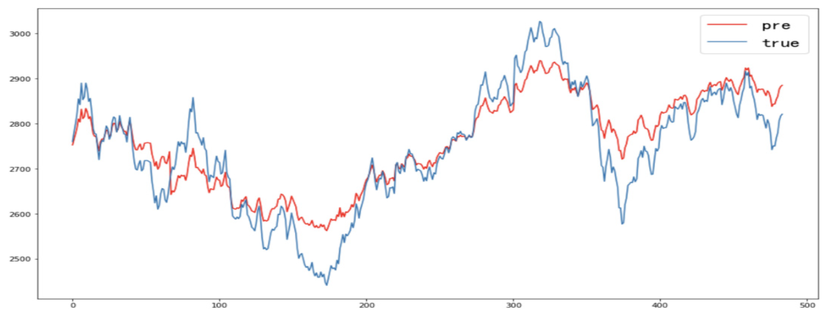
The corn futures price data set is divided into a ratio of 8:2; the first 80% is selected as the training set of the model, and the last 20% is selected as the test set. Considering the characteristics of the data and business requirements, the training set data of corn futures price are taken as the input of the LSTM network, the batch_size is set to 480, the network parameters are updated using the backpropagation algorithm, the dropout layer is applied to minimize the loss function, and sigmoid is selected as the activation function. Set the hidden layer to 4, epoch to 2000, and time step to 2. All layers will be fully connected during the training process, and the sigmoid will be selected as the activation function. Based on the above parameters and model training, the LSTM model is constructed to predict and analyze the multi-factor test set data. The LSTM model prediction results and index results are shown in Figure 5 and Table 2.
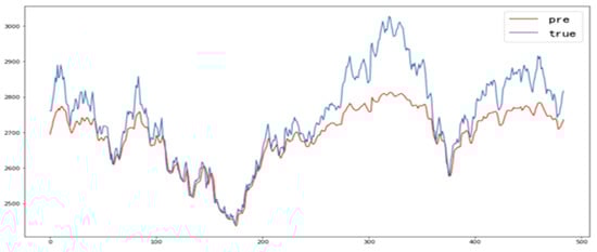
Figure 5.
LSTM model prediction results.
Table 2.
LSTM model prediction results index value.
Based on the analysis of the evaluation metrics RMSE, MAPE, and for corn settlement prices, it is observed that these metrics did not achieve satisfactory results. Particularly, the MAPE value of 1.6% is considered too high. Combining the analysis of the results with the graphs, it is concluded that using the LSTM model alone for predicting corn prices results in reasonably accurate short-term price predictions but introduces some bias in predicting long-term price trends. Although the model can roughly predict price trends and characteristics, the achieved predictive performance is not ideal.
3.3. Bezier-Based LSTM Model Construction and Prediction Analysis
Before predicting the corn price series, we first utilize Bézier curves to fit the data sequence, approximating the basic trend in the time series data. Segmented Bézier curves are defined, dividing the interval into 10 segments. According to the requirements of segmented Bézier curves, corresponding basis functions are provided, with each basis function corresponding to a control point. For example, for a segmented fifth-order Bézier curve, the basis functions for the first segment, denoted as , are as follows:
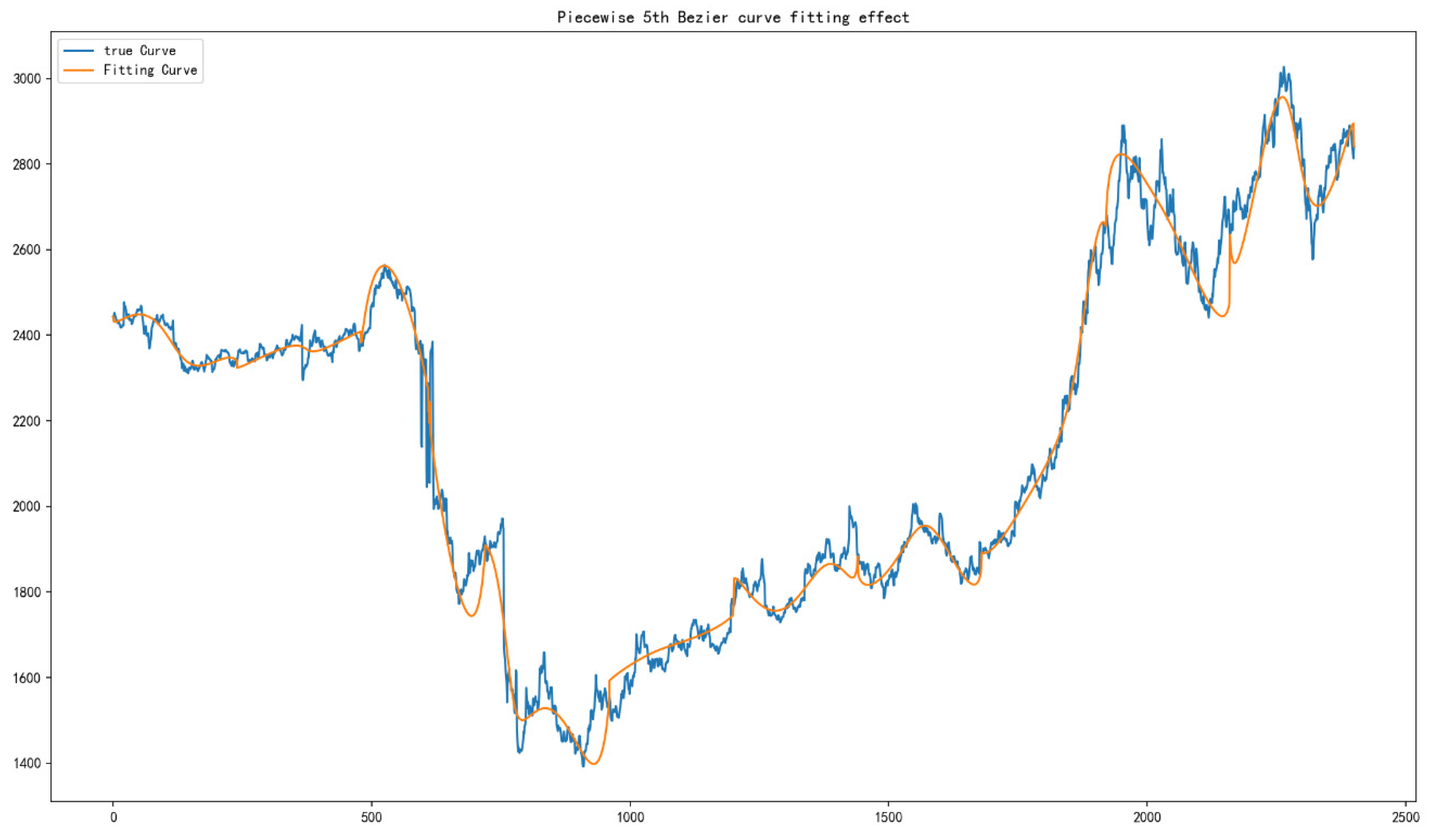
The corresponding control points are , totaling 6 points. The basis functions for other segments can be obtained through coordinate translation and symmetry. Therefore, a segmented fifth-order Bézier curve divided into 10 equal segments has 51 basis functions in total. Using the chord-length parameterization method, specific values of the parameter corresponding to each data point are obtained. Then, the specific coordinates of each control point are calculated through the least squares fitting method, resulting in the final fitted curve [52]. Through multiple experiments, it is observed that the segmented fifth-order Bézier curve provides better detail fitting without knotting phenomena occurring. The fitting effect is shown in Figure 6.
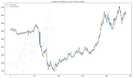
Figure 6.
Piecewise 5th Bezier curve fitting effect.
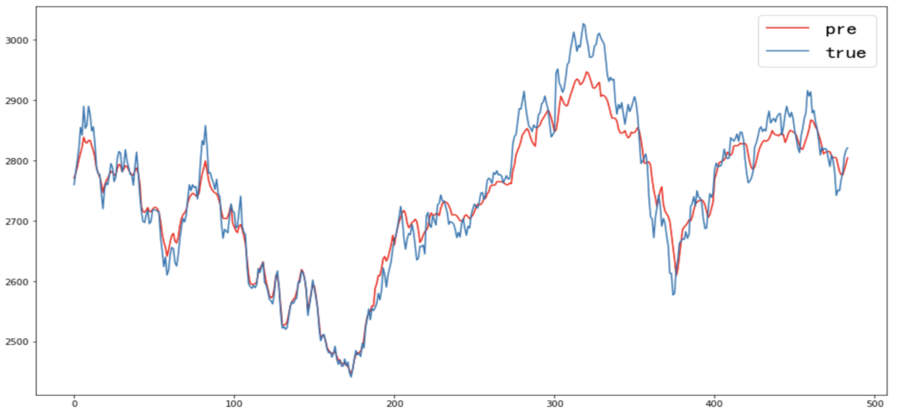
With the data generated from the Bézier curve, the corn futures price dataset is divided into a ratio of 8:2, with the first 80% for training the model and the remaining 20% as a testing set. That is, the training set data are used as the input to the LSTM network, with the output layer dimension set to 1. RMSE is chosen as the evaluation metric, and parameters are continuously evaluated and optimized using cross-validation. The settings for the hidden layer are determined as 3, with 2000 iterations and a historical time step of 2. To improve training accuracy, the batch size is set to 100, a dropout layer is added to prevent overfitting, and all layers are fully connected during training. Sigmoid is chosen as the activation function. Based on these parameter settings, the model is trained, and predictions are made on the testing set. Therefore, the predicted results of the LSTM model based on Bézier are shown in Figure 7. The index results of Bezier + LSTM model are shown in Table 3.
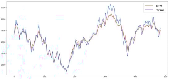
Figure 7.
Bezier + LSTM model prediction results based on Bezier.
Table 3.
Index value of prediction result of LSTM model based on Bezier fitting.
Therefore, it can be concluded that by first processing the corn settlement prices, fitting them using Bézier curves, and then entering them into LSTM for prediction, the combination of Bézier curves and LSTM models for forecasting shows significant advantages in terms of the evaluation metrics RMSE, MAPE, and Dstat. The MAPE metric value is reduced by 0.80%. Combined with the charts, it can be inferred that using the LSTM model based on Bézier fitting for corn price prediction achieves much better predictive performance than using the LSTM model alone. The predicted results are more satisfactory, and there is a significant improvement in the model’s predictive accuracy and precision.
3.4. ARIMA Model Construction and Predictive Analysis
Prediction steps: ① Preprocess the price dataset to handle outliers and missing values. ② Test the stationarity of the series. If the p-value of the test is greater than 0.05, indicating that the original series is non-stationary, perform differencing operation (differencing order d) until the series becomes stationary. In this case, the series is found to be first-order differenced. ③ Using the AIC or BIC criteria to determine the order of the model, we obtained and , establishing an ARIMA (0,1,0) model. Apply the fitted ARIMA (0,1,0) model to forecast corn futures prices. Split the historical data into training and testing sets in an 8:2 ratio. The ARIMA model’s forecast results are shown in Figure 8. The index results of ARIMA model are shown in Table 4.
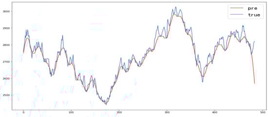
Figure 8.
ARIMA model prediction results.
Table 4.
ARIMA model predicted results index value.
It can be concluded that the results of the evaluation metrics RMSE, MAPE, and for the corn settlement price are acceptable. Combined with the charts, it can be inferred that the predictive performance achieved by using the ARIMA model for corn price forecasting is moderately satisfactory. Compared to the results of the LSTM model, the ARIMA model performs better, but it is not as suitable as the LSTM model based on Bézier fitting. Further optimization of this model is needed to improve its predictive accuracy and precision.
3.5. SVR Model Construction and Predictive Analysis
Prediction steps: ① Divide the corn futures price data into training and testing sets in an 8:2 ratio. ② Choose a kernel function to establish the Support Vector Machine (SVM) model. Select the Gaussian kernel function (rbf). ③ Input the training data and initialize the penalty factor parameter C and the parameter gamma. ④ Based on the initialized parameters, determine the approximate range of parameters and finalize the model parameters. ⑤ Input the testing set data and compare the predicted results with the actual corn futures prices for analysis.
Therefore, through calculation and parameter optimization, it is found that setting the prediction step length to 1 and using the first 50 data points to predict the next data point results in a small error. Initially, the penalty factor parameter is set to 1, 3, 5, 10, 30, and 100, and the parameter gamma is set to 0.001, 0.005, 0.05, 0.1, 0.15, 0.5, and 0.8. The rbf kernel function is selected, and the final parameters are determined to be and gamma = 0.15. Using these parameters, the testing set data are predicted, and the prediction results are shown in Figure 9, and the index results are shown in Table 5.
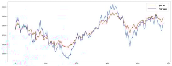
Figure 9.
SVR model prediction results.
Table 5.
Index value of prediction result based on SVR model.
Based on the prediction results, it can be concluded that the SVR model based on corn settlement price performs well in predicting the overall price trend and features. However, it may not accurately predict some abrupt price trends, resulting in relatively smoother prediction results. Considering the evaluation metrics RMSE, MAPE, and Dstat, it can be observed that the results of all three metrics are acceptable. The predictive performance is moderate, with the MAPE and RMSE metrics lacking high precision. However, the metric performs better compared to LSTM and ARIMA models but inferior to the predictive results of the LSTM model based on Bézier fitting. Further optimization of this model is required to enhance its predictive accuracy and precision.
3.6. VMD-LSTM Model Construction and Predictive Analysis
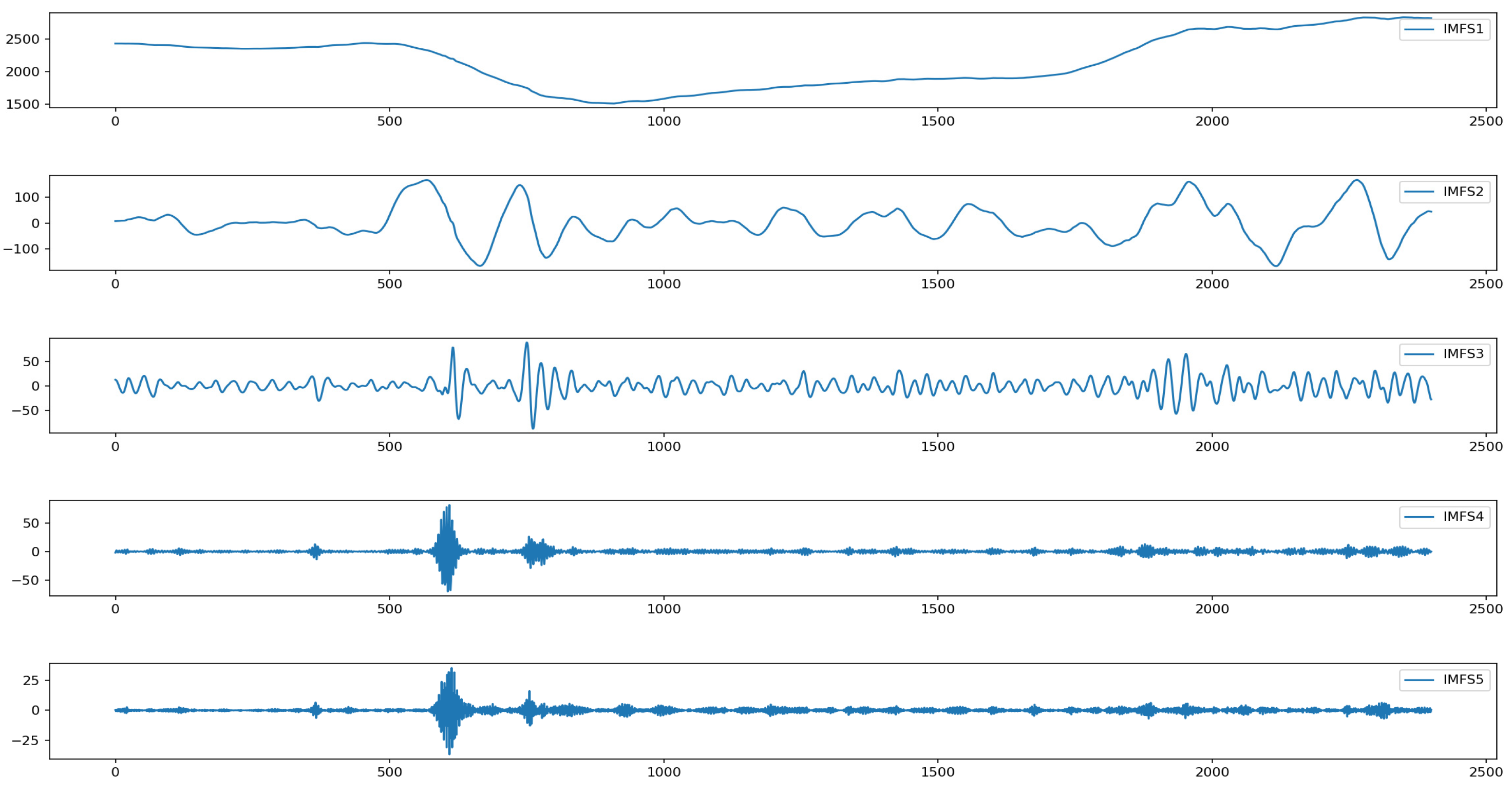
The original time series data are decomposed using VMD, and then the decomposed data are used for prediction. Finally, the prediction results are added together to reconstruct the prediction results of the original data and are compared with the original data. Prediction steps: (1). The daily futures price data of corn were divided into a training set and a test set according to the ratio of 8:2. (2). After several parameter adjustments, VMD parameters are determined: alpha = 2400, tau = 0, K = 5, DC = 0, init = 1, tol = 1 × 10⁻⁷. The breakdown results are shown in Figure 10.
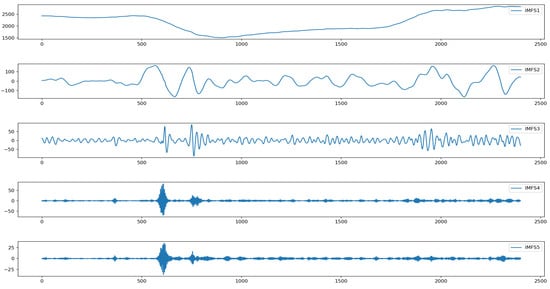
Figure 10.
VMD decomposition result diagram.
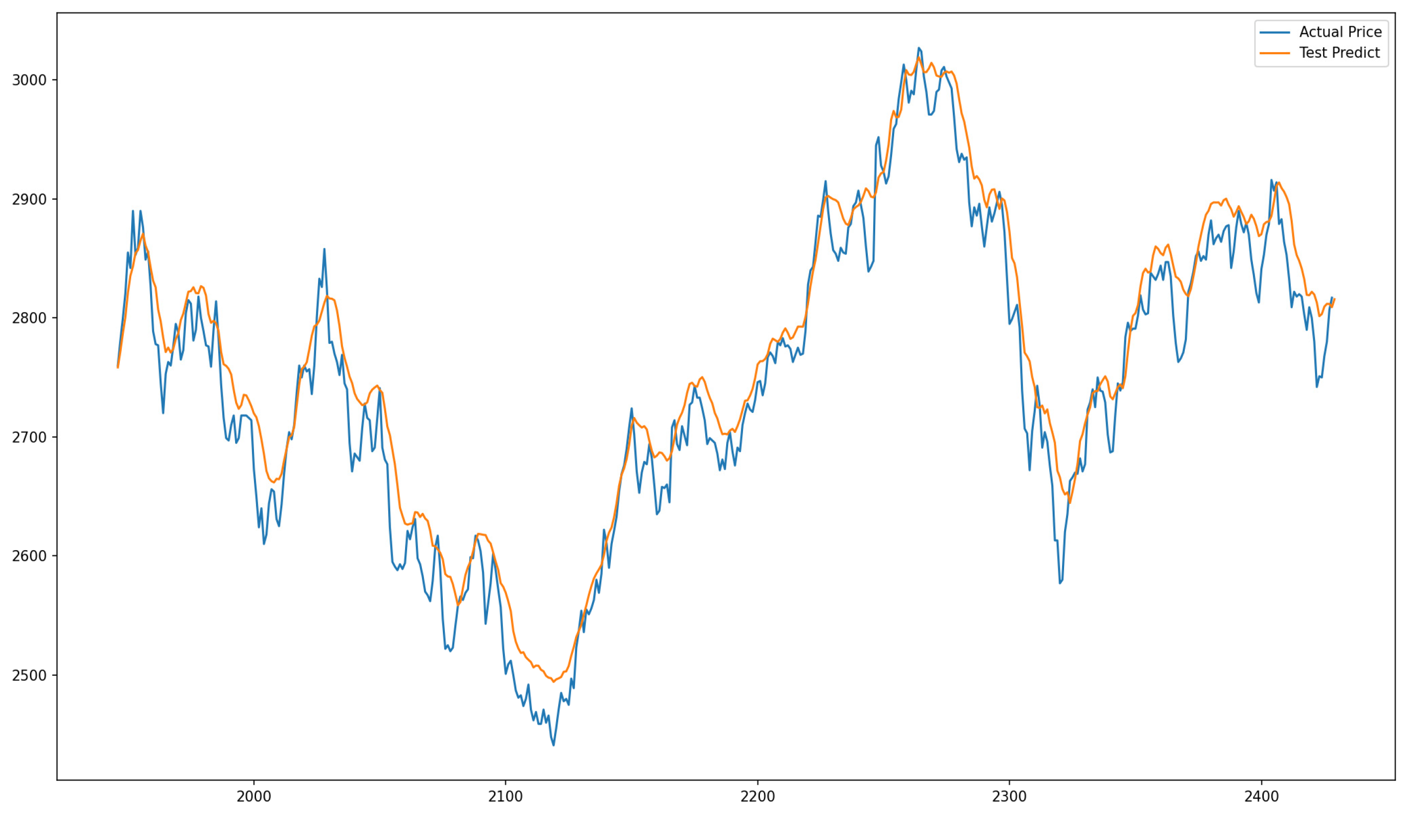
(3): Input the decomposed VMD data into the LSTM network as training data, set the output layer dimension to 1, and use RMSE as an evaluation index to continuously evaluate and optimize the parameters by cross-validation. The hidden layer is set to 3, the number of iterations is 2000, and the historical time step is 2. (4): Bring in the test set data and compare and analyze the forecast results with the actual price data of corn futures. Forecast results and indicator results are shown in Figure 11 and Table 6.
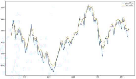
Figure 11.
VMD + LSTM prediction graph.
Table 6.
Index value of prediction result based on VMD + LSTM model.
According to the forecast result chart, it can be concluded that the settlement price of corn based on the VMD + LSTM model has a suitable prediction effect on the overall price trend and characteristics. Combined with the evaluation indexes RMSE, MAPE, and , it can be seen that the results of the three indexes are all OK, and the prediction effect is better, but the index is only better than LSTM. It shows that VMD can predict the price of corn price well after time series decomposition but cannot learn the trend of rising and falling. Further optimization of this model is needed to improve the prediction accuracy and accuracy of the model.
3.7. Comparison of Results
Based on the displayed prediction results of corn futures prices, it is observed that the predicted values from various methods are generally close to the actual values. This indicates that the selected prediction methods for corn price forecasting are relatively reasonable. However, compared to other methods, the predictive performance of the LSTM model based on Bézier curves demonstrates better accuracy and precision in predicting corn prices. The comparison results of the above five models are shown in Table 7.
Table 7.
The index value of different model prediction results.
According to the calculation results in the above table, it is observed that compared with LSTM, ARIMA, and SVR models, the RMSE index of the Bezier curve-based LSTM method and VMD decomposition-based LSTM method is much lower, the MAPE index is also significantly reduced, and the prediction of price trend is more accurate. It can be judged that there are certain advantages in the prediction after noise elimination of the original data, and the prediction accuracy is also significantly improved. Through the analysis of the daily price characteristics of corn and the comprehensive consideration of the forecast results, combined with the characteristics of the prediction accuracy and the practicability of the method, it can be concluded that the combination of Bezier curve fitting and LSTM model is a better choice to forecast the price, which has certain practicability and feasibility.
It is concluded that the possible reason for the best performance of ARIMA among the three original models is that ARIMA itself has undergone white noise detection and stationarity tests. Compared with the other two basic models, ARIMA has carried out data preprocessing so that the subsequent models can better fit the data. It has been proved that prediction after noise treatment can improve the accuracy of prediction, which is demonstrated by Bezier + LSTM and VMD + LSTM. The problem that the direction index value of VMD + LSTM is low and fails to meet the expectations may be caused by the error of the forecast result after decomposition. The forecast result of VMD + LSTM is reconstructed by adding the forecast results of each decomposed curve, and there are errors in each prediction, which may be that although MAPE is relatively ideal, the reason why the value is not ideal.
4. Conclusions
This paper focuses on using different predictive modeling methods to forecast corn futures daily price data and analyzes whether the proposed forecasting methods have higher accuracy, better predictive performance, and practical application significance.
In the study of corn daily price prediction, we use the Bezier curve fitting method to process the data set by constantly adjusting the control vertex to change the curve shape and combine the method of long-term memory network (LSTM) to forecast and analyze the corn daily price data. According to the calculated signal-to-noise ratio and the characteristics of corn daily price data, the B-spline multi-layer vertex fitting method is selected for de-noising processing, and the de-noised data are combined with the LSTM model for prediction analysis. The results of LSTM, ARIMA, and SVR model prediction are compared with the original data as input values, and the results of combined prediction with the LSTM model after VMD decomposition and denoising are also compared. It is concluded that the prediction effect of the LSTM model based on Bezier is obviously better and has greater practical significance.
This study provides new ideas and methods for price prediction of corn and other related agricultural products. Through big data technology, price prediction can be conducted more effectively and scientifically, which has practical significance. This modeling approach can be extended to the prediction of prices of more agricultural products, thereby better analyzing the price trends of agricultural products and providing reasonable and effective suggestions for government decision-making and the determination of target prices for agricultural products, thus better safeguarding the interests of farmers regarding the sale of agricultural products.
Author Contributions
Conceptualization, Q.Z., J.C., X.F. and Y.W.; Methodology, Q.Z., J.C., X.F. and Y.W.; Investigation, Q.Z., J.C., X.F. and Y.W.; Data curation, Q.Z., J.C. and X.F.; Writing—original draft, J.C. and X.F.; Writing—review and editing, Q.Z., J.C., X.F. and Y.W.; Supervision, Q.Z. and Y.W. All authors have read and agreed to the published version of the manuscript.
Funding
This research is supported by the Funds for First-class Discipline Construction (XK1802-5).
Data Availability Statement
The original contributions presented in the study are included in the article, further inquiries can be directed to the corresponding author.
Conflicts of Interest
The authors declare no conflicts of interest.
References
- Akkem, Y.; Biswas, S.K.; Varanasi, A. Smart farming using artificial intelligence: A review. Eng. Appl. Artif. Intell. 2023, 120, 105899. [Google Scholar] [CrossRef]
- Feng, Y.; Mei, D.; Zhao, H. Auction-based deep learning-driven smart agricultural supply chain mechanism. Appl. Soft Comput. 2023, 149, 111009. [Google Scholar] [CrossRef]
- Deléglise, H.; Interdonato, R.; Bégué, A.; D’hôtel, E.M.; Teisseire, M.; Roche, M. Food security prediction from heterogeneous data combining machine and deep learning mSethods. Expert Syst. Appl. 2022, 190, 116189. [Google Scholar] [CrossRef]
- Kumar, P.; Sandip, G. Wavelets based artificial neural network technique for forecasting agricultural prices. J. Indian Soc. Probab. Stat. 2022, 23, 47–61. [Google Scholar]
- Atalan, A. Forecasting drinking milk price based on economic, social, and environmental factors using machine learning algorithms. Agribusines 2023, 39, 214–241. [Google Scholar] [CrossRef]
- Ren, W.; Li, B.; Han, M. A novel granger causality method based on HSIC-Lasso for revealing nonlinear relationship between multivariate time series. Phys. A Stat. Mech. Its Appl. 2020, 541, 123245. [Google Scholar] [CrossRef]
- Weng, Y.; Wang, X.; Hua, J.; Wang, H.; Kang, M.; Wang, F. Forecasting horticultural products price using ARIMA model and neural network based on a large-Scale data set collected by web crawler. IEEE Trans. Comput. Soc. Syst. 2019, 6, 547. [Google Scholar] [CrossRef]
- Varun, R.; Neema, N.; Sahana, H. Agriculture commodity price forecasting using Ml techniques. Int. J. Innov. Technol. Explor. Eng. 2019, 9, 729–732. [Google Scholar]
- Brandt, A.; Bessler, D. Price forecasting and evaluation: An application in agriculture. J. Forecast. 1983, 2, 237–248. [Google Scholar] [CrossRef]
- Purohit, S.; Panigrahi, S.; Sethy, P.; Behera, S. Time series forecasting of price of agricultural products using hybrid methods. Appl. Artif. Intell. 2021, 35, 1388–1406. [Google Scholar] [CrossRef]
- Raflesia, S.; Taufiqurrahman, T.; Iriyani, S.; Lestarini, D. Agricultural commodity price forecasting using pso-rbf neural network for farmers exchange rate improvement in Indonesia. Indones. J. Electr. Eng. Inform. 2021, 9, 784–792. [Google Scholar] [CrossRef]
- Zhao, H. Futures price prediction of agricultural products based on machine learning. Neural Comput. Appl. 2021, 33, 837–850. [Google Scholar] [CrossRef]
- Liu, J.; Zhang, B.; Zhang, T.; Wang, J. Soybean futures price prediction model based on EEMD-NAGU. IEEE Access 2023, 11, 99328. [Google Scholar] [CrossRef]
- Sarpong-Streetor, R.M.N.Y.; Sokkalingam, R.; Othman, M.; Azad, A.S.; Syahrantau, G.; Arifin, Z. Intelligent hybrid ARIMA-NARNET time series model to forecast coconut price. IEEE Access 2023, 11, 48568–48577. [Google Scholar] [CrossRef]
- Weiping, L.; Chengzhu, W.; Yonggang, L.; Yishun, L.; Keke, H. Ensemble forecasting for product futures prices using variational mode decomposition and artificial neural networks. Chaos Solitons Fractals 2021, 146, 110822. [Google Scholar]
- Zhang, G. Time series forecasting using a hybrid ARIMA and neural network model. Neurocomputing 2003, 50, 159. [Google Scholar] [CrossRef]
- Gu, Y.; Jin, D.; Yin, H.; Zheng, R.; Piao, X.; Yoo, S. Forecasting agricultural commodity prices using dual input attention LSTM. Agriculture 2022, 12, 256. [Google Scholar] [CrossRef]
- Ray, S.; Lama, A.; Mishra, P.; Biswas, T.; Sankar Das, S.; Gurung, B. An ARIMA-LSTM model for predicting volatile agricultural price series with random forest technique. Appl. Soft Comput. 2023, 149, 110939. [Google Scholar] [CrossRef]
- Simões, N.; Wang, L.; Ochoa-Rodriguez, S.; Leitão, J.P.; Pina, R.; Onof, C.; David, L.M. A coupled SSA-SVM technique for stochastic short-term rainfall forecasting. J. Environ. Sci. Eng. Comput. Sci. (JECET) 2011. Available online: https://api.semanticscholar.org/CorpusID:106504054 (accessed on 1 June 2024).
- Sivapragasam, C.; Liong, S.; Pasha, M. Rainfall and runoff forecasting with SSA–SVM approach. J. Hydroinform. 2001, 3, 141–152. [Google Scholar] [CrossRef]
- Paul, R.K.; Yeasin, M.; Kumar, P.; Kumar, P.; Balasubramanian, M.; Roy, H.S.; Gupta, A. Machine learning techniques for forecasting agricultural prices: A case of brinjal in Odisha, India. PLoS ONE 2022, 17, e0270553. [Google Scholar] [CrossRef]
- Krishna, B.M.; Satyanarayana, S.V.V.; Satyanarayana, P.V.V.; Suman, M.V. Improving time–frequency resolution in non-stationary signal analysis using a convolutional recurrent neural network. Signal Image Video Process. 2023, 18, 4797–4810. [Google Scholar] [CrossRef]
- Bai, Z.; Pang, H.; He, Z.; Zhao, B.; Wang, T. Path Planning of Autonomous Mobile Robot in Comprehensive Unknown Environment Using Deep Reinforcement Learning. IEEE Internet Things J. 2024, 11, 22153–22166. [Google Scholar] [CrossRef]
- Huang, Y.; Yan, L.; Cheng, Y.; Qi, X.; Li, Z. Coal Thickness Prediction Method Based on VMD and LSTM. Electronics 2022, 11, 232. [Google Scholar] [CrossRef]
- Otero, J.F.A.; López-De-Ipina, K.; Caballer, O.S.; Marti-Puig, P.; Sánchez-Méndez, J.I.; Iradi, J.; Bergareche, A.; Solé-Casals, J. EMD-based data augmentation method applied to handwriting data for the diagnosis of Essential Tremor using LSTM networks. Sci. Rep. 2022, 12, 12819. [Google Scholar] [CrossRef]
- Lagi, M.; Bertrand, K.Z.; Bar-Yam, Y. Accurate market price formation model with both supply-demand and trend-following for global food prices providing policy recommendations. Proc. Natl. Acad. Sci. USA 2015, 112, 6119–6128. [Google Scholar] [CrossRef]
- Xu, X.; Zhang, Y. Corn cash price forecasting with neural networks. Comput. Electron. Agric. 2021, 184, 106120. [Google Scholar] [CrossRef]
- Kantanantha, N.; Serban, N.; Griffin, P. Yield and price forecasting for stochastic crop decision planning. J. Agric. Biol. Environ. Stat. 2010, 15, 362–380. [Google Scholar] [CrossRef]
- Farin, G. Algorithms for rational Bézier curves. Comput. Aided Des. 1983, 15, 73–77. [Google Scholar] [CrossRef]
- Wang, Y.; Shi, X.; Xi, P.; Lang, H. Quasi-distribution appraisal about finite element analysis of multi-functional structure made of honeycomb sandwich materials. J. Wuhan Univ. Technol. Mater. Sci. Ed. 2018, 33, 30–34. [Google Scholar] [CrossRef]
- Delgado, J.; Peña, J. Geometric properties and algorithms for rational q-Bézier curves and surfaces. Mathematics 2020, 8, 541. [Google Scholar] [CrossRef]
- Wang, Y.; Hu, B.; Xi, P.; Xue, W. A note on variable upper limit integral of Bézier curve. Adv. Sci. Lett. 2011, 4, 1815–1819. [Google Scholar] [CrossRef]
- Li, Y.; Fang, L.; Zheng, Z.; Cao, J. On control polygons of planar sextic pythagorean hodograph curves. Mathematics 2023, 11, 383. [Google Scholar] [CrossRef]
- Jaiswal, R.; Girish, K.; Kumar, R.; Choudhary, K. Deep long short-term memory based model for agricultural price forecasting. Neural Comput. Appl. 2021, 34, 4661. [Google Scholar] [CrossRef]
- Gers, F.; Schraudolph, N.; Schmidhuber, J. Learning precise timing with LSTM recurrent networks. J. Mach. Learn. Res. 2002, 3, 115–143. [Google Scholar]
- Shu, X.; Zhang, L.; Sun, Y.; Tang, J. Host-parasite: Graph LSTM-in-LSTM for group activity recognition. IEEE Trans. Neural Netw. Learn. Syst. 2021, 32, 663. [Google Scholar] [CrossRef] [PubMed]
- Yang, Y.; Zhou, J.; Ai, J.; Bin, Y.; Hanjalic, A.; Shen, H.T.; Ji, Y. Video captioning by adversarial LSTM. IEEE Trans. Image Process. 2018, 27, 5600. [Google Scholar] [CrossRef]
- Houdt, G.; Mosquera, C.; Gonzalo, N. A review on the long short-term memory model. Artif. Intell. Rev. 2020, 53, 5929–5955. [Google Scholar] [CrossRef]
- Al-Musaylh, M.; Deo, R.; Adamowski, J.; Li, Y. Short-term electricity demand forecasting with MARS, SVR and ARIMA models using aggregated demand data in Queensland, Australia. Adv. Eng. Inform. 2018, 35, 1–16. [Google Scholar] [CrossRef]
- Gilbert, K. An ARIMA supply chain model. Manag. Sci. 2005, 51, 305–310. [Google Scholar] [CrossRef]
- Piccolo, D. A distance measure for classifying ARIMA models. J. Time Ser. Anal. 1990, 11, 153–164. [Google Scholar] [CrossRef]
- Mengjiao, Q.; Zhihang, L.; Zhenhong, D. Red tide time series forecasting by combining ARIMA and deep belief network. Knowl. Based Syst. 2017, 125, 39–52. [Google Scholar]
- Ho, S.; Xie, M. The use of ARIMA models for reliability forecasting and analysis. Comput. Ind. Eng. 1998, 35, 213–216. [Google Scholar] [CrossRef]
- Wu, X.; Zuo, W.; Lin, L.; Jia, W.; Zhang, D. F-SVM: Combination of feature transformation and SVM learning via convex relaxation. IEEE Trans. Neural Netw. Learn. Syst. 2018, 29, 5185. [Google Scholar] [CrossRef] [PubMed]
- Barbu, T. CNN-based temporal video segmentation using a nonlinear hyperbolic PDE-based multi-scale analysis. Mathematics 2023, 11, 245. [Google Scholar] [CrossRef]
- Jingxue, B.; Meiqi, Z.; Guobiao, Y.; Hongji, C.; Yougui, F.; Hu, J.; Dashuai, C. PSOSVRPos: WiFi indoor positioning using SVR optimized by PSO. Expert Syst. Appl. 2023, 222, 119778. [Google Scholar]
- Brereton, G.; Lloyd, R. Support vector machines for classification and regression. Analyst 2010, 135, 230–267. [Google Scholar] [CrossRef] [PubMed]
- Zhao, Q.; Feng, X.; Zhang, L.; Wang, Y. Research on short-term passenger flow prediction of LSTM rail transit based on wavelet denoising. Mathematics 2023, 11, 4204. [Google Scholar] [CrossRef]
- Yanxue, W.; Richard, M.; Jiawei, X.; Weiguang, Z. Research on variational mode decomposition and its application in detecting rub-impact fault of the rotor system. Mech. Syst. Signal Process. 2015, 243, 60–61. [Google Scholar]
- Xiong, T.; Li, M.; Cao, J. Do futures prices help forecast spot prices? evidence from China’s new live hog futures. Agriculture 2023, 13, 1663. [Google Scholar] [CrossRef]
- Qinghua, G.; Yinxin, C.; Naixue, X.; Lu, C. Forecasting Nickel futures price based on the empirical wavelet transform and gradient boosting decision trees. Appl. Soft Comput. 2021, 109, 107472. [Google Scholar]
- Sarbajit, P.; Pankaj, G.; Biswas, P. Cubic Bézier approximation of a digitized curve. Pattern Recognit. 2007, 40, 2730–2741. [Google Scholar]


Disclaimer/Publisher’s Note: The statements, opinions and data contained in all publications are solely those of the individual author(s) and contributor(s) and not of MDPI and/or the editor(s). MDPI and/or the editor(s) disclaim responsibility for any injury to people or property resulting from any ideas, methods, instructions or products referred to in the content. |
© 2024 by the authors. Licensee MDPI, Basel, Switzerland. This article is an open access article distributed under the terms and conditions of the Creative Commons Attribution (CC BY) license (https://creativecommons.org/licenses/by/4.0/).