Linearly Implicit Conservative Schemes with a High Order for Solving a Class of Nonlocal Wave Equations

Abstract

This paper introduces a class of novel high-accuracy energy-preserving numerical schemes tailored specifically for solving the nonlocal wave equation with Gaussian kernel, which plays a fundamental role in various scientific and engineering applications where traditional local wave equations are inadequate. Comprehensive numerical experiments, including comparisons with analytical solutions and benchmark tests, demonstrate the superior accuracy and energy-preserving capabilities of the proposed schemes. These high-accuracy energy-preserving schemes represent a valuable tool for researchers and practitioners in fields reliant on nonlocal wave equation modeling, offering enhanced predictive capabilities and robustness in capturing complex wave dynamics while ensuring long-term numerical stability.

1. Introduction

The nonlocal wave equation is a mathematical model used to describe wave propagation phenomena that exhibit nonlocal behavior [1]. The equations are often preferred over traditional local wave equations for certain problems because they can capture interactions over a distance, which local equations cannot. This nonlocality can model more complex behaviors and phenomena more accurately [2,3]. For example, nonlocal wave equations are better at modeling material properties where interactions are not limited to adjacent particles but can span over a range of distances [4]. In the current paper, we mainly consider the computation of the d-dimensional ($d=1,2$) nonlocal wave equation with the following form

$$\left\{\begin{array}{cc}{\partial }_t^{2}u(\mathit{x},t)=-{\mathcal{L}}_{\delta }u(\mathit{x},t)-f\left(u\right),\hfill & \hspace{1em}\hspace{1em}\hspace{1em}\mathit{x}\in \mathsf{\Omega },t>0,\\ u(\mathit{x},0)=u_0\left(\mathit{x}\right),{\partial }_{t}u(\mathit{x},0)={\tilde{u}}_0\left(\mathit{x}\right),\hfill & \mathit{x}\in \overline{\mathsf{\Omega }},\end{array}\right.$$

(1)

where $\mathsf{\Omega }={\displaystyle \prod _{i=1}^d}(-L_i,L_i)$ in ${\mathbb{R}}^d$$(d=1,2)$, $u(\mathit{x},t)$ is the wave field, representing displacement or some other quantity, as a function of position $\mathit{x}$ and time t. The nonlinear term $f\left(u\right)=F^{\prime }\left(u\right)$ satisfies the Lipschitz condition, the given functions $u_0,{\tilde{u}}_0$ are smooth and compactly supported on $\mathsf{\Omega }$, and ${\mathcal{L}}_{\delta }$ is the nonlocal operator and has the form [2]

$$\begin{array}{c}\hfill {\mathcal{L}}_{\delta }u\left(\mathit{x}\right):={\int }_{\mathsf{\Omega }}{J}_{\delta }(\mathit{x}-\mathit{y})\left(u\left(\mathit{x}\right)-u\left(\mathit{y}\right)\right)\mathrm{d}\mathit{y}=(J_{\delta }\ast 1)u-J_{\delta }\ast u,u\in L^2\left(\mathsf{\Omega }\right),\end{array}$$

(2)

where $J_{\delta }(\mathit{x}-\mathit{y})$ is kernel function that represents the nonlocalis kernel function that represents the nonlocal interaction between points $\mathit{x}$ and $\mathit{y}$, “∗” stands for the periodic convolution, and

$$\begin{array}{c}\hfill (J_{\delta }\ast u)\left(\mathit{x}\right)={\int }_{\mathsf{\Omega }}{J}_{\delta }(\mathit{x}-\mathit{y})u\left(\mathit{y}\right)d\mathit{y}={\int }_{\mathsf{\Omega }}{J}_{\delta }\left(\mathit{y}\right)u(\mathit{x}-\mathit{y})d\mathit{y},\end{array}$$

(3)

the integral term on the right-hand side accounts for the nonlocal effects, representing the influence of the field at nearby points on the behavior of the wave at a given point. The choice of the kernel function J determines the specific nonlocal behavior of the system. Nonlocal wave equations arise in various fields of physics and engineering, including solid mechanics, fluid dynamics, and electromagnetics, where phenomena such as wave dispersion, long-range interactions, and memory effects need to be considered. They are also of interest in mathematical analysis due to their rich mathematical structure and challenging properties. The paper considers the Gaussian kernel $J_{\delta }$ with the form [3]

$$\begin{array}{c}\hfill J_{\delta }\left(\mathit{x}\right)={\displaystyle \frac{4}{{\pi }^{d/2}{\delta }^{d+2}}}{\mathrm{e}}^{-{\displaystyle \frac{{\left|\mathit{x}\right|}^2}{{\delta }^2}}},\mathit{x}\in {\mathbb{R}}^d,\delta >0,\end{array}$$

(4)

and satisfies

$$\begin{array}{c}\hfill C_{\delta }:={\int }_{{\mathbb{R}}^d}{J}_{\delta }\left(\mathit{x}\right)\mathrm{d}\mathit{x}={\displaystyle \frac{4}{{\delta }^2}},{\int }_{{\mathbb{R}}^d}{J}_{\delta }\left(\mathit{x}\right){\left|\mathit{x}\right|}^2\mathrm{d}\mathit{x}=2d,\end{array}$$

(5)

the system (1) can conserve the following energy conservation law based on the positive definiteness of the operator ${\mathcal{L}}_{\delta }$, namely

$$\begin{array}{cc}\hfill & \mathcal{H}\left(t\right):={\int }_{\mathsf{\Omega }}\left({\displaystyle \frac{1}{2}}{\left|{\partial }_{t}u\right|}^2+{\displaystyle \frac{1}{2}}{\int }_{\mathsf{\Omega }}{J}_{\delta }(\mathit{x}-\mathit{y}){\left(u(\mathit{x},t)-u(\mathit{y},t)\right)}^2\mathrm{d}\mathit{y}+F\left(u\right)\right)d\mathit{x}\equiv \mathcal{H}\left(0\right),\hfill \end{array}$$

(6)

which can be rewritten as a simple form and is usually called Hamiltonian energy

$$\begin{array}{cc}\hfill & \mathcal{H}\left(t\right)={\int }_{\mathsf{\Omega }}\left({\displaystyle \frac{1}{2}}{\left|{\partial }_{t}u\right|}^2+{\displaystyle \frac{1}{2}}|{\mathcal{L}}_{\delta }^{{\displaystyle \frac{1}{2}}}u{|}^2+F\left(u\right)\right)d\mathit{x},\mathrm{with}({\mathcal{L}}_{\delta }^{{\displaystyle \frac{1}{2}}}u,{\mathcal{L}}_{\delta }^{{\displaystyle \frac{1}{2}}}u)=({\mathcal{L}}_{\delta }u,u),\hfill \end{array}$$

(7)

where $\left(•,★\right):={\int }_{\mathsf{\Omega }}•★d\mathit{x}$.

In recent years, several numerical algorithms have been proposed to address the challenge of obtaining analytical solutions for various nonlocal equations [5,6,7]. However, these algorithms fail to uphold the conservative laws of the equation and are unsuitable for long-term numerical computations. Drawing inspiration from the concept of structure-preserving algorithms for classical Hamiltonian systems, researchers have developed numerous conservative schemes for nonlocal systems. For instance, Wang and Xiao [8,9,10] derived invariants of the nonlocal Schrödinger and devised finite difference schemes to conserve these invariants, with discussions on the existence and uniqueness of solutions, and the convergence of schemes in their works. Ref. [4] presented the energy conservation law for the nonlocal wave equation with Riesz fractional derivatives, and scholars developed corresponding structure-preserving schemes for the equation [11,12]. Wang and Li developed a dissipation-preserving finite difference scheme for the wave equation with integral fractional Laplacian [13,14]. Other structure-preserving schemes can also be applied to nonlocal wave equations, such as the averaged vector field method [15] and implicit–explicit relaxation Runge–Kutta methods (readers can refer to references [16,17]).

Unfortunately, these numerical schemes mentioned above only have second-order accuracy in temporal. Due to the low-order nature of these methods, they may exhibit poor accuracy, particularly when modeling complex physical phenomena or capturing fine details in the solution. Over the past decade, some numerical methods have been proposed to construct high-accuracy conservative methods for conservative systems [18,19]. But, these schemes are fully implicit, which often require solving nonlinear systems of equations at each time step, which can significantly increase the computational cost, making them computationally expensive for large-scale simulations. Linearly implicit schemes offer computational advantages over fully implicit schemes. They strike a balance between computational efficiency and accuracy, making them suitable for large-scale simulations on modern computing architectures. Therefore, it is expected to construct and analyze high-accuracy linearly implicit conservative numerical schemes for the nonlocal wave equation. Recently, Li developed a novel auxiliary variable method based on the ideas of the scalar auxiliary variable (SAV) method [20,21], namely the exponential scalar auxiliary variable (ESAV) approach, which removes the definition restriction that auxiliary variables can only be square root functions. The definition form of the auxiliary variable is applicable to any reversible function for the ESAV approach [22], as treating the new auxiliary variable explicitly can derive a class of linear, no-iterative, energy-stable schemes for dissipative systems.

The symplectic Runge–Kutta method excels in preserving the energy and geometric properties of Hamiltonian systems, ensuring long-term stability and accuracy in numerical simulations [23]. These advantages provide us with a framework for constructing high-accuracy conservation schemes. The motivation behind the paper is to leverage the ESAV method in combination with the Runge–Kutta method to construct high-accuracy, linearly implicit conservative numerical schemes for the nonlocal wave equation. This approach aims to do the following: (I) Develop linearly implicit high-order schemes that can efficiently obtain numerical solutions. (II) Ensure the schemes preserve the system’s energy, providing high stability in numerical simulations. In summary, the work seeks to create an effective numerical method that balances accuracy and computational efficiency, suitable for large-scale simulations while preserving the intrinsic energy properties of the modeled systems. Unfortunately, the convergence analysis of the proposed schemes has not been discussed, which is the focus of our future work.

The paper is structured as follows: In Section 2, an equivalent system for the nonlocal wave equation is presented through the introduction of auxiliary variables. Section 3 utilizes the symplectic Runge–Kutta method to derive a high-accuracy linearly implicit scheme for the equivalent system in the time direction, based on extrapolation technology, and examines its conservation properties. Section 4 showcases numerical results to illustrate the theoretical findings. Finally, conclusions are drawn in the last section.

2. Equivalent System with ESAV Approach

We introduce an auxiliary variable:

$$q(u,t)=exp\left({\displaystyle \frac{{\int }_{\mathsf{\Omega }}F\left(u\right)d\mathit{x}}{\mathcal{C}}}\right),$$

(8)

where $\mathcal{C}$ is a normal number; for simplicity, we take $\mathcal{C}=1$, and the original Hamilton energy can be transformed into the following form

$$\mathcal{E}[u,v,q]={\int }_{\mathsf{\Omega }}\left({\displaystyle \frac{1}{2}}{v}^2+{\displaystyle \frac{1}{2}}|{\mathcal{L}}_{\delta }^{{\displaystyle \frac{1}{2}}}u{|}^2\right)d\mathit{x}+ln\left(q\right).$$

(9)

and obtain

$$\begin{array}{c}\hfill {\displaystyle \frac{dq}{dt}}={\displaystyle \frac{dexp\left({\int }_{\mathsf{\Omega }}F\left(u\right)d\mathit{x}\right)}{dt}}=exp\left({\int }_{\mathsf{\Omega }}F\left(u\right)d\mathit{x}\right){\int }_{\mathsf{\Omega }}f\left(u\right)u_{t}d\mathit{x},\end{array}$$

(10)

according to the energy variational principle, we have rewritten the nonlocal wave Equation (1) into a new equivalent system, namely

$$\begin{array}{cc}\hfill & u_t=v,\hfill \end{array}$$

(11)

$$\begin{array}{cc}\hfill & v_t=-{\mathcal{L}}_{\delta }u(\mathit{x},t)-{\displaystyle \frac{f\left(u\right)}{exp\left({\int }_{\mathsf{\Omega }}F\left(u\right)d\mathit{x}\right)}}q,\hfill \end{array}$$

(12)

$$\begin{array}{cc}\hfill & q_t=exp\left({\int }_{\mathsf{\Omega }}F\left(u\right)d\mathit{x}\right){\int }_{\mathsf{\Omega }}f\left(u\right)u_{t}d\mathit{x},\hfill \end{array}$$

(13)

with the consistent initial condition

$$\begin{array}{c}\hfill u(\mathit{x},0)=u_0\left(\mathit{x}\right),v(\mathit{x},0)=v_0\left(\mathit{x}\right),q_0:=exp\left({\int }_{\mathsf{\Omega }}F\left(u_0\right)d\mathit{x}\right),\end{array}$$

(14)

to simplify the notation, we define

$$\begin{array}{c}\hfill {\mathcal{A}}^{q,u}:={\displaystyle \frac{f\left(u\right)}{exp\left({\int }_{\mathsf{\Omega }}F\left(u\right)d\mathit{x}\right)}}q,\end{array}$$

(15)

then, system (11)–(13) can be rewritten as the following simple form

$$\begin{array}{cc}\hfill & u_t=v,\hfill \end{array}$$

(16)

$$\begin{array}{cc}\hfill & v_t=-{\mathcal{L}}_{\delta }u-{\mathcal{A}}^{q,u},\hfill \end{array}$$

(17)

$$\begin{array}{cc}\hfill & {\displaystyle \frac{d}{dt}}ln\left(q\right)=\left({\mathcal{A}}^{q,u},u_t\right).\hfill \end{array}$$

(18)

Next, we focus on studying the conservation properties of the reformulated system (16)–(18).

Theorem 1. 

Under the periodic boundary condition, systems (16)–(18) possess the following modified energy conservation law

$$\begin{array}{c}\hfill {\displaystyle \frac{d}{dt}}\mathcal{E}[u,v,q]=0,\end{array}$$

(19)

here $\mathcal{E}[u,v,q]$ is given by (9).

Proof. 

Taking the inner products of system (16) and (17) with $v_t$ and v, respectively, we obtain that

$$\begin{array}{c}\hfill \left(u_t,v_t\right)=\left(v,v_t\right),\end{array}$$

(20)

and

$$\begin{array}{c}\hfill \left(v_t,v\right)=\left(-{\mathcal{L}}_{\delta }u,v\right)-\left({\mathcal{A}}^{q,u},v\right).\end{array}$$

(21)

Combining (20) and (21), we obtain the following energy conservation law

$$\begin{array}{c}\hfill {\displaystyle \frac{d}{dt}}\left[{\int }_{\mathsf{\Omega }}\left({\displaystyle \frac{1}{2}}{v}^2+{\displaystyle \frac{1}{2}}|{\mathcal{L}}_{\delta }^{{\displaystyle \frac{1}{2}}}u{|}^2\right)d\mathit{x}+ln\left(q\right)\right]=0.\end{array}$$

(22)

The proof is completed. □

3. Semi-Discrete Fourier Pseudo-Spectral Conservative System

3.1. Fourier Pseudo-Spectral Method for the Nonlocal Operator

Space discretization, illustrated here with a one-dimensional example, can be extended to high-dimensional cases [2]. For positive even integers $\mathcal{N}$ and N, the step sizes in space are defined by $h={\displaystyle \frac{2L}{\mathcal{N}}}$, and the time step $\tau :={\displaystyle \frac{T}{N}}$. Then, we set ${\mathsf{\Omega }}_h=\left\{x_i\right|x_i=-L+ih,$ $0\le i\le \mathcal{N}-1\}$ and define

$$\begin{array}{cc}\hfill & \mathit{u}={(u_0,u_1,\cdots ,u_{\mathcal{N}-1})}^T.\hfill \end{array}$$

The discrete inner product and $L^{\infty }$-norm are given as

$$\begin{array}{c}\hfill {\langle \mathit{u},\mathit{\psi }\rangle }_h=h\sum _{i=0}^{\mathcal{N}-1}{u}_i{\overline{\psi }}_i,\parallel \mathit{u}\parallel ={\langle \mathit{u},\mathit{u}\rangle }_h^{{\displaystyle \frac{1}{2}}}{,\parallel \mathit{u}\parallel }_{\infty }=\underset{x_i\in {\mathsf{\Omega }}_h}{sup}\left|u_i\right|.\end{array}$$

In practical computation, the nonlocal operator $\mathcal{L}$ can be approximated by the Fourier-pseudo spectral method, namely [24]

$$\begin{array}{cc}\hfill \left(-{\mathcal{L}}_{\delta }{u}_{\mathcal{N}}\right)\left(x_j\right)& =-{\left.{\displaystyle \frac{1}{\mathcal{N}}}\sum _{k=-\mathcal{N}/2}^{\mathcal{N}/2-1}{\widehat{\overline{u}}}_k\mathcal{L}{e}^{\mathrm{i}\mu kx}\right|}_{x=x_j}\hfill \\ \hfill & =-{\displaystyle \frac{1}{\mathcal{N}}}\sum _{k=-\mathcal{N}/2}^{\mathcal{N}/2-1}{\lambda }_k{\widehat{\overline{u}}}_k{e}^{\mathrm{i}\mu k{x}_j}\hfill \\ \hfill & =-{\displaystyle \frac{1}{\mathcal{N}}}\sum _{k=\mathcal{N}/2}^{\mathcal{N}-1}{\lambda }_{k-N}{\widehat{\overline{u}}}_k{e}^{\mathrm{i}\mu k{x}_j}+{\displaystyle \frac{1}{\mathcal{N}}}\sum _{k=0}^{\mathcal{N}/2-1}{\lambda }_k{\widehat{\overline{u}}}_k{e}^{\mathrm{i}\mu k{x}_j}\hfill \\ \hfill & =-{\displaystyle \frac{1}{\mathcal{N}}}\sum _{k=0}^{\mathcal{N}-1}{\mathsf{\Lambda }}_k\left(\sum _{p=0}^{\mathcal{N}-1}{u}_j{e}^{-\mathrm{i}k{\displaystyle \frac{2\pi }{\mathcal{N}}}p}\right)e^{\mathrm{i}{\displaystyle \frac{2\pi }{\mathcal{N}}}j}\hfill \\ \hfill & =-{\left(\mathcal{D}\mathit{u}\right)}_j,\hfill \end{array}$$

where $\mathcal{D}$ is the spectral differential matrix, and

$$\mathsf{\Lambda }={\left({\mathsf{\Lambda }}_0,{\mathsf{\Lambda }}_1,{\mathsf{\Lambda }}_2,\cdots ,{\mathsf{\Lambda }}_{\mathcal{N}-1}\right)}^T,{\mathsf{\Lambda }}_k=\left\{\begin{array}{c}{\lambda }_k,0\le k\le \mathcal{N}/2-1,\hfill \\ {\lambda }_{k-\mathcal{N}},\mathcal{N}/2\le \mathcal{N}-1.\hfill \end{array}\right.$$

In practice, we compute the eigenvalues ${\left\{{\lambda }_k\right\}}_{k=0}^{\mathcal{N}-1}$ by utilizing the numerical trapezoidal quadrature formula

$${\lambda }_k\approx {\tilde{\lambda }}_k={\displaystyle \frac{2L}{{\mathcal{N}}_1}}\sum _{p=0}^{{\mathcal{N}}_1-1}J\left({\chi }_p\right)\left(1-e^{-\mathrm{i}k\mu {\chi }_p}\right)={\displaystyle \frac{2L}{{\mathcal{N}}_1}}\left({\widehat{\overline{J}}}_0-{\widehat{\overline{J}}}_k\right)\ge 0\mathrm{with}{\mathcal{N}}_1\gg \mathcal{N}.$$

Interestingly, $\mathcal{D}$ is a non-negative definite matrix and of the form

$$\mathcal{D}={\mathcal{F}}^H\left(\begin{array}{ccccc}{\mathsf{\Lambda }}_0& 0& \cdots & 0& 0\\ 0& {\mathsf{\Lambda }}_1& \ddots & & ⋮\\ ⋮& \ddots & \ddots & \ddots & ⋮\\ 0& & \ddots & \ddots & 0\\ 0& \cdots & \cdots & 0& {\mathsf{\Lambda }}_{\mathcal{N}-1}\end{array}\right)\mathcal{F},$$

where

$${\mathcal{F}}_{j,k}=e^{{\displaystyle \frac{-2\pi i(j-1)(k-1)}{\mathcal{N}}}},{\mathcal{F}}_{j,k}^H={\displaystyle \frac{1}{\mathcal{N}}}{e}^{{\displaystyle \frac{2\pi i(j-1)(k-1)}{\mathcal{N}}}},j,k=1,2,\cdots ,\mathcal{N}.$$

therefore, it implies that the nonlocal operator can be implemented using the FFT technique.

3.2. Semi-Discrete Conservative System

Then, the Fourier pseudo-spectral method is applied to system (17) and (18) in space can derive a semi-discrete scheme

$$\begin{array}{cc}\hfill & {\mathit{u}}_t=\mathit{v},\hfill \end{array}$$

(23)

$$\begin{array}{cc}\hfill & {\mathit{v}}_t=-\mathcal{D}\mathit{u}-{\mathcal{A}}^{\mathit{q},\mathit{u}},\hfill \end{array}$$

(24)

$$\begin{array}{cc}\hfill & {\displaystyle \frac{d}{dt}}ln\left(\mathit{q}\right)={〈{\mathcal{A}}^{\mathit{q},\mathit{u}},{\mathit{u}}_t〉}_h.\hfill \end{array}$$

(25)

According to the positivity of the matrix $\mathcal{D}$, we obtain the following conservative theorem.

Theorem 2. 

Semi-discrete scheme (24) and (25) can conserve semi-discrete energy, namely

$$\begin{array}{c}\hfill {\displaystyle \frac{d}{dt}}\mathcal{E}\left(t\right)=0,\end{array}$$

where

$$\begin{array}{c}\hfill \mathcal{E}\left(t\right)={\displaystyle \frac{1}{2}}{〈\mathcal{D}\mathit{u},\mathit{u}〉}_h+{\displaystyle \frac{1}{2}}{〈\mathit{v},\mathit{v}〉}_h+{〈ln\left(\mathit{q}\right),1〉}_h.\end{array}$$

4. Linearly Implicit Energy-Preserving Schemes

This section develops a ass of high-order semi-discrete conservative schemes by employing symplectic Runge–Kutta methods combined with extrapolation techniques to approximate systems (16)–(18). Initially, we introduce some key notations related to symplectic Runge–Kutta methods.

4.1. Symplectic RK Methods

We consider the following ordinary differential equation

$$\begin{array}{c}\hfill {\displaystyle \frac{dw\left(t\right)}{dt}}=f\left(t\right),w\left(t_0\right)=w_0.\end{array}$$

(26)

As usual, we set $\tau$ as the time step, and define $t_n=n\tau$, $n=0,1,\cdots ,N$. Let $a_{ij},b_i$ and $c_i={\displaystyle \sum _{i=1}^s}{a}_{ij}$ be real numbers. For one-step interval $[t_n,t_{n+1}]$, the s-stage RK method for system (26) is given by [23]

$$\begin{array}{cc}\hfill & w_i=w^n+\tau \sum _{j=1}^s{a}_{ij}{k}_j,k_i=f(t_n+c_i\tau ),i=1,2,\cdots ,s,\hfill \end{array}$$

(27)

$$\begin{array}{c}\hfill w^{n+1}=w^n+\tau \sum _{i=1}^s{b}_i{k}_i.\end{array}$$

(28)

In particular, for $i,j=1,2,\cdots ,s$, if the coefficients of an s-stage RK method satisfy

$$\begin{array}{c}\hfill a_{ij}{b}_i+a_{ji}{b}_j=b_i{b}_j,\end{array}$$

(29)

the proposed Runge–Kutta method is symplectic and can maintain the quadratic invariants for conservative systems. We refer to Formula (29) as the conditions for RK symplecticity.

Without losing generality, we choose the $2s$-4th and $2s$-6th symplectic RK method, which are displayed by the following Butcher tabular [23].

Coefficients of symplectic RK methods of order 4 (left) and 6 (right).

					${\displaystyle \frac{1}{2}}-{\displaystyle \frac{\sqrt{15}}{10}}$	${\displaystyle \frac{5}{36}}$	${\displaystyle \frac{2}{9}}-{\displaystyle \frac{\sqrt{15}}{15}}$	${\displaystyle \frac{5}{36}}-{\displaystyle \frac{\sqrt{15}}{30}}$
${\displaystyle \frac{1}{2}}-{\displaystyle \frac{\sqrt{3}}{6}}$	${\displaystyle \frac{1}{4}}$	${\displaystyle \frac{1}{4}}-{\displaystyle \frac{\sqrt{3}}{6}}$			${\displaystyle \frac{1}{2}}$	${\displaystyle \frac{5}{36}}+{\displaystyle \frac{\sqrt{15}}{24}}$	${\displaystyle \frac{2}{9}}$	${\displaystyle \frac{5}{36}}-{\displaystyle \frac{\sqrt{15}}{24}}$
${\displaystyle \frac{1}{2}}+{\displaystyle \frac{\sqrt{3}}{6}}$	${\displaystyle \frac{1}{4}}+{\displaystyle \frac{\sqrt{3}}{6}}$	${\displaystyle \frac{1}{4}}$			${\displaystyle \frac{1}{2}}+{\displaystyle \frac{\sqrt{15}}{10}}$	${\displaystyle \frac{5}{36}}+{\displaystyle \frac{\sqrt{15}}{30}}$	${\displaystyle \frac{2}{9}}+{\displaystyle \frac{\sqrt{15}}{15}}$	${\displaystyle \frac{5}{36}}$
	${\displaystyle \frac{1}{2}}$	${\displaystyle \frac{1}{2}}$				${\displaystyle \frac{5}{18}}$	${\displaystyle \frac{4}{9}}$	${\displaystyle \frac{5}{18}}$

4.2. Construction of the Fully Implicit Schemes

Let $t_{ni}=t_n+c_i\tau$, $i=1,2,\dots ,s$, $n=0,1,2,\dots$. Here, $c_1,c_2,\dots ,c_s$ are distinct real numbers (usually $0\le c_i\le 1$). The approximations of function $u(x,t)$ at points $t_n$ and $t_{ni}$ are denoted by ${\mathit{u}}^n$ and ${\mathit{u}}^{ni}$, respectively. Assume that the numerical solutions of u from $t=0$ to $t\le t_n$ have been obtained. We denote the Lagrange interpolating polynomial, derived from the grid points $(t_n,{\mathit{u}}^n)$ and $(t_{ni},{\mathit{u}}^{ni})$, as $u^{*}(x,t)$. This polynomial, $u^{*}(x,t)$, is then used to approximate the nonlinear terms of systems (24) and (25) within the interval $(t_n,t_{n+1})$. We now employ the symplectic Runge–Kutta method to the reformulated system (16)–(18). By utilizing extrapolation techniques to discretize the nonlinear terms, we can derive the equations for the internal stages as follows

$$\left\{\begin{array}{cccc}\hfill {\mathit{u}}_i^n& ={\mathit{u}}^n+\tau \sum _{j=1}^s{a}_{ij}{k}_u^j,\hfill & \hfill & k_u^i={\mathit{v}}_i^n,\hfill \\ \hfill {\mathit{v}}_i^n& ={\mathit{v}}^n+\tau \sum _{j=1}^s{a}_{ij}{k}_v^j,\hfill & \hfill & k_v^i=-\mathcal{D}{\mathit{u}}_i^n-A^{{\overline{\mathit{q}}}_i^{n,*},{\overline{\mathit{u}}}_i^{n,*}},\hfill \\ \hfill {\mathit{q}}_i^n& =exp\left(ln\left({\mathit{q}}^n\right)+\tau \sum _{j=1}^s{a}_{ij}{k}_q^j\right),\hfill & \hfill & k_q^i=\left({\mathcal{A}}^{{\overline{\mathit{q}}}_i^{n,*},{\overline{\mathit{u}}}_i^{n,*}},{\mathit{v}}_i^n\right).\hfill \end{array}\right.$$

(30)

Then, $({\mathit{u}}^{n+1},{\mathit{v}}^{n+1},{\mathit{q}}^{n+1})$ can be updated by

$$\left\{\begin{array}{c}{\mathit{u}}^{n+1}={\mathit{u}}^n+\tau \sum _{i=1}^s{b}_i{k}_u^i,\hfill \\ {\mathit{v}}^{n+1}={\mathit{v}}^n+\tau \sum _{i=1}^s{b}_i{k}_v^i,\hfill \\ {\mathit{q}}^{n+1}={\mathit{q}}^n+\tau \sum _{i=1}^s{b}_i{k}_q^i,\hfill \end{array}\right.$$

(31)

Note that the fully implicit schemes require nonlinear iteration for solution during numerical simulation, resulting in increased computational complexity. Therefore, in order to improve computational efficiency, we use extrapolation methods to construct a linearly implicit conservation scheme. For $s=2$, the extrapolation technique for the nonlinear terms can be expressed as

$$\begin{array}{c}\hfill {\mathit{u}}_1^{n,\ast }=(2\sqrt{3}-4){\mathit{u}}^{n-1}+(7\sqrt{3}-11){\mathit{u}}_1^{n-1}+(6-5\sqrt{3}){\mathit{u}}_2^{n-1}+(10-4\sqrt{3}){\mathit{u}}^n,\\ \\ \hfill {\mathit{u}}_2^{n,\ast }=(-2\sqrt{3}-4){\mathit{u}}^{n-1}+(6+5\sqrt{3}){\mathit{u}}_1^{n-1}-(7\sqrt{3}+11){\mathit{u}}_2^{n-1}+(10+4\sqrt{3}){\mathit{u}}^n,\end{array}$$

and have third order accuracy [25]. For $s=3$, the extrapolation technique for the nonlinear terms can be expressed as follows

$$\begin{array}{c}\hfill {\mathit{u}}_1^{n,\ast }=(6\sqrt{15}-26){\mathit{u}}^{n-1}+{\displaystyle \frac{33-5\sqrt{15}}{3}}{\mathit{u}}_1^{n-1}+{\displaystyle \frac{16\sqrt{15}-72}{3}}{\mathit{u}}_2^{n-1}+{\displaystyle \frac{120-29\sqrt{15}}{3}}{\mathit{u}}_3^{n-1},\end{array}$$

$$\begin{array}{c}\hfill {\mathit{u}}_2^{n,\ast }=-17{\mathit{u}}^{n-1}+{\displaystyle \frac{35+5\sqrt{15}}{2}}{\mathit{u}}_1^{n-1}-17{\mathit{u}}_2^{n-1}+{\displaystyle \frac{35-5\sqrt{15}}{2}}{\mathit{u}}_3^{n-1},\end{array}$$

$$\begin{array}{c}\hfill {\mathit{u}}_3^{n,\ast }=(-26-6\sqrt{15}){\mathit{u}}^{n-1}+{\displaystyle \frac{120+29\sqrt{15}}{3}}{\mathit{u}}_1^{n-1}-{\displaystyle \frac{72+16\sqrt{15}}{3}}{\mathit{u}}_2^{n-1}+{\displaystyle \frac{33+5\sqrt{15}}{3}}{\mathit{u}}_3^{n-1},\end{array}$$

where the extrapolation methods have fourth order accuracy [26]. In the following contexts, we denote the above schemes (30) and (31) satisfying the symplectic condition as the LI-EP3 scheme and LI-EP4 scheme for $s=2$ and 3, respectively.

Theorem 3. 

Systems (30) and (31) can inherit the following energy, i.e.,

$$\begin{array}{c}\hfill E^n=E^0,\end{array}$$

where ${\mathcal{E}}^n$ is the energy function, which has the form

$$\begin{array}{c}\hfill E^n={\displaystyle \frac{1}{2}}\left({\mathit{v}}^n,{\mathit{v}}^n\right)+{\displaystyle \frac{1}{2}}\left(\mathcal{D}{\mathit{u}}^n,{\mathit{u}}^n\right)+\left(ln\left({\mathit{q}}^n\right),1\right).\end{array}$$

(32)

Proof. 

According to system (31), we have

$$\begin{array}{cc}\hfill \left({\mathit{v}}^{n+1},{\mathit{v}}^{n+1}\right)-\left({\mathit{v}}^n,{\mathit{v}}^n\right)=& \left({\mathit{v}}^n+\tau \sum _{i=1}^s{b}_i{k}_v^i,{\mathit{v}}^n+\tau \sum _{i=1}^s{b}_i{k}_v^i\right)-\left({\mathit{v}}^n,{\mathit{v}}^n\right)\hfill \\ \hfill =& \tau \sum _{i=1}^s{b}_i\left({\mathit{v}}_i^n,k_v^i\right)+\tau \sum _{i=1}^s{b}_i\left(k_v^i,{\mathit{v}}_i^n\right)\hfill \\ \hfill =& 2\tau \sum _{i=1}^s{b}_i\left(k_v^i,{\mathit{v}}_i^n\right),\hfill \end{array}$$

(33)

where symplectic conditions (29) and ${\displaystyle \sum _{i,j=1}^s}{a}_{ij}{b}_i{k}_i{k}_j$ = ${\displaystyle \sum _{i,j=1}^s}{a}_{ji}{b}_j{k}_i{k}_j$ are used. Then, we derive

$$\begin{array}{cc}\hfill \left(\mathcal{D}{\mathit{u}}^{n+1},{\mathit{u}}^{n+1}\right)-\left(\mathcal{D}{\mathit{u}}^n,{\mathit{u}}^n\right)=& \mathcal{D}\left({\mathit{v}}^n+\tau \sum _{i=1}^s{b}_i{k}_v^i,{\mathit{v}}^n+\tau \sum _{i=1}^s{b}_i{k}_v^i\right)-\mathcal{D}\left({\mathit{v}}^n,{\mathit{v}}^n\right)\hfill \\ \hfill =& \tau \mathcal{D}\sum _{i=1}^s{b}_i\left({\mathit{u}}_i^n,k_u^i\right)+\tau \mathcal{D}\sum _{i=1}^s{b}_i\left(k_u^i,{\mathit{u}}_i^n\right)\hfill \\ \hfill =& 2\tau \mathcal{D}\sum _{i=1}^s{b}_i\left(k_u^i,{\mathit{u}}_i^n\right),\hfill \end{array}$$

(34)

Plugging $k_v^i=-{\mathcal{L}}_{\delta }{\mathit{u}}_i^n-A^{{\mathit{q}}_i^{n,*},{\mathit{v}}_i^{n,*}}$, $k_q^i=\left({\mathcal{A}}^{{\mathit{q}}_i^{n,*},{\mathit{u}}_i^{n,*}},{\mathit{v}}_i^n\right)$ into the above system, we derive

$$\begin{array}{c}\hfill {\displaystyle \frac{1}{2}}\left({\mathit{v}}^{n+1},{\mathit{v}}^{n+1}\right)+{\displaystyle \frac{1}{2}}\left(\mathcal{D}{\mathit{u}}^{n+1},{\mathit{u}}^{n+1}\right)-{\displaystyle \frac{1}{2}}\left({\mathit{v}}^n,{\mathit{v}}^n\right)-{\displaystyle \frac{1}{2}}\left(\mathcal{D}{\mathit{u}}^n,{\mathit{u}}^n\right)=-\tau \sum _{i=1}^s{b}_i{k}_q^i.\end{array}$$

(35)

Noticing that

$$\begin{array}{c}\hfill ln\left({\mathit{q}}^{n+1}\right)-ln\left({\mathit{q}}^n\right)=\tau \sum _{j=1}^s{b}_i{k}_q^j,\end{array}$$

(36)

this, together with (34), can obtain

$$\begin{array}{c}\hfill E^{n+1}-E^n=-\tau \sum _{i=1}^s{b}_i{k}_q^i+\tau \sum _{j=1}^s{a}_{ij}{k}_q^j=0.\end{array}$$

(37)

The proof is completed. □

Remark 1. 

At present, we are unable to prove the convergence of the proposed scheme. The main difficulties are as follows

• It is difficult to obtain the convergence analysis results for high-dimensional problems.
• The introduction of a new variable and extrapolation technology into the numerical schemes increases the complexity of the system, making it more challenging to prove the convergence of the proposed schemes.

In further work, we will try to overcome the above difficulties in proving the convergence of the schemes.

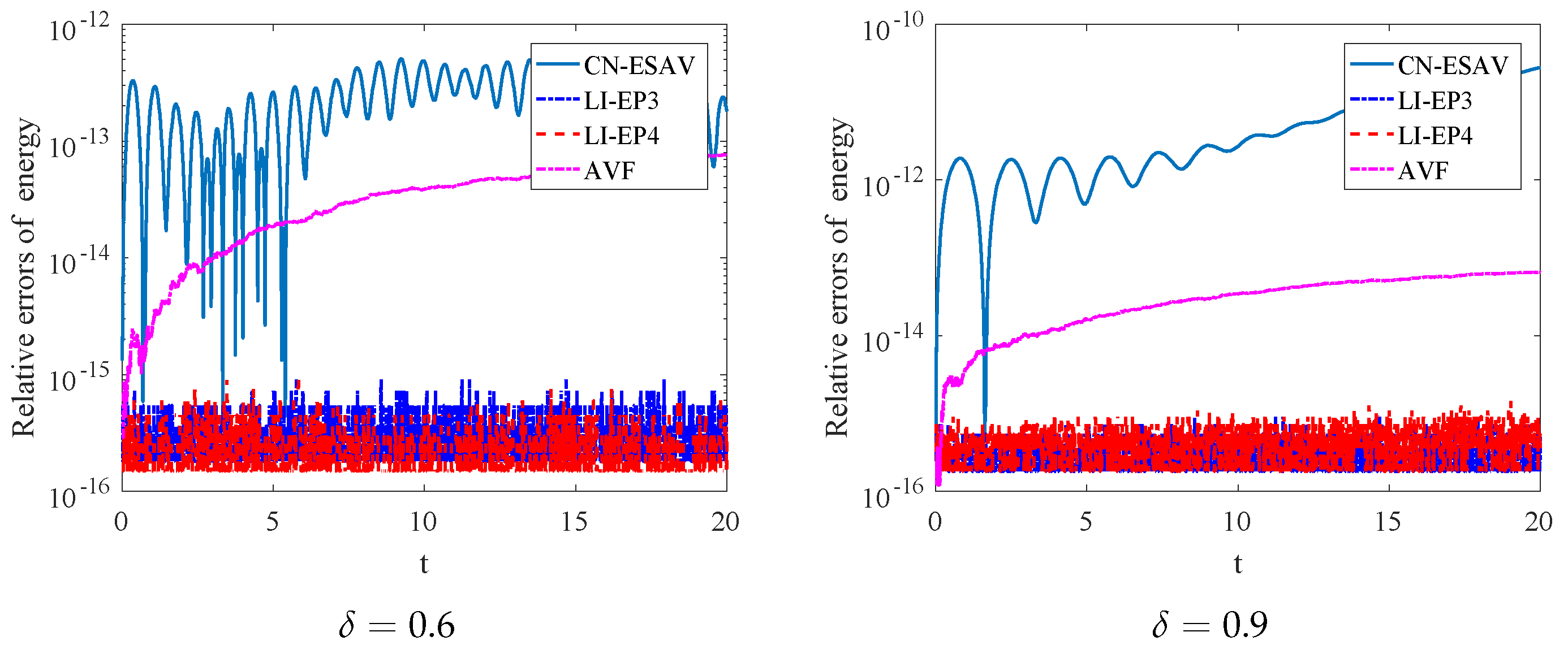
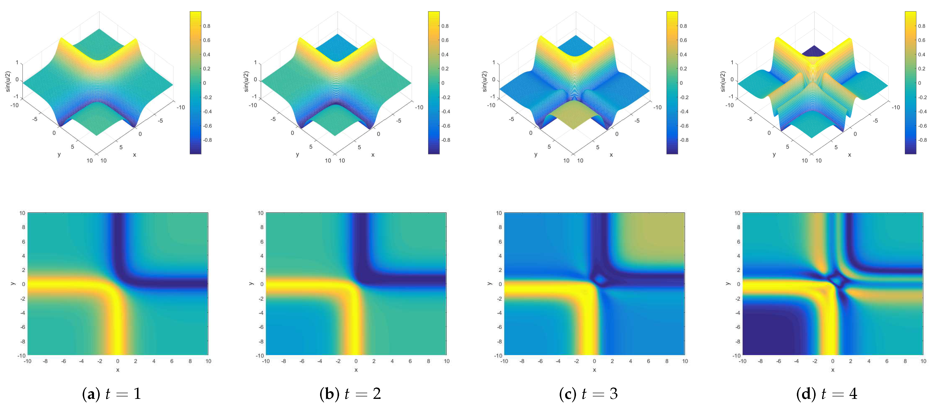
5. Numerical Experiments

This section is dedicated to validating the energy conservation and efficacy of the proposed schemes. We choose $F\left(u\right)=1-\cos \left(u\right)$ and examine nonlocal wave equations under periodic boundary conditions, employing the Fourier pseudo-spectral method for spatial discretization. Additionally, we introduce one method for comparison purposes.

• CN-ESAV: A second-order energy-preserving scheme for the nonlocal wave equation based on the ESAV method.
• AVF: A second-order energy-preserving scheme for the nonlocal wave equation based on the averaged vector field (AVF) method [15].

Example 1. 

This example studies two-dimensional nonlocal wave equation with superposition of two line solitions, the initial conditions are given as follows

$$\begin{array}{cc}\hfill & u(x,y,0)=4\mathrm{atan}(exp(x\left)\right)+\mathrm{atan}(exp(y\left)\right),\hfill \\ \hfill & v(x,y,0)=0,(x,y)\in (-10,10)\times (-10,10).\hfill \end{array}$$

First, we test the accuracy of the constructed linearly implicit schemes. By establishing $h_x=h_y=20/128$ to ensure minimal spatial discretization errors and evaluating the temporal accuracy of the devised three schemes for solving the two-dimensional nonlocal wave system. We compute the numerical errors using the formula ${\parallel e\parallel }_{\infty }={\parallel z(h,\tau )-z(h,\tau /2)\parallel }_{\infty },$ where $z(h,\tau )$ represents the numerical solution at $(h,\tau )$. The provided results, denoted as

Table 1. Errors and corresponding temporal observation orders of the three conservative schemes with different $\delta$ at $t=1$.

$\mathit{\delta }$	$\mathit{\tau }$	CN-ESAV Scheme		LI-EP3  Scheme		LI-EP4  Scheme		AVF Scheme
		${\parallel \mathit{e}\parallel }_{\infty }$	Rate	${\parallel \mathit{e}\parallel }_{\infty }$	Rate	${\parallel \mathit{e}\parallel }_{\infty }$	Rate	${\parallel \mathit{e}\parallel }_{\infty }$	Rate
0.6	0.01	2.0728 × 10−4	-	2.3599 × 10−6	-	3.2338 × 10−7	-	2.8415 × 10−4	-
	0.005	5.3003 × 10−5	1.9674	3.6653 × 10−7	2.6867	2.4979 × 10−8	3.6944	7.2857 × 10−5	1.9635
	0.0025	1.3402 × 10−5	1.9835	5.0776 × 10−8	2.8517	1.7166 × 10−9	3.8631	1.8402 × 10−5	1.9852
0.9	0.01	1.1184 × 10−5	-	7.6434 × 10−8	-	7.8159 × 10−9	-	8.9307 × 10−4	-
	0.005	2.9750 × 10−6	1.9105	1.1263 × 10−8	2.7626	5.7071 × 10−10	3.7756	2.3058 × 10−4	1.9535
	0.0025	7.6704 × 10−7	1.9555	1.5240 × 10−9	2.8857	3.8410 × 10−11	3.8932	5.8709 × 10−5	1.9736

, present the errors in the $L^{\infty }$-norm and their associated convergence rates at $t=1$, where t is the running time. This table demonstrates that all of the schemes proposed in the study yield the anticipated outcomes. Additionally, it is noteworthy that the numerical errors generated by the proposed high accuracy scheme are less than the second-order scheme in the same time step. Figure 1 displays the relative errors of the conservation laws. As shown, three linearly implicit schemes can conserve the modified energy of the system. The interactions of circular vector solitons for component $\sin {\displaystyle \frac{\mathit{u}}{2}}$ with different δ are depicted in Figure 2 and Figure 3. As shown, two expanding ring solitons will collide over time. The rate of these collisions increases with the nonlocal parameter δ, confirming that the nonlocal effect plays a crucial role in the dynamical evolution of the sine-Gordon equation.

Example 2. 

We solve the sine-Gordon equation with collision of two circular solitons by using the proposed schemes, the initial conditions are give by

$$\begin{array}{cc}\hfill & u(x,y,0)=4{tan}^{-1}\left[exp\left({\displaystyle \frac{4-\sqrt{{(x+3)}^2+{(y+7)}^2}}{0.436}}\right)\right],\hfill \\ \hfill & v(x,y,0)={\displaystyle \frac{4.13}{cosh\left(\frac{4-\sqrt{{(x+3)}^2+{(y+7)}^2}}{0.436}\right)}},(x,y)\in (-30,10)\times (-21,7).\hfill \end{array}$$

With τ set to 0.01 and $h_x=h_y$ to 0.1, we plot the deviation of the invariants for the three schemes in Figure 4. The figure indicates that the proposed schemes successfully maintain the modified energy. We also show the evolution of the soliton in Figure 5. The interactions of circular vector solitons for component $\sin {\displaystyle \frac{\mathit{u}}{2}}$ with $\delta =0.8$ are depicted in Figure 5. At $t=0$, $\sin {\displaystyle \frac{\mathit{u}}{2}}$ has two circular solitons that radiate and eventually collide with each other, resulting in unevenness in the central domain. As time passes, the unevenness caused by soliton collisions becomes more pronounced, which precisely verifies that the nonlocal operator significantly impacts the dynamic behavior of the nonlocal wave equation.

6. Conclusions

In this paper, we develop linearly implicit schemes for solving a nonlocal wave equation. The developed schemes are highly accurate and preserve the modified energy. Numerical results also demonstrate their strong numerical stability. Additionally, the methods presented in this study can be applied to other conservative differential equations. In future research, we will address challenges in proving the convergence of these schemes and work on developing efficient conservative schemes that can maintain the original energy of systems.

References

1. Wang, J.; Yang, Z.; Zhang, J. Stability and convergence analysis of high-order numerical schemes with DtN-type absorbing boundary conditions for nonlocal wave equations. IMA J. Numer. Anal. 2023, 44, 1–29. [Google Scholar] [CrossRef]
2. Du, Q.; Ju, L.; Li, X.; Qiao, Z. Stabilized linear semi-implicit schemes for the nonlocal Cahn–Hilliard equation. J. Comput. Phys. 2018, 363, 39–54. [Google Scholar] [CrossRef]
3. Du, Q. Nonlocal Modeling, Analysis, and Computation; SIAM: Philadelphia, PA, USA, 2019. [Google Scholar]
4. Macías-Díaz, J. A structure-preserving method for a class of nonlinear dissipative wave equations with Riesz space-fractional derivatives. J. Comput. Phys. 2017, 351, 40–58. [Google Scholar] [CrossRef]
5. Bates, P.; Brown, S.; Han, J. Numerical analysis for a nonlocal Allen-Cahn equation. Int. J. Numer. Anal. Model. 2009, 6, 33–49. [Google Scholar]
6. Wang, J.; Zhang, J.; Zheng, C. Stability and error analysis for a second-order approximation of 1D nonlocal Schrödinger equation under DtN-typ boundary conditions. Math. Comp. 2023, 334, 761–783. [Google Scholar]
7. Zhao, X.; Sun, Z.; Hao, Z. A fourth-order compact ADI scheme for two-dimensional nonlinear space fractional Schrödinger equation. SIAM. J. Comput. 2014, 36, A2865–A2886. [Google Scholar] [CrossRef]
8. Wang, D.; Xiao, A.; Yang, W. Crank–Nicolson difference scheme for the coupled nonlinear Schrödinger equations with the Riesz space fractional derivative. J. Comput. Phys. 2013, 242, 670–681. [Google Scholar] [CrossRef]
9. Wang, D.; Xiao, A.; Yang, W. A linearly implicit conservative difference scheme for the space fractional coupled nonlinear Schrödinger equations. J. Comput. Phys. 2014, 272, 644–655. [Google Scholar] [CrossRef]
10. Wang, D.; Xiao, A.; Yang, W. Maximum-norm error analysis of a difference scheme for the space fractional CNLS. Appl. Math. Comput. 2015, 257, 241–251. [Google Scholar] [CrossRef]
11. Macías-Díaz, J. A numerically efficient dissipation-preserving implicit method for a nonlinear multidimensional fractional wave equation. J. Sci. Comput. 2018, 77, 1–26. [Google Scholar] [CrossRef]
12. Macías-Díaz, J.; Hendy, A.; Staelen, R. A compact fourth-order in space energy-preserving method for Riesz space-fractional nonlinear wave equations. Appl. Math. Comput. 2018, 325, 1–14. [Google Scholar] [CrossRef]
13. Wang, N.; Li, M.; Huang, C. Unconditional energy dissipation and error estimates of the SAV Fourier spectral method for nonlinear fractional generalized wave equation. J. Sci. Comput. 2021, 88, 19. [Google Scholar] [CrossRef]
14. Li, M.; Fei, M.; Wang, N.; Huang, C. A dissipation-preserving finite element method for nonlinear fractional wave equations on irregular convex domains. Math. Comput. Simul. 2020, 177, 404–419. [Google Scholar] [CrossRef]
15. Cai, W.; Li, H.; Wang, Y. Partitioned averaged vector field methods. J. Comput. Phys. 2018, 370, 25–42. [Google Scholar] [CrossRef]
16. Hu, D.; Cai, W.; Song, Y.; Wang, Y. A fourth-order dissipation-preserving algorithm with fast implementation for space fractional nonlinear damped wave equations. Commun. Nonlinear Sci. Numer. Simul. 2020, 91, 105432. [Google Scholar] [CrossRef]
17. Li, D.; Li, X.; Zhang, Z. Implicit-explicit relaxation Runge-Kutta methods: Construction, analysis and applications to PDEs. Math. Comp. 2023, 339, 92. [Google Scholar] [CrossRef]
18. Brugnano, L.; Zhang, C.; Li, D. A class of energy-conserving Hamiltonian boundary value methods for nonlinear Schrödinger equation with wave operator. Commun. Nonlinear Sci. Numer. Simul. 2018, 60, 33–49. [Google Scholar] [CrossRef]
19. Li, H.; Wang, Y.; Qin, M. A sixth order averaged vector field method. J. Comput. Math. 2016, 34, 479–498. [Google Scholar] [CrossRef]
20. Shen, J.; Xu, J. Convergence and error analysis for the scalar auxiliary variable (SAV) schemes to gradient flows. SIAM J. Numer. Anal. 2018, 56, 2895–2912. [Google Scholar] [CrossRef]
21. Shen, J.; Xu, J.; Yang, J. The scalar auxiliary variable (SAV) approach for gradient flows. J. Comput. Phys. 2018, 353, 407–416. [Google Scholar] [CrossRef]
22. Liu, Z.; Li, X. The exponential scalar auxiliary variable (E-SAV) approach for phase field models and its explicit computing. SIAM J. Sci. Comput. 2020, 42, B630–B655. [Google Scholar] [CrossRef]
23. Hairer, E.; Lubich, C.; Wanner, G. Geometric Numerical Integration: Structure-Preserving Algorithms for Ordinary Differential Equations; Springer Science: Berlin/Heidelberg, Germany, 2006. [Google Scholar]
24. Hu, D.; Kong, L.; Cai, W.; Wang, Y. Fully decoupled, linear and energy-preserving gsav difference schemes for the nonlocal coupled sine-Gordon equations in multiple dimensions. Numer. Algorithms 2023, 95, 1953–1980. [Google Scholar] [CrossRef]
25. Gong, Y.; Zhao, J.; Wang, Q. Arbitrarily high–order linear energy stable schemes for gradient flow models. J. Comput. Phys. 2020, 419, 109610. [Google Scholar] [CrossRef]
26. Li, D.; Sun, W. Linearly implicit and high-order energy-conserving schemes for nonlinear wave equations. J. Sci. Comput. 2020, 83, A3703–A3727. [Google Scholar] [CrossRef]
Figure 1. The relative errors of conservative laws for three schemes with τ = 0.01 , h x = h y = 20 / 128 for different δ .
Mathematics 12 02408 g001
Figure 2. Time evolutions of two-dimensional circular vector solitons for component sin u 2 of a nonlocal wave system with δ = 0.6 . The first row: surface plots; the second row: density plots.
Mathematics 12 02408 g002
Figure 3. Time evolutions of two-dimensional circular vector solitons for component sin u 2 of a nonlocal wave system with δ = 0.9 . The first row: surface plots; the second row: density plots.
Mathematics 12 02408 g003
Figure 4. The relative errors of conservative laws for two schemes with τ = 0.01 , h x = h y = 0.1 .
Mathematics 12 02408 g004
Figure 5. Time evolutions of two-dimensional circular vector solitons for component sin u 2 of nonlocal wave system with δ = 0.8 . The first row: surface plots; the second row: density plots.
Mathematics 12 02408 g005