Research on Stability and Bifurcation for Two-Dimensional Two-Parameter Squared Discrete Dynamical Systems

Abstract

This study investigates a class of two-dimensional, two-parameter squared discrete dynamical systems. It determines the conditions for local stability at the fixed points for these proposed systems. Theoretical and numerical analyses are conducted to examine the bifurcation behavior of the proposed systems. Conditions for the existence of Naimark–Sacker bifurcation, transcritical bifurcation, and flip bifurcation are derived using center manifold theorem and bifurcation theory. Results of the theoretical analyses are validated by numerical simulation studies. Numerical simulations also reveal the complex bifurcation behaviors exhibited by the proposed systems and their advantage in image encryption.

1. Introduction

The bifurcation behavior observed in discrete dynamic systems is fundamentally a nonlinear phenomenon. Bifurcation is relevant across a wide range of fields, including physics, control systems, biology, economics, and chemistry [1,2,3,4]. Numerous real-world phenomena, such as noise generation, aircraft crashes resulting from abrupt wing flapping, predator–prey dynamics in ecology, stock market fluctuations, and the transition of cardiac rhythms from normal beating to fibrillation, can be attributed to bifurcations [5]. Thus, the study of bifurcation in discrete dynamic systems holds substantial theoretical and practical significance.

In recent decades, the bifurcation of discrete dynamic systems has emerged as a prominent area of research among scholars. Initial investigations primarily concentrated on one-dimensional discrete dynamic systems, with logical mapping emerging as the most widely studied example [6]. Despite its simplicity as a mathematical model, this one-dimensional logical mapping exhibits remarkably complex dynamics. Building upon the foundational principles of logical mapping, researchers have subsequently developed new discrete dynamic systems characterized by a diverse array of dynamic behaviors. These behaviors have been found to have practical applications in various fields, including traffic control, cryptography, and image encryption [7]. For instance, reference [8] presented an innovative image encryption method based on logical mapping, while reference [9] proposed a novel model of one-dimensional delay linear coupling logical mapping specifically designed for color image encryption, which demonstrated impressive encryption performance. Moreover, reference [10] introduced a new K-map grounded in logical mapping, which displayed intricate bifurcation and chaotic dynamics, thereby rendering it suitable for applications in traffic control, cryptography, and other related domains.

While one-dimensional discrete dynamic systems exhibit the advantages of a simple structure and ease of implementation, they are characterized by limited sensitivity [11]. In contrast, two-dimensional and higher-dimensional systems better replicate natural conditions compared to their one-dimensional counterparts [12]. By employing central manifold theory, the analysis of high-dimensional systems can be effectively reduced to the analysis of two-dimensional systems [13]. Consequently, a significant body of research has emerged from scholars focusing on the dynamics of two-dimensional discrete dynamic systems. Henon mapping is a two-dimensional dynamical system characterized by a quadratic term, which is notably simplistic in its formulation yet exhibits rich and diverse dynamic behavior [14]. Numerous two-dimensional discrete systems have been developed based on the framework of Henon mapping. For example, reference [15] explored the application of discrete amnesia to Hénon mapping, resulting in an enhanced version characterized by improved chaos and complexity. This adaptation significantly bolsters the performance of the original Hénon mapping and shows promising prospects for practical applications. Reference [16] posited that the improved Hénon mapping can enhance the security of color image encryption algorithms. Additionally, reference [17] introduced a new discrete simplified Lorentz map, also incorporating a quadratic term, which elucidates the occurrence of bifurcations and chaotic behavior while simultaneously mitigating the complexities associated with the traditional Lorentz map. Collectively, these studies underscore the intricate dynamic behaviors inherent in discrete dynamical systems featuring quadratic terms.

The existing literature indicates that a novel type of discrete dynamic system can be developed through the deformation and coupling of two one-dimensional discrete dynamic systems [18]. Reference [19] explored the bifurcation behavior associated with fixed points in linear coupled logical systems. Reference [20] presented a two-dimensional noninvertible mapping that integrates linear mapping with a nonlinear cubic term. The authors derive the conditions for the existence of various bifurcations, including pitchfork bifurcation, flip bifurcation, and Naimark–Sacker bifurcation, utilizing the central manifold theorem alongside bifurcation theory in [20]. Reference [21] constructed two-dimensional parabolic discrete mapping through the nonlinear coupling of one-dimensional logical mapping and square mapping. Furthermore, reference [22] investigated the coupling system of two logical mappings. Collectively, these findings demonstrate that nonlinear coupling mapping significantly alters the dynamic characteristics of discrete systems, leading to the emergence of nonlinear physical phenomena such as bifurcations [23]. Building upon the advantages of logical mapping and discrete mapping that includes square terms, this paper proposes a two-dimensional, two-parameter discrete dynamic system characterized by a square term. The dynamic behavior of this proposed system is analyzed both theoretically and numerically.

This paper is organized as follows. In Section 2, a class of two-dimensional two-parameter squared discrete dynamical systems are constructed, and the fixed points for these proposed systems are computed. Subsequently, the stability of the fixed points is analyzed, and the local stability conditions at these points are discussed. In Section 3, theoretical analysis is conducted on the bifurcation behaviors of the proposed systems. The conditions for the existence of Naimark–Sacker bifurcations, transcritical bifurcations, and flip bifurcations are obtained. In Section 4, the numerical simulations are carried out. The numerical analysis is used to verify the validity of the theoretical analysis. In Section 5, the main conclusions of the work are summarized.

2. Existence and Stability of Fixed Points

In this paper, we consider a class of two-dimensional two-parameter squared discrete dynamical systems, which take the form

$$F:\left\{\begin{array}{l}x\mapsto ax+{\displaystyle \frac{3}{2}}y\\ y\mapsto b(x-x^2)\end{array}\right.$$

(1)

where $a\ne 0,b\ne 0$.

2.1. Existence of Fixed Points

Let $P\left(x_0,y_0\right)$ be the fixed point of the two-dimensional two-parameter squared discrete dynamical system (1); then, the point satisfies the equation

$$\left\{\begin{array}{c}{x}_0=a{x}_0+{\displaystyle \frac{3}{2}}{y}_0\\ y_0=b\left(x_0-x_0^2\right)\end{array}\right.$$

(2)

and the Jacobi matrix of the discrete dynamical system (1) at the fixed point $P\left(x_0,y_0\right)$ is

$$DF(x_0,y_0)=\left[\begin{array}{cc}a& {\displaystyle \frac{3}{2}}\\ b-2b{x}_0& 0\end{array}\right]$$

Its characteristic equation is ${\lambda }^2-a\lambda +3b{x}_0-{\displaystyle \frac{3}{2}}b=0$.

By a simple calculation, we can obtain the following proposition:

Proposition 1.

When $x_0=0$, the fixed point of the discrete dynamical system (1) is $P_1\left(0,0\right)$; when $x_0\ne 0$, the fixed point of the discrete dynamical system (1) is $P_2\left({\displaystyle \frac{2a}{3b}}+1-{\displaystyle \frac{2}{3b}},{\displaystyle \frac{2}{3}}\left(1-a\right)\left({\displaystyle \frac{2a}{3b}}+1-{\displaystyle \frac{2}{3b}}\right)\right)$.

2.2. Stability at the Fixed Point $P_1\left(0,0\right)$

For investigating the stability at the fixed point $P_1\left(0,0\right)$ of the discrete dynamical system (1), we calculate the Jacobian matrix at the fixed point $P_1\left(0,0\right)$. The Jacobian matrix at the fixed point $P_1\left(0,0\right)$ is given by $DF(0,0)=\left[\begin{array}{cc}a& {\displaystyle \frac{3}{2}}\\ b& 0\end{array}\right]$. Its characteristic equation is ${\lambda }^2-a\lambda -{\displaystyle \frac{3}{2}}b=0$, and the eigenvalues are given by ${\lambda }_1={\displaystyle \frac{a+\sqrt{a^2+6b}}{2}}$ and ${\lambda }_2={\displaystyle \frac{a-\sqrt{a^2+6b}}{2}}$.

Theorem 1.

For the two-dimensional two-parameter squared discrete dynamical system (1), the stability at the fixed point $P_1\left(0,0\right)$ is listed as follows:

(1) 

When $a^2+6b=0$:

If $a=\pm 2$, $b=-{\displaystyle \frac{2}{3}}$, $P_1\left(0,0\right)$ is a critical node; if $-2<a<2$, $b=-{\displaystyle \frac{a^2}{6}}$, $P_1\left(0,0\right)$ is a stable node; if $a>2$ or $a<-2$, $b=-{\displaystyle \frac{a^2}{6}}$, $P_1\left(0,0\right)$ is an unstable node.

(2) 

When $a^2+6b<0$:

If $b<-{\displaystyle \frac{2}{3}}$, $P_1\left(0,0\right)$ is an unstable focus; if $-{\displaystyle \frac{2}{3}}<b<0$, $P_1\left(0,0\right)$ is a stable focus.

(3) 

When $a^2+6b>0$:

If $a>0$, $b>{\displaystyle \frac{2}{3}}\left(1+a\right)$, $P_1\left(0,0\right)$ is an unstable node; if $a>0$, ${\displaystyle \frac{2}{3}}\left(1-a\right)<b<{\displaystyle \frac{2}{3}}\left(1+a\right)$, $P_1\left(0,0\right)$ is a saddle; if $a>2$, $b<{\displaystyle \frac{2}{3}}\left(1-a\right)$, $P_1\left(0,0\right)$ is an unstable node; if $0<a<2$, $b<{\displaystyle \frac{2}{3}}\left(1-a\right)$, $P_1\left(0,0\right)$ is a stable node.

If $a<0$, $b>{\displaystyle \frac{2}{3}}\left(1-a\right)$, $P_1\left(0,0\right)$ is an unstable node; if $a<0$, ${\displaystyle \frac{2}{3}}\left(1+a\right)<b<{\displaystyle \frac{2}{3}}\left(1-a\right)$, $P_1\left(0,0\right)$ is a saddle; if $-2<a<0$, $b<{\displaystyle \frac{2}{3}}\left(1+a\right)$, $P_1\left(0,0\right)$ is a stable node; if $a<-2$, $b<{\displaystyle \frac{2}{3}}\left(1+a\right)$, $P_1\left(0,0\right)$ is an unstable node.

Proof. 

(1) When $a^2+6b=0$, the eigenvalue $\left|{\lambda }_1\right|=\left|{\lambda }_2\right|={\displaystyle \frac{\left|a\right|}{2}}$. If ${\displaystyle \frac{\left|a\right|}{2}}=1$, then $a=\pm 2$, $b=-{\displaystyle \frac{2}{3}}$, $P_1\left(0,0\right)$ is a critical node. When $-2<a<2$, $\left|{\lambda }_1\right|=\left|{\lambda }_2\right|={\displaystyle \frac{\left|a\right|}{2}}<1$, then the fixed point $P_1\left(0,0\right)$ is a stable node; when $a>2$ or $a<-2$, $\left|{\lambda }_1\right|=\left|{\lambda }_2\right|={\displaystyle \frac{\left|a\right|}{2}}>1$, then the fixed point $P_1\left(0,0\right)$ is an unstable node.

(2) When $a^2+6b<0$, eigenvalues ${\lambda }_1={\displaystyle \frac{a+i\sqrt{-a^2-6b}}{2}}$ and ${\lambda }_2={\displaystyle \frac{a-i\sqrt{-a^2-6b}}{2}}$ are two conjugate complex numbers. They are equivalent to ${\lambda }_1=\sqrt{-{\displaystyle \frac{3}{2}}b}{e}^{i\arctan {\displaystyle \frac{\sqrt{-a^2-6b}}{a}}}$ and ${\lambda }_2=\sqrt{-{\displaystyle \frac{3}{2}}b}{e}^{-i\arctan {\displaystyle \frac{\sqrt{-a^2-6b}}{a}}}$. When $b=-{\displaystyle \frac{2}{3}}$, $\left|{\lambda }_1\right|=\left|{\lambda }_2\right|=1$, and $a^2+6b<0$, then $-2<a<2$. When $b<-{\displaystyle \frac{2}{3}}$, $\left|{\lambda }_1\right|=\left|{\lambda }_2\right|>1$, then the fixed point $P_1\left(0,0\right)$ is an unstable focus; when $-{\displaystyle \frac{2}{3}}<b<0$, $\left|{\lambda }_1\right|=\left|{\lambda }_2\right|<1$, then the fixed point $P_1\left(0,0\right)$ is a stable focus.

(3) When $a^2+6b>0$, the eigenvalues ${\lambda }_1, {\lambda }_2$ are two real numbers. It is obviously ${\lambda }_1>{\lambda }_2$. A discussion is as follows:

① It is supposed that ${\lambda }_1>{\lambda }_2>1$. Since ${\lambda }_1>{\lambda }_2$, it only needs to satisfy ${\lambda }_2={\displaystyle \frac{a-\sqrt{a^2+6b}}{2}}>1$. It is equivalent to $b<{\displaystyle \frac{2}{3}}\left(1-a\right)$ and $a-2>0$. Thus, if $a>2$ and $b<{\displaystyle \frac{2}{3}}\left(1-a\right)$, the fixed point $P_1\left(0,0\right)$ is an unstable node.

② It is supposed that ${\lambda }_2<{\lambda }_1<-1$. Since ${\lambda }_1>{\lambda }_2$, it only needs to satisfy ${\lambda }_1={\displaystyle \frac{a+\sqrt{a^2+6b}}{2}}<-1$. It is equivalent to $-2-a>0$ and $b<{\displaystyle \frac{2}{3}}\left(1+a\right)$. Thus, if $a<-2$ and $b<{\displaystyle \frac{2}{3}}\left(1+a\right)$, the fixed point $P_1\left(0,0\right)$ is an unstable node.

③ It is supposed that ${\lambda }_2<-1$ and ${\lambda }_1>1$. Since ${\displaystyle \frac{a+\sqrt{a^2+6b}}{2}}>1$ and ${\displaystyle \frac{a-\sqrt{a^2+6b}}{2}}<-1$, so $\sqrt{a^2+6b}>2-a$ and $\sqrt{a^2+6b}>2+a$. It is equivalent to $a>0$, $b>{\displaystyle \frac{2}{3}}\left(1+a\right)$ and $a<0$, $b>{\displaystyle \frac{2}{3}}\left(1-a\right)$. Thus, if $a>0$, $b>{\displaystyle \frac{2}{3}}\left(1+a\right)$, the fixed point $P_1\left(0,0\right)$ is an unstable node; if $a<0$, $b>{\displaystyle \frac{2}{3}}\left(1-a\right)$, the fixed point $P_1\left(0,0\right)$ is also an unstable node.

④ It is supposed that $-1<{\lambda }_2<{\lambda }_1<1$. It only needs to satisfy ${\displaystyle \frac{a+\sqrt{a^2+6b}}{2}}<1$ and ${\displaystyle \frac{a-\sqrt{a^2+6b}}{2}}>-1$. Under a simple calculation, it is equivalent to $0<a<2$, $b<{\displaystyle \frac{2}{3}}\left(1-a\right)$ and $-2<a<0$, $b<{\displaystyle \frac{2}{3}}\left(1+a\right)$. Thus, if $0<a<2$, $b<{\displaystyle \frac{2}{3}}\left(1-a\right)$, the fixed point $P_1\left(0,0\right)$ is a stable node; if $-2<a<0$, $b<{\displaystyle \frac{2}{3}}\left(1+a\right)$, the fixed point $P_1\left(0,0\right)$ is also a stable node.

⑤ It is supposed that ${\lambda }_2<-1,-1<{\lambda }_1<1$. Since ${\displaystyle \frac{a-\sqrt{a^2+6b}}{2}}<-1$ and $-1<{\displaystyle \frac{a+\sqrt{a^2+6b}}{2}}<1$, a simple calculation can decide $a<0$, ${\displaystyle \frac{2}{3}}\left(1+a\right)<b<{\displaystyle \frac{2}{3}}\left(1-a\right)$. Thus, if $a<0$,${\displaystyle \frac{2}{3}}\left(1+a\right)<b<{\displaystyle \frac{2}{3}}\left(1-a\right)$, the fixed point $P_1\left(0,0\right)$ is a saddle.

⑥ It is supposed that $-1<{\lambda }_2<1,{\lambda }_1>1$. Since $-1<{\displaystyle \frac{a-\sqrt{a^2+6b}}{2}}<1$ and ${\displaystyle \frac{a+\sqrt{a^2+6b}}{2}}>1$, a simple calculation can decide $a>0$, ${\displaystyle \frac{2}{3}}\left(1-a\right)<b<{\displaystyle \frac{2}{3}}\left(1+a\right)$. Thus, if $a>0$, ${\displaystyle \frac{2}{3}}\left(1-a\right)<b<{\displaystyle \frac{2}{3}}\left(1+a\right)$, the fixed point $P_1\left(0,0\right)$ is a saddle. □

2.3. Stability at the Nonzero Fixed Point $P_2\left({\displaystyle \frac{2a}{3b}}+1-{\displaystyle \frac{2}{3b}},{\displaystyle \frac{2}{3}}\left(1-a\right)\left({\displaystyle \frac{2a}{3b}}+1-{\displaystyle \frac{2}{3b}}\right)\right)$

For investigating the stability at the nonzero fixed point of the discrete dynamical system (1), we calculate the Jacobian matrix at the nonzero fixed point $P_2\left({\displaystyle \frac{2a}{3b}}+1-{\displaystyle \frac{2}{3b}},{\displaystyle \frac{2}{3}}\left(1-a\right)\left({\displaystyle \frac{2a}{3b}}+1-{\displaystyle \frac{2}{3b}}\right)\right)$. The Jacobian matrix at the fixed point $P_2\left({\displaystyle \frac{2a}{3b}}+1-{\displaystyle \frac{2}{3b}},{\displaystyle \frac{2}{3}}\left(1-a\right)\left({\displaystyle \frac{2a}{3b}}+1-{\displaystyle \frac{2}{3b}}\right)\right)$ is given by

$$DF\left({\displaystyle \frac{2a}{3b}}+1-{\displaystyle \frac{2}{3b}},{\displaystyle \frac{2}{3}}\left(1-a\right)\left({\displaystyle \frac{2a}{3b}}+1-{\displaystyle \frac{2}{3b}}\right)\right)=\left[\begin{array}{cc}a& {\displaystyle \frac{3}{2}}\\ -{\displaystyle \frac{4a}{3}}-b+{\displaystyle \frac{4}{3}}& 0\end{array}\right]$$

Its characteristic equation is ${\lambda }^2-a\lambda +2a+{\displaystyle \frac{3}{2}}b-2=0$, and the eigenvalues are given by ${\lambda }_1={\displaystyle \frac{a+\sqrt{a^2-8a-6b+8}}{2}}$ and ${\lambda }_2={\displaystyle \frac{a-\sqrt{a^2-8a-6b+8}}{2}}$.

Theorem 2.

For the two-dimensional two-parameter squared discrete dynamical system (1), stability at the nonzero fixed point $P_2$ is listed as follows:

(1) 

When $a^2-8a-6b+8=0$:

If $a=2$, $b=-{\displaystyle \frac{2}{3}}$, $P_2$ is a critical node; if $a=-2$, $b={\displaystyle \frac{14}{3}}$, $P_2$ is a critical node.

If $-2<a<2$, $b={\displaystyle \frac{a^2-8a+8}{6}}$, $P_2$ is a stable node; if $a<-2$ or $a>2$, $b={\displaystyle \frac{a^2-8a+8}{6}}$, $P_2$ is an unstable node.

(2) 

When $a^2-8a-6b+8<0$:

If ${\displaystyle \frac{4}{3}}-{\displaystyle \frac{4a}{3}}<b<2-{\displaystyle \frac{4a}{3}}$, $P_2$ is a stable focus; if $b>2-{\displaystyle \frac{4a}{3}}$, $P_2$ is an unstable focus.

(3) 

When $a^2-8a-6b+8>0$:

If $a>0$, $b<{\displaystyle \frac{2}{3}}-2a$, $P_2$ is an unstable node; if $a>0$, ${\displaystyle \frac{2}{3}}-2a<b<{\displaystyle \frac{2}{3}}(1-a)$, $P_2$ is a saddle; if $0<a<2$, $b>{\displaystyle \frac{2}{3}}(1-a)$, $P_2$ is a stable node; if $a>2$, $b>{\displaystyle \frac{2}{3}}(1-a)$, $P_2$ is an unstable node.

If $a<0$, $b<{\displaystyle \frac{2}{3}}(1-a)$, $P_2$ is an unstable node; if $a<0$, ${\displaystyle \frac{2}{3}}(1-a)<b<{\displaystyle \frac{2}{3}}-2a$, $P_2$ is a saddle; if $-2<a<0$, $b>{\displaystyle \frac{2}{3}}-2a$, $P_2$ is a stable node; if $a<-2$, $b>{\displaystyle \frac{2}{3}}-2a$, $P_2$ is an unstable node.

Proof. 

(1) When $a^2-8a-6b+8=0$, ${\lambda }_1={\lambda }_2={\displaystyle \frac{a}{2}}$. If $a=\pm 2$, ${\lambda }_1={\lambda }_2=\pm 1$, thus $P_2$ is a critical node. If $-2<a<2$, then $-1<{\lambda }_1={\lambda }_2<1$, the fixed point $P_2$ is a stable node; if $a<-2$ or $a>2$, then $\left|{\lambda }_1\right|=\left|{\lambda }_2\right|>1$, the fixed point $P_2$ is an unstable node.

(2) When $a^2-8a-6b+8<0$, ${\lambda }_1={\displaystyle \frac{a+i\sqrt{-a^2+8a+6b-8}}{2}}$ and ${\lambda }_2={\displaystyle \frac{a-i\sqrt{-a^2+8a+6b-8}}{2}}$ are a pair of conjugate complex numbers, which are equivalent to

$${\lambda }_1=\sqrt{{\displaystyle \frac{8a+6b-8}{4}}}{e}^{i\arctan {\displaystyle \frac{\sqrt{-a^2+8a+6b-8}}{a}}},{\lambda }_2=\sqrt{{\displaystyle \frac{8a+6b-8}{4}}}{e}^{-i\arctan {\displaystyle \frac{\sqrt{-a^2+8a+6b-8}}{a}}}.$$

If $\left|{\lambda }_1\right|=\left|{\lambda }_2\right|=1$, $b=2-{\displaystyle \frac{4a}{3}}$. Meanwhile, $a^2-8a-6b+8<0$, we can deduce $-2<a<2$. When ${\displaystyle \frac{4}{3}}-{\displaystyle \frac{4a}{3}}<b<2-{\displaystyle \frac{4a}{3}}$, $\left|{\lambda }_1\right|=\left|{\lambda }_2\right|<1$, thus $P_2$ is a stable focus; when $b>2-{\displaystyle \frac{4a}{3}}$, $\left|{\lambda }_1\right|=\left|{\lambda }_2\right|>1$, thus $P_2$ is an unstable focus.

(3) When $a^2-8a-6b+8>0$, ${\lambda }_1={\displaystyle \frac{a+\sqrt{a^2-8a-6b+8}}{2}}$ and ${\lambda }_2={\displaystyle \frac{a-\sqrt{a^2-8a-6b+8}}{2}}$ are two real numbers. It is clearly ${\lambda }_1>{\lambda }_2$, with discussions as follows:

① It is supposed that ${\lambda }_1>{\lambda }_2>1$. Since ${\lambda }_1>{\lambda }_2$, it only needs to satisfy ${\lambda }_2={\displaystyle \frac{a-\sqrt{a^2-8a-6b+8}}{2}}>1$. It is equivalent to $b>{\displaystyle \frac{2}{3}}-{\displaystyle \frac{2a}{3}}$ and $a-2>0$. Thus, if $a>2$ and $b>{\displaystyle \frac{2}{3}}-{\displaystyle \frac{2a}{3}}$, the fixed point $P_2$ is an unstable node.

② It is supposed that ${\lambda }_2<{\lambda }_1<-1$. It only needs ${\lambda }_1={\displaystyle \frac{a+\sqrt{a^2-8a-6b+8}}{2}}<-1$. A simple calculation can deduce $b>{\displaystyle \frac{2}{3}}-2a$ and $-2-a>0$. Thus, if $a<-2$, $b>{\displaystyle \frac{2}{3}}-2a$, the fixed point $P_2$ is an unstable node.

③ It is supposed that ${\lambda }_1>1$ and ${\lambda }_2<-1$. Since ${\displaystyle \frac{a+\sqrt{a^2-8a-6b+8}}{2}}>1$ and ${\displaystyle \frac{a-\sqrt{a^2-8a-6b+8}}{2}}<-1$, we can deduce $a>0$, $b<{\displaystyle \frac{2}{3}}-2a$. Thus, if $a<0$, $b<{\displaystyle \frac{2}{3}}(1-a)$, the fixed point $P_2$ is an unstable node.

④ It is supposed that $-1<{\lambda }_2<{\lambda }_1<1$. Since ${\displaystyle \frac{a+\sqrt{a^2-8a-6b+8}}{2}}<1$ and ${\displaystyle \frac{a-\sqrt{a^2-8a-6b+8}}{2}}>-1$, we can deduce that if $-2<a<0$, then $b>{\displaystyle \frac{2}{3}}-2a$, the fixed point $P_2$ is a stable node. If $0<a<2$, then $b>{\displaystyle \frac{2}{3}}(1-a)$, the fixed point $P_2$ is a stable node.

⑤ It is supposed that ${\lambda }_1>1$, $-1<{\lambda }_2<1$. Since ${\displaystyle \frac{a+\sqrt{a^2-8a-6b+8}}{2}}>1$ and $-1<{\displaystyle \frac{a-\sqrt{a^2-8a-6b+8}}{2}}<1$, it can deduce $a>0$, ${\displaystyle \frac{2}{3}}-2a<b<{\displaystyle \frac{2}{3}}-{\displaystyle \frac{2a}{3}}$. Thus, if $a>0$, ${\displaystyle \frac{2}{3}}-2a<b<{\displaystyle \frac{2}{3}}-{\displaystyle \frac{2a}{3}}$, the fixed point $P_2$ is a saddle.

⑥ It is supposed that $-1<{\lambda }_1<1$ and ${\lambda }_2<-1$. Since $-1<{\displaystyle \frac{a+\sqrt{a^2-8a-6b+8}}{2}}<1$, ${\displaystyle \frac{a-\sqrt{a^2-8a-6b+8}}{2}}<-1$, we can deduce that $a<0$, ${\displaystyle \frac{2}{3}}(1-a)<b<{\displaystyle \frac{2}{3}}-2a$. Thus, if $a<0$, ${\displaystyle \frac{2}{3}}(1-a)<b<{\displaystyle \frac{2}{3}}-2a$, the fixed point $P_2$ is a saddle. □

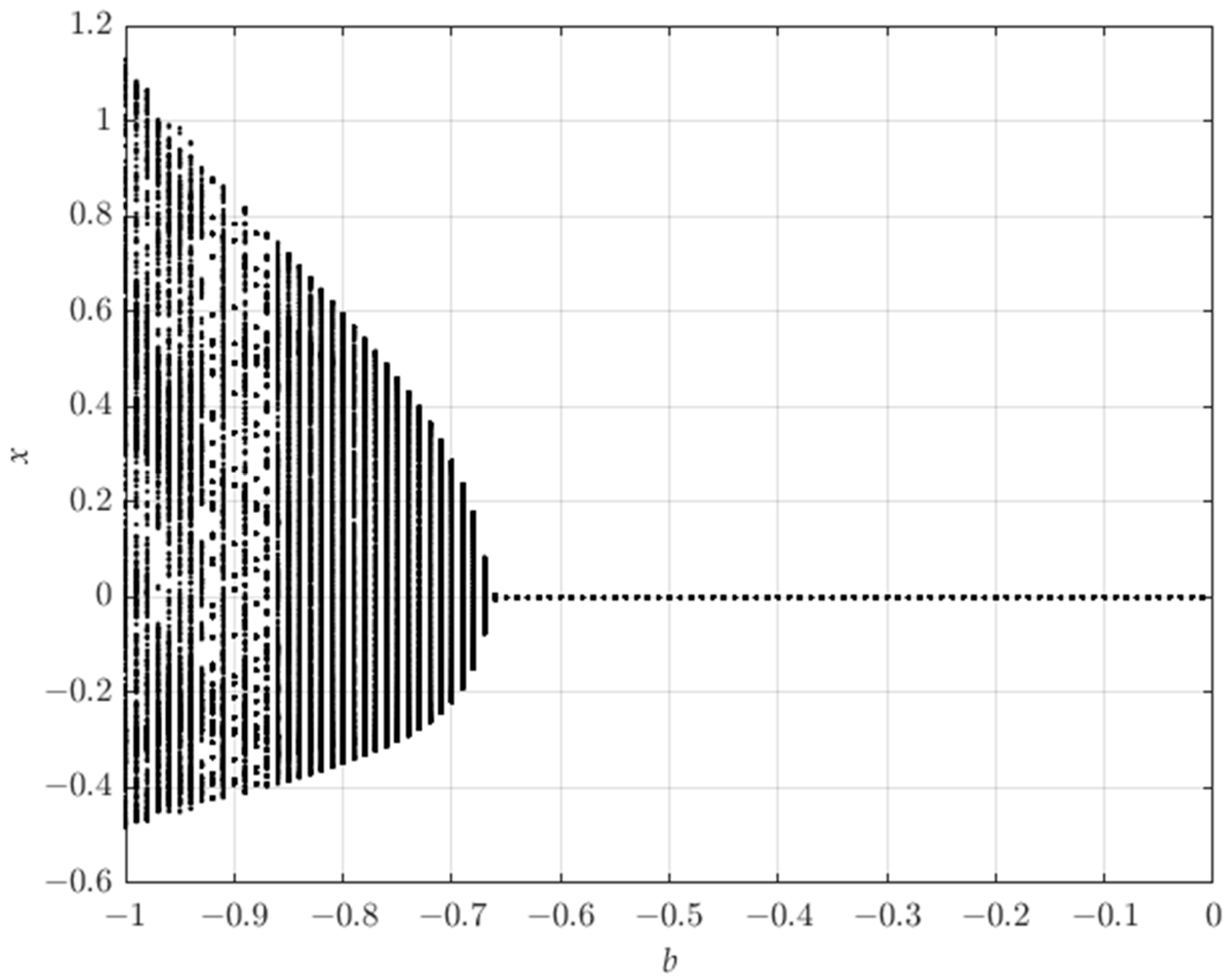
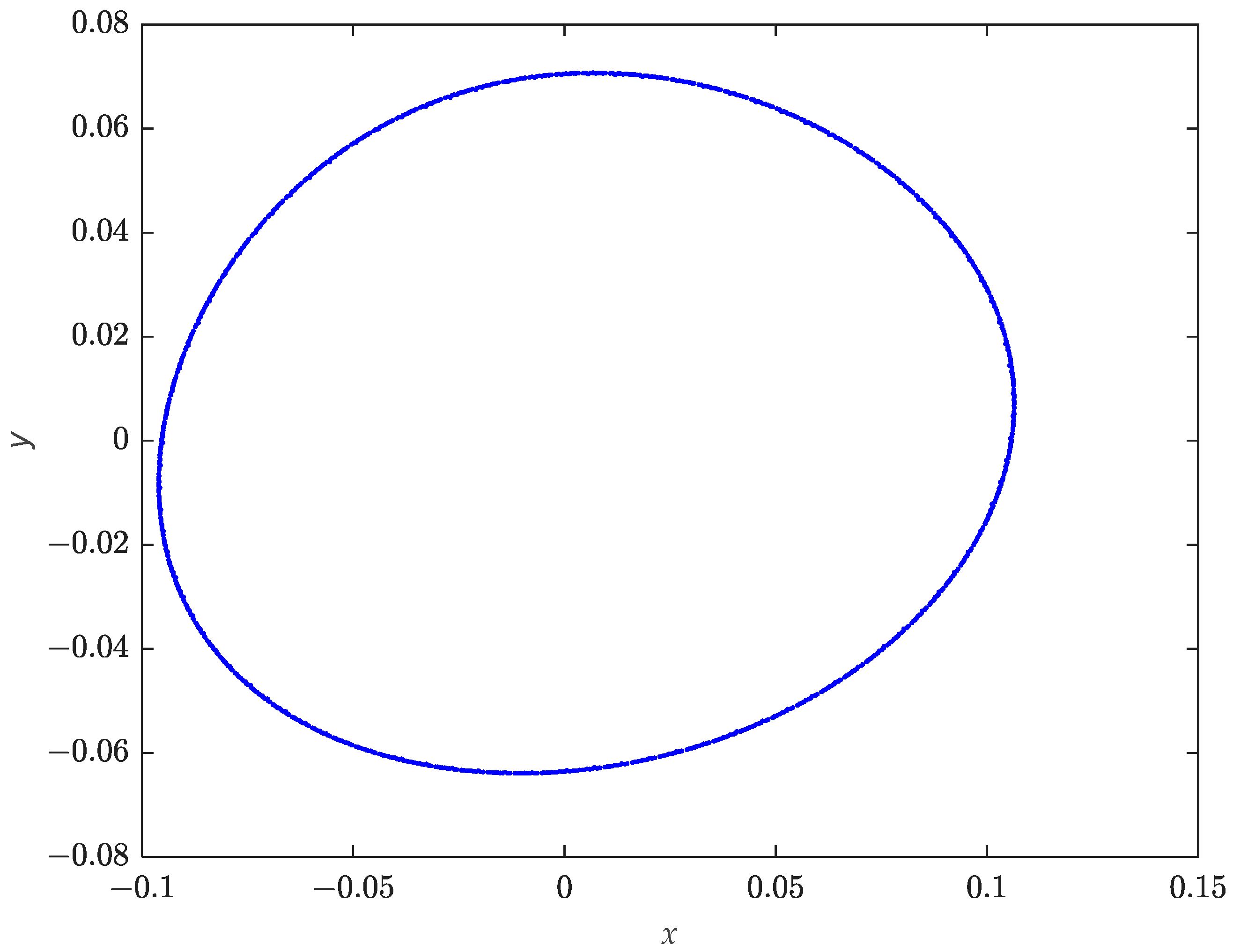
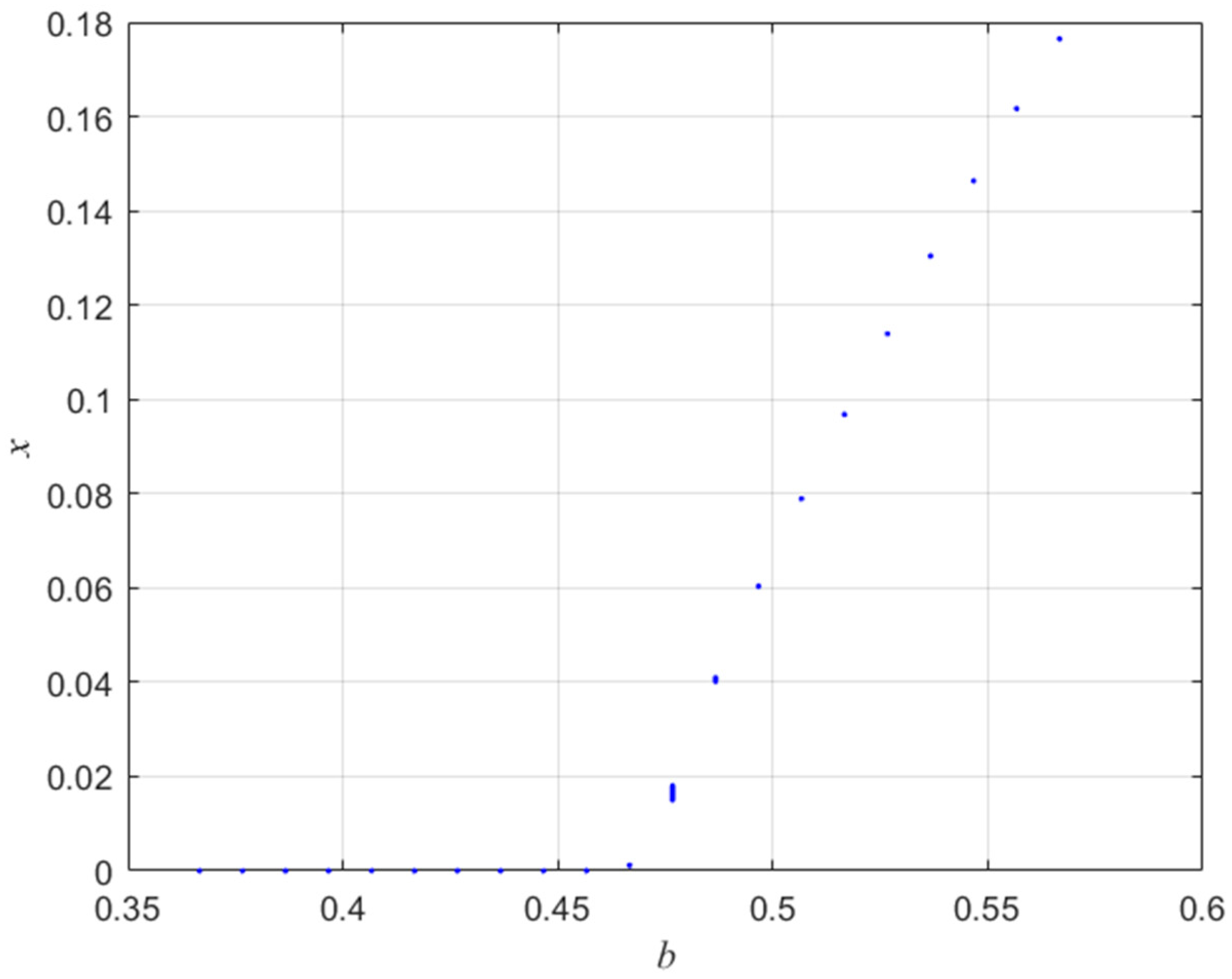
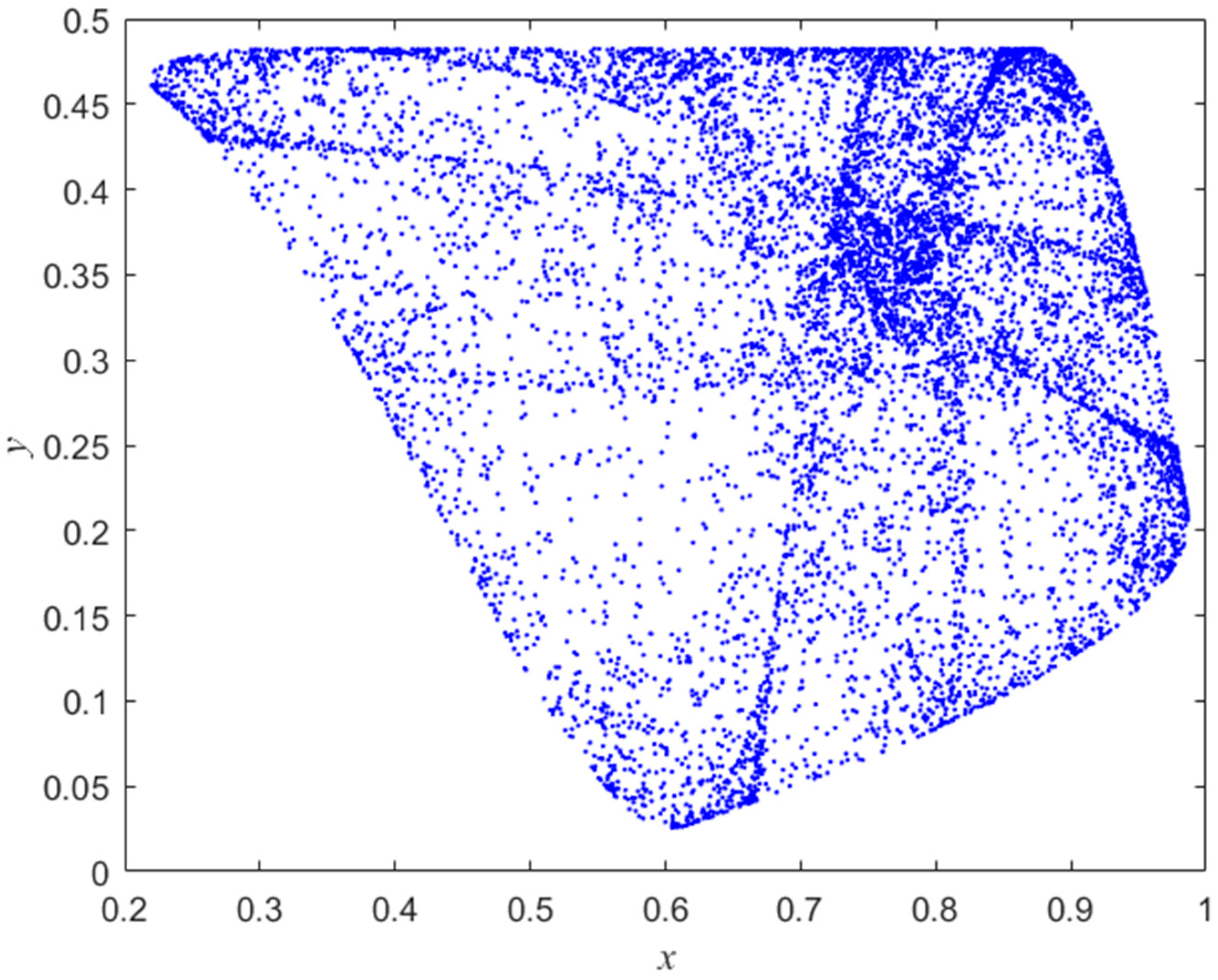
3. Bifurcation Analysis

With the discussion of Section 2.2, it can be found that the stability at $P_1\left(0,0\right)$ can be changed at $\mathrm{b}=-{\displaystyle \frac{2}{3}}$, $\mathrm{b}={\displaystyle \frac{2}{3}}\left(1-a\right)$ and $\mathrm{b}={\displaystyle \frac{2}{3}}\left(1+a\right)$. Therefore, we will study the bifurcations at the fixed point $P_1\left(0,0\right)$ for $\mathrm{b}=-{\displaystyle \frac{2}{3}}$, $\mathrm{b}={\displaystyle \frac{2}{3}}\left(1-a\right)$ and $\mathrm{b}={\displaystyle \frac{2}{3}}\left(1+a\right)$ in this section.

Lemma 1.

(Naimark–Sacker Bifurcation Existence Theorem for Discrete Dynamical Systems [24]): Let $f_{\mu }:{\mathbb{R}}^2\mapsto {\mathbb{R}}^2$ be a one-parameter family of mappings which has a smooth family of fixed points $x(\mu )$ at which the eigenvalues are complex conjugates $\lambda (\mu )$, $\overline{\lambda }(\mu )$. Assume

(SH1) $\left|\lambda ({\mu }_0)\right|=1$, but ${\lambda }^j({\mu }_0)\ne 1$ for $j=1,2,3,4$.

(SH2) ${\displaystyle \frac{d}{d\mu }}(\left|\lambda ({\mu }_0)\right|)=d\ne 0$.

Then, there is a smooth change in coordinates $h$ so that the expression of $h{f}_{\mu }{h}^{-1}$ in polar coordinates has the form

$$h{f}_{\mu }{h}^{-1}(r,\theta )=(r(1+d(\mu -{\mu }_0)+a{r}^2,\theta +c+b{r}^2)+\mathrm{higher}-\mathrm{order} \mathrm{terms}$$

(Note: $\lambda$ complex and (SH2) imply $\left|\arg (\lambda )\right|=c$ and $d$ are nonzero).

If, in addition

(SH3) $a\ne 0$.

Then, there is a two-dimensional surface $\mathrm{\Sigma }$ (not necessarily infinitely differentiable) in ${\mathbb{R}}^2\times \mathbb{R}$ having quadratic tangency with the plane ${\mathbb{R}}^2\times \left\{{\mu }_0\right\}$ which is invariant for $f_{\mu }$. If $\mathrm{\Sigma }\cap ({\mathbb{R}}^2\times \{\mu \})$ is larger than a point, then it is a simple closed curve.

Assume that the bifurcating system (restricted to the center manifold) is in the form

$$\left(\begin{array}{c}x\\ y\end{array}\right)\mapsto \left[\begin{array}{cc}\cos (c)& -\sin (c)\\ \sin (c)& \cos (c)\end{array}\right]\left(\begin{array}{c}x\\ y\end{array}\right)+\left(\begin{array}{c}f(x,y)\\ g(x,y)\end{array}\right)$$

With eigenvalues $\lambda ,\overline{\lambda }=e^{\pm ic}$, one obtains

$$a=-\mathrm{Re}\left[{\displaystyle \frac{(1-2\lambda ){\overline{\lambda }}^2}{1-\lambda }}{\xi }_{11}{\xi }_{20}\right]-{\displaystyle \frac{1}{2}}{\left|{\xi }_{11}\right|}^2-{\left|{\xi }_{02}\right|}^2+\mathrm{Re}(\overline{\lambda }{\xi }_{21})$$

where

$${\xi }_{20}={\displaystyle \frac{1}{8}}\left[(f_{xx}-f_{yy}+2g_{xy})+i(g_{xx}-g_{yy}-2f_{xy})\right]$$

$${\xi }_{11}={\displaystyle \frac{1}{4}}\left[(f_{xx}+f_{yy})+i(g_{xx}+g_{yy})\right]$$

$${\xi }_{02}={\displaystyle \frac{1}{8}}\left[(f_{xx}-f_{yy}-2g_{xy})+i(g_{xx}-g_{yy}+2f_{xy})\right]$$

$${\xi }_{21}={\displaystyle \frac{1}{16}}\left[(f_{xxx}+f_{xyy}+g_{xxy}+g_{yyy})+i(g_{xxx}+g_{xyy}-f_{xxy}-f_{yyy})\right]$$

Theorem 3.

If $-2<a<2$ and $a\ne -1$, 0, the two-dimensional two-parameter squared discrete dynamical system (1) has a Naimark–Sacker bifurcation at the fixed point $P_1\left(0,0\right)$ for $b=-{\displaystyle \frac{2}{3}}$.

Proof. 

For the two-dimensional two-parameter squared discrete dynamical system (1), it is assumed that the Jacobian matrix at the fixed point $P_1\left(0,0\right)$ has a pair of conjugate complex eigenvalues $\lambda ={\displaystyle \frac{a+\sqrt{a^2+6b}}{2}}$ and $\overline{\lambda }={\displaystyle \frac{a-\sqrt{a^2+6b}}{2}}$.

To ensure that $\left|\lambda \left(b\right)\right|=\sqrt{{\displaystyle \frac{a^2}{4}}+{\displaystyle \frac{\left(-a^2-6b\right)}{4}}}=\sqrt{-{\displaystyle \frac{3b}{2}}}=1$, it only needs $-{\displaystyle \frac{3b}{2}}=1$, i.e., $b=-{\displaystyle \frac{2}{3}}$. Let $\Delta =a^2+6b<0$; it can deduce that $b<-{\displaystyle \frac{a^2}{6}}$ and $-2<a<2$.

After a simple calculation, we can derive that if $a\ne -1,0$, then ${\left[\lambda \left(-{\displaystyle \frac{2}{3}}\right)\right]}^n\ne 1$, where $n=1,2,3,4$. And ${\displaystyle \frac{d}{d\left(b\right)}}\left(\left|\lambda \left(-{\displaystyle \frac{2}{3}}\right)\right|\right)=-{\displaystyle \frac{3}{4}}\ne 0$.

We use the translation $\left(\begin{array}{c}x\\ y\end{array}\right)=\left[\begin{array}{cc}-{\displaystyle \frac{3}{a}}& 0\\ 1& {\displaystyle \frac{\sqrt{4-a^2}}{a}}\end{array}\right]\left(\begin{array}{c}u\\ v\end{array}\right)$; the discrete dynamical system (1) becomes

$$\left(\begin{array}{c}u\\ v\end{array}\right)\mapsto \left[\begin{array}{cc}{\displaystyle \frac{a}{2}}& -{\displaystyle \frac{\sqrt{4-a^2}}{2}}\\ {\displaystyle \frac{\sqrt{4-a^2}}{2}}& {\displaystyle \frac{a}{2}}\end{array}\right]\left(\begin{array}{c}u\\ v\end{array}\right)+\left(\begin{array}{c}0\\ {\displaystyle \frac{6u^2}{a\sqrt{4-a^2}}}\end{array}\right)$$

According to Lemma 1, we can obtain

$${\xi }_{20}=i({\displaystyle \frac{3}{2a\sqrt{4-a^2}}}), {\xi }_{11}=i({\displaystyle \frac{3}{a\sqrt{4-a^2}}}), {\xi }_{02}=i({\displaystyle \frac{3}{2a\sqrt{4-a^2}}}), {\xi }_{21}=0,$$

With eigenvalues $\lambda ,\overline{\lambda }={\displaystyle \frac{a\pm i\sqrt{4-a^2}}{2}}$

$$\begin{array}{ll}\alpha & =-\mathrm{Re}\left[{\displaystyle \frac{(1-2\lambda ){\overline{\lambda }}^2}{1-\lambda }}{\xi }_{11}{\xi }_{20}\right]-{\displaystyle \frac{1}{2}}{\left|{\xi }_{11}\right|}^2-{\left|{\xi }_{02}\right|}^2+\mathrm{Re}(\overline{\lambda }{\xi }_{21})\\ & ={\displaystyle \frac{-9a^4+27a^3+9a^2-27a-54}{4a^2(2-a)(4-a^2)}}\end{array}$$

When $-2<a<2$, $\alpha \ne 0$.

Thus, if $-2<a<2$ and $a\ne -1$, 0, $b=-{\displaystyle \frac{2}{3}}$, the two-dimensional two-parameter squared discrete dynamical system (1) has a Naimark–Sacker bifurcation at the fixed point $P_1\left(0,0\right)$. □

Theorem 4. 

If $a\ne 0, 1, 2$, the two-dimensional two-parameter squared discrete dynamical system (1) undergoes a transcritical bifurcation at the fixed point $P_1\left(0,0\right)$ for $b={\displaystyle \frac{2}{3}}(1-a)$.

Proof. 

Since $b={\displaystyle \frac{2}{3}}(1-a)$, and $a\ne 0$, $b\ne 0$ in discrete dynamical system (1), thus, $a\ne 0,1$. Let $\overline{b}=b-{\displaystyle \frac{2}{3}}\left(1-a\right)$; we consider the parameter $\overline{b}$ as an independent variable; then, the discrete dynamical system (1) becomes

$$\left\{\begin{array}{c}x\mapsto ax+{\displaystyle \frac{3}{2}}y\\ y\mapsto {\displaystyle \frac{2}{3}}\left(1-a\right)x+\overline{b}x-\\ \overline{b}\mapsto \overline{b}\end{array}\right.\overline{b}{x}^2-{\displaystyle \frac{2}{3}}\left(1-a\right)x^2$$

(3)

Rewrite the discrete dynamical system (3) in the following form:

$$\left(\begin{array}{c}{x}_{n+1}\\ y_{n+1}\\ {\overline{b}}_{n+1}\end{array}\right)=\left(\begin{array}{ccc}a& {\displaystyle \frac{3}{2}}& 0\\ {\displaystyle \frac{2}{3}}\left(1-a\right)& 0& 0\\ 0& 0& 1\end{array}\right)\left(\begin{array}{c}{x}_n\\ y_n\\ {\overline{b}}_n\end{array}\right)+\left(\begin{array}{c}0\\ {\overline{b}}_n{x}_n-{\overline{b}}_n{x}_n^2-{\displaystyle \frac{2}{3}}\left(1-a\right)x_n^2\\ 0\end{array}\right)$$

(4)

When $a\ne 2$, the matrix $T=\left(\begin{array}{ccc}3& 0& 3\\ 2(1-a)& 0& -2\\ 0& 1& 0\end{array}\right)$ is invertible. We use the translation

$$\left(\begin{array}{c}{x}_n\\ y_n\\ {\overline{b}}_n\end{array}\right)=T\left(\begin{array}{c}{u}_n\\ v_n\\ {\mu }_n\end{array}\right)=\left(\begin{array}{c}3u_n+3{\mu }_n\\ 2\left(1-a\right)u_n-2{\mu }_n\\ v_n\end{array}\right)$$

Then, the discrete dynamical system (4) becomes

$$\left(\begin{array}{c}{u}_{n+1}\\ v_{n+1}\\ {\mu }_{n+1}\end{array}\right)=\left(\begin{array}{ccc}1& 0& 0\\ 0& 1& 0\\ 0& 0& a-1\end{array}\right)\left(\begin{array}{c}{u}_n\\ v_n\\ {\mu }_n\end{array}\right)+\left(\begin{array}{c}f\left(u_n,v_n,{\mu }_n\right)\\ 0\\ g\left(u_n,v_n,{\mu }_n\right)\end{array}\right)$$

(5)

where

$$f\left(u_n,v_n,{\mu }_n\right)={\displaystyle \frac{3}{4-2a}}{v}_n\left(u_n+{\mu }_n\right)-{\displaystyle \frac{9}{4-2a}}{v}_n{\left(u_n+{\mu }_n\right)}^2-{\displaystyle \frac{3}{2-a}}\left(1-a\right){\left(u_n+{\mu }_n\right)}^2$$

$$g\left(u_n,v_n,{\mu }_n\right)={\displaystyle \frac{3}{2a-4}}{v}_n\left(u_n+{\mu }_n\right)+{\displaystyle \frac{9}{4-2a}}{v}_n{\left(u_n+{\mu }_n\right)}^2+{\displaystyle \frac{3}{2-a}}\left(1-a\right){\left(u_n+{\mu }_n\right)}^2$$

Using the center manifold theorem, let

$$W^c\left(0\right)=\left\{\left(u,v,\mu \right)\in R^3|\mu =h\left(u,v\right),h\left(0,0\right)=0,Dh\left(0,0\right)=0\right\}$$

for $u$ and $v$ sufficiently small. We assume that the center manifold takes the form

$$\mu =h\left(u,v\right)=a_1{u}^2+a_{2}uv+a_3{v}^2+a_4{u}^3+o\left({\left(\left|u\right|+\left|v\right|\right)}^3\right)$$

where $h(0,0)=0$ $h(0,0)=0, Dh(0,0)=0$ [25,26,27].

Since ${\mu }_{n+1}=h\left[u_n+f\left(u_n,v_n,{\mu }_n\right),v_n\right]$ and ${\mu }_{n+1}=\left(a-1\right){\mu }_n+g\left(u_n,v_n,{\mu }_n\right)$, thus,

$$h\left[u_n+f\left(u_n,v_n,{\mu }_n\right),v_n\right]-\left(a-1\right){\mu }_n-g\left(u_n,v_n,{\mu }_n\right)=0.$$

The center manifold satisfies

$$\begin{array}{l}N\left(h\left(u,v\right)\right)=h\left[u+f\left(u,v,\mu \right),v\right]-\left(a-1\right)\mu -g\left(u,v,\mu \right)\\ =\left[\left(2-a\right)a_1-{\displaystyle \frac{3\left(1-a\right)}{2-a}}\right]u^2+\left[\left(2-a\right)a_2-{\displaystyle \frac{3}{2a-4}}\right]uv+\left(2-a\right)a_3{v}^2\\ +\left[{\displaystyle \frac{6\left(1-a\right)}{a-2}}{a}_1+\left(2-a\right)a_4\right]u^3+o\left({\left(\left|u\right|+\left|v\right|\right)}^3\right)\\ =0\end{array}$$

By calculating, we obtain

$$a_1={\displaystyle \frac{3\left(1-a\right)}{{\left(2-a\right)}^2}},a_2={\displaystyle \frac{-3}{2{\left(2-a\right)}^2}},a_3=0,a_4={\displaystyle \frac{36{\left(1-a\right)}^2}{{\left(2-a\right)}^4}}$$

and thus $\mu =h(u,v)={\displaystyle \frac{3\left(1-a\right)}{{\left(2-a\right)}^2}}{u}^2+{\displaystyle \frac{-3}{2{\left(2-a\right)}^2}}uv+{\displaystyle \frac{36{\left(1-a\right)}^2}{{\left(2-a\right)}^4}}{u}^3+o\left({\left(\left|u\right|+\left|v\right|\right)}^3\right)$.

The discrete dynamical system (5) restricted to $W^c(0)$ is given by

$$u\mapsto \overline{f}\left(u,v\right)=u+f\left(u,v,\mu \right)=u+{\displaystyle \frac{3}{4-2a}}uv-{\displaystyle \frac{3\left(1-a\right)}{2-a}}{u}^2-{\displaystyle \frac{18{\left(1-a\right)}^2}{{\left(2-a\right)}^3}}{u}^3+o\left({\left(\left|u\right|+\left|v\right|\right)}^3\right).$$

With calculation, $\overline{f}\left(0,0\right)=0$, ${\displaystyle \frac{\partial \overline{f}\left(0,0\right)}{\partial u}}=1$, ${\displaystyle \frac{\partial \overline{f}\left(0,0\right)}{\partial v}}=0$, ${\displaystyle \frac{{\partial }^2\overline{f}\left(0,0\right)}{\partial u\partial v}}={\displaystyle \frac{3}{4-2a}}\ne 0 (a\ne 2)$, ${\displaystyle \frac{{\partial }^2\overline{f}\left(0,0\right)}{\partial u^2}}={\displaystyle \frac{6(a-1)}{2-a}}\ne 0 (a\ne 1, 2)$. According the bifurcation theory [13], the discrete dynamical system (5) undergoes transcritical bifurcation at $\left(u,v,\mu \right)=\left(0,0,0\right)$. That is, if $a\ne 0, 1, 2$, the two-dimensional two-parameter squared discrete dynamical system (1) undergoes a transcritical bifurcation at the fixed point $P_1\left(0,0\right)$ for $b={\displaystyle \frac{2}{3}}(1-a)$. □

Theorem 5. 

If $a\ne -2$, $-1$,$0$, the two-dimensional two-parameter squared discrete dynamical system (1) undergoes a flip bifurcation at the fixed point $P_1\left(0,0\right)$ for $b={\displaystyle \frac{2}{3}}(1+a)$. If $a<-2$ or $-2<a<-1$ or $-1<a<0$, the period two points are stable and lie on left side of $b={\displaystyle \frac{2}{3}}(1+a)$. If $a>0$, the period two points are unstable and lie on right side of $b={\displaystyle \frac{2}{3}}(1+a)$.

Proof. 

Since $b={\displaystyle \frac{2}{3}}(1+a)$, and $a\ne 0$, $b\ne 0$ in discrete dynamical system (1), thus, $a\ne -1,0$.

Let $\overline{b}=b-{\displaystyle \frac{2}{3}}\left(1+a\right)$; we consider the parameter $\overline{b}$ as an independent variable; then, the discrete dynamical system (1) becomes

$$\left\{\begin{array}{l}x\mapsto ax+{\displaystyle \frac{3}{2}}y\\ y\mapsto {\displaystyle \frac{2}{3}}\left(1+a\right)x+\overline{b}x-\overline{b}{x}^2-{\displaystyle \frac{2}{3}}\left(1+a\right)x^2\\ \overline{b}\mapsto \overline{b}\end{array}\right.$$

(6)

Rewrite the discrete dynamical system (6) in the following form:

$$\left(\begin{array}{c}{x}_{n+1}\\ y_{n+1}\\ {\overline{b}}_{n+1}\end{array}\right)=\left(\begin{array}{ccc}a& {\displaystyle \frac{3}{2}}& 0\\ {\displaystyle \frac{2}{3}}\left(1+a\right)& 0& 0\\ 0& 0& 1\end{array}\right)\left(\begin{array}{c}{x}_n\\ y_n\\ {\overline{b}}_n\end{array}\right)+\left(\begin{array}{c}0\\ {\overline{b}}_n{x}_n-{\overline{b}}_n{x}_n^2-{\displaystyle \frac{2}{3}}\left(1+a\right)x_n^2\\ 0\end{array}\right)$$

(7)

When $a\ne -2$, the matrix $T=\left(\begin{array}{ccc}-3& 3& 0\\ 2(1+a)& 2& 0\\ 0& 0& 1\end{array}\right)$ is invertible. We use the translation

$$\left(\begin{array}{c}{x}_n\\ y_n\\ {\overline{b}}_n\end{array}\right)=T\left(\begin{array}{c}{u}_n\\ v_n\\ {\mu }_n\end{array}\right)=\left(\begin{array}{c}-3u_n+3v_n\\ 2\left(1+a\right)u_n+2v_n\\ {\mu }_n\end{array}\right)$$

and then the discrete dynamical system (7) becomes

$$\left(\begin{array}{c}{u}_{n+1}\\ v_{n+1}\\ {\mu }_{n+1}\end{array}\right)=\left(\begin{array}{ccc}-1& 0& 0\\ 0& a+1& 0\\ 0& 0& 1\end{array}\right)\left(\begin{array}{c}{u}_n\\ v_n\\ {\mu }_n\end{array}\right)+\left(\begin{array}{c}f\left(u_n,v_n,{\mu }_n\right)\\ g\left(u_n,v_n,{\mu }_n\right)\\ 0\end{array}\right)$$

(8)

where

$$f\left(u_n,v_n,{\mu }_n\right)={\displaystyle \frac{3}{4+2a}}{\mu }_n\left(v_n-u_n\right)-{\displaystyle \frac{9}{4+2a}}{\mu }_n{\left(v_n-u_n\right)}^2-{\displaystyle \frac{3\left(1+a\right)}{2+a}}{\left(v_n-u_n\right)}^2$$

$$g\left(u_n,v_n,{\mu }_n\right)={\displaystyle \frac{3}{4+2a}}{\mu }_n\left(v_n-u_n\right)-{\displaystyle \frac{9}{4+2a}}{\mu }_n{\left(v_n-u_n\right)}^2-{\displaystyle \frac{3\left(1+a\right)}{2+a}}{\left(v_n-u_n\right)}^2$$

Using the center manifold theorem, let

$$W^c\left(0\right)=\left\{\left(u,v,\mu \right)\in R|v=h\left(u,\mu \right),h\left(0,0\right)=0,Dh\left(0,0\right)=0\right\}$$

for $u$ and $\mu$ sufficiently small. We assume that the center manifold takes the form

$$v=h\left(u,\mu \right)=b_1{u}^2+b_{2}u\mu +b_3{\mu }^2+b_4{u}^3+o\left({\left(\left|u\right|+\left|\mu \right|\right)}^3\right)$$

where $h(0,0)=Dh(0,0)=0$.

Since $v_{n+1}=h\left(u_{n+1},{\mu }_{n+1}\right)=h\left(-u_n+f\left(u_n,v_n,{\mu }_n\right),{\mu }_n\right)$ and $v_{n+1}=\left(a+1\right)v_n+g\left(u_n,v_n,{\mu }_n\right)$, thus, $h\left(-u_n+f\left(u_n,v_n,{\mu }_n\right),{\mu }_n\right)-\left(a+1\right)v_n-g\left(u_n,v_n,{\mu }_n\right)=0$.

The center manifold satisfies

$$\begin{array}{l}N\left(h\left(u,\mu \right)\right)=h\left(-u+f\left(u,v,\mu \right),\mu \right)-\left(a+1\right)v-g\left(u,v,\mu \right)\\ =\left[{\displaystyle \frac{3(1+a)}{2+a}}-a{b}_1\right]u^2+\left[\left(-2-a\right)b_2+{\displaystyle \frac{3}{4+2a}}\right]u\mu -a{b}_3{\mu }^2-(2+a)b_4{\mu }^3+o\left({\left(\left|u\right|+\left|\mu \right|\right)}^3\right)\\ =0\end{array}$$

After calculation, we obtain $b_1={\displaystyle \frac{3(1+a)}{a(2+a)}}$, $b_2={\displaystyle \frac{3}{2{\left(2+a\right)}^2}}$, $b_3=0$, $b_4=0$, thus

$$v=h(u,\mu )={\displaystyle \frac{3(1+a)}{a\left(2+a\right)}}{u}^2+{\displaystyle \frac{3}{2{\left(2+a\right)}^2}}u\mu +o\left({\left(\left|u\right|+\left|\mu \right|\right)}^3\right)$$

The discrete dynamical system (8) restricted to $W^c(0)$ is given by

$$u\mapsto \overline{f}\left(u,\mu \right)=-u-{\displaystyle \frac{3}{4+2a}}u\mu -{\displaystyle \frac{3\left(1+a\right)}{2+a}}{u}^2+{\displaystyle \frac{18{\left(1+a\right)}^2}{a{\left(2+a\right)}^2}}{u}^3+o\left({\left(\left|u\right|+\left|\mu \right|\right)}^3\right)$$

With calculation, $\overline{f}\left(0,0\right)=0$, ${\displaystyle \frac{\partial \overline{f}}{\partial u}}\left(0,0\right)=-1$, ${\displaystyle \frac{\partial {\overline{f}}^2\left(0,0\right)}{\partial \mu }}=0$, ${\displaystyle \frac{{\partial }^2{\overline{f}}^2\left(0,0\right)}{\partial u^2}}=0$,

$${\displaystyle \frac{{\partial }^2{\overline{f}}^2\left(0,0\right)}{\partial u\partial \mu }}={\displaystyle \frac{3}{2+a}}\ne 0 (a\ne -2), {\displaystyle \frac{{\partial }^3{\overline{f}}^2\left(0,0\right)}{\partial u^3}}=-{\displaystyle \frac{108{(1+a)}^2}{a(2+a)}}\ne 0 (a\ne -2,-1,0),$$

$${\displaystyle \raisebox{1ex}{$-\frac{{\partial }^3{\overline{f}}^2\left(0,0\right)}{\partial u^3}$}\!\left/ \!\raisebox{-1ex}{$\frac{{\partial }^2{\overline{f}}^2\left(0,0\right)}{\partial u\partial \mu }$}\right.}={\displaystyle \frac{{(1+a)}^2}{a}}.$$

According the bifurcation theory, system (8) then undergoes a flip bifurcation at $\left(u,v,\mu \right)=\left(0,0,0\right)$. Thus, $a\ne -2,-1,0$; the two-dimensional two-parameter squared discrete dynamical system (1) undergoes a flip bifurcation at the fixed point $P_1\left(0,0\right)$ for $b={\displaystyle \frac{2}{3}}(1+a)$. Moreover, if $a<-2$ or $-2<a<-1$ or $-1<a<0$, the period two points are stable and lie on left side of $b={\displaystyle \frac{2}{3}}(1+a)$. If $a>0$, the period two points are unstable and lie on right side of $b={\displaystyle \frac{2}{3}}(1+a)$. □

4. Numerical Analysis

4.1. Numerical Simulations on the Existence of Bifurcations in the Proposed System (1)

In this section, numerical analysis is carried out to illustrate the bifurcation behaviors described in the above theorems for the two-dimensional two-parameter squared discrete dynamical system (1).

When $a=-0.2$, $b$ changes from $-1$ to $-0.01$. Figure 1 is the bifurcation diagram, showing the output of $x$ component with respect to $b$, with initial state $(x_0,y_0)=(0.02,0.01)$. After a simple calculation, there is a Naimark–Sacker bifurcation at the fixed point (0, 0), when $a=-0.2,b=-{\displaystyle \frac{2}{3}}$. The phase portrait of an invariant circle for $b=-0.6717$ is shown in Figure 2.

When $a=0.3$, Figure 3 lists the maximum modulus of the eigenvalues of Jacobian Matrix at $(0,0)$ with respect to $b$, with the initial state $(x_0,y_0)=(0.001,0.001)$. When $a=0.3$, $b={\displaystyle \frac{2}{3}}(1-a)=0.4667$. From Figure 3, if $b<0.4667$, the maximum modulus of the eigenvalues of the Jacobian matrix at $(0,0)$ are all less than one, and if $b>0.4667$, the maximum modulus of the eigenvalues of Jacobian matrix at $(0,0)$ are all larger than one. Thus, there is a transcritical bifurcation for $a=0.3$, $b={\displaystyle \frac{2}{3}}(1-a)=0.4667$, just as Figure 4 shows.

When $a=-0.2$, $b={\displaystyle \frac{2}{3}}(1+a)\approx 0.5333$ and ${\displaystyle \raisebox{1ex}{$-\frac{{\partial }^3{\overline{f}}^2\left(0,0\right)}{\partial u^3}$}\!\left/ \!\raisebox{-1ex}{$\frac{{\partial }^2{\overline{f}}^2\left(0,0\right)}{\partial u\partial \mu }$}\right.}<0$. According to Theorem 5, these are the stable period-two points. Figure 5 is the phase portrait of system (1) for $(x_0,y_0)=(0.02,0.01),a=-0.2,b=0.5333$. From Figure 5, we can see period-two fixed points. Thus, system (1) undergoes a flip bifurcation at the fixed point $P_1\left(0,0\right)$ for $b={\displaystyle \frac{2}{3}}(1+a)$.

4.2. Numerical Simulations of Image Encryption with the Proposed Bifurcation System (1)

The above numerical analyses indicate that the proposed system (1) has complex bifurcation behaviors; therefore, it can easily lead to chaos. While the chaotic system has a series of characteristics that are exactly consistent with the requirements of cryptography, image encryption algorithms based on chaotic theory have become a hot research field recently. When $(x_0,y_0)=(0.01,0.01),a=0.3,b=1.93$, the proposed system (1) is chaotic. Figure 6 is a chaotic attractor.

Under the same conditions, the proposed system (1) is employed in chaos-based image encryption algorithms. The grey image ’Lena’ is encrypted by the proposed system (1). The encryption and decryption results are shown in Figure 7. We can see that no valid information about the plaintext image can be obtained from the encrypted image. Thus, the image encryption with the proposed system (1) is effective.

In order to verify the good encryption effect of the proposed system (1), several simulation experiments on the image encryption with ‘Lena’ are carried out in this section. The information entropy of the encrypted images with the different two-dimensional discrete systems [14,20,28] is listed in

Table 1. Information entropy test results.

Discrete Map	R	G	B
The proposed system (1)	7.9993	7.9992	7.9993
Ref. [14]	7.9994	7.9994	7.9994
Ref. [20]	7.9994	7.9994	7.9993
Ref. [28]	7.9992	7.9993	7.9993

. It indicates that the encrypted image with the proposed system (1) is close to eight; this means that the encrypted image with the proposed system (1) has a good random distribution. The number of pixel changing rate (NPCR) and the unified averaged changed intensity (UACI) are listed in

Table 2. NPCR and UACI.

Discrete Map	NPCR (%)	UACI (%)
The proposed system (1)	99.615	30.427
Ref. [14]	99.607	30.388
Ref. [20]	99.608	30.424
Ref. [28]	99.614	30.42

to measure the sensitivity of the encryption to plaintext. From Table 2, NPCR and UACI in the proposed system (1) are a little more than the other contrast systems. These results show that the encryption security performance of the proposed system (1) is a bit more effective than the other contrast systems. Thus, the proposed system (1) has an advantage in image encryption.

5. Conclusions

The analysis of the dynamic behavior of two-dimensional discrete dynamic systems is critical for bridging the gap between one-dimensional and high-dimensional discrete dynamic systems. Investigating two-dimensional discrete dynamic systems provides valuable insights into the complexities associated with high-dimensional discrete dynamic systems.

This paper investigates the theoretical and numerical analysis of the bifurcation behavior of a two-dimensional two-parameter squared discrete dynamical system. The local stability conditions at the fixed points are discussed based on stability theory, and critical parameter values for the proposed system are derived. Utilizing the center manifold theorem and bifurcation theory, this study explores the conditions for flip bifurcation, transcritical bifurcation, and Naimark–Sacker bifurcation in the proposed system. Finally, numerical simulations demonstrate that these two-dimensional two-parameter squared discrete dynamical systems exhibit complex bifurcations and can be effectively utilized in image encryption.

References

1. Strogatz, S. Sync: The Emerging Science of Spontaneous Order; Hyperion: New York, NY, USA, 2003. [Google Scholar]
2. Udwadia, F.E.; Raju, N. Dynamics of coupled nonlinear maps and its application to ecological modeling. Appl. Math. Comput. 1997, 82, 137–179. [Google Scholar] [CrossRef]
3. Zengru, D.; Sanglier, M. A two-dimensional logistic model for the interaction of demand and supply and its bifurcations. Chao Solitons Fractals 1996, 7, 2259–2266. [Google Scholar] [CrossRef]
4. Barrat, A.; Barthelemy, M.; Vespignani, A. Dynamical Processes on Complex Networks; Cambridge University Press: Cambridge, UK, 2008. [Google Scholar]
5. Jike, W.; Kefu, H. Bifurcation Problems and Numerical Methods for Them; Beijing Institute of Technology Press: Beijing, China, 2019. [Google Scholar]
6. May, R.M. Simple mathematical models with very complicated dynamics. Nature 1976, 261, 459–467. [Google Scholar] [CrossRef] [PubMed]
7. Whitley, D. Discrete dynamical systems in dimensions one and two. Bull. Lond. Math. Soc. 1983, 15, 177–217. [Google Scholar] [CrossRef]
8. Pareek, N.K.; Patidar, V.; Sud, K.K. Image encryption using chaotic logistic map. Image Vis. Comput. 2006, 24, 926–934. [Google Scholar] [CrossRef]
9. Li, S.; Ding, W.; Yin, B. A novel delay linear coupling logistics map model for color image encryption. Entropy 2018, 20, 463. [Google Scholar] [CrossRef] [PubMed]
10. Kumar, A.; Alzabut, J.; Kumari, S. Dynamical properties of a novel one dimensional chaotic map. Math. Biosci. Eng. 2022, 19, 2489–2505. [Google Scholar] [CrossRef] [PubMed]
11. Huang, H.; Yang, S.; Ye, R. Efficient symmetric image encryption by using a novel 2D chaotic system. IET Image Process. 2020, 14, 1157–1163. [Google Scholar] [CrossRef]
12. Zhang, Y.Q.; He, Y.; Wang, X.Y. Spatiotemporal chaos in mixed linear–nonlinear two-dimensional coupled logistic map lattice. Phys. A Stat. Mech. Its Appl. 2018, 490, 148–160. [Google Scholar] [CrossRef]
13. Wiggins, S. Introduction to Applied Nonlinear Dynamical Systems and Chaos; Springer Science + Business Media: New York, NY, USA, 1990; Volume 9. [Google Scholar]
14. Benedicks, M.; Carleson, L. The dynamics of the Hénon map. Ann. Math. 1991, 133, 73–169. [Google Scholar] [CrossRef]
15. Peng, Y.; Sun, K.; He, S. A discrete memristor model and its application in Hénon map. Chaos Solitons Fractals 2020, 137, 109873. [Google Scholar] [CrossRef]
16. Gao, X. A color image encryption algorithm based on an improved Hénon map. Phys. Scr. 2021, 96, 065203. [Google Scholar] [CrossRef]
17. Ran, J. Discrete chaos in a novel two-dimensional fractional chaotic map. Adv. Differ. Equ. 2018, 2018, 294. [Google Scholar] [CrossRef]
18. Soula, Y.; Jahanshahi, H.; Al-Barakati, A.A.; Moroz, I. Dynamics and Global Bifurcations in Two Symmetrically Coupled Noninvertible Maps. Mathematics 2023, 11, 1517. [Google Scholar] [CrossRef]
19. Elsadany, A.A.; Yousef, A.M.; Elsonbaty, A. Further analytical bifurcation analysis and applications of coupled logistic maps. Appl. Math. Comput. 2018, 338, 314–336. [Google Scholar] [CrossRef]
20. Gao, Y. Complex dynamics in a two-dimensional noninvertible map. Chaos Solut. Fractals 2009, 39, 1798–1810. [Google Scholar] [CrossRef]
21. Meng, J.D.; Bao, B.C.; Xu, Q. Dynamics of two-dimensional parabolic discrete mapping. J. Phys. 2011, 60, 010504. [Google Scholar]
22. Chowdhury, R.A.; Chowdhury, K. Bifurcations in a coupled logistic map. Int. J. Theor. Phys. 1991, 30, 97–106. [Google Scholar] [CrossRef]
23. Kaneko, K. From globally coupled maps to complex-systems biology. Chaos Interdiscip. J. Nonlinear Sci. 2015, 25, 097608. [Google Scholar] [CrossRef] [PubMed]
24. Guckenheimer, J.; Holmes, P. Nonlinear Oscillations, Dynamical Systems, and Bifurcations of Vector Fields; Applied Mathematical Sciences; Springer Science + Business Media: New York, NY, USA, 1983; Volume 42, pp. 162–165. [Google Scholar]
25. Koepf, W. Efficient computation of truncated power series: Direct approach versus newton’s method. Util. Math. 2010, 83, 37. [Google Scholar]
26. Guariglia, E. Fractional calculus, zeta functions and Shannon entropy. Open Math. 2021, 19, 87–100. [Google Scholar] [CrossRef]
27. Ripon, S.M. Generalization of a class of logarithmic integrals. Integral Transform. Spec. Funct. 2015, 26, 229–245. [Google Scholar] [CrossRef]
28. Li, B.; He, Q. Bifurcation analysis of a two-dimensional discrete Hindmarsh-Rose type model. Adv. Differ. Equ. 2019, 2019, 124. [Google Scholar] [CrossRef]
Figure 1. The output of x component with respect to a = 0.2 for 1 b = 0.01 .
Mathematics 12 02423 g001
Figure 2. Phase portrait of system (1) for ( x 0 , y 0 ) = ( 0.02 , 0.01 ) , a = 0.2 , b = 0.6717 .
Mathematics 12 02423 g002
Figure 3. Maximum modulus of the eigenvalues of Jacobian matrix at ( 0 , 0 ) with respect to b.
Mathematics 12 02423 g003
Figure 4. Output of x component with respect to b for a = 0.3 .
Mathematics 12 02423 g004
Figure 5. Phase portrait of system (1) for ( x 0 , y 0 ) = ( 0.02 , 0.01 ) , a = 0.2 , b = 0.5333 .
Mathematics 12 02423 g005
Figure 6. Phase portrait of the proposed system (1) with ( x 0 , y 0 ) = ( 0.01 , 0.01 ) , a = 0.3 , b = 1.93 .
Mathematics 12 02423 g006
Figure 7. Encryption and decryption results with the proposed system (1).
Mathematics 12 02423 g007