Abstract
Data analysis techniques can be powerful tools for rapidly analyzing data and extracting information that can be used in a latent space for categorizing observations between classes of data. Machine learning models that exploit learned data relationships can address a variety of nuclear nonproliferation challenges like the detection and tracking of shielded radiological material transfers. The high resource cost of manually labeling radiation spectra is a hindrance to the rapid analysis of data collected from persistent monitoring and to the adoption of supervised machine learning methods that require large volumes of curated training data. Instead, contrastive self-supervised learning on unlabeled spectra can enhance models that are built on limited labeled radiation datasets. This work demonstrates that contrastive machine learning is an effective technique for leveraging unlabeled data in detecting and characterizing nuclear material transfers demonstrated on radiation measurements collected at an Oak Ridge National Laboratory testbed, where sodium iodide detectors measure gamma radiation emitted by material transfers between the High Flux Isotope Reactor and the Radiochemical Engineering Development Center. Label-invariant data augmentations tailored for gamma radiation detection physics are used on unlabeled spectra to contrastively train an encoder, learning a complex, embedded state space with self-supervision. A linear classifier is then trained on a limited set of labeled data to distinguish transfer spectra between byproducts and tracked nuclear material using representations from the contrastively trained encoder. The optimized hyperparameter model achieves a balanced accuracy score of 80.30%. Any given model—that is, a trained encoder and classifier—shows preferential treatment for specific subclasses of transfer types. Regardless of the classifier complexity, a supervised classifier using contrastively trained representations achieves higher accuracy than using spectra when trained and tested on limited labeled data.
Keywords:
data analysis; semi-supervised machine learning; contrastive learning; nuclear nonproliferation; gamma-ray spectroscopy; radiation monitoring MSC:
68T37; 62T10; 68T30
1. Introduction
Machine learning has potential as a powerful data analytical tool for nuclear nonproliferation applications. However, many decisions in this domain have high consequences, which limits the adoption of emerging technologies. For example, gamma radiation data can be used for detecting the transfer of shielded radiological material, but the deployment of detection systems must fulfill strict requirements for misclassifications (both false positive and false negative) due to the high consequence nature of nuclear nonproliferation [1]. Machine learning models could, therefore, serve to aid analysts in rapidly developing and deploying monitoring systems.
Although many sensing modalities can efficiently collect data persistently, characterizing measurements often requires careful manual analysis by a subject-matter expert. This makes curated data scarce as compared to the large volumes of labeled data required for traditional supervised machine learning methods. Thus, conventional supervised methods are not effective without a technique for incorporating information from unlabeled data. Semi-supervised machine learning methods—that is, learning from both labeled and unlabeled data—have shown to be competitive on canonical machine learning datasets [2]. If task-specific classification information can be extracted from unlabeled data [3], it could be used to alleviate the cost of labeling.
This work uses contrastive learning to learn rich embeddings from unlabeled data and thereby improve the accuracy that can be achieved on supervised learning of labeled data alone. Contrastive models generally involve self-supervised learning of a complex, embedded state space from unlabeled data using a set of label-invariant augmentations. Many methods have been proposed, largely varying on what sample views are being optimized [4], encoder construction [5], or loss function applied [6,7]. The framework used here is based on Simple Framework for Contrastive Learning of Visual Representations (SimCLR) [2], tailored with augmentations for radiation data [8].
The contrastive task of learning fundamental data distributional patterns—when aligned with relevant downstream classification tasks [9]—can provide a richer state space for constructing performant decision boundaries on fewer labeled data. Empirical results [10] suggest that self-supervised learning frameworks like contrastive learning can be robust to class imbalance in select data streams, which presumably extends to the rare transfer events observed in radiation data. Previous work has demonstrated relevant labeling information can be learned from unlabeled data in semi-supervised models [11].
Spectra measured from radioactive sources are governed by physical processes and environmental factors. These characteristics are elucidated by a subject-matter expert when manually analyzing and characterizing a spectrum, with the goal of identifying the radionuclides present during measurement. The statistics of radiation detection, sources observed in spectra, and the physics of radioactive decay could all be considered latent random variables discoverable by a machine-learning model given enough data. Contrastively learning these behaviors from unlabeled data into an encoder with a richer state space could improve classification or estimation accuracy by identifying and embedding these latent patterns while filtering components uninformative to the estimated target. This method addresses the challenges described above and establishes an effective methodology for machine learning in nuclear nonproliferation.
To the best of our knowledge, the combination of gamma-ray spectra with limited or no ground truth, short dwell measurements, and the specific classification task of characterizing shielded nuclear material transfers is not well represented in the literature. However, semi-supervised and self-supervised machine learning has been applied to a few nuclear engineering challenges. Ma and Jiang [12] used self-training for nuclear power plant fault diagnosis. Sun et al. [13] used weak supervision toward object detection for nuclear waste. Moshkbar-Bakhshayesh et al. [14,15] used semi-supervised machine learning (SSML) to identify transients. These applications could be broadly characterized as nuclear safety research, as opposed to this application of SSML in nuclear nonproliferation and nuclear security.
The analysis used here has previously been discussed in the author’s dissertation [16], where the focus was on establishing semi- and self-supervised machine learning methodologies with gamma radiation data. This paper makes the following contributions to the nuclear nonproliferation mission space:
- How can contrastive learning be used with radiation spectra? Several label-invariant augmentations specific to the physics of gamma radiation detection were defined and used to stochastically perturb measured spectra. Data augmentations encourage a model to isolate radiation signatures specifically associated with material transfers and be robust in identifying them for different spatiotemporal environments. Augmented spectra are used to contrastively train an encoder that produces higher dimensional representations of spectra, providing a more complex state space for predicting labels.
- Are contrastively trained representations a better input than spectra for detecting nuclear material transfers? The resulting classifier—a simple linear model—demonstrates high balanced accuracy scores when compared to supervised models that only train on labeled data. More complex models also show an increase in performance when trained and tested on representations rather than spectra. The increased performance is likely because of the learned encodings, which are the result of contrastively learning information from unlabeled data.
2. Background
This section provides a background highlighting the collection and analysis of gamma radiation measurements, including the dataset used here and data augmentations that can be used for radiation spectra. The mathematical foundation for semi-supervised and contrastive self-supervised machine learning underpinning the analytical method used in this work is also introduced. A generic framework is presented which will be used in designing a contrastive machine-learning model for identifying nuclear material transfers from radiation spectra. A derivation follows the contrastive loss function used to optimize a representation model’s output. Finally, alternative contrastive machine methods and models are discussed.
2.1. Spectral Data Augmentations
The use of (randomly applied) data augmentations expands a finite training dataset and helps a contrastive model learn semantic labeling information that can be used in downstream detection tasks. Crucially, each augmentation in a set of transformations must be label-invariant, meaning augmented spectra preserve labeling information shared with their parent spectrum. If an augmentation is too extreme, labeling information might be obscured. Too light of an augmentation and the new spectrum is indistinguishable from its parent. Either scenario would limit contrastive learning for meaningful representations.
When radioactive nuclei decay, they can produce electromagnetic gamma radiation with discrete energy. When measured with gamma detectors (e.g., sodium iodide (NaI)), a spectrum of counts per energy level is constructed. Due to various interactions with the detector, measured gamma radiation will produce several unique patterns in a spectrum, including a Gaussian-shaped photopeak centered at the discrete energy levels. For a more detailed description of nuclear physics or gamma detection, refer to textbooks written by Kenneth Krane [17] or Glen Knoll [18], respectively. High-fidelity simulation of radiation detection is possible, but generating enough synthetic data for machine learning is computationally cost-prohibitive. Simulation is further complicated by the various configurations of materials, detectors, shielding geometry, etc. Instead, the focus here is on efficiently extracting meaningful information from real gamma radiation measurements (labeled and unlabeled) collected at a testbed facility. Whereas most contrastive learning is conducted on images (e.g., SimCLR) or text, where valid transformations are well studied, this work uses radiation spectra. An established set of radiation data augmentations—designed and detailed in prior work [8]—maintain spectral label-invariance and are highlighted in Figure 1.
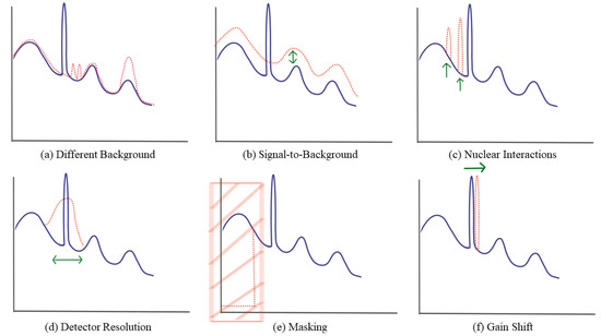
Figure 1.
These augmentations are presented as valid transformations for gamma spectra. They are inspired by radiation detection physics and designed to preserve label invariance (granted that the transformation is not severe). The transformation (red-dotted) upon the original spectrum (dark blue-solid) is indicated with arrows (green).
Nuclear materials of interest to national security are radioactive, meaning they could potentially be measured by a radiation detector. Rapidly identifying these materials (e.g., with machine learning) when they are being transported has a variety of valuable applications, from enabling safety and security for nuclear operators to ensuring monitoring and safeguards for nuclear nonproliferation. Previous work [11] highlighted how SSML could be used to determine—given a measured spectrum—whether a transfer event occurred. Here, given a material transfer spectrum, the classification task is to distinguish what type of material was transferred.
Each augmentation relies on manipulating combinations of decomposed components of the spectrum. Assume that an individual spectrum (binned as a function of energy) can be decomposed into three constituent parts:
where a spectrum () consists of Gaussian-shaped signals () specifically associated with various radioactive sources present during measurement, a slowly varying and characteristic background distribution (), and Poissonian noise (). The spectra in this analysis consist of vectors with 1000 components corresponding to the 1000 energy bins (3 keV each) collected during measurements. Each augmentation manipulates either one or more of a spectrum’s underlying components or an individual feature in that component.
It is necessary for some augmentations to first estimate the background distribution () before transforming the spectrum. This can be difficult to manually extract—even for a subject-matter expert—because background radiation is highly dependent on environmental factors that are unique to every measurement. For example, in a given region of interest () where one signature is present, a common procedure is to fit a Gaussian peak with a linear trend
where the additional fit parameters are the peak’s amplitude (A), the peak’s standard deviation (, related to the peak’s width), the peak’s centroid (), the background’s linear slope (m), and the background’s zero-point (c). This assumes a region of interest sufficiently small enough to capture the peak and its shoulders, where the present background is approximately linear. Equation (2) omits the noise associated with counting statistics for detection setups () because modeling this noise could result in overfitting if successful. This fit procedure is used below when estimating signal peak parameters for manipulation.
Instead of measuring a region of interest’s fit parameters directly, an entire spectrum could be decomposed using an algorithm for Baseline Estimation and Denoising using Sparsity (BEADS) [19]. BEADS was originally developed for chromatograph spectra and decomposes the spectrum using low- and high-pass operators with tunable hyperparameters. A simulated gamma spectrum from a sodium iodide detector was generated with known components of signal, baseline, and noise. The hyperparameters were then tuned to match the BEADS decomposed portions to the known distributions. Refer to Table 1 for the BEADS hyperparameters used in this work when augmenting spectra (Hyperparameter optimization and the values presented in Table 1 were provided by an experienced BEADS user.) Augmentations are then applied to one or a combination of the spectrum components: signals (), background (), or noise ().

Table 1.
Optimized BEADS hyperparameters.
2.2. MINOS Data and Detection Task
For this analysis, gamma radiation spectra collected at the Multi-Informatics for Nuclear Operating Scenarios (MINOS) testbed are used. The MINOS testbed at Oak Ridge National Laboratory (ORNL) collects multimodal data streams relevant to nuclear nonproliferation. This is accomplished using a network of mature sensor technologies distributed around two points of interest at ORNL: the Radiochemical Engineering Development Center (REDC) and High Flux Isotope Reactor (HFIR). The reactor facility (HFIR) is used for scientific experiments (e.g., neutron scattering) and isotope production. Materials generated at HFIR are loaded into shielded casks and are transferred by a variety of methods (e.g., flatbed truck) to REDC. Once at REDC, materials are unloaded, stored, and processed in hot cells.
Material transportation can occur along several routes between HFIR and REDC. Nodes at the MINOS testbed are distributed beside the road along the possible routes. Radiation data are collected using NaI detectors capable of measuring gamma radiation emitted from nearby sources. Assume that all measured spectra have been measured for a 1-min integration time and undergone an energy calibration binned in 1000 channels of 3 keV per bin. A material transfer could occur on the order of tens of seconds or longer. A 1-min integration time ensures that the spectrum has enough statistics for conducting augmentations without being so long as to dominate transfer spectra with background radiation.
A breakdown of all data, unlabeled data, and labeled data can be seen in Figure 2. At a 1-min integration time—with no temporal overlap in integration—there are approximately 9.5 million uncharacterized spectra collected over six nodes and 3 years at the testbed. Since most of the spectra measured over time will be of background, down-sampling will provide a training set more reflective of nuclear material transfers. A spectrum with a weakly anomalous, elevated count rate may be a transfer event or some other type of anomalous environmental radioactive event. Whereas there may be too many weakly anomalous spectra to arbitrate manually, SSML methods can further isolate events of interest, e.g., transfers [11].
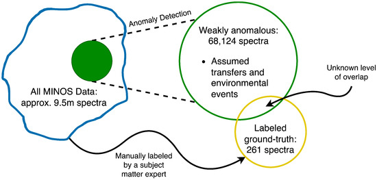
Figure 2.
A breakdown of all MINOS data used in contrastive machine learning. A weakly anomalous subset of the entire dataset (blue) is generated using hypothesis testing anomaly detection with (yellow). The unlabeled, weakly anomalous spectra will be used for contrastive self-supervision. A smaller subset (green) with an unknown amount of overlap with the unlabeled subset was manually labeled using ground truth as a reference by a subject-matter expert. The limited, manually labeled spectra will be used for training the classifier with supervised learning.
A training subset is collected using the hypothesis testing anomaly detection algorithm detailed in previous work [11]. Briefly, assuming total counts are , an anomalous (e.g., transfer) spectrum will have sufficiently different counts to be sampled from a different distribution than consecutive measurements. Radiation counts measured by a gamma detector are governed by a Poisson distribution because gamma radiation emitted from radioactive isotopes are independent events, with a specific probability of decay governed by the half-life of any given decay mechanism. With this discrete likelihood of decay occurring, the measurement is collected at an average interval. The test is then to accept or reject the hypothesis that two consecutive measurements are sampled from the same underlying distribution
using a binomial test
Here, a larger p-value captures more anomalous spectra by applying a looser threshold to changes in gross count rate over time. A p-value of yields 68,124 weakly anomalous spectra. This subset will include some unknown number of transfers, background, and other anomalous event spectra. An even larger p-value could be used, but as p increases, more and more of the entire dataset is captured as anomalous. For example, captures 252,854 spectra, but the increase from only includes spectra that are less anomalous, and therefore, less likely, but not impossible, to be from material transfers. Initial contrastive models that were trained and tested indicated no added benefit to classification accuracy by using over . Likewise, a smaller p-value would capture fewer anomalies, and therefore, have less unlabeled data to contrastively train from. Therefore, produces a large enough training dataset for contrastive learning while limiting the number of included background radiation spectra.
Seven types of transfers occur in the MINOS dataset that can roughly be subdivided into two mutually exclusive classes (see Table 2 [20]). To simulate nuclear nonproliferation scenarios, there are byproducts of the nuclear fuel cycle that may be radioactive or have alternative applications but are not necessarily materials of interest. Contrast these with nuclear material that might be tracked or monitored for proliferation resistance. To demonstrate the utility of contrastive machine learning, the model attempts to distinguish between these two classes. Certainly, many other nonproliferation detection tasks could be designed from this dataset (e.g., multiclass classification for identifying each type of material transfer).
Table 2.
Shielded radiological material transfers present in MINOS data.
A smaller subset of labeled data was prepared for training a supervised classifier. Labeled data were independently prepared and shared by a subject-matter expert, and cross-referenced with ground truth transfer records. In total, 261 spectra spanning the seven transfer subcategories were labeled. Timestamps are not available for these spectra, and the degree of overlap with the unlabeled subset is unknown. Crucially, some spectra may not qualitatively exhibit characteristic features (e.g., photopeaks) associated with their labeled transfer type. This can occur when ground truth data specifies a transfer, but various factors (e.g., background) obfuscate features. A contrastive learning framework and classifier may be able to classify these spectra if it is sensitive enough to transfer type, or these spectra may result in misclassifications or out-of-distribution behavior, resulting in limited classification performance.
2.3. Semi-Supervised Machine Learning
Consider the following dataset of observations (for this analysis, radiation spectra):
consisting of two finite subsets: labeled data and unlabeled data . For a given observable (), its assigned label describes some environmental phenomenon captured by its measurement among a finite set of classes: . The goal of machine learning, therefore, is to construct a model that approximates the relationship between x and y such that labels could be estimated for an unseen measurement:
An optimal model can be found using empirical risk minimization:
Using some form of optimization, a finite number of models can be tested. For supervised models, M is presumably a sufficiently large set such that only labeled data are needed for training (and thus only the supervised loss term is used). In many domains, , making it necessary to incorporate unlabeled data in training. Assuming some necessary [21] relationship between labels and the unlabeled data distribution (e.g., the cluster assumption, manifold assumption, etc. [22]), SSML can successfully learn decision boundaries and outperform supervised learning when labeled data are scarce and classes are sufficiently distinguishable [23].
2.4. Contrastive Machine Learning
Contrastive learning, or self-supervision more broadly, is a set of SSML methods that considers the similarity between data instances. Like other graph-based methods (e.g., Label Propagation [24]), contrastive machine learning uses a notion of distances for making label predictions.
Consider the framework in Figure 3, based on SimCLR [2]. Each unlabeled (or labeled) spectrum, s, in a batch, is augmented twice using two random transformations, with replacement, from the set of transformations (i.e., ). The two transformations randomly generate two augmented spectra, . The representation model, , takes each augmented spectrum as input and outputs a higher dimensional representation.
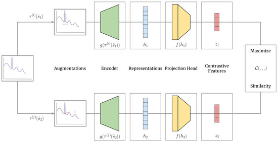
Figure 3.
A contrastive learning framework defined for use with MINOS radiation data. Spectra, s, are perturbed using a transformation, , into augmented spectra, . Augmented spectra serve as input to a representation model, , which provides representations to a projection head, , upon which contrastive learning is ultimately conducted.
These representations become the input of a projection head, , which reduces the dimensionality (thereby distilling significant features or patterns in representations) to an output that is directly used in computing and optimizing a contrastive loss. The reduced dimensionality of projected representations mitigates the curse of dimensionality associated with Euclidean and other distance metrics like cosine similarity. However, this implies that no two representations will appear similar when dimensionality is large.
The projection head also helps to manage noise from data augmentations and encourages pairwise feature independence in resulting representations [25]. An augmentation applied too severely might overwrite labeling information in a spectrum, therefore, breaking label invariance. In this case, it would be inappropriate (or at least suboptimal) to encourage representation similarity. Distilling a representation to a projection dimension dilutes the effect of this scenario by potentially acting as another barrier to overfitting. Finally, pairwise feature independence is valuable for preventing the collapse of output representations to a trivial solution [26].
Once the encoder has been trained, the projection head can be discarded, and a classification model can be used to predict labels (here, byproduct or tracked nuclear material) given a spectral representation. Discarding the projection head for classification tasks has been shown to be beneficial for transfer learning by avoiding the model overfitting from the training [25]. That is, the upstream task (contrastive learning of fundamental patterns in radiation spectra) differs from the downstream task (classifying nuclear material transfers) and pruning helps align the representation model to the downstream task.
Each , created by transforming s, should both have the same label because they contain the same intrinsic labeling information, assuming the transformation is label invariant. The optimization task of contrastive learning is then to ensure that representations are similar for positive pairs. These pairs could be the original spectrum, s, and its transformed value, , or two augmented instances, , from the same source instance. Negative pairs from dissimilar sources should be maximally dissimilar. Therefore, the model contrasts between similar, augmented views of samples—which implies information about an instance’s class—and dissimilar samples in a batch. Note, that the true or observed label is not necessary for contrastive learning (although labeled data could theoretically be used to regularize representations with known labels).
2.5. Alternative Contrastive Methods
Several contrastive and self-supervised models have already been proposed, mostly used on visual modalities. SimCLR [2] does not directly use the original sample image (here, a spectrum) but rather trains a model using only the augmented pairs generated from the image. Alternatively, a bag of visual words representation [27] could be constructed, comparing the original image to an augmented counterpart. The BARLOW TWINS method [4] tunes the representation model by optimizing the cross-correlation in output for augmented samples. One student–teacher method [5] trains a smaller distillation model to effectively generalize. Others apply a stop-gradient [6] so that optimization only occurs along one representation of the input sample. One implementation [7] includes spectral clustering to avoid a requirement for conditional independence and more closely consider class similarity.
Empirical results [10] suggest that self-supervised learning frameworks like contrastive learning can be robust to the class imbalance in select data streams. This is likely because the representations learned are strong enough to discriminate between different types of class distributions. Even though the experiments described above conduct binary classification as an ultimate downstream target task, these models would be beneficial for multinomial classification. Special nuclear material transfers tend to be rare in the MINOS data and potentially nonexistent for certain real-world monitoring applications. If so, a model needs to be tuned and prepared for severe class imbalance to the point of anomaly detection.
Contrastive learning, and self-supervised machine learning broadly, do not intrinsically require labeled data to optimize a model. Contrastive loss functions typically maximize agreement between positive pairs, where positive pairs are defined either as two augmentations of the same data instance or one augmented instance compared with the original. Optimization in this way can be successful if the augmentations—given a known set of transformations—are not severe enough to obscure labeling information present in the unaltered observation. If labeled data are available, fine-tuning can be used to “check answers” in model training or more importantly define the number of classes possible in the dataset. Semi-supervision has an advantage over supervised learning because it can handle unlabeled data and extrapolate labels via known classes.
How else could labeled data be used in self-supervised learning? Typical SSML models are rooted in supervised methods with consistency enforcing functions added to the loss term. Self-supervision is almost the opposite, reminiscent of unsupervised methods. One such example trains a larger model contrastively and then prunes the model, or makes it smaller, by a process of supervised fine-tuning [28]. Another example, supervised contrastive learning [29], uses labeled data as anchor points for the broader data distribution, further defining positive pairs and adding generalization weight to contrastive learning. Finally, another example uses the similarity between samples to gradually group classes: weakly supervised contrastive learning [30].
2.6. Normalized Cross-Entropy Loss
The loss function used in SimCLR is a generalization of N-Pairs Loss, dubbed the normalized temperature-scaled cross-entropy loss (or NT-XENT). Elsewhere, this loss function is titled INFO NCE [31,32]. Given a set of data augmentations, samples are fed through a base encoder, which produces a representation. There are no constraints on this encoder in SimCLR, varying strategies include producing higher-dimensional representations, an encoder/decoder pair, convolution followed by average pooling, etc., SimCLR observed that attaching a projecting head consisting of a single hidden layer with a ReLU activation function is beneficial for applying and optimizing contrastive loss.
The projection head reduces the dimensionality of the representations to what is fed to the contrastive loss function. The training algorithm for SimCLR is as follows: For a given batch of batch size N, produce two augmentations for each, resulting in (augmented) samples. Each pair of augmented samples produces a pair of encoded representations, , derived from the same sample (), which are considered a positive pair; the other samples are assumed as negatives.
For two nonzero vectors, where is the angle between the two vectors, their cosine similarity is
which varies in the range . This serves as a distance metric, or difference measure, between the two vectors (i.e., two input samples). NT-XENT loss is then the cross-entropy of cosine similarities for the projected representations of positive pairs , normalized over all pairs
The temperature coefficient, , acts as a fixed hyperparameter scaling the magnitude of similarities. Note, that the denominator sums over the first input, , paired with all other samples but itself. If, for example, , then their cosine similarity will be 1, and (assuming ) the first term of Equation (9) will be . If , then their cosine similarity will be 0, and the first term of Equation (9) will be . In practice, many negative pairs will not be exactly orthogonal to the anchor point (i.e., the first input), and therefore, the cosine similarity in the second term will be nonzero, meaning the minimum might not be precisely even if the positive pair is identical. However, the additional loss for negative pairs encourages them to be maximally dissimilar, i.e., assuming , an optimal solution would have for positive pairs and for negative pairs. Therefore, minimizing the loss function achieves two goals: maximizing similarity between positive pairs and minimizing similarity between negative pairs. Finally, the loss is averaged for all positive pairs in each direction:
Even though cosine similarity is a symmetric distance metric (i.e., , because the denominator of Equation (9) will change depending on the anchor point of , resulting in both terms being computed in Equation (10).
In summary, the loss function optimizes the encoder to maximize similarity in output representations for augmented spectra derived from the same original spectrum and maximize dissimilarity for all other representations in a batch. Note, that this process does not strictly require knowledge of the true labels for augmented spectra and is, therefore, nominally a self-supervised method. If the augmentations used are label-invariant, then a positive pair of augmented samples are assumed to have the same underlying label as that of their parent, regardless of what that label may be. After successfully training a contrastive machine learning model, the representations of spectra sharing the same label (whatever that label is) should be clustered in the encoder’s state space (i.e., have minimal notional distance).
3. Method
3.1. Model Architecture
A pictorial representation of the contrastive learning framework can be seen in Figure 4. An encoder produces high-dimensional representations from spectra. These representations still reside in a one-dimensional embedding space but of length up to four times the original length of the spectra. The projection head produces projections from the representations with reduced dimensionality, broadly less than that of the original spectrum length (see Figure 4a). The representation model is optimized using Adam [33].
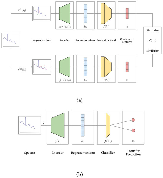
Figure 4.
Illustration of the framework during contrastive machine learning (from Figure 3) with a (a) projection head and when training and testing with a supervised (b) classifier. Spectra passed through an encoder generate higher dimensional representations that, when projected, can be used to compute and minimize a contrastive loss. The projection head is replaced by a classifier that takes high-dimensional representations and produces class probability.
After contrastive training, when the projection head is discarded, a classifier is trained directly on the representations (see Figure 4b). The classifier used here is a one-layer linear model that takes the representation features and produces two class probabilities: one for byproducts and one for nuclear material transfers. This simple classifier in itself may not be complex enough to capture the relationships between representations and labels, but it allows observed increases in accuracy to be the result of contrastively learned information by the encoder. The largest class probability is the designated label for any spectrum in the training or testing dataset. The classifier is trained using the Limited-memory Broyden–Fletcher–Goldfarb–Shanno (L-BFGS) algorithm in PYTORCH via supervision by a labeled subset with cross-entropy loss penalizing disagreement between estimated and expected labels.
3.2. Hyperparameter Optimization
The Tree-structured Parzen Estimator approach [34,35] was used to choose optimized hyperparameter values over several successive trials. The model is taken to be sufficiently converged after 100 epochs as loss minimization has considerably reduced. Sharp increases in loss are the result of the optimizer attempting to escape local loss minima. The optimized representation model was a Multilayer Perceptron (MLP) with three hidden layers of lengths 4096, 2048, and 4096, and an output representation length of 2048. The optimized projection head had one hidden layer matching the length of the encoder’s output and a projection length of 527.
Once optimal parameters for the encoder and projection head are found, several trials of optimization are conducted to optimize the learning rate and regularization weight for the linear classifier. The two hyperparameters optimized for the classifier belong to the Adam optimization algorithm from PYTORCH with L2 regularization. The actual learning rate for contrastive learning is determined by scaling the base learning rate, dependent on the batch size, according to
This scaling helps stabilize training when batch size is large [25]. Here, hyperparameters are chosen to maximize the average balanced accuracy score from fivefold cross-validation (trained on 20%, tested on 80% of labeled data).
The sorted scores for all linear classifiers tested are shown in Figure 5. Some classifiers have poor accuracy performance, corresponding to models trained with extreme hyperparameter values. Most classifiers maintain a relatively consistent average balanced accuracy score owing to stable convergence for cross-validated classifiers independent of hyperparameter value. Some models achieved a much higher average balanced accuracy score. Results for the model with the highest balanced accuracy score from the trial with the highest average cross-validation performance will be shown below.
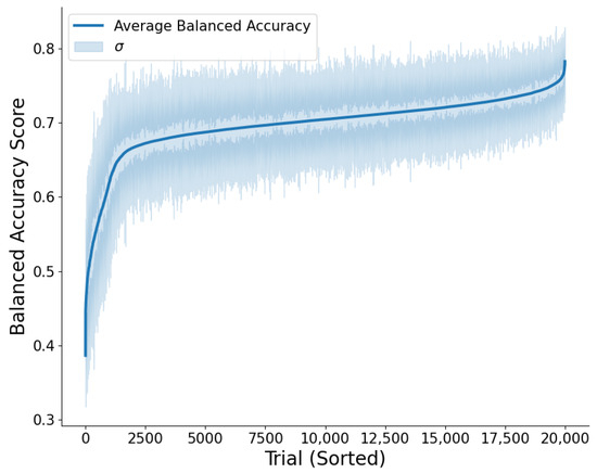
Figure 5.
The classifier test results for all 20,000 trials conducted during hyperparameter optimization for the classifier. Since each trial conducted 5-fold cross-validation, the average balanced accuracy (blue) is reported, and the trials are sorted according to this magnitude (i.e., this is not the serial order in which trials were executed). One standard deviation—as calculated by the five balanced accuracy scores reported for each trial—is plotted (blue shaded region). Note, that the standard deviation is noisy, even for trials with comparable average balanced accuracies.
4. Results
The best trial achieved an average balanced accuracy score of 78.22%. The balanced accuracy score for every cross-validation fold for this best iteration is reported in Table 3. As a benchmark, the best model of the five trained and tested in cross-validation for this best trial will be used. For the best model from the best trial, which achieved a balanced accuracy score of 80.30%, the confusion matrix of test spectra is plotted in Figure 6.
Table 3.
Cross-validation balanced accuracy scores for the highest average achieved.
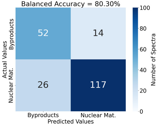
Figure 6.
A confusion matrix for test spectra passed to the best model from the best trial trained after all sequences of hyperparameter optimization (encoder, projector, and classifier). This model’s balanced accuracy score is 80.30%, tested on 80% of the labeled dataset. Compared to the previous model tested, this model is more successful at detecting nuclear material transfers and less successful at detecting byproducts.
To analyze systematic misclassifications further, the test results categorized for each subclass are presented in Figure 7c,d for byproducts and tracked nuclear material transfers, respectively. The model appears to have better detection accuracy for 252Cf and irradiated Cm than it does for Np transfers (unirradiated or irradiated). The model appears to have the best success at detecting 225Ac among the byproduct subclasses. Both results suggest some form of pattern recognition that is advantageous for specific types of transfers.
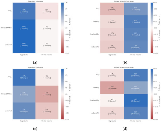
Figure 7.
Training and testing classification accuracy summaries for each subclass in the byproduct class (i.e., all instances have a true binary label of byproduct) and in the nuclear material class (i.e., all instances have a true binary label of nuclear material). In each cell, the percent (and gross number) of test spectra labeled a given binary class are listed. Increasingly successful classification rates are shaded blue, increasing misclassification rates are shaded red. (a) Byproduct transfer training samples. (b) Tracked material transfer training samples. (c) Byproduct transfer test samples. (d) Tracked material transfer test samples.
Note, that the linear classifier did not achieve 100% training accuracy, as shown in Figure 7a,b for byproducts and nuclear material transfers, respectively. Instead, the model appears to achieve the best training detection accuracy for activated metals and spent fuel transfers despite (or perhaps because of) only having a handful of training spectra for those transfer types. The relation between training misclassifications, testing misclassifications, and a definitive decision boundary is difficult to assess. The lower performance on training data may be the cause of success in testing data, or it could be detrimental. Perhaps another version of this model—trained on the same data but at a different initialization—may perform better or worse. From a nonproliferation perspective, failing to detect a tracked nuclear material would be a higher consequence than failing to detect a byproduct shipment. Evaluating the value of a given detection model depends on an asymmetric penalty function, where false negatives would be weighted higher than false positives.
5. Discussion
The contrastive self-supervision learns and accentuates spectral features associated with radiation sources in a task-agnostic manner using label-invariant spectral augmentations. The trained encoder should have a richer state space by virtue of embedded information learned from unlabeled data. The linear classifier used in the contrastive framework above has limited complexity and could be replaced by any number of other classifiers. Popular methods are available in the SCIKIT-LEARN package (version 1.2.2), for example, logistic regression, MLP, Support Vector Machine (SVM), and Label Propagation. Each method (except Label Propagation) is strictly supervised, meaning they can only train on labeled data. These methods may be successful on large volumes of well-curated data, but their performance will be hindered when labeled data are limited, noisy (i.e., possibly mislabeled), and labeling information is possibly obscured (i.e., photopeaks occluded by background radiation).
For example, consider a scenario where limited labeled data are available, and each of the methods mentioned above is trained and tested using the spectra directly as input features. Using the 261 labeled spectra from MINOS (see Figure 2), a training subset of 52 spectra (20%) and a testing subset consisting of 209 spectra (80%) are created. Typical practice for cross-validation is to use a leave-one-out strategy (i.e., use one partition for testing, the rest for training). The opposite was used here to accentuate the effects of conducting supervised learning with limited labeled data (i.e., use one partition for training, the rest for testing). Fivefold cross-validation is used to average the resulting accuracy and avoid training bias associated with a specific cut of the labeled dataset. These supervised classifiers are only able to utilize the limited labeled dataset of 52 spectra.
Consider also a scenario in which the same classifiers–trained on the same limited labeled dataset–use representations generated from the contrastively trained encoder above as input features instead of the spectra directly. Using the encoder allows these supervised classifiers to leverage embedded information learned from unlabeled data.
Compare the two scenarios in Table 4. Fivefold cross-validation average balanced accuracy scores are reported for each supervised classifier using spectra as inputs and representations as inputs. For completeness, the linear model from Section 4 is also reported. Using an encoder contrastively trained with unlabeled data results in a higher average test accuracy than using the labeled spectra alone, regardless of the type of classifier used. In this way, contrastive learning alleviates the cost of labeling spectra by leveraging unlabeled data to improve classification accuracy.
Table 4.
Cross-validation using five folds on various SCIKIT-LEARN algorithms. Highest accuracy per model are bolded, best overall is italicized. The results from Table 3 are also summarized.
Given the consistent improvement in estimates of the classification targets when using the spectral representations as inputs to the interpretative models rather than the raw spectra, independent of the model type, the utility of constructing the embeddings is clear. To aid in understanding these results, briefly consider the situation from a statistical estimation perspective.
The raw spectra and source type are the observed random variables and random variables to be estimated (targets), respectively. Although the observed random variables are informative and predictive of the associated target variables, most of the components are uninteresting with respect to the targets (i.e., they are informationally sparse, hence they may be suitable for latent space projection methods). In traditional spectral analysis, the interesting random variable components, the spectral peaks, are located, analyzed, and compared to nuclear data to identify and quantify the constituent gamma-emitting radionuclides. Given this derived information, which comprises latent random variables, classification in terms of the type of material transfer is relatively straightforward. The primary shortcoming of material transfer classification is the effort and time incurred in the manual analysis required to derive the latent variables through a physics-designed signal processing workflow.
Intuition suggests high-capacity data analytic models such as large neural networks are capable of implicitly discovering these latent variables to yield accurate classification estimates, but developing and carefully tuning such models requires large numbers of labeled examples (i.e., annotated spectra), which precludes their use in this application. As shown in Section 4, contrastive learning with physics-informed label-invariant data augments is able to develop an embedding or spectral representation that is approximately equivalent to a map to the latent random variables discussed above based on their capability to allow a downstream supervised classifier to accurately estimate transfer types with small numbers of labeled examples for training. In both the manual analysis designed by physics and physics-informed data-driven approach using contrastive learning, the physics of gamma-ray spectra are used to find the latent random variables to improve and enable high-quality classification; however, this data-driven approach is more amenable to automation and high throughput at the expense of explicit interpretability and transparency. In the future, investigating this interpretation further with model explainability methods such as Shapley factors to better understand the performance and characteristics of the spectral representations derived by contrastive learning workflow may be warranted.
6. Conclusions
Carefully characterizing the necessary volumes of labeled data for use in machine learning applications can be challenging in nuclear nonproliferation even when synthetic data generation is feasible. Gamma spectra, despite being a potentially impactful observation modality, often require manual analysis to detect the presence of nuclear sources. Manual analysis can be time-consuming, highly variable, and dependent on subject-matter expertise. These problems might become intolerably resource-intensive when the number of spectra needed to adjudicate alarms or anomalies increases, either because of an increasingly large sensor network or longer collection periods. Artificial intelligence has the potential to alleviate the cost of the manual analysis of spectra, but the current regime of manual analysis is too costly to generate the necessary training data to implement artificial intelligence systems.
This work applied contrastive semi-supervised machine learning to develop a methodology for making the analysis of radiation spectra for nuclear security more efficient. To demonstrate this capability, semi-supervised machine learning is used on gamma spectra from the MINOS testbed at ORNL (collected with limited ground truth) to detect and characterize the transfer of shielded radiological material. Label-invariant gamma radiation augmentations were applied to weakly anomalous spectra and an encoder was contrastively trained to maximize similarity in pairs of output representations. A supervised linear classifier was trained on 52 labeled samples to take encoded spectra and predict a binary classification label: byproduct or tracked nuclear material. The hyperparameter-optimized model showed promising balanced accuracy (80.30%). More complex classifiers performed better on representations than directly on spectra, further demonstrating the efficacy of contrastive machine learning on spectra.
Author Contributions
Conceptualization, J.R.S., P.P.H.W. and K.J.D.; software, J.R.S. and P.P.H.W.; formal analysis, J.R.S.; investigation, J.R.S., P.P.H.W. and K.J.D.; writing—original draft preparation, J.R.S.; writing—review and editing, J.R.S., P.P.H.W. and K.J.D.; visualization, J.R.S.; supervision, P.P.H.W. and K.J.D.; project administration, P.P.H.W. and K.J.D. All authors have read and agreed to the published version of the manuscript.
Funding
This work is supported by the Department of Energy/National Nuclear Security Administration under award number DE-NA0003921.
Data Availability Statement
Restrictions apply to the availability of these data. Data were generated at Oak Ridge National Laboratory and are available with the permission of the U.S. Department of Energy, National Nuclear Security Administration, Office of Defense Nuclear Nonproliferation Research and Development.
Acknowledgments
The authors are thankful for the support of the MINOS collaboration at Oak Ridge National Laboratory for collecting, organizing, and sharing the data used in this project, particularly Daniel Archer, James Ghawaly, Andrew Nicholson, and Michael Willis. The authors thank Jason Hite and Birdy Phathanapirom for their help in editing and reviewing this paper. Thanks also to Jason Hite for providing the hyperparameter values used for BEADS. The authors would also like to thank Robert Nowak and Danica Fliss at the University of Wisconsin–Madison for their collaboration and guidance on machine learning and hypothesis testing.
Conflicts of Interest
The authors declare no conflicts of interest.
References
- IAEA Safeguards Glossary; Number 3 (Rev. 1) in International Nuclear Verification Series; International Atomic Energy Agency: Vienna, Austria, 2022.
- Chen, T.; Kornblith, S.; Norouzi, M.; Hinton, G. A Simple Framework for Contrastive Learning of Visual Representations. arXiv 2020, arXiv:2002.05709. [Google Scholar]
- Phathanapirom, B.; Hite, J.; Dayman, K.; Chichester, D.; Johnson, J. Improving an Acoustic Vehicle Detector Using an Iterative Self-Supervision Procedure. Data 2023, 8, 64. [Google Scholar] [CrossRef]
- Zbontar, J.; Jing, L.; Misra, I.; LeCun, Y.; Deny, S. Barlow Twins: Self-Supervised Learning via Redundancy Reduction. In Proceedings of the 38th International Conference on Machine Learning, PMLR, Virtual, 18–24 July 2021; Volume 139, pp. 12310–12320. [Google Scholar]
- Fang, Z.; Wang, J.; Wang, L.; Zhang, L.; Yang, Y.; Liu, Z. SEED: Self-supervised Distillation for Visual Representation. In Proceedings of the International Conference on Learning Representations, Virtual Event, Austria, 3–7 May 2021. [Google Scholar]
- Grill, J.B.; Strub, F.; Altché, F.; Tallec, C.; Richemond, P.; Buchatskaya, E.; Doersch, C.; Avila Pires, B.; Guo, Z.; Gheshlaghi Azar, M.; et al. Bootstrap Your Own Latent—A New Approach to Self-Supervised Learning. In Proceedings of the Advances in Neural Information Processing Systems, Online, 6–12 December 2020; Curran Associates Inc.: Red Hook, NY, USA, 2020; Volume 33, pp. 21271–21284. [Google Scholar]
- HaoChen, J.Z.; Wei, C.; Gaidon, A.; Ma, T. Provable Guarantees for Self-Supervised Deep Learning with Spectral Contrastive Loss. In Proceedings of the 35th Conference on Neural Information Processing Systems (NeurIPS 2021), Online, 6–14 December 2021. [Google Scholar]
- Stomps, J.; Wilson, P.; Dayman, K.; Willis, M.; Ghawaly, J.; Archer, D. Data Augmentations for Nuclear Feature Extraction in Semi-Supervised Contrastive Machine Learning; Institute of Nuclear Materials Management: Deerfield, IL, USA, 2022. [Google Scholar]
- Jaiswal, A.; Babu, A.R.; Zadeh, M.Z.; Banerjee, D.; Makedon, F. A Survey on Contrastive Self-Supervised Learning. Technologies 2021, 9, 2. [Google Scholar] [CrossRef]
- Liu, H.; HaoChen, J.Z.; Gaidon, A.; Ma, T. Self-supervised Learning is More Robust to Dataset Imbalance. In Proceedings of the NeurIPS 2021 Workshop on Distribution Shifts: Connecting Methods and Applications, Virtual, 13 December 2021. [Google Scholar]
- Stomps, J.R.; Wilson, P.P.H.; Dayman, K.J.; Willis, M.J.; Ghawaly, J.M.; Archer, D.E. SNM Radiation Signature Classification Using Different Semi-Supervised Machine Learning Models. J. Nuclear Eng. 2023, 4, 448–466. [Google Scholar] [CrossRef]
- Ma, J.; Jiang, J. Semisupervised Classification for Fault Diagnosis in Nuclear Power Plants. Nuclear Eng. Technol. 2015, 47, 176–186. [Google Scholar] [CrossRef][Green Version]
- Sun, L.; Zhao, C.; Yan, Z.; Liu, P.; Duckett, T.; Stolkin, R. A Novel Weakly-Supervised Approach for RGB-D-Based Nuclear Waste Object Detection. IEEE Sens. J. 2019, 19, 3487–3500. [Google Scholar] [CrossRef]
- Moshkbar-Bakhshayesh, K.; Ghofrani, M.B. Combining Supervised and Semi-Supervised Learning in the Design of a New Identifier for NPPs Transients. IEEE Trans. Nuclear Sci. 2016, 63, 1882–1888. [Google Scholar] [CrossRef]
- Moshkbar-Bakhshayesh, K.; Mohtashami, S. Classification of NPPs Transients Using Change of Representation Technique: A Hybrid of Unsupervised MSOM and Supervised SVM. Prog. Nuclear Energy 2019, 117, 103100. [Google Scholar] [CrossRef]
- Stomps, J.R. Gamma Spectroscopy Data Augmentation for Self-Supervised Machine Learning Applications to Nuclear Nonproliferation on Measured Data with Limited Ground-Truth; The University of Wisconsin-Madison: Madison, WI, USA, 2023. [Google Scholar]
- Krane, K.S. Introductory Nuclear Physics; Wiley: New York, NY, USA, 1988. [Google Scholar]
- Knoll, G. Radiation Detection and Measurement, 4th ed.; John Wiley: Hoboken, NJ, USA, 2010. [Google Scholar]
- Ning, X.; Selesnick, I.W.; Duval, L. Chromatogram Baseline Estimation and Denoising Using Sparsity (BEADS). Chemom. Intell. Lab. Syst. 2014, 139, 156–167. [Google Scholar] [CrossRef]
- Dayman, K.; Hite, J.; Hunley, R.; Rao, N.S.V.; Geulich, C.; Willis, M.; Ghawaly, J.; Archer, D.; Johnson, J. Tracking Material Transfers at a Nuclear Facility with Physics-Informed Machine Learning and Data Fusion; Institute of Nuclear Materials Management: Deerfield, IL, USA, 2021. [Google Scholar]
- Lu, T. Fundamental Limitations of Semi-Supervised Learning. Master’s Thesis, University of Waterloo, Waterloo, ON, Canada, 2009. [Google Scholar]
- Chapelle, O.; Schölkopf, B.; Zien, A. Semi-Supervised Learning; MIT Press: Cambridge, MA, USA, 2006. [Google Scholar]
- Singh, A.; Nowak, R.; Zhu, J. Unlabeled Data: Now it Helps, Now it Doesn’t. In Proceedings of the Advances in Neural Information Processing Systems, Vancouver, Canada, 8–10 December 2008; Curran Associates Inc.: Red Hook, NY, USA, 2008; Volume 21. [Google Scholar]
- Zhu, X.; Ghahramani, Z. Learning from Labeled and Unlabeled Data with Label Propagation; Carnegie Mellon University Technical Report CMU-CALD-02-107; Carnegie Mellon University: Pittsburgh, PA, USA, 2002. [Google Scholar]
- Balestriero, R.; Ibrahim, M.; Sobal, V.; Morcos, A.; Shekhar, S.; Goldstein, T.; Bordes, F.; Bardes, A.; Mialon, G.; Tian, Y.; et al. A Cookbook of Self-Supervised Learning. arXiv 2023, arXiv:cs.LG/2304.12210. [Google Scholar]
- Mialon, G.; Balestriero, R.; LeCun, Y. Variance Covariance Regularization Enforces Pairwise Independence in Self-Supervised Representations. arXiv 2024, arXiv:2209.14905. [Google Scholar]
- Gidaris, S.; Bursuc, A.; Komodakis, N.; Perez, P.; Cord, M. Learning Representations by Predicting Bags of Visual Words. In Proceedings of the IEEE/CVF Conference on Computer Vision and Pattern Recognition (CVPR), Seattle, WA, USA, 14–19 June 2020. [Google Scholar]
- Chen, T.; Kornblith, S.; Swersky, K.; Norouzi, M.; Hinton, G.E. Big Self-Supervised Models are Strong Semi-Supervised Learners. In Proceedings of the Advances in Neural Information Processing Systems, Online, 6–12 December 2020; Larochelle, H., Ranzato, M., Hadsell, R., Balcan, M., Lin, H., Eds.; Curran Associates Inc.: Red Hook, NY, USA, 2020; Volume 33, pp. 22243–22255. [Google Scholar]
- Khosla, P.; Teterwak, P.; Wang, C.; Sarna, A.; Tian, Y.; Isola, P.; Maschinot, A.; Liu, C.; Krishnan, D. Supervised Contrastive Learning. In Proceedings of the Advances in Neural Information Processing Systems, Online, 6–12 December 2020; Curran Associates Inc.: Red Hook, NY, USA, 2020; Volume 33, pp. 18661–18673. [Google Scholar]
- Zheng, M.; Wang, F.; You, S.; Qian, C.; Zhang, C.; Wang, X.; Xu, C. Weakly Supervised Contrastive Learning. In Proceedings of the IEEE/CVF International Conference on Computer Vision (ICCV), Montreal, QC, Canada, 11–17 October 2021; pp. 10042–10051. [Google Scholar]
- van den Oord, A.; Li, Y.; Vinyals, O. Representation Learning with Contrastive Predictive Coding. arXiv 2018, arXiv:1807.03748. [Google Scholar]
- He, K.; Fan, H.; Wu, Y.; Xie, S.; Girshick, R. Momentum Contrast for Unsupervised Visual Representation Learning. In Proceedings of the Proceedings of the IEEE/CVF Conference on Computer Vision and Pattern Recognition (CVPR), Seattle, WA, USA, 14–19 June 2020. [Google Scholar]
- Loshchilov, I.; Hutter, F. Fixing Weight Decay Regularization in Adam. arXiv 2017, arXiv:1711.05101. [Google Scholar]
- Bergstra, J.; Yamins, D.; Cox, D. Making a Science of Model Search: Hyperparameter Optimization in Hundreds of Dimensions for Vision Architectures. In Proceedings of the Machine Learning Research, Atlanta, GA, USA, 17–19 June 2013; Volume 28, pp. 115–123. [Google Scholar]
- Bergstra, J.; Bardenet, R.; Bengio, Y.; Kégl, B. Algorithms for Hyper-Parameter Optimization. In Proceedings of the Advances in Neural Information Processing Systems, Granada, Spain, 12–15 December 2011; Curran Associates Inc.: Red Hook, NY, USA, 2011; Volume 24. [Google Scholar]


Disclaimer/Publisher’s Note: The statements, opinions and data contained in all publications are solely those of the individual author(s) and contributor(s) and not of MDPI and/or the editor(s). MDPI and/or the editor(s) disclaim responsibility for any injury to people or property resulting from any ideas, methods, instructions or products referred to in the content. |
© 2024 by the authors. Licensee MDPI, Basel, Switzerland. This article is an open access article distributed under the terms and conditions of the Creative Commons Attribution (CC BY) license (https://creativecommons.org/licenses/by/4.0/).