Abstract
Deceptive path planning (DPP) aims to find routes that reduce the chances of observers discovering the real goal before its attainment, which is essential for addressing public safety, strategic path planning, and preserving the confidentiality of logistics routes. Currently, no single metric is available to comprehensively evaluate the performance of deceptive paths. This paper introduces two new metrics, termed “Average Deception Degree” (ADD) and “Average Deception Intensity” (ADI) to measure the overall performance of a path. Unlike traditional methods that focus solely on planning paths from the start point to the endpoint, we propose a reverse planning approach in which paths are considered from the endpoint back to the start point. Inverting the path from the endpoint back to the start point yields a feasible DPP solution. Based on this concept, we extend the existing method to propose a new approach, , and introduce two novel methods, Endpoint DPP_Q and LDP DPP_Q, based on the existing DPP_Q method. Experimental results demonstrate that achieves significant improvements over (an overall average improvement of 8.07%). Furthermore, Endpoint DPP_Q and LDP DPP_Q effectively address the issue of local optima encountered by DPP_Q. Specifically, in scenarios where the real and false goals have distinctive distributions, Endpoint DPP_Q and LDP DPP_Q show notable enhancements over DPP_Q (approximately a 2.71% improvement observed in batch experiments on 10 × 10 maps). Finally, tests on larger maps from Moving-AI demonstrate that these improvements become more pronounced as the map size increases. The introduction of ADD, ADI and the three new methods significantly expand the applicability of and DPP_Q in more complex scenarios.
MSC:
68T42
1. Introduction
Deception has long been a focal point in computer science, representing a significant hallmark of intelligence [1]. In fields like multi-agent systems and robotics, path planning serves as a foundational element for achieving collaborative task objectives. Deception becomes pivotal in enabling agents to gain strategic advantages in games and adversarial settings. In adversarial environments, deceptive planning empowers both human and AI agents to obscure their true intentions and manipulate the situational awareness of opponents. Beyond gaming contexts, deception is prevalent in diverse multi-agent applications, including negotiations [2,3] and fugitive pursuit scenarios [4]. In adversarial contexts, deceptive planning allows intelligence operatives to obfuscate their true intentions and confound the awareness of adversaries, thereby finding practical use in domains such as network security [5], robot soccer competitions [6], privacy preservation [7], and other real-world challenges. Deceptive path planning (DPP) has thus emerged as a pivotal task within this broader landscape.
Imagine a scenario in urban surveillance in which SWAT teams have located traces of terrorists on city streets. If SWAT teams reveal their intentions and proceed directly to the hideout of terrorists, they risk alarming them, potentially leading to escape. Therefore, the teams can strategize a decoy route, departing from a designated point and feigning a circuitous advance towards other locations to mislead the adversaries. This strategy aims to deceive terrorists into believing that SWAT teams’ objective is not their actual hiding place. Ultimately, the SWAT teams can reach and apprehend or eliminate terrorists. The purpose of this approach is to deceive the surveillance systems and observers of terrorists, thereby concealing the true objective of the SWAT teams to the fullest extent possible.
Consider a scenario in wildlife conservation in where researchers select suitable areas within a vast protected area to reintroduce endangered species. Poachers are monitoring the movement of these animals for their illegal hunting activities. Directly approaching the habitat of these animals can jeopardize their safety. Conversely, planning a circuitous route would deceive potential poachers, ensuring the safety of the animals while minimizing the risk of detection.
Previous research on DPP problems has raised several issues and opportunities for improvement. Firstly, while Masters et al. proposed three metrics (extent, magnitude, and destiny) for evaluating deceptive paths [8], each has its limitations. Extent and destiny merely assess whether grid points along a path are deceptive or not, a binary evaluation without quantifying deception on a scale from 0 to 1. Although magnitude quantifies deception, it lacks normalization. DPP_Q [9], incorporating the concept of “average deceptiveness”, considers paths under specific time constraints where all paths have equal costs, failing to address how paths with varying time costs should be compared. Therefore, unified metrics for comprehensively evaluating the performance of deceptive paths are lacking.
Secondly, DPP_Q tends to fall into local optima when the number of false goals increases. Our experiments indicate that agents trained using the DPP_Q method exhibit a tendency to initially move towards false targets from the starting point. While this approach may yield substantial rewards initially, the fixed time constraints of DPP_Q prevent agents from balancing deception in the subsequent planning phases. Figure 1a illustrates this phenomenon using a heatmap based on a 49 × 49 grid map from the Moving-AI dataset, devoid of obstacles. The orange square (with a black border) represents the start point, the blue square (with a black border) is the real goal, and the teal squares (with black borders) are two false goals. The heatmap visualizes the posterior probability of the real goal at each grid point, ranging from 0 to 1, influencing the agent to bypass the lighter-colored points for greater deception (reward). When the agent begins exploring from the starting point, it tends to follow the direction indicated by the red arrow initially, which is detrimental to subsequent planning. Conversely, following the green arrow direction may not yield immediate rewards but offers greater potential rewards later. In Figure 1b, starting planning from the real goal allows the agent to avoid biased initial exploration tendencies influenced by the heatmap.
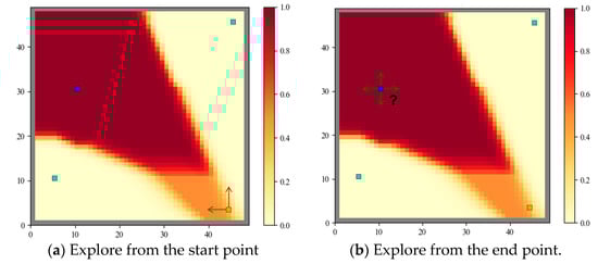
Figure 1.
The heatmap representation of the reward function for the observed correlates with the elements of the DPP problem. Here, the orange square (with a black border) represents the start point, the blue square (with a black border) denote the real goal, and the teal squares (with black borders) signify two false goals.
Thirdly, the initial exploration tendency exhibited by the agent in DPP_Q resembles that of [8]. guides the agent towards false goals initially before proceeding to the real goal, contrasting with methods lacking such tendencies. This distinction typically results in achieving greater deceptive effects compared to methods and explains why paths generated by entail longer costs. Therefore, we propose that the methods could be further optimized based on the tendency of the method. One potential improvement involves adjusting the Last Deceptive Point (LDP), a concept to be detailed later.
This article has three main technical contributions. Firstly, we introduced the concept of Average Deception Degree (ADD), based on which we proposed the Average Deception Intensity (ADI) and analyzed its rationality, applying it to evaluate subsequent methods. Secondly, for methods that do not consider time constraints, we proposed , which can significantly enhance traditional methods. Thirdly, for DPP_Q which considers time constraints, we propose Endpoint DPP_Q and LDP DPP_Q, both resolving issues of suboptimal DPP problems under specific distributions of goals.
The structure of this paper is as follows: In Section 2, we review the relevant literature on probabilistic goal recognition and DPP problems. Section 3 provides foundational definitions of these concepts. Section 4 defines ADD and ADI briefly, introduces methods and subsequently proposes . Subsequently, in Section 4 we introduce DPP_Q, outlining the operational mechanisms of the new methods Endpoint DPP_Q and LDP DPP_Q. In Section 5, based on the ADI, we validate the feasibility of our methods through experiments. Lastly, we conclude with a summary and outlook for this paper.
2. Related Work
2.1. Plan Recognition and Probabilistic Goal Recognition
In the study of agent goal recognition, two key factors are often considered: the competitive dynamics and the level of rationality exhibited by the observed agents. The relationship between the observer and the observed can be categorized into Keyhole scenarios [10], where observed agents are indifferent to the observer’s behavior due to the absence of competitive or cooperative interactions; Adversarial scenarios [11], where observed agents adopt a hostile stance towards the observer’s actions; and Intended scenarios [12], where observed agents cooperate openly with the observer, sometimes assisting in the recognition process. DPP problems primarily focus on adversarial scenarios.
The problem of goal recognition has been explored using various approaches, including graph coverage on planning graphs [13], parsing using grammar methods [14,15,16,17], deduction and probabilistic reasoning on static or dynamic Bayesian networks [18,19], and inverse planning models [20,21]. Bui et al. [22] introduced an online probabilistic plan recognition framework based on Abstract Hidden Markov Models (AHMM). Ramirez and Geffner aligned observed outcomes with predefined plans, computing costs separately for each potential goal [23]. Assuming agent rationality allows for the evaluation of goal types. Masters et al. [24] proposed a traditional cost-difference-based goal recognition model that, estimates goal probabilities based on cost disparities between optimal paths matching current observations and those that ignore specific nodes in the observation sequence.
2.2. Deception and Deceptive Path Planning
Initially, “deceptive information” emerged as a significant focus in deception research. Floridi proposed that “misinformation is structurally well-formed, meaningful false data, whereas deceptive information is intentionally transmitted false information designed to mislead the recipient” [25]. Fetzer [26] categorized five types of deceptive information: intentional misinformation created by information producers to distort and mislead targets, deceptive information formed through selective filtering and sophistry against existing information, deceptive information disseminated by information disseminators attacking information producers based on reasons unrelated to or misleading from the stance represented by the information producer, deceptive information generated based on irrational beliefs, and deceptive information resulting from incompetent commentary. Fallis [27] summarized three characteristics of deceptive information: it is a type of information with the basic attributes of information, it is misleading information, and it is not accidental or unintentional.
Deception also has a long history in computer science, especially holding prominence in artificial intelligence research and game theory. In particular, the article “Deceptive AI” [28] provides a detailed analysis of common types of deception, different characteristics, and typical application scenarios. By referencing examples from various branches of artificial intelligence, this article categorizes deception research into five new categories and describes them based on human-like features: imitating, obfuscating, tricking, calculating, and reframing. Bell et al. proposed a balanced approach to belief manipulation and deception [29], where agents have only a coarse understanding of their opponents’ strategies and little knowledge of details. This method can be viewed as a game theory setting, expressed in terms of social psychology as “fundamental attribution error.” It is often applied to bargaining problems, revealing that deceptive strategies may be more easily executed. Arkin et al. [30] mentioned that deception has always been used as a means to gain military advantage.
Masters et al. [8] formalized Deceptive Path Planning (DPP) problems in path planning domains, demonstrating that qualitative comparisons of posterior probabilities of goals do not necessarily require the entire observation sequence but only the last node. They introduced the concept of the Last Deceptive Point (LDP) and proposed traditional DPP methods based on the A* algorithm and heuristic pruning. These methods prioritize “dissimulation” without precise quantification of each grid’s deceptiveness and do not explicitly model time constraints. Cai et al. [31] researched DPP in dynamic environments using two-dimensional grid maps. Xu et al. [32] applied mixed-integer programming to estimate grid deceptiveness based on magnitude, proposing a method that combines time consumption and quantified deceptiveness. Liu et al. [33] introduced the Ambiguity Model, which integrates optimal Q-values of path planning with deceptiveness to derive ambiguous paths. Lewis [34] addressed the limitations of the Ambiguity Model when learning Q-functions through model-free methods, proposing the Deceptive Exploration Ambiguity Model, which demonstrated improved performance. Chen et al. [9] proposed a method called DPP_Q for solving DPP problems under specific time constraints and extended it to continuous domains as well (DPP_PPO).
3. Preliminaries
Before explaining the specific details of , Endpoint DPP_Q and LDP DPP_Q, it is necessary to explain its basic techniques. In this section, we first present the definition of path-planning domains, followed by the definition of path-planning problems [8]. Next, we introduced the Precise Goal Recognition Model (PGRM) [9], which serves as a goal recognition model for the observer, and finally, we defined DPP problems [8].
Definition 1.
A path planning domain is a triple :
- N is a set of non-empty nodes (or locations);
- is a set of edges between nodes;
- returns the cost of traversing each edge.
A path in a path planning domain is a sequence of nodes such as , in which for each . The cost of is the cost of traversing all edges in , which is , from the start node to the goal node.
A path planning problem in a path planning domain is the problem of finding a path from the start node to the goal node. Based on Definition 1, we define the path planning problem as follows.
Definition 2.
A path planning problem is a tuple :
- is a path planning domain;
- is the start node;
- is the goal node.
The solution path for a path planning problem is a path , in which and . An optimal path is a solution path with the lowest cost among all solution paths. The optimal cost for two nodes is the cost of an optimal path between them, which is denoted by . The A* algorithm [35], a well-known best-first search algorithm, is used by typical AI approaches to find the optimal path between two nodes.
When the number of targets exceeds one, an observer assigns a probability value to each target. Assuming that the path planning domains are discrete, fully observable, and deterministic, we introduce the PGRM as follows:
Definition 3.
Precise Goal Recognition Model (PGRM) is a quadruple :
- D is a path planning domain;
- is a set of goals, consisting of the real goal gr and a set of false goals Gf;
- is the observation sequence, representing the sequence of all grid points that the observed has passed through from the start node to the current node.
- P is a conditional probability distribution across G, given the observation sequence O.
Based on Definition 3, the formula for calculating the cost-difference is:
where represents the cost-difference for each g in G; represents the optimal cost for the observed to reach g from s given the observation sequence O; represents the optimal cost for the observed to reach g from s without the need to satisfy the observed sequence O.
From Equation (1), the cost-difference for all goals in the set G can be computed. Subsequently, Equation (2) allows us to calculate their posterior probability distribution. The formula for computing for each goal is as follows:
where is a normalization factor, is a positive constant, satisfying . is used to describe the degree to which the behavior of the observer tends toward rational or irrational, namely “soft rationality”. indicates the sensitivity of the observer to whether the observed is rational. When the observed is fully rational, it will choose the least costly method (the optimal path) to reach its real goal. The larger , the more the observer believes that the behavior of the observed is rational. When , , which means that the observed is considered completely irrational, so that the posterior probabilities of all goals are equal.
Based on Definition 3, we define the deceptive path planning problem.
Definition 4.
A deceptive path planning (DPP) problem is a quintuple :
- D is a discrete path planning domain;
- is the start node;
- is the real goal node;
- is a set of possible goal nodes, in which gr is a single real goal and Gf is the set of false goals;
- is the posterior probability distribution of G based on the observation sequence O. Its calculation is determined by the goal recognition model of the observer.
Here, PGRM will serve as the recognition model of the observer to calculate the . DPP presents a departure from conventional path planning. While typical path planning endeavors to find the most cost-effective route to a destination, c In this context, the objective extends beyond mere navigation to the goal; it includes minimizing the likelihood of an observer identifying the real goal among a set of possibilities.
4. Method
This section was divided into three parts. Firstly, we present the definitions of Average Deception Degree (ADD) and Average Deception Intensity (ADI). Secondly, we introduce methods, and then proposed . Finally, we introduced DPP_Q [9] and propose Endpoint DPP_Q and LDP DPP_Q.
4.1. Average Deception Degree (ADD) and Average Deception Intensity (ADI)
Masters et al. stated that “The quality of the solution depends on the magnitude, density, and extent of the deception” [8], yet these three metrics do not account for the cost of the path. With a sufficient time budget, we should be able to plan paths that achieve better deception effects. We exclude cases where the number of grid points covered by a path is less than or equal to 2, meaning the distance between the start point and the real goal must be greater than one grid point distance (either or 1). Otherwise, DPP problems would be meaningless. To comprehensively evaluate a deceptive path, we introduce two new evaluation metrics: Average Deception Degree (ADD) and Average Deception Intensity (ADI). Here, we define ADI as follows:
Definition 5.
The average deception degree of a path is , such that:
- is a path (a solution to a DPP problem);
- is the posterior probability of the real goal of ni calculated by PGRM, ;
- , for each node ni the observed passed through, there exists the observation sequence .
Since the deception value is defined at each node, the quantifiable average deceptiveness of a path, referred to as ADD, is calculated as the sum of the deception values at each node divided by the total number of nodes (excluding the start and end nodes). When two paths consume the same amount of time, ADI serves as a direct measure to quantify the overall deceptive magnitude of a path. Based on Definition 5, we propose Definition 6:
Definition 6.
The average deception intensity of a path is , such that:
- is the average deception degree of the path;
- c is .
represents the degree of importance placed on time. Typically, ranges from 0 to 1. indicates that the observed does not care about the time consumed by the path.
ADI measures the contribution of a path per unit of time to ADD. In the absence of considering path cost, a higher ADD for a path indicates better deceptive effectiveness. When considering path cost, the overall effectiveness of a path relates to the emphasis on the observed on time. ADI not only synthesizes the contribution of each node on a path to its ADD but also accounts for time constraints. It serves as a highly comprehensive indicator that reflects the overall deceptive effectiveness of a path. Overall, ADI is a reliable and direct standard for measuring the deceptive effectiveness of the two paths.
4.2. Deceptive Path Planning (DPP) via and
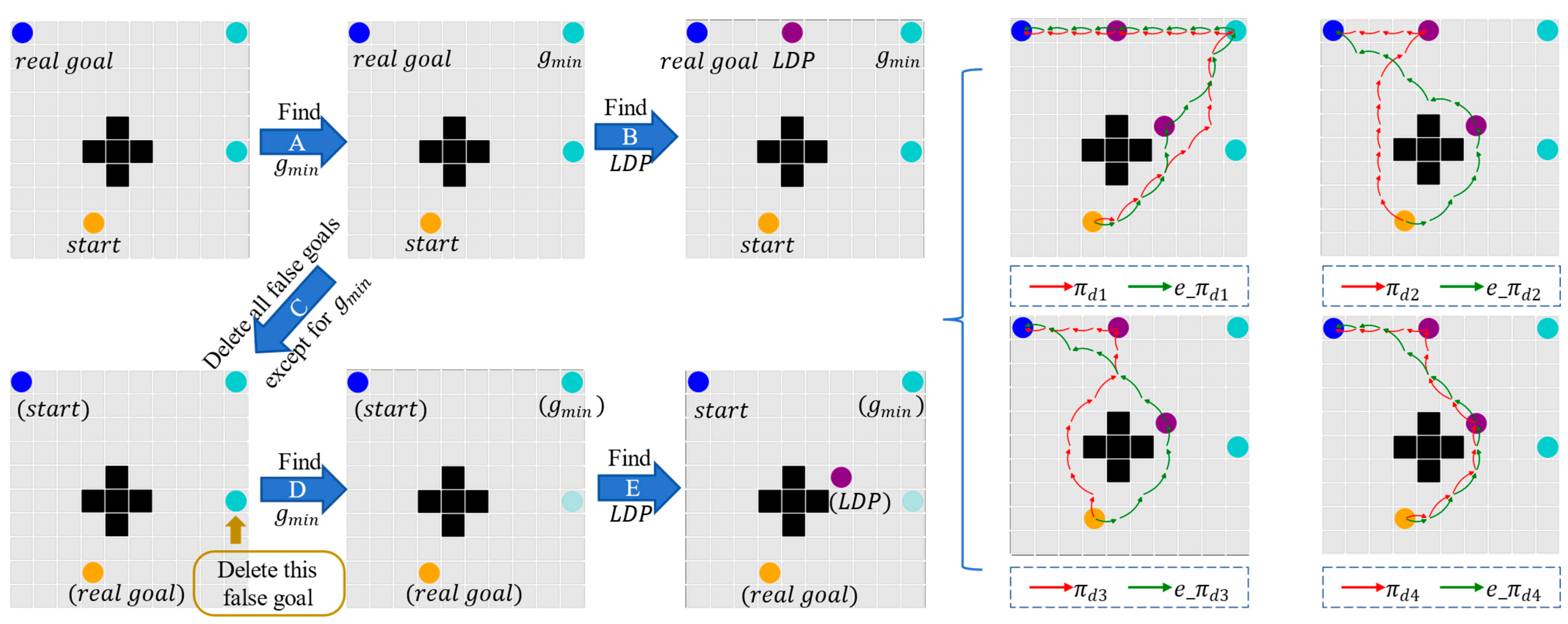
Firstly, , as detailed by Masters et al. [8], aim to maximize the Last Deceptive Point (LDP). The methods involve two main steps, as illustrated in the left half of Figure 2. Step A identifies gmin from the false goals, which is the most important false goal in the DPP problem, and Step B determines the LDP based on gmin. The paths planned by will be illustrated by the red arrows in the right half of Figure 2. Based on these, we introduce the as follows:
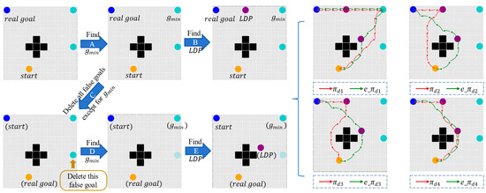
Figure 2.
The generation process of and for the original DPP problem is illustrated, where the orange dot represents the start point, the blue dot represents the real goal, teal dots denote the positions of false goals, and the purple dot indicates the location of LDP.
uses a “showing false” strategy where the observed navigates from the start point to gmin, and then continues to the real goal gr. The path generated by is a combination of two parts: . Similar to , focuses on identifying key node LDP on the optimal path from gmin to gr. Instead of navigating directly to gmin, it first heads towards LDP, then to gr. The path generated by is a combination of two parts: . Based on , also heads toward LDP first, but it introduces a modified heuristic approach biased toward the false goal gmin to increase the deceptive potential of the path. The path generated by is a combination of two parts: . utilizes a pre-computed probability “heatmap” to enhance path deception, significantly increasing the cost of to improve its deception. The path generated by is a combination of two parts: . In Figure 2, shows a clear tendency to approach the false goal gmin, indicating higher deception compared to with the same cost consumption. , although potentially less deceptive than in terms of deception level, it significantly reduces path duration compared to in the same DPP problem.
To further introduce methods, as depicted in the right half of Figure 2, the process of involves several steps. First, following Step A, once gmin is identified, Step C transforms the positions of “start” and “real goal”. Here, the original real goal becomes the new start point, and the original start point is designated as the new real goal. Simultaneously, all false goals except gmin are removed. This sets up a new DPP problem where the original real goal is the starting point, the original start point is the new real goal, and gmin remains as the sole false goal.
Building upon the new DPP problem, Step D identifies the new gmin (which, due to the deletions of other false goals, corresponds to gmin from the original path planning problem), followed by Step E to find the LDP for the new DPP problem. Subsequently, path planning proceeds based on . This approach yields four deceptive paths from “(start)” to “(real goal)” in Figure 2 based on this new path planning problem. These paths are then reversed to obtain four paths for the original deceptive path planning problem, as indicated by the green arrow on the right half of Figure 2.
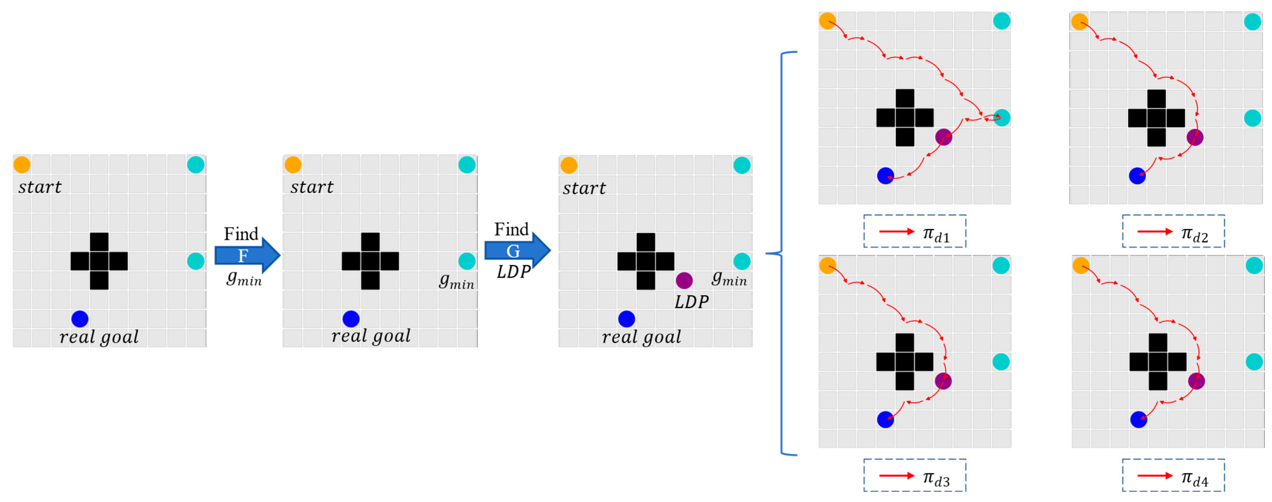
To facilitate further understanding of the differences between and , we also present the new DPP problem where additional false goals are not deleted in Figure 3. In contrast to the original DPP problem, in Figure 3, after Step A, gmin is different from the original DPP problem. Consequently, the LDP point also changes: from (6,5) in Figure 2 to (6,3) in Figure 3 (where the horizontal axis represents the x-coordinate and the vertical axis represents the y-coordinate, starting from 0). The resulting four paths generated by the method are depicted in the right half of Figure 3 as indicated by red arrows.
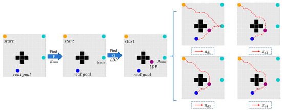
Figure 3.
The generation process of for the new DPP problem is illustrated, where the orange dot represents the start point, the blue dot represents the real goal, the teal dots denote the positions of false goals, and the purple dot indicates the location of LDP.
4.3. Deceptive Path Planning (DPP) via DPP_Q, Endpoint DPP_Q and LDP DPP_Q
We will provide a unified introduction to DPP_Q, Endpoint DPP_Q, and LDP DPP_Q. The core of these three methods is based on reinforcement learning modeling using Count-Based Q-learning. Below, we first introduce the state space, action space, and reward function of the observed as follows:
4.3.1. The State Space
The state space of the observed includes its current coordinate , as well as the number of straight and diagonal movements made by itself (denoted as and respectively). The state space S is defined as a four-dimensional vector:
4.3.2. The Action Space
The observed can take actions of two types: straight movements (up, down, left, right) and diagonal movements (up–left, down–left, up–right, down–right). The time required for straight movements is 1, while that of diagonal movements takes . Specifically, the action space is a matrix:
It means the observed has eight actions. Each of them was represented as a 4-dimensional vector corresponding to the state space S. The first two dimensions update the current coordinate of the observed (x, y), while the last two dimensions update the counts of straight and diagonal movements made by the observed. Given the state sT, the next state sT+1 can be obtained by simple vector addition:
i = 0, 1, 2, …, 7 represents the index of the action taken by the observed.
4.3.3. The Reward Function
Chen et al. [9] proposed an Approximate Goal Recognition Model (AGRM) based on PGRM and conducted comparative experiments using two different reward mechanisms, demonstrating the reliability of AGRM in computing rewards for the observed. Different from PGRM matching full of the observation sequence , the observer based on AGRM only matches the current node of the observed . Specifically, the formula for calculating the cost-difference is:
The formula for computing for each goal is as follows:
The observed is trained by AGRM. While training with PGRM is also feasible, AGRM allows for the advanced allocation of fuzzy rewards to each grid point, thereby circumventing the time-consuming reward computation during subsequent training in reinforcement learning. Specifically, assuming the current state sT of the observed, the formula for its basic reward is as follows:
where represents the current coordinate of the observed ncurrent, that is, .
We employed the count-based method to encourage the observed to explore unknown states. The count-based method can guide the observed to explore state-action pairs with higher uncertainty to confirm their high rewards. The uncertainty of the observed relative to its environment can be measured by [36], where is a constant and represents the number of times the state-action pair has been visited. Specifically, is set as an additional reward used to train the observed:
Intuitively, if the observed visited a state-action pair less frequently (i.e., is smaller), the corresponding additional reward will be larger. Thus it should be more inclined to visit this state-action pair to confirm whether it has a high reward. The rules for the observed to receive rewards are as follows:
- If the remaining time exceeds the shortest time the observed takes to reach the target, indicating it cannot arrive at the target within the time constraint. This scenario is denoted as Condition A, with a reward of −9 given.
- The observed successfully reaches the target, which is denoted as Condition B, with a reward of +100 given.
- Typically, the observed receives the deceptiveness of each grid point it traverses.
Specifically, the observed receives exploration rewards to encourage it to explore unknown state-action pairs. The reward function is shown as follows:
Below, we provide pseudocode for DPP_Q, Endpoint DPP_Q and LDP DPP_Q, using a 10 × 10 grid map as an example, accompanied by detailed explanations.
Algorithm 1 introduces the DPP problem and initializes it. It first sets up the learning rate, discount factor, and epsilon-greedy value, and initializes matrices D and Ds. D is a 10 × 10 matrix storing the shortest path lengths (equivalent to optimal time cost) from each grid point to the real goal gr. Ds is a 10 × 10 matrix storing the optimal time cost from each grid point to the start point s0. Furthermore, Algorithm 1 reads in various elements of the DPP problem: time constraints, obstacle coordinates, starting point coordinates, real goal coordinates, and coordinates of all fake goal points (line 1). Then, it initializes the Q-table and the counting matrix N-table, setting Q-values of illegal actions to −1000 (lines 2 to 3).
| Algorithm 1 DPP via Q-learning (Initialization and Problem Setup) |
. 1: Initialize distance matrix D and Ds, time constraint TC, collection of obstacle Wall, start node s0 resulting in the agent out of the map. |
Algorithm 2 describes the training process of the observed. First, the observed checks the legality of eight actions (lines 1 to 5). Then, the observed selects an action according to policy, and the state-action pairs are counted (lines 6 to 9). Subsequently, the observed receives a reward and updates the Q-table and the state (lines 10 to 13).
| Algorithm 2 DPP via Q learning (Training Framework) |
| 1:
2: 3: 4: : 7: 8: 9: |
Algorithm 3 describes the DPP_Q method. It first initializes the problem according to Algorithm 1. Then, it sets the initial start point of the observed as s0 and initializes its values for the next two dimensions to 0 (line 2). Each training round includes checking the termination condition: whether the remaining time exceeds the shortest observed time to reach the target (the real goal gr), indicating that the observed cannot reach the real goal within the time constraint , or the current coordinate of the observed coincide with the coordinate of the target (the real goal gr) scoord = gr (line 5). Finally, the optimal path can be collected using the method of tracking the maximum value of the Q-table (line 10).
| Algorithm 3 DPP_Q |
| Algorithm 1 2: 3: 4: Algorithm 2 5: 6: 7: 8: |
Algorithm 4 describes the Endpoint DPP_Q method. It first initializes the problem according to Algorithm 1. Then, it sets the initial exploration start point of the observed as the real goal gr, and initializes its values for the next two dimensions to 0 (line 2). Each training round includes checking the termination condition: whether the remaining time exceeds the shortest observed time to reach the start node s0, indicating that the observed cannot reach the real goal within the time constraint , or the current coordinate of the observed coincides with the coordinate of the target (the start node s0) scoord = s0. After collecting the path (line 10), performing a reversal operation yields a solution for the DPP problem (line 11).
| Algorithm 4 Endpoint DPP_Q |
| Algorithm 1 2: 3: 4: Algorithm 2 5: or scoord = s0: 6: break 7: end if 8: end while 9: end for 10: 11: ) |
Algorithm 5 describes the LDP DPP_Q method. It begins by initializing the problem according to Algorithm 1. Then, it computes the gmin to determine the coordinates of LDP, and calculatess the shortest cost distance from the LDP point to the false goal gmin: (line 1). The initial start point of the observed is set as LDP, with its values initialized to 0 for the next two dimensions (line 2). Subsequently, the algorithm divides into two steps that can be executed in parallel or sequentially: one agent starts from LDP to explore paths that can reach the real goal gr within the time constraint , while another agent starts from LDP to explore paths that can reach the start node s0 within the time constraint . After collecting the paths, performing a reversal and concatenation operation yields a solution for the DPP problem starting from s0 and ending at gr (line 21).
| Algorithm 5 LDP DPP_Q |
| Algorithm 1 3: 4: while True: 5: Algorithm 2 7: break 15: Algorithm 2 or scoord = s0: |
5. Experiments and Results
We divided the experiments into three parts. Firstly, we randomly generated a total of 300 DPP problems based on 10 × 10 grid maps to verify the effectiveness comparison between and . Next, we also randomly generated a total of 300 DPP problems based on 10 × 10 grid maps to validate the effectiveness of DPP_Q, Endpoint DPP_Q, and LDP DPP_Q. Finally, we used large maps from Moving-AI to further verify the effectiveness of DPP_Q, Endpoint DPP_Q and LDP DPP_Q.
5.1. Performance Evaluation of (Compared with )
5.1.1. Experimental Design
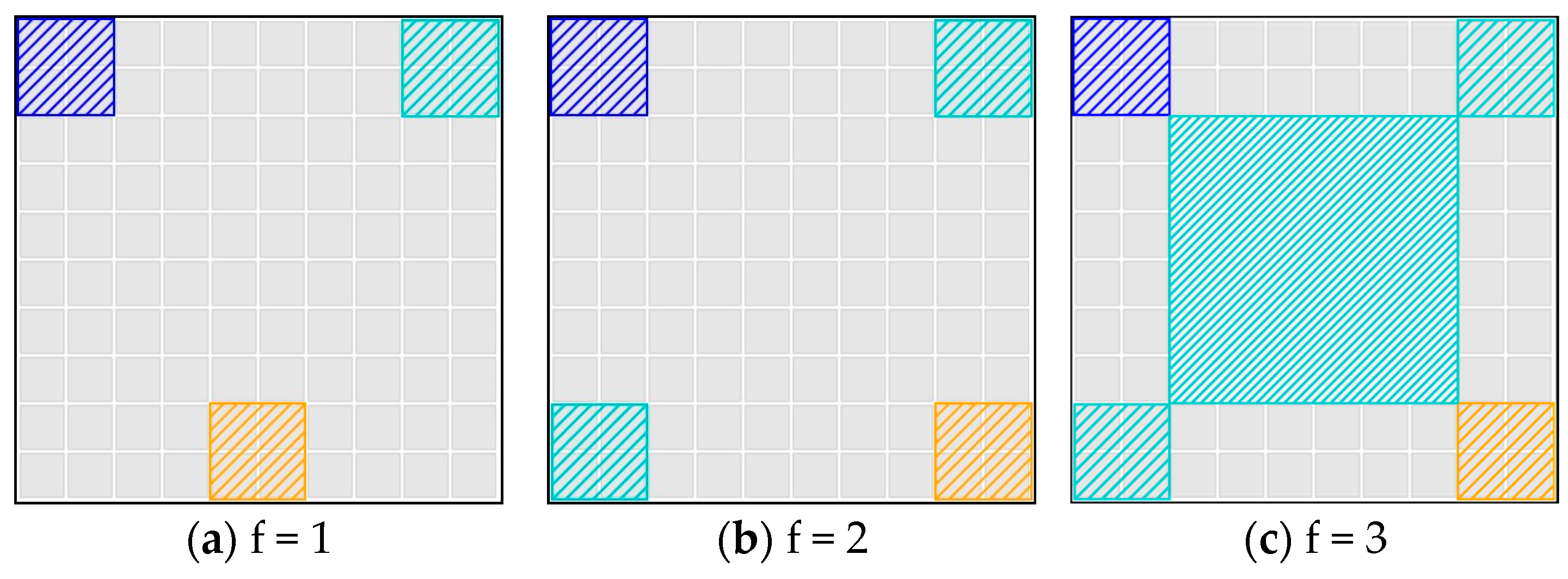
Considering the need to collect sufficient experimental data to ensure the reliability of performance testing results, we investigated the scenarios with 1, 2, and 3 false goals. The experiments were conducted on 300 10 × 10 grid maps, each randomly populated with 4 to 9 obstacle grid cells. For the case with one false goal, we generated 100 maps where one start node was randomly placed in the lower-middle area, one real goalwas randomly located in the upper-left corner and one false goal was randomly positioned in the upper-right corner (as shown in Figure 4a). For the case with two false goals, another set of 100 maps was generated where one start node was randomly placed in the bottom-right corner, one real goal was randomly placed in the upper-left corner and two false goals were randomly placed in the upper-right and lower-left corners respectively (as shown in Figure 4b). For the scenario with three false goals, building upon the distribution seen in Figure 4b for two false goals, we randomly added a third false goal positioned in the middle area (as illustrated in Figure 4c). This experimental design emphasizes the unique characteristics of DPP problems when there is a certain distance between the start node, real goal, and false goals.
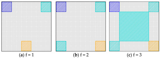
Figure 4.
Key grid points randomly generated for DPP problems. Here, the orange region denotes the area where start nodes are generated, the blue region represents the area where real goals are generated, and the teal region indicates the area for false goals.
5.1.2. Experimental Results
As shown in Figure 5, we randomly select one map each for the experiments with 1, 2, and 3 false goals to demonstrate the results. Here, f denotes the number of false goals. In Figure 5, the black squares represent obstacles, the orange dot represents the start point, the blue dot represents the real goal, the teal dots denote the positions of false goals, the red arrows indicate the path, and the green arrows represent the path.
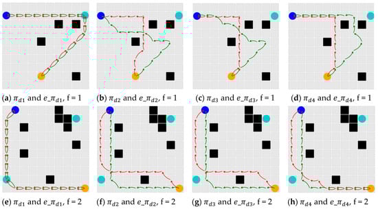
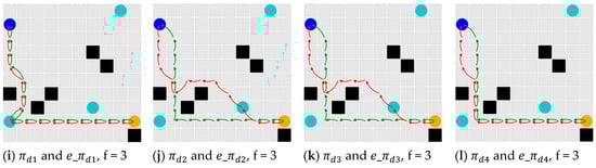
Figure 5.
Comparison of deceptive paths generated by and .
Table 1 demonstrates a significant difference in the ADI of paths generated by compared to . The improvements of over traditional are substantial. Experimentally, shows almost no improvement compared to (−0.03%), while averages an improvement of 16.83% compared with , averages an improvement of 10.47% compared with , and averages an improvement of 5.03% compared with . Overall, shows an average improvement of 8.07% over .

Table 1.
The five-number summary describes the improvements of ADI of paths generated by compared with , where .
For and , their performances are nearly indistinguishable. However, for and , the improvements are quite significant. Of course, this also relates to the distribution of true and false goals. Although Table 1 suggests that the advantage of is less pronounced when there are three false goals compared to 1 or 2; this may be due to the specific placement of the third false goal, which is close to both the start node and the real goal. If the third false target were also randomly placed in a corner position, the advantage of would likely be more pronounced.
5.2. Performance Evaluation of Endpoint DPP_Q and LDP DPP_Q (Compared with DPP_Q)
In this section, we first conduct batch experiments on 10 × 10 maps to verify the advantages of Endpoint DPP_Q and LDP DPP_Q over the baseline DPP_Q. Subsequently, we perform further tests on 49 × 49 maps based on the Moving-AI benchmark.
5.2.1. Experimental Design
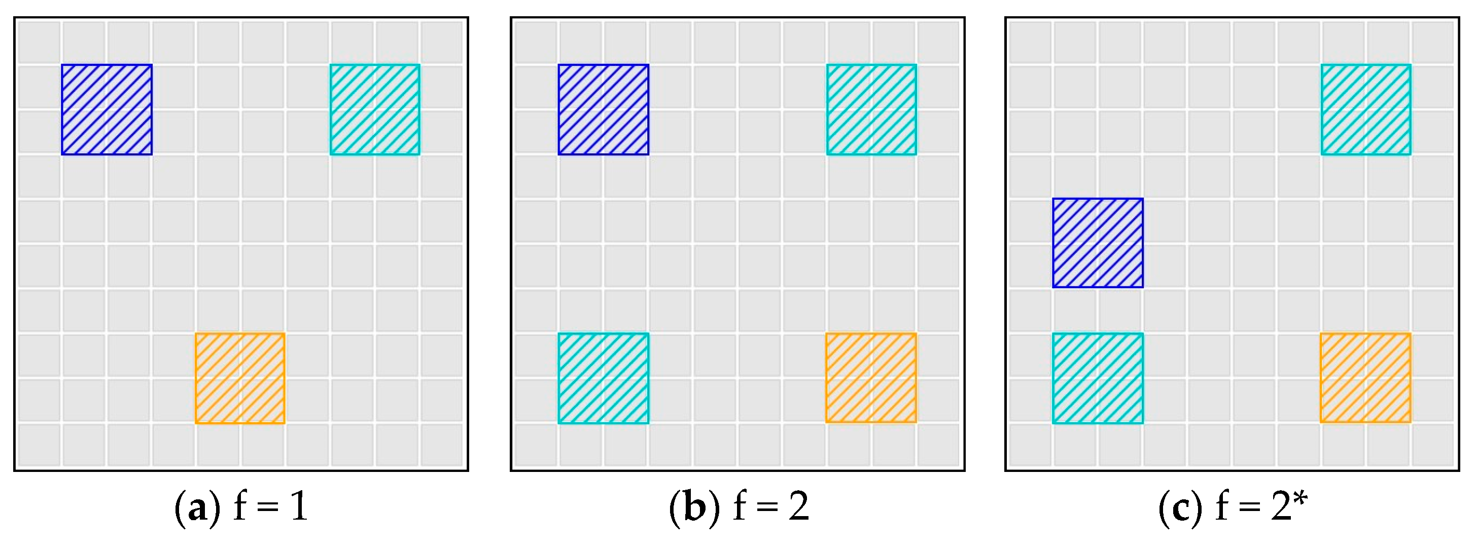
Considering the need for sufficient experimental data to ensure the reliability of performance testing for DPP_Q, Endpoint DPP_Q and LDP DPP_Q, we conducted experiments on 300 10 × 10 grid maps. Each map contained randomly generated obstacle grids (4 to 9) following the methodology in Section 5.1. We investigated scenarios with one or two false goals. For maps with one false goal, we randomly placed one start node in the lower-middle area, one real goal in the upper-left corner and one false goal in the upper-right corner (as in Figure 6a), across 100 maps. For scenarios with two false goals, firstly, regarding the symmetric distribution, we randomly placed one start node in the lower-right corner, one real goal in the upper-left corner and two false goals in the upper-right and lower-left corners respectively (Figure 6b). There were also 100 maps generated of this type. For the asymmetric distribution, the position of the real goal varied (Figure 6c), and 100 maps were generated. The * symbol indicates maps with special distributions of real and false goals. These experiments aimed to thoroughly evaluate how these configurations impact the performance of our methods under various conditions.
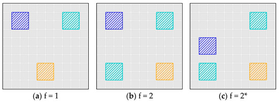
Figure 6.
Key grid points randomly generated for DPP problems. Here, the orange region denotes the area where start nodes are generated, the blue region represents the area where real goals are generated, and the teal region indicates the area for false goals.
For the methods used here—time-constrained DPP_Q, Endpoint DPP_Q, and LDP DPP_Q—we aimed to make the experiments more realistic and feasible. For each set of experiments (f = 1, f = 2, and f = 2*), consisting of 100 maps, we employed the method to generate 100 deceptive paths. We then selected the maximum time cost from these paths, rounded up to the nearest integer, to serve as the time constraints for our experiments. Specifically, for f = 1, the time constraint was set to 15 (derived from a rounded-up maximum of 14.242); for f = 2, the time constraint was set to 16 (rounded up from 15.414) and for f = 2*, the time constraint was set to 13 (rounded up from 12.242).
The choice of was deliberate because it provides paths with moderate time consumption and generally higher deception levels on average, making it a notable method within traditional approaches. Of course, any other time constraints could be used as long as all path-planning problems under these constraints have feasible solutions.
5.2.2. Experimental Results
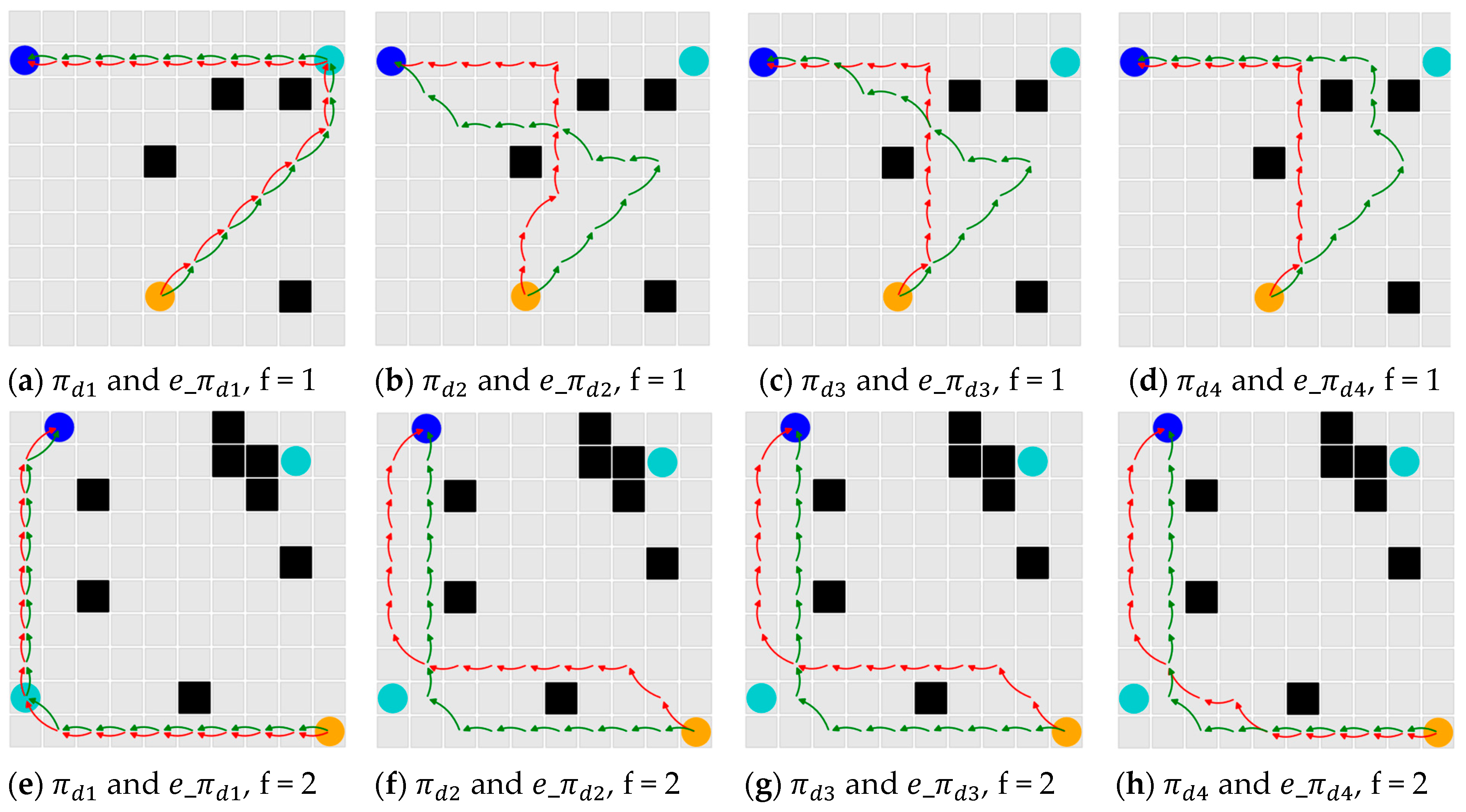
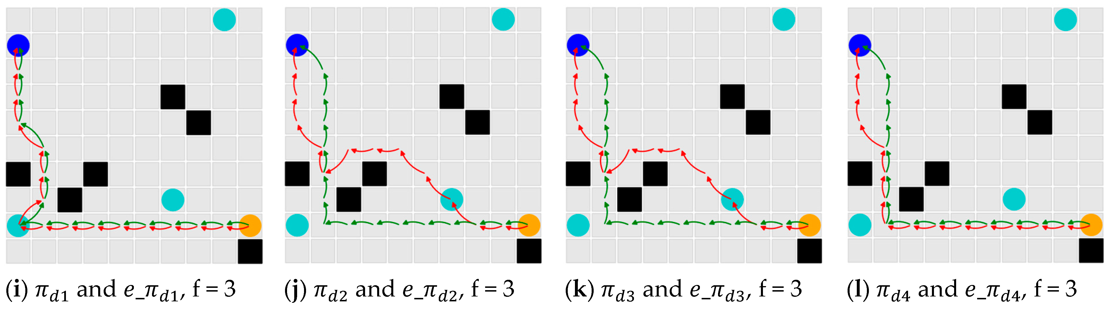
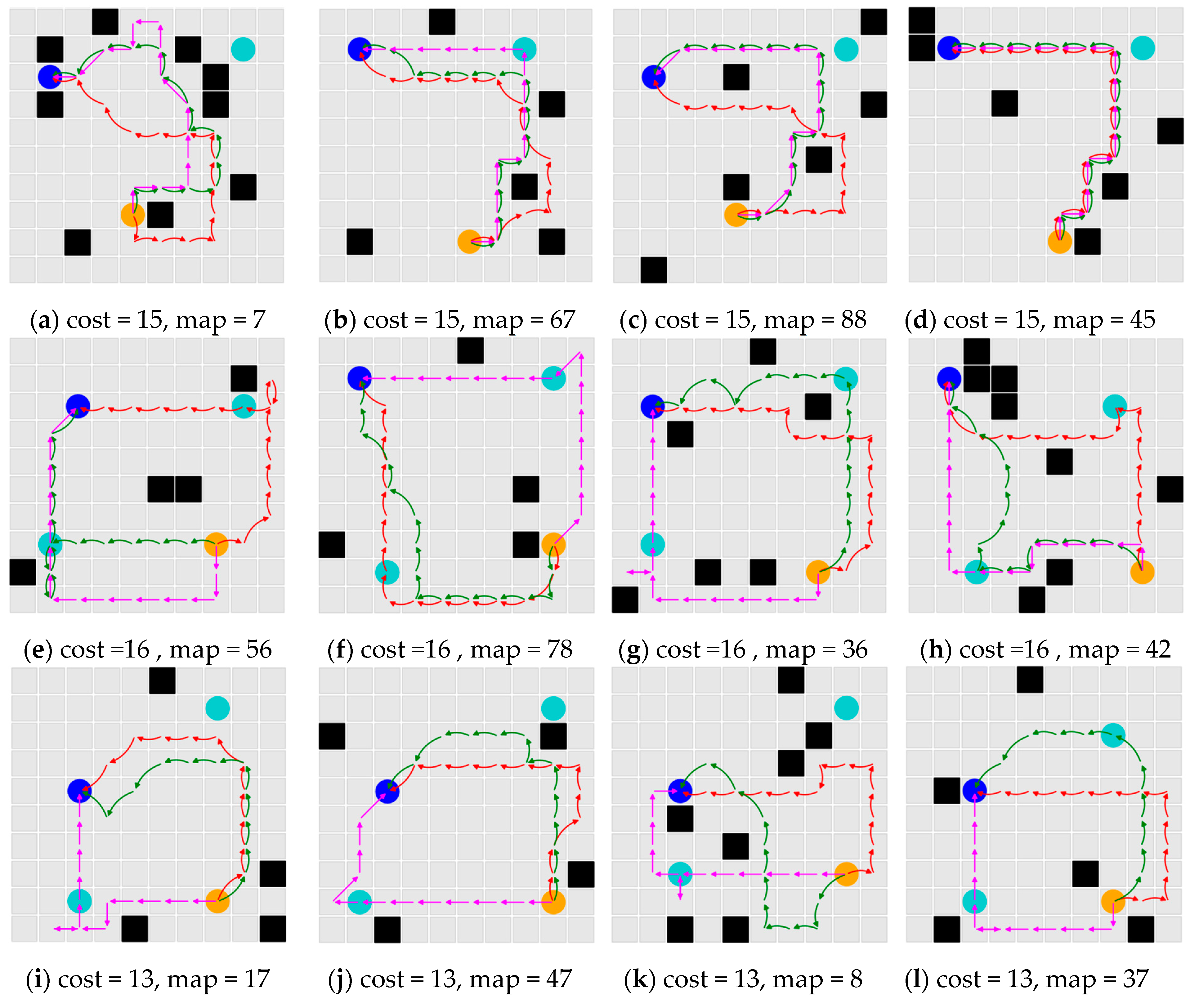
For illustration, we randomly selected four maps from each of the three types of DPP problems mentioned above. Figure 7a–d display the paths generated by DPP_Q, Endpoint DPP_Q, and LDP DPP_Q for four random maps from the f = 1 group. Figure 7e–h correspond to four random maps from the f = 2 group, and Figure 7i–l depict four random maps from the f = 2* group. In these figures, paths generated by DPP_Q are indicated by red arrows, paths by Endpoint DPP_Q are indicated by green arrows, and paths by LDP DPP_Q are indicated by magenta arrows, and the black squares represent obstacles, the orange dot represents the start point, the blue dot represents the real goal, the teal dots denote the positions of false goals. The term “cost” denotes the specific time constraint used for path planning, and “map” indicates the map number selected from the 100 maps available. There are notable differences in the paths generated by DPP_Q, Endpoint DPP_Q, and LDP DPP_Q.

Figure 7.
Comparison of deceptive paths generated by DPP_Q, Endpoint DPP_Q and LDP DPP_Q.
From Table 2, it can be observed that the differences between the new and old methods are not significant (less than 1%) when f = 1 and f = 2. However, when f = 2*, the relative effectiveness of Endpoint DPP_Q and LDP DPP_Q compared to DPP_Q becomes more pronounced (approximately 2.7%). These results are based on a 10 × 10 small-scale map.
Table 2.
The five-number summary describes the improvements of ADI of paths generated by Endpoint DPP_Q and LDP DPP_Q, compared with DPP_Q, where . represents paths generated by DPP_Q, represents paths generated by Endpoint DPP_Q, and represents paths generated by LDP DPP_Q.
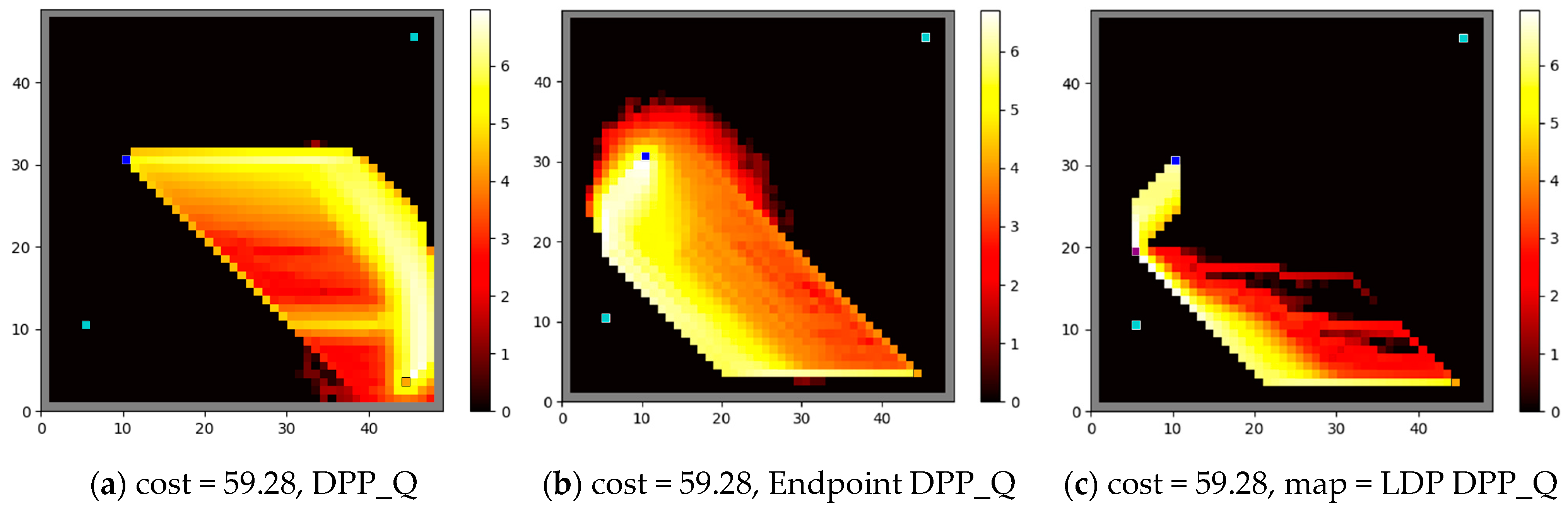
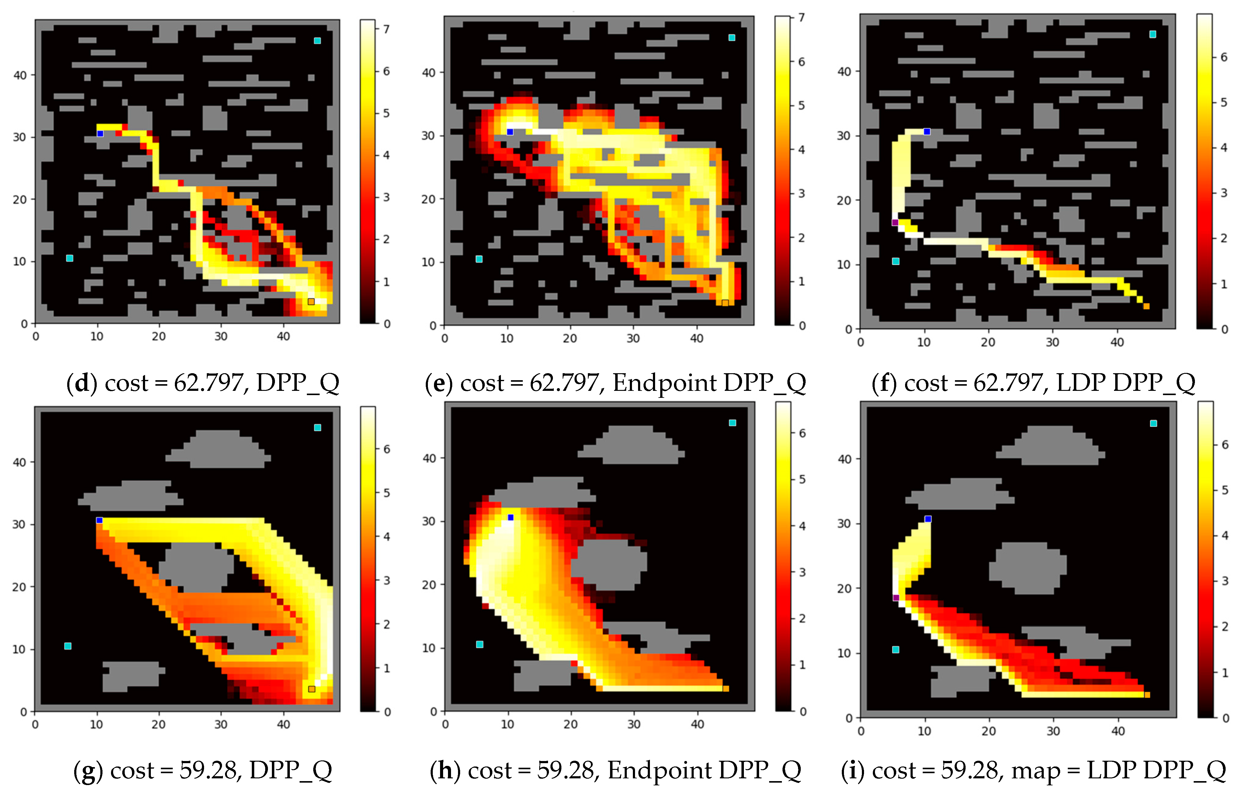
Below, we conduct experiments on the classic 49 × 49 large maps from Moving-AI, specifically using the maps called “49_empty.map”, “49_small.map”, and “49_large.map”. The start point coordinates are set to (44, 3), with the real goal located at (10, 30). There are two false goals located at (5, 10) and (45, 45), respectively.
Figure 8 displays heatmaps of the exploration of each grid point after training for 10,000,000 iterations. The color bars on the right of each image represent logarithmically scaled values (base 10). The “cost” refers to the time constraints given to the observed, resulting in time costs of 59.28, 62.797, and 59.28 for the DPP problems solved using on “49_empty.map”, “49_small.map”, and “49_large.map”, respectively. The orange squares (black borders) denote the start point, the blue squares (white borders) denote the real goal, and the teal squares (white borders) denote the locations of the false goals. In Figure 8c,f,i, the purple squares (white borders) indicate the coordinates of the LDP points corresponding to the respective DPP problems.
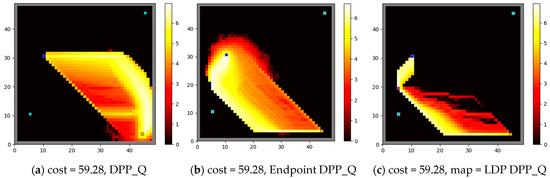

Figure 8.
Display of the observed exploration heatmap, trained by DPP_Q, Endpoint DPP_Q, and LDP DPP_Q in 49 × 49 maps.
Figure 8a–c show the exploration patterns of the observed for DPP_Q, Endpoint DPP_Q, and LDP DPP_Q in the “49_empty.map” scenario. Figure 8d–f depict the exploration in the “49_small.map” scenario, while Figure 8g–i display the exploration in the “49_large.map” scenario. Figure 8b,e,h reveal that Endpoint DPP_Q effectively addresses the initial issue of DPP_Q, as shown in Figure 8a,d, and g, where it often gets stuck in local optima early on. Further analysis of Figure 8c,f,i shows that LDP DPP_Q not only resolves the initial local optima problem seen in Figure 8a,d,g but also reduces the exploration space intelligently, potentially speeding up the training process.
Figure 9a,c,e depict heatmaps of reward functions for the three DPP problems. The red, green, and magenta lines represent paths generated by DPP_Q, Endpoint DPP_Q, and LDP DPP_Q, respectively. Similar to Figure 8, the orange squares (black borders) denote the start point, blue squares (white borders) denote the real goal, and teal squares (white borders) denote the false goals. The purple squares (white borders) in Figure 9a,c,e represent the coordinates of LDP of the relative DPP problems.
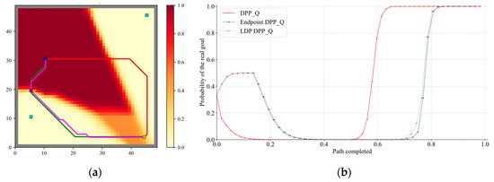
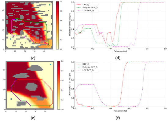
Figure 9.
Comparison of deceptive paths generated by DPP_Q, Endpoint DPP_Q and LDP DPP_Q in 49 × 49 maps.
In Figure 9b,d,f, the x-axis represents the progress along the path (ranging from 0 to 1), while the y-axis represents the posterior probability of the real goal. The red, green, and magenta lines illustrate how the posterior probability of the real goal changes in the path generated by DPP_Q, Endpoint DPP_Q, and LDP DPP_Q, respectively. It is observed that the red line tends to reach around 1.0 earlier than the green and magenta lines in Figure 9b. In Figure 9b, the green and magenta lines almost overlap (with ADD of 0.586 for DPP_Q, 0.703 for Endpoint DPP_Q, and 0.695 for LDP DPP_Q), while in Figure 9d, LDP DPP_Q notably outperforms Endpoint DPP_Q and DPP_Q (with ADD of 0.316 for DPP_Q, 0.423 for Endpoint DPP_Q, and 0.558 for LDP DPP_Q). Figure 9e shows even closer alignment between the green and magenta lines (mean deception scores of 0.530 for DPP_Q, 0.635 for Endpoint DPP_Q, and 0.635 for LDP DPP_Q), demonstrating that LDP DPP_Q effectively enhances ADD, similar to Endpoint DPP_Q. Given the same time constraints, using ADD as a metric provides a more intuitive comparison of the three path-planning strategies.
6. Discussion and Conclusions
In this paper, we introduce two metrics for measuring the solutions of DPP problems: ADD and ADI. Employing a reverse-thinking approach, we propose three new methods (, Endpoint DPP_Q and LDP DPP_Q) that demonstrate significant improvements compared to the original methods ( and DPP_Q).
Firstly, we define the concept of ADD. Based on ADD, we further develop the notion of ADI and analyze its validity, applying it to evaluate subsequent methods. Secondly, we enhance without time constraints by introducing , which shows substantial improvements over traditional methods. Experimental results indicate negligible improvement for compared with (−0.03%), a significant average improvement of 16.83% for compared with , a 10.47% average improvement for compared with , and a 5.03% average improvement for compared with . Overall, outperforms by 8.07%. Finally, addressing methods under time constraints like DPP_Q, we propose Endpoint DPP_Q and LDP DPP_Q. Both methods effectively address the issue of poor path deception in DPP_Q when the real and false goals have specific distributions. Moreover, Endpoint DPP_Q and LDP DPP_Q demonstrate even more significant advantages in overcoming local optima issues on large maps compared to DPP_Q, resulting in substantial improvements.
For future work, we recognize that the training times of methods such as DPP_Q, Endpoint DPP_Q, and LDP DPP_Q are still lengthy. Inspired by the principles of , we suggest segmenting paths by incorporating more navigation points that are similar to LDP. Segmenting agent training could accelerate learning while achieving comparable results. Additionally, modeling the goal recognition method of the observer remains challenging. PGRM serves as an assumption model that is potentially inaccurate or flawed. Future research should introduce adversarial elements and more complex opponent goal recognition models. For example, the observed may quickly perceive the identifications or actions of the observer and adjust their planning accordingly to enhance deception strategies. Furthermore, expanding DPP problems to higher dimensions, such as three-dimensional space for drone flight or dynamic environments, promises practical advancements. Incorporating additional elements like images or audio captured by identifiers rather than solely relying on coordinates could make the game more intricate. These directions hold promise for future research, enhancing practical applicability significantly.
Author Contributions
Conceptualization, D.C. and K.X.; methodology, D.C.; validation, D.C. and Q.Y.; formal analysis, D.C.; investigation, D.C.; data curation, D.C.; writing—original draft preparation, D.C.; writing—review and editing, D.C.; supervision, Q.Y. and K.X.; funding acquisition, K.X. All authors have read and agreed to the published version of the manuscript.
Funding
This work was supported by the Natural Science Foundation of China (grant number 62103420).
Data Availability Statement
No new data were created or analyzed in this study. Data sharing is not applicable to this article.
Acknowledgments
We thank Peta Masters and Sebastian Sardina of RMIT University for their support with the open-source code. Deceptive Path-Planning algorithms can be found at GitHub—ssardina-planning/p4-simulator: Python Path Planning Project (P4) (https://github.com/ssardina-planning/p4-simulator) (accessed on 17 June 2024).
Conflicts of Interest
The authors declare no conflicts of interest.
Correction Statement
This article has been republished with a minor correction to resolve spelling. This change does not affect the scientific content of the article.
Abbreviations
The following abbreviations are used in this manuscript:
| DPP | Deceptive path planning |
| ADD | Average Deception Degree |
| ADI | Average Deception Intensity |
| LDP | Last Deceptive Point |
| AHMM | Abstract Hidden Markov Models |
| PGRM | Precise Goal Recognition Model |
| AGRM | Approximate Goal Recognition Model |
References
- Alloway, T.P.; McCallum, F.; Alloway, R.G.; Hoicka, E. Liar, liar, working memory on fire: Investigating the role of working memory in childhood verbal deception. J. Exp. Child Psychol. 2015, 137, 30–38. [Google Scholar] [CrossRef] [PubMed]
- Greenberg, I. The effect of deception on optimal decisions. Oper. Res. Lett. 1982, 1, 144–147. [Google Scholar] [CrossRef]
- Matsubara, S.; Yokoo, M. Negotiations with inaccurate payoff values. In Proceedings of the International Conference on Multi Agent Systems (Cat. No. 98EX160), Paris, France, 3–7 July 1998; pp. 449–450. [Google Scholar]
- Shieh, E.; An, B.; Yang, R.; Tambe, M.; Baldwin, C.; DiRenzo, J.; Maule, B.; Meyer, G. Protect: A deployed game theoretic system to protect the ports of the united states. In Proceedings of the 11th International Conference on Autonomous Agents and Multiagent Systems, Valencia, Spain, 4–8 June 2012; Volume 1, pp. 13–20. [Google Scholar]
- Geib, C.W.; Goldman, R.P. Plan recognition in intrusion detection systems. In Proceedings of the DARPA Information Survivability Conference and Exposition II, DISCEX’01, Anaheim, CA, USA, 12–14 June 2001; pp. 46–55. [Google Scholar]
- Kitano, H.; Asada, M.; Kuniyoshi, Y.; Noda, I.; Osawa, E. Robocup: The robot world cup initiative. In Proceedings of the First International Conference on Autonomous Agents, Marina Del Rey, CA, USA, 5–8 February 1997; pp. 340–347. [Google Scholar]
- Keren, S.; Gal, A.; Karpas, E. Privacy Preserving Plans in Partially Observable Environments. In Proceedings of the IJCAI, New York, NY, USA, 9–15 July 2016; pp. 3170–3176. [Google Scholar]
- Masters, P.; Sardina, S. Deceptive Path-Planning. In Proceedings of the IJCAI, Melbourne, Australia, 19–25 August 2017; pp. 4368–4375. [Google Scholar]
- Chen, D.; Zeng, Y.; Zhang, Y.; Li, S.; Xu, K.; Yin, Q. Deceptive Path Planning via Count-Based Reinforcement Learning under Specific Time Constraint. Mathematics 2024, 12, 1979. [Google Scholar] [CrossRef]
- Avrahami-Zilberbrand, D.; Kaminka, G.A. Incorporating observer biases in keyhole plan recognition (efficiently!). In Proceedings of the AAAI, Melbourne, Australia, 19–25 August 2007; pp. 944–949. [Google Scholar]
- Nichols, H.; Jimenez, M.; Goddard, Z.; Sparapany, M.; Boots, B.; Mazumdar, A. Adversarial sampling-based motion planning. IEEE Robot. Autom. Lett. 2022, 7, 4267–4274. [Google Scholar] [CrossRef]
- Cohen, P.R.; Perrault, C.R.; Allen, J.F. Beyond question answering. In Strategies for Natural Language Processing; Psychology Press: London, UK, 2014; pp. 245–274. [Google Scholar]
- Kautz, H.A.; Allen, J.F. Generalized plan recognition. In Proceedings of the AAAI, Philadelphia, PA, USA, 11–15 August 1986; p. 5. [Google Scholar]
- Pynadath, D.V.; Wellman, M.P. Generalized queries on probabilistic context-free grammars. IEEE Trans. Pattern Anal. Mach. Intell. 1998, 20, 65–77. [Google Scholar] [CrossRef]
- Pynadath, D.V. Probabilistic Grammars for Plan Recognition; University of Michigan: Ann Arbor, MI, USA, 1999. [Google Scholar]
- Pynadath, D.V.; Wellman, M.P. Probabilistic state-dependent grammars for plan recognition. arXiv 2013, arXiv:1301.3888. preprint. [Google Scholar]
- Geib, C.W.; Goldman, R.P. A probabilistic plan recognition algorithm based on plan tree grammars. Artif. Intell. 2009, 173, 1101–1132. [Google Scholar] [CrossRef]
- Bui, H.H. A general model for online probabilistic plan recognition. In Proceedings of the IJCAI, Acapulco, Mexico, 9–15 August 2003; pp. 1309–1315. [Google Scholar]
- Liao, L.; Patterson, D.J.; Fox, D.; Kautz, H. Learning and inferring transportation routines. Artif. Intell. 2007, 171, 311–331. [Google Scholar] [CrossRef]
- Ramírez, M.; Geffner, H. Probabilistic plan recognition using off-the-shelf classical planners. In Proceedings of the AAAI Conference on Artificial Intelligence, Atlanta, GA, USA, 11–15 July 2010; pp. 1121–1126. [Google Scholar]
- Sohrabi, S.; Riabov, A.V.; Udrea, O. Plan Recognition as Planning Revisited. In Proceedings of the IJCAI, New York, NY, USA, 9–15 July 2016; pp. 3258–3264. [Google Scholar]
- Bui, H.H.; Venkatesh, S.; West, G. Policy recognition in the abstract hidden markov model. J. Artif. Intell. Res. 2002, 17, 451–499. [Google Scholar] [CrossRef]
- Ramırez, M.; Geffner, H. Plan recognition as planning. In Proceedings of the 21st International Joint Conference on Artifical Intelligence, Pasadena, CA, USA, 11–17 July 2009; Morgan Kaufmann Publishers Inc.: Cambridge, MA, USA, 2009; pp. 1778–1783. [Google Scholar]
- Masters, P.; Sardina, S. Cost-based goal recognition for path-planning. In Proceedings of the 16th Conference on Autonomous Agents and Multiagent Systems, São Paulo, Brazil, 8–12 May 2017; pp. 750–758. [Google Scholar]
- Floridi, L. The Philosophy of Information; Oxford University Press: Oxford, UK, 2011. [Google Scholar]
- Fetzer, J.H. Disinformation: The use of false information. Minds Mach. 2004, 14, 231–240. [Google Scholar] [CrossRef]
- Fallis, D. What is disinformation? Libr. Trends 2015, 63, 401–426. [Google Scholar] [CrossRef]
- Sarkadi, S.; Wright, B.; Masters, P.; McBurney, P. Deceptive AI; Springer: Berlin/Heidelberg, Germany, 2021. [Google Scholar]
- Bell, J.B. Toward a theory of deception. Int. J. Intell. Counterintell. 2003, 16, 244–279. [Google Scholar] [CrossRef]
- Arkin, R.C.; Ulam, P.; Wagner, A.R. Moral decision making in autonomous systems: Enforcement, moral emotions, dignity, trust, and deception. Proc. IEEE 2011, 100, 571–589. [Google Scholar] [CrossRef]
- Cai, Z.; Ju, R.; Zeng, Y.; Xie, X. Deceptive Path Planning in Dynamic Environment. In Proceedings of the 2020 3rd International Conference on Advanced Electronic Materials, Computers and Software Engineering (AEMCSE), Shenzhen, China, 24–26 April 2020; pp. 203–207. [Google Scholar]
- Xu, K.; Zeng, Y.; Qin, L.; Yin, Q. Single real goal, magnitude-based deceptive path-planning. Entropy 2020, 22, 88. [Google Scholar] [CrossRef] [PubMed]
- Liu, Z.; Yang, Y.; Miller, T.; Masters, P. Deceptive reinforcement learning for privacy-preserving planning. arXiv 2021, arXiv:2102.03022. [Google Scholar]
- Lewis, A.; Miller, T. Deceptive reinforcement learning in model-free domains. In Proceedings of the International Conference on Automated Planning and Scheduling, Prague, Czech Republic, 8–13 July 2023; pp. 587–595. [Google Scholar]
- Hart, P.E.; Nilsson, N.J.; Raphael, B. A formal basis for the heuristic determination of minimum cost paths. IEEE Trans. Syst. Sci. Cybern. 1968, 4, 100–107. [Google Scholar] [CrossRef]
- Strehl, A.L.; Littman, M.L. An analysis of model-based interval estimation for Markov decision processes. J. Comput. Syst. Sci. 2008, 74, 1309–1331. [Google Scholar] [CrossRef]


Disclaimer/Publisher’s Note: The statements, opinions and data contained in all publications are solely those of the individual author(s) and contributor(s) and not of MDPI and/or the editor(s). MDPI and/or the editor(s) disclaim responsibility for any injury to people or property resulting from any ideas, methods, instructions or products referred to in the content. |
© 2024 by the authors. Licensee MDPI, Basel, Switzerland. This article is an open access article distributed under the terms and conditions of the Creative Commons Attribution (CC BY) license (https://creativecommons.org/licenses/by/4.0/).