Article

Process Capability Index for Simple Linear Profile in the Presence of Within- and Between-Profile Autocorrelation

1
Department of Industrial Engineering, Kosar University of Bojnord, Bojnord 9453155168, Iran
2
Department of Mathematical Statistics and Actuarial Science, Faculty of Natural and Agricultural Sciences, University of the Free State, Bloemfontein 9301, South Africa
3
Information Systems and Operations Management Department, College of Business, University of Central Oklahoma, Edmond, OK 73034, USA
*
Author to whom correspondence should be addressed.
Mathematics 2024, 12(16), 2549; https://doi.org/10.3390/math12162549
Submission received: 17 July 2024 / Revised: 14 August 2024 / Accepted: 15 August 2024 / Published: 18 August 2024

Abstract

:
In many situations, the quality of a process or product can be characterized by a functional relationship or profile. It is well-known that the independence assumptions of the error terms within or between profiles are not always valid and could be violated due to within or between profile autocorrelation. Since most of the process capability indices (PCIs) have been developed for simple linear profiles (SLPs) without considering autocorrelation, this paper provides some novel methods to analyze the capability of SLP under each of the two different autocorrelation effects separately, as well as the case where both autocorrelation effects are present. We assume that the first-order autoregressive AR(1) model explains the within- and between-profile autocorrelation in error terms. To evaluate the process capability, a new functional index called C p ( P r o f i l e ) is introduced for SLP with independent errors, and then it is modified to include the three possible cases of within, between, and simultaneous autocorrelation. The simulation results demonstrate that the proposed schemes outperform existing schemes regarding bias and mean square error (MSE) criteria. Moreover, bootstrap confidence intervals for the proposed index are obtained. Finally, an illustrative example in the chemical industry is used to demonstrate the applicability of the proposed method.

1. Introduction

A control chart, as a featured tool of statistical process control (SPC), can be used to monitor a single or a vector of quality characteristics with the aim of improving manufacturing and service processes. In some applications, a functional relationship between a response and one or more explanatory variables could represent the quality of such processes effectively. This functional relationship, which is referred to as a profile, can be linear or nonlinear in nature. In the simplest but most fundamental case, a simple linear profile (SLP) represents a response variable as a function of a single explanatory variable [1]. In the related literature, several methods have been developed for monitoring simple linear profiles in Phase I and Phase II of control charts. As a pioneering work, Kang and Albin [2] developed a method to monitor SLP in Phase II using Hoteling T 2 and exponentially weighted moving average (EWMA) control charts. They showed that EWMA was a proper choice for detecting small and moderate shifts, while Hoteling T 2 performed well in detecting large shifts. Due to the remarkable performance of the EWMA scheme, some other researchers, including Kim et al. [3] and Li and Wang [4] developed several other monitoring schemes based on the EWMA control chart. Moreover, other ideas, including the implementation of the generalized likelihood ratio method [5], deep learning structures [6], and robust estimators [7] have been proposed to improve the efficiency of control charts in SLP monitoring. For more details on profile monitoring, interested readers are referred to the literature review done by Maleki et al. [8].
In most of the methods developed in the literature for profile monitoring, it is assumed that profiles are independent over time. This assumption can be easily violated in some processes where quality characteristics of interest from different samples collected over time are autocorrelated. It is well known that when methods such as those discussed above are applied to processes where autocorrelation is an inherent part of the process, one should expect misleading results due to errors in parameter estimation. Generally, we consider two types of autocorrelations in profile monitoring, namely between profile autocorrelation (BPAC) and within profile autocorrelation (WPAC). Between profile autocorrelation (BPAC) refers to the case where observations on each profile are related to each other via a specific autocorrelation model over time. For example, Noorossana et al. [9] assumed a first order autoregressive model AR(1) for profile observations and extended T 2 and EWMA control charts to monitor SLP. In this approach, a proper transformation of the response variables was applied to reach an independent profile model. To improve the detection ability of the EWMA scheme, Wang and Huang [10] suggested a more efficient statistic to remove the autocorrelation from the residuals. Some other ideas, such as U statistics [11] and multivariate EWMA [12], were also proposed for the elimination of BPAC. On the other hand, the within profile autocorrelation (WPAC) was considered in the second group. It was followed by a model in which the observations of each profile depend on each other under an autocorrelation effect. As a pioneering work, Soleimani et al. [13] first reduced the dimension of profile samples, and then four control charts were proposed to monitor the responses and residuals. They compared T 2 and EWMA control charts under the WPAC, and they concluded that EWMA based methods could detect small shifts faster. Jensen et al. [14] and Zhang et al. [15] proposed robust control charts to counteract the autocorrelation effect. Moreover, other methods such as principal component analysis and support vector machines were also developed to monitor profiles with WPAC [16,17]. Recently, Nadi et al. [18] considered SLPs with both between and within autocorrelation effects. We use BAC abbreviation to refer to the case when BPAC and WPAC occur in a profile simultaneously. Considering the studies by Noorossana et al. [9] and Soleimani et al. [13], Nadi et al. [18] introduced and compared four control charts for monitoring SLP processes with BAC effects.
When a process is under statistical control, one needs to evaluate process performance via process capability analysis (PCA). Process capacity indices (PCIs) provide a quantitative measure using specification limits (SLs) to identify capable processes. Generally, larger PCI values indicate a more capable process. PCA has been conducted for both monitoring quality characteristics [19,20,21,22] and different profile types [23,24,25]. The traditional PCA is conducted under the assumption that the in-control process observations are independent. However, in practical applications, this assumption can be violated. For univariate processes, several investigations were conducted in order to deal with autocorrelated data [26,27,28].
Despite the efforts in profile monitoring with the autocorrelation effect, only a few studies have focused on PCIs for autocorrelated profiles. On the other hand, the majority of studies on analyzing the capability of different types of profiles have been performed under the assumption that the errors of profiles are independent. For example, Hosseinifard and Abbasi [29] estimated PCI for SLP using the proportion of nonconformance. Furthermore, five approaches to estimating PCIs for non-normal linear profiles were examined and contrasted by Hosseinifard and Abbasi [30]. Ebadi and Shahriari [31] proposed two methods to evaluate process capability for simple linear profiles. The first method is based on the average percentage of non-conforming parts at each level of the explanatory variable, and the second one is based on a multivariate process capability vector consisting of three components. Process yield, the percentage of products that are within SLs, has been a standard metric for measuring the capability and performance of manufacturing processes. Wang [32] and Wang [33] proposed a process yield index for SLPs and also developed two new indices for SLPs with one-sided specification limits. Process yield analysis for between and within profile autocorrelations in linear profiles was addressed by Wang and Tamirat [34] and Wang and Tamirat [35], respectively. Mehri et al. [36] proposed two robust PCIs for multiple linear profiles using the M-estimator and the Fast- τ -estimator. Abbasi Ganji and Sadeghpour Gildeh [37] extended a competence index denoted by   C p p M for SLPs. It was shown that the proposed index outperformed earlier indices discussed by Ebadi and Shahriari [31] and Wang [32] in terms of precision and accuracy. Additionally, for SLPs with symmetric and asymmetric tolerances, the loss-based functional capability index C p m ( P r o f i l e ) and incapability index C p p ( P r o f i l e ) were also derived by Pakzad et al. [38] and Pakzad and Basiri [39], respectively.
According to the literature review, research on the evaluation of process capability for profiles in the presence of autocorrelation effects is limited, and only a few studies have extended the well-known adequate process-yield index S p k A for each type of autocorrelation effect individually [34,35]. However, in practice, one can experience between- and within-profile autocorrelation simultaneously. Generally, there are three different correlation structures for the in-control SLPs, each of which should employ a different PCI. As it was shown in Soleimani et al. [13] and Nadi et al. [18], the autocorrelation in error terms leads to an underestimated variance of the error terms. Therefore, to avoid the overestimation of the PCIs for SLP and ultimately incorrect decisions about process capability, methods that eliminate the autocorrelation effects and a definition of a new PCI that considers both autocorrelation effects are necessary.
This paper aims to develop a method to address PCI in autocorrelated profiles using distinct approaches to estimate the parameters of SLP and to define PCI for SLP with a general error model. The contributions of this study are summarized as follows:
  • A functional capability index, denoted by C p ( P r o f i l e ) in the absence of the autocorrelation effect, is introduced.
  • In the presence of the BPAC effect, using the proposed method by Noorossana et al. [9], the index C p ( P r o f i l e ) is modified to eliminate the autocorrelation effect.
  • In the presence of the WPAC effect, the transformation method of Soleimani et al. [13] is used to eliminate the WPAC effect, and the index C p ( P r o f i l e ) is modified accordingly to perform capability analysis for SLP.
  • The performance of the modified and conventional PCIs [34,35] is compared under different simulation scenarios based on bias and mean squared error (MSE) criteria.
  • As the final and major contribution of this study, a novel method for analyzing the capability of SLP in the presence of both within- and between-profile autocorrelation is developed using the transformation approach proposed by Nadi et al. [18]. Then, the proposed PCI C p ( P r o f i l e ) is modified to perform capability analysis for SLP.
This paper is structured as follows: Section 2 presents the preliminaries and theoretical foundations of the SLP model as well as a brief overview of the existing PCI for SLPs in the presence of autocorrelation. Section 3 introduces new PCIs for autocorrelated linear profiles. The performance of the proposed method is compared with other competitors [34,35] in terms of bias and MSE criteria in Section 4. In Section 5, two bootstrap confidence intervals for the proposed method are discussed, and a simulation study is conducted to assess their performance. In Section 6, an illustrative example from the chemical industry is used to show how the proposed method can be applied. Our concluding remarks are presented in the final section.

2. Preliminaries

In the following subsections, some preliminaries are discussed, which will be used throughout the manuscript.

2.1. SLPs with a General Error Model

A linear profile consists of m samples of size n in the form ( X i , Y i j ) ; i = 1 ,   2 , ,   n and j = 1 ,   2 , , m in which there is a single explanatory variable X and a response vector Y . The SLP with general error model introduced by Nadi et al. [18] that relates the explanatory variable to the response variable for an in-control process is given as
Y i j = A 0 + A 1 X i + ε i j , ε i j = ρ ε i 1 j + a i j , a i j = φ ε i ( j 1 ) + u i j , i = 1,2 , ,   n , j = 1,2 , , m . ρ < 1 , φ < 1 .
where the intercept A 0 and slope A 1 are profile parameters, and X i is the explanatory variable that is assumed to have fixed values for each sample. In addition, ε i j and a i j are the correlated error terms, and u i j are the independently and identically normally distributed errors with a mean zero and variance σ 2 . In Equation (1), the AR(1) model correlation coefficients φ and ρ represent the BPAC and WPAC, respectively. The SLP with the general error model in Equation (1) can represent the traditional SLP model with independent error terms when ρ = φ = 0 , as well as the BPAC, WPAC, and BAC models associated with ρ = 0 , φ = 0 , and   ρ 0 ,   φ 0 , respectively. Considering the traditional SLP defined in Equation (1) with ρ = φ = 0 , the stable values of the parameters A 0 and A 1 are unknown and should be estimated in Phase I by
A ^ 0 = a 0 = j = 1 m a 0 j m   ,   A ^ 1 = a 1 = j = 1 m a 1 j m   .  
where the least squares estimator (LSE) of profile parameters for the j t h sample can be calculated as
a 0 j = Y ¯ j a 1 j X ¯ ,     a 1 j = S X Y j S X X .
where Y ¯ j = i = 1 n Y i j n , X ¯ = i = 1 n X i n ,   S X Y j = i = 1 n X i X ¯ Y i j ,   S X X = i = 1 n ( X i X ¯ ) 2 [2]. Thus, Y ^ i j = a 0 j + a 1 j X i , i = 1 , 2 , , n , and Y ^ i j denotes the predicted value of the j t h response variable for a given level of the explanatory variable. The process variance ( σ 2 ) is estimated using the mean square error (MSE) computed by M S E = j = 1 m M S E j m , where M S E j = i = 1 n e i j 2 ( n 2 ) is the unbiased estimator of σ 2 for sample j and e i j denotes the residuals, which are defined by e i j = Y i j Y ^ i j [3].

2.2. The Capability Index C p p M for Traditional SLP

Let L S L i , U S L i , T i and μ i be the lower SL ( L S L ), upper SL ( U S L ), target value, and mean of the response variable at the i t h level of the explanatory variable, respectively. Considering n levels, Abbasi Ganji and Sadeghpour Gildeh [37] proposed a new index C p p M = i = 1 n C ^ p p i n for SLP. The general idea had been extracted from the univariate index C p u , v for asymmetric tolerance proposed by Abbasi Ganji and Sadeghpour Gildeh [40]. The C p u , v parameters are binary numbers, and by choosing big values for u and v , it is possible to obtain an index that is more sensitive to process shifts. Abbasi Ganji and Sadeghpour Gildeh [37] calculated C ^ p p i for each explanatory level by setting u = v = 1 as the following formula:
C ^ p p i = d i * A ^ i * 3 σ ^ 2 1 + 1 m n + X i X ¯ 2 m i = 1 n X i X ¯ 2 + A ^ i 2 , i = 1 , 2 , , n ,
where D l i = T i L S L i , D u i = U S L i T i , d i * = m i n D l i , D u i , d i = U S L i L S L i 2 , and
A ^ i * = T i μ ^ i 2 D l i                 i f   μ ^ i T i μ ^ i T i 2 D u i                 i f   μ ^ i > T i , A ^ i 2 = d i 2 T i μ ^ i 2 D l 2 i                 i f   μ ^ i T i d i 2 μ ^ i T i 2 D u 2 i                 i f   μ ^ i > T i .

2.3. Existing Process Yield Indices for SLP with BPAC and WPAC

Considering the general index S p k = 1 3 Φ 1 1 2 Φ U S L μ σ + 1 2 Φ μ L S L σ proposed by Boyles [41], where μ and σ are the process mean and standard deviation, and LSL and USL are the lower and upper SLs, respectively, and AR(1) structure, Wang and Tamirat [34] and Wang and Tamirat [35] directly estimated the process yield index S p k A ; A R ( 1 ) for SLP with BPAC and WPAC, which are described in the following subsections:

2.3.1. Process Yield Index for SLP with BPAC

For a normally distributed process at the i t h level of the explanatory variable, the index S p k i introduced to establish the relationship between the SLs and the actual process performance. Based on the sample data from the in-control SLP model in Equation (1) with ρ = 0 , an estimator for S p k i is derived as
S ^ p k i = 1 3 Φ 1 1 2 Φ U S L i y ¯ i s i + 1 2 Φ y ¯ i L S L i s i ,
where y ¯ i and s i are the sample mean and the sample standard deviation for the response variable at the i t h level of the explanatory variable. In Equation (6), Φ ( . ) denotes the standard normal cumulative distribution function, and so Φ 1 ( . ) is its inverse. Then, based on Bothe’s idea [42], the total process yield is calculated by
P ^ = 1 n i = 1 n P i = 1 n i = 1 n 2 Φ 3 S ^ p k i 1 .
Finally, the overall process yield index for SLP with the BPAC is determined as
S ^ p k A ; A R ( 1 ) = 1 3 Φ 1 1 2 1 + P ^ .  

2.3.2. Process Yield Index for SLP with WPAC

Considering SLP with the WPAC effect, which is set equal to φ = 0 in Equation (1), an estimator for S p k i is computed for each level of the explanatory variable profile in Equation (6). Then, the process yield for the i t h level of the explanatory variable is estimated by P ^ i = 2 Φ 3 S ^ p k i 1 [35]. In the case of SLP with WPAC, all yields on each level of the explanatory variable are represented by the AR(1) model as follows:
P i μ = ρ P i 1 μ + e i ,
where e i are independent random variables with a mean of zero and a variance of σ e 2 . Thus, the overall process yield (P) for a SLP with WPAC is estimated as P ^ = μ ^ 0 , where P ^ = 1 n i = 1 n P i . Therefore, the estimator for S p k A ; A R ( 1 ) can be obtained using Equation (8).

3. The Proposed PCIs for Autocorrelated Linear Profiles

This section presents a novel PCI for autocorrelated linear profiles based on a functional approach. We first discuss the general formulas for the proposed method and then modify it accordingly based on the three autocorrelation effects, or BPAC, WPAC, and BAC.
The functional approach to process capability analysis for SLP was initially developed by Nemati Keshteli et al. [43], which has the advantage of measuring process capability in the entire domain of the explanatory variables. This method presents a functional form of PCIs using a reference profile, functional natural tolerances, and functional SLs. The area bounded between SLs and natural tolerance limits was used to determine a single value for the functional PCI of SLP. As stated in Section 2.2, the process capability index C p p M proposed by Abbasi Ganji and Sadeghpour Gildeh [37] is an extension of the univariate index C p u , v for SLP. Consequently, despite the fact that the index C p p M accurately assesses the process capability based on both the percentage of non-conforming products and the distance between the process mean and the target value, this index is not functional and only assesses the process capability for only the n levels of the explanatory variable, ignoring other X -values in the profile. As a result, this section introduces the development of the capability index C p p M based on the functional approach for the traditional SLP model defined in Equation (1) with ρ = φ = 0 .
Let L S L Y X = A 0 l + A 1 l X , U S L Y X = A 0 u + A 1 u X , and T Y X = A 0 T + A 1 T X be the functional L S L , U S L , and target values for the response variable, respectively. The explanatory variable X x l , x u , where x l and x u are the minimum and maximum values of the explanatory variable and A 0 l and A 1 l are the intercept and slope of L S L , respectively. Similarly, A 0 u , A 1 u , A 0 T , and A 1 T are the intercepts and slopes of U S L and the target line of Y , respectively. Therefore, the estimator of index C p ( P r o f i l e ) for SLP is obtained by
C ^ p ( P r o f i l e ) = x l x u d Y * ( X ) A ^ * Y ( X ) d X x l x u 3 σ ^ 2 + A ^ Y 2 X d X ,
where
d * Y X = m i n D l Y X , D u Y X = m i n T Y X L S L Y X , U S L Y X T Y X ,
A ^ * Y X = T Y X μ ^ Y X 2 D l Y X                 i f   μ ^ Y X T Y X μ ^ Y X T Y X 2 D u Y X                 i f   μ ^ Y X > T Y X ,
A ^ Y X = d Y X T Y ( X ) μ ^ Y X D l Y X                 i f   μ ^ Y X T Y X d Y X μ ^ Y X T Y ( X ) D u Y X                 i f   μ ^ Y X > T Y X ,
where, μ ^ Y X = a 0 + a 1 X i and σ ^ 2 = M S E are the sample mean and variance for the response variable, which can be estimated from the in-control profile using the LSE method. In addition, U S L Y X = a 0 u + a 1 u X and L S L Y X = a 0 l + a 1 l X , where a 0 u   a n d   a 1 u ( a 0 l   a n d   a 1 l ), are the LSE for the intercept and slope of U S L ( L S L ), respectively. To get the index C p ( P r o f i l e ) , we have to determine the location of μ ^ Y X relative to the T Y X . As discussed by Pakzad and Basiri [39], four situations can be defined about the intersection of μ ^ Y X and T Y X within the range of the explanatory variables as follows:
(i) If μ ^ Y X and T Y X do not intersect in X x l , x u and μ ^ Y X > T Y ( X ) , we have
C ^ p P r o f i l e = x l x u d Y * X μ ^ Y X T Y X 2 D u Y X d X x l x u 3 σ ^ 2 + d Y X μ ^ Y X T Y X D u Y X 2 d X .
(ii) If μ ^ Y X and T Y X do not intersect in X x l , x u and μ ^ Y X T Y ( X ) , we have
C ^ p ( P r o f i l e ) = x l x u d Y * ( X ) T Y X μ ^ Y X 2 D l Y X   d X   x l x u 3 σ ^ 2 + d Y X T Y ( X ) μ ^ Y X D l Y X 2   d X .
(iii) If μ ^ Y X and T Y X intersect in X x l , x u at the intersection point x m and μ ^ Y X > T Y ( X ) , X x l , x m and μ ^ Y X T Y ( X ) , X x m , x u , we have
C ^ p ( P r o f i l e ) = x l x m d Y * ( X ) μ ^ Y X T Y X 2 D u Y X   d X + x m x u d Y * ( X ) T Y X μ ^ Y X 2 D l Y X   d X   x l x m 3 σ ^ 2 + d Y X μ ^ Y X T Y ( X ) D u Y X 2   d X + x m x u 3 σ ^ 2 + d Y X T Y ( X ) μ ^ Y X D l Y X 2   d X .
(iv) If μ ^ Y X and T Y X intersect in X x l , x u at the intersection point x m and μ ^ Y X T Y ( X ) , X x l , x m and μ ^ Y X > T Y ( X ) , X x m , x u , we have
C ^ p ( P r o f i l e ) = x l x m d Y * ( X ) T Y X μ ^ Y X 2 D l Y X   d X + x m x u d Y * ( X ) μ ^ Y X T Y X 2 D u Y X   d X   x l x m 3 σ ^ 2 + d Y X T Y ( X ) μ ^ Y X D l Y X 2   d X + x m x u 3 σ ^ 2 + d Y X μ ^ Y X T Y ( X ) D u Y X 2   d X .
It should be noted that if C p ( P r o f i l e )   1, a process is called “capable”, and if C p ( P r o f i l e ) < 1, it is “incapable”.
It is well known that the estimation of PCIs for SLP in Equation (1) requires estimation of the process parameters, i.e., A 0 , A 1 , and σ 2 . However, the LSE method, which is usually applied to estimate the profile parameters, performs well when there are profiles without any autocorrelation effect. In other words, we may have an unbiased LSE for regression coefficients, but the estimation of error variance is seriously underestimated in the presence of autocorrelation effects [13,18]. To remedy this challenge and have an accurate PCI, it is necessary to adjust our proposed index based on the elimination of autocorrelation effects. In the next subsections, we suggest three strategies for SLP with BPAC, WPAC, and BAC effects to deal with the issue of removing autocorrelation from the profile model.

3.1. The Proposed PCI for SLP with BPAC

In the case of BPAC, when the observations of successive profiles are correlated, we have the SLP model defined in Equation (1) with ρ = 0 . We suggest applying the transformation to the response variables proposed by Noorossana et al. [9] to obtain an independent profile model. Therefore, using Y ^ i j = φ Y i j 1 + A 0 + A 1 X i , the residuals can be calculated by
e i j = Y i j Y ^ i j = Y i j φ Y i j 1 1 φ A 0 + A 1 X i ,
and the MSE can be obtained by
M S E = j = 1 m M S E j m ,  
where M S E j = i = 1 n e i j 2 n . Then, the estimation of index C p ( P r o f i l e ) can be obtained using Equation (10), where μ ^ Y X = a 0 + a 1 X can be estimated from the in-control profile utilizing the LSE method and σ ^ 2 = M S E obtained by Equation (19).

3.2. The Proposed PCI for SLP with WPAC

To measure the capability of linear profiles with the WPAC effect, we introduce a two-step methodology. In the first step, the transformation method proposed by Soleimani et al. [13] is applied to eliminate the WPAC effect, while in the second step, the index C p ( P r o f i l e ) is modified to evaluate the process capability. To do this, let Y i j = Y i j ρ Y i 1 j , and then the transformed form of the SLP model in Equation (1) with φ = 0 is obtained as
Y i j = A 0 1 ρ + A 1 X i ρ X i 1 + ε i j ρ ε i 1 j = A 0 + A 1 X i + u i j , i = 1 ,   2 ,   3 ,   ,   n ,
where u i j are independent random variables with a mean of zero and a variance of σ 2 . Therefore, by considering X i and Y i j , it is possible to use the LSE method to estimate the model parameters. As a second step, in calculating the estimator of the index C p ( P r o f i l e ) , μ ^ Y X = a 0 + a 1 X , and σ ^ 2 are the sample mean and variance, respectively, which can be obtained from the LSE of the transformed in-control profile. In addition, functional forms of the transformed SLs and target line need to be obtained. Since L S L i , U S L i , and T i are the L S L , U S L , and target value of the response variable at the i t h level of the explanatory variable, respectively, the same transformation as the response variable is applied to the SLs and target value. Therefore, following the equations L S L i = L S L i ρ L S L i 1 , U S L i = U S L i ρ U S L i 1 , and T i = T i ρ T i 1 , regression lines are fitted to X i and the values of L S L i , U S L i , and T i to obtain L S L Y X , U S L Y X , and T Y X . Finally, the index C p ( P r o f i l e ) can be estimated based on Equation (10).

3.3. The Proposed PCI for SLP with BAC

To evaluate the capability of SLP with BAC effects, we suggest using a transformation recommended by Nadi et al. [18] to eliminate both the within- and between-profile autocorrelations first and then using the index C p ( P r o f i l e ) to measure the process capability. Therefore, use the following transformed observations:
Y i j = Y i j ρ Y i 1 j φ Y i j 1 + ρ φ Y i 1 j 1 .
By replacing Y i j values in Equation (21) by their equivalents from the SLP model in Equation (1), a SLP with independent error terms is obtained as
Y i j = A 0 1 ρ φ + ρ φ + A 1 1 φ X i ρ X i 1 + u i j = A 0 + A 1 X i + u i j , i = 1 ,   2 ,   3 ,   ,   n ,   j = 1 ,   2 ,   ,   m ,
where u i j are independent random variables with a mean of zero and a variance of σ 2 . Therefore, by considering X i and Y i j , it is possible to use the LSE method to estimate the model parameters. As a second step, the index C p ( P r o f i l e ) can be estimated similarly, as stated in Section 3.2.
It should be noted that to obtain the transformed functional SLs and target line for the transformed response variable, Y i j , the functional SLs and target line are calculated first by fitting the regression lines to the values of L S L i , U S L i , and T i , and then the transformed functional SLs and target line are calculated based on Equation (22). Finally, the index C p ( P r o f i l e ) can be estimated based on Equation (10).

4. Simulation Study

In this section, we carry out a simulation study in MATLAB to investigate and assess how well the suggested approach performs. This section consists of four subsections. The first two subsections compare the performance of the proposed PCIs for SLP in the presence of the BPAC and WPAC against the existing process yield indices. The third subsection examines the performance of the proposed method for SLP with BAC, and the simulation results of the first three subsections are summed up in the fourth subsection. For this purpose, we use two criteria in terms of bias (the difference between the estimated value and the true value) and mean squared error (the average squared difference between the estimated values and the true value). In the simulation study, the following in-control SLP with a general error model is considered to generate the necessary data:
Y i j = 3 + 2 X i + ε i j , ε i j = ρ ε i 1 j + a i j , a i j = φ ε i ( j 1 ) + u i j .
where u i j ~ N ( 0,1 ) and in-control correlation coefficients ρ and φ are set based on the previous works (Wang and Tamirat [34]; Wang and Tamirat [35]) as detailed in the next subsections. We consider 10 levels for the explanatory variable ( n = 10 ), and the values for the explanatory variables, SLs, and target values for the response variable at each level of the explanatory variable are shown in Table 1.
For better clarification, the Monte Carlo simulation procedure for computing C ^ p ( P r o f i l e ) , bias, and MSE is in Pseudocode 1. For each autocorrelation structure, the proposed parameter estimation scheme is used. This procedure can also be applied to obtain an estimate for the process capability index C p p M . The green lines are some comments about the codes. It should be noted that the results reported here for the competing methods were all obtained using numerical simulation.
Pseudocode 1. The procedure for computing   C ^ p ( P r o f i l e ) , bias, and MSE using Monte Carlo simulation
Consider the in-control profile model, SLs’ function, sigma = 1, n , m , ρ , and φ .
errorpre = normrnd (0,sigma,[1,n]); % Normal preerror with size n
while (we do not reach the number of generated samples)
     aij = normrnd (0,sigma,[1,n]);              % Normal variable with size n   
    % Generate data
    for i = 1:n
          if (i == 1)
                 epsilon (i) = φ × errorpre (i) + aij (i);
           else
                 epsilon(i) = ρ × epsilon (i − 1) + φ × errorpre (i) − φ × ρ × errorpre (i − 1) + aij (i);
           endif
    endfor
    Y = A 0 + A 1 X + epsilon;    % Equation (1)
    errorpre = epsilon;   % Update the previous error
endwhile
% For the two autocorrelation structures, it is necessary to transfer the SLs as we apply the transformation of the in-control profile model.
if (WPAC|BAC)
       % The details for computations were given in Section 3.2 and Section 3.3
        Apply the transformation on the SLs.
endif
Compute C p ( P r o f i l e ) based on Equation (10) and the in-control parameters.
% The Monte Carlo simulation loop.
% The computed C ^ p P r o f i l e  in each iteration is denoted by  C ^ p ( P r o f i l e ) r e p .
for rep = 1:1:10,000
    Generate m profiles by the in-control model.
     % The parameter estimation is performed based on the autocorrelation structure.
a 0 ,   a 1 ,   σ ^ 2 = Estimate the profile parameters including intercept, slope, and standard deviation based on the m profiles.
     Compute μ ^ Y X = a 0 + a 1 X   and   σ ^ 2   based on the proposed method for each category.
     C ^ p ( P r o f i l e ) r e p = Estimate C ^ p ( P r o f i l e ) based on Equation (10) by μ ^ Y ( X ) and σ ^ 2 .
    Store the values C ^ p ( P r o f i l e ) r e p
endfor
C ^ p P r o f i l e = r e p = 1 10,000 C ^ p ( P r o f i l e ) r e p 10,000 .
MSE = r e p = 1 10,000 ( C ^ p P r o f i l e r e p C p P r o f i l e ) 2 10,000 .
bias = C ^ p P r o f i l e C p P r o f i l e .

4.1. Simulation Study for SLP in the Presence of BPAC

In order to ensure a fair comparison between the competing PCIs, we follow the simulation setting used in Wang and Tamirat [34]. To this end, the in-control SLP model in Equation (23) in the presence of autocorrelation between errors in the successive profiles ( ρ = 0 ,   φ 0 ) and four fixed X i -values of 2, 4, 6, and 8 are considered. In the simulation study, we use four profile samples ( m 25 ,   50 ,   100 ,   200 ), six correlation coefficients ( φ 0 ,   0.1 ,   0.25 ,   0.4 ,   0.5 ,   0.7 ), and six error terms ( u i j ~ N ( 0 , 0.8 2 ) , u i j ~ N ( 0 , 1.0 2 ) , u i j ~ N ( 0 , 1.2 2 ) , u i j ~ N ( 0.1 , 0.8 2 ) , u i j ~ N ( 0.1 , 1.0 2 ) , u i j ~ N ( 0.1 , 1.2 2 ) ). The SLs and target values for the response variable at X i -values of 2, 4, 6, and 8 are shown in Table 1. Based on the values in Table 1, functional SLs and target line are obtained as L S L Y X = 2.2 + 2.2825 X , U S L Y X = 5.3 + 2.2825 X , and T Y X = 1.55 + 2.2825 X , respectively.
For each simulated case, we calculated S ^ p k A ; A R ( 1 ) given by Equation (8) in Section 2.3.1, C ^ p P r o f i l e based on the method described in Section 3.1, and C ^ p p M using the same procedure as described in Section 3.1 for C p P r o f i l e . Following 10,000 iterations of the simulations, the average values of S ^ p k A ; A R ( 1 ) , C ^ p P r o f i l e , and C ^ p p M are obtained and reported. For each simulated case, the true values of PCIs are calculated using the actual model parameters and listed (for more information, see Appendix A). Moreover, the bias and MSE for the PCIs are calculated. The simulation results are presented in Table 2, Table 3 and Table 4 as well as depicted in Figure 1, Figure 2 and Figure 3.
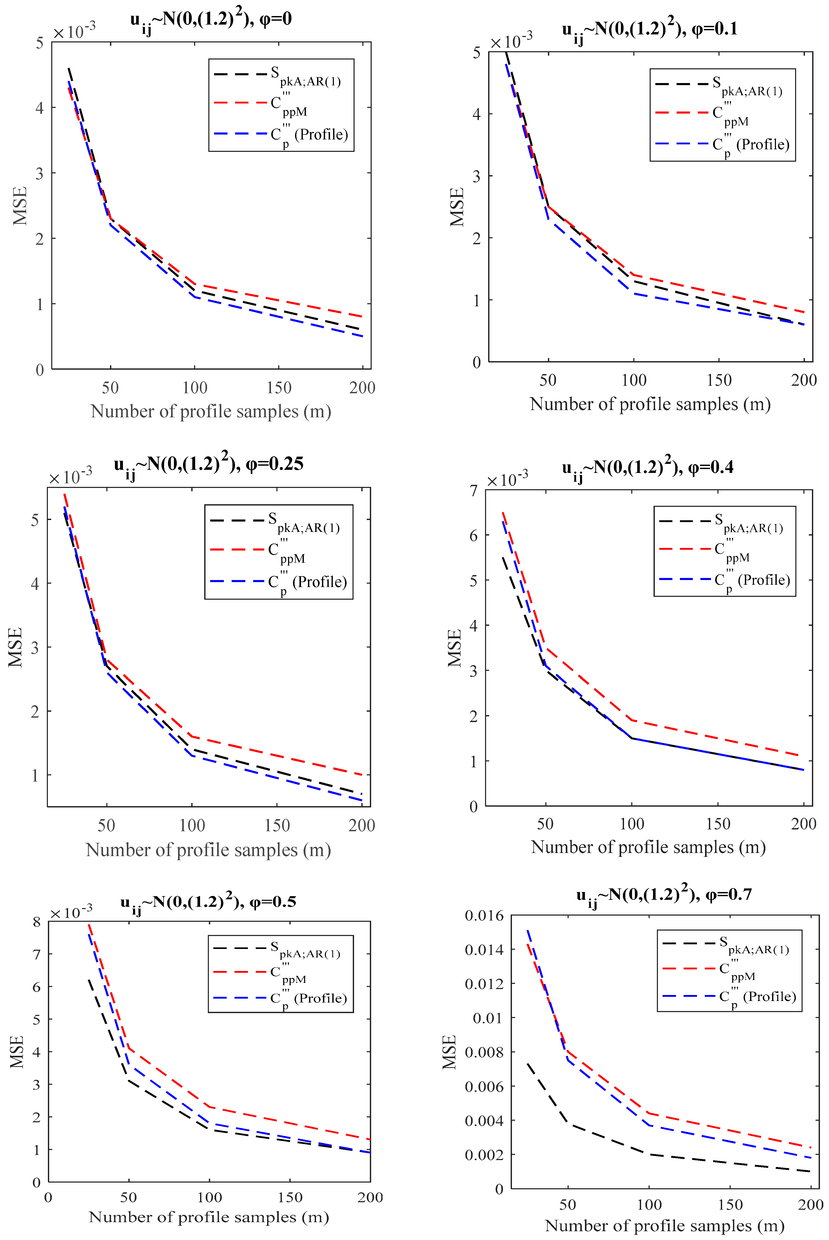
According to Table 2, Table 3 and Table 4, among the three PCIs ( S p k A ; A R ( 1 ) , C p p M , C p ( P r o f i l e ) ), the index C ^ p P r o f i l e , which significantly has the least bias, indicates that its mean is the most accurate representation of the true value. Additionally, regarding the MSE values, the index C ^ p P r o f i l e outperforms the index S ^ p k A ; A R ( 1 ) , especially for correlation coefficient φ less than 0.7. Also, the differences in MSE values of the indices C ^ p P r o f i l e and C p p M are negligible. The smallest bias and MSE values are highlighted in Table 2, Table 3 and Table 4. On the other hand, the number of profile samples m affects the estimates of all PCIs. As the number of profile samples m increases, the values of bias and MSE for all PCIs decrease. Figure 1, Figure 2 and Figure 3 clearly depict the findings about the performance evaluations of PCIs based on the MSE criterion for different correlation coefficients φ . Similar results can be drawn when the mean of the error terms is 0.1 under different variances. Results are available from the authors upon request. Hence, regarding bias and MSE, the suggested index C p P r o f i l e and the existing index S p k A ; A R ( 1 ) work best, respectively, for cases up to φ = 0.5 and φ > 0.5 .

4.2. Simulation Study for SLP in the Presence of WPAC

In this subsection, the following in-control SLP model in Equation (23) with within-profile autocorrelation ( ρ 0 ,   φ = 0 ) and ten fixed X i -values of 1, 2, 3, 4, 5, 6, 7, 8, 9, and 10 is considered similar to Wang and Tamirat [35]. The conditions in the simulated cases are the same as those in the Wang and Tamirat [35] simulation setting and include four profile samples ( m 25 ,   50 ,   100 ,   200 ), six correlation coefficients ( ρ 0 ,   0.1 ,   0.25 ,   0.4 ,   0.5 ,   0.7 ), and six error terms ( u i j ~ N ( 0 , 0.8 2 ) , u i j ~ N ( 0 , 1.0 2 ) , u i j ~ N ( 0 , 1.2 2 ) , u i j ~ N ( 0 , 0.8 2 ) , u i j ~ N ( 0 , 1.0 2 ) , u i j ~ N ( 0 , 1.2 2 ) ). The SLs and target values of the response variable at ten fixed X i -values are shown in Table 1.
For each simulated case, we calculated the index S ^ p k A ; A R ( 1 ) given by Equation (8) and description in Section 2.3.2, the index C ^ p P r o f i l e based on the method described in Section 3.2, and the index C ^ p p M using the same procedure as described in Section 3.2 for C p P r o f i l e . The simulations are repeated 10,000 times, and the average values of S ^ p k A ; A R ( 1 ) , C ^ p P r o f i l e , and C ^ p p M are obtained and reported. For each simulated case, the true values of PCIs are calculated using the actual model parameters and listed (for more information, see Appendix B). Moreover, the bias and MSE for the PCIs are calculated. Table 5, Table 6 and Table 7 and Figure 4, Figure 5 and Figure 6 illustrate the simulation findings.
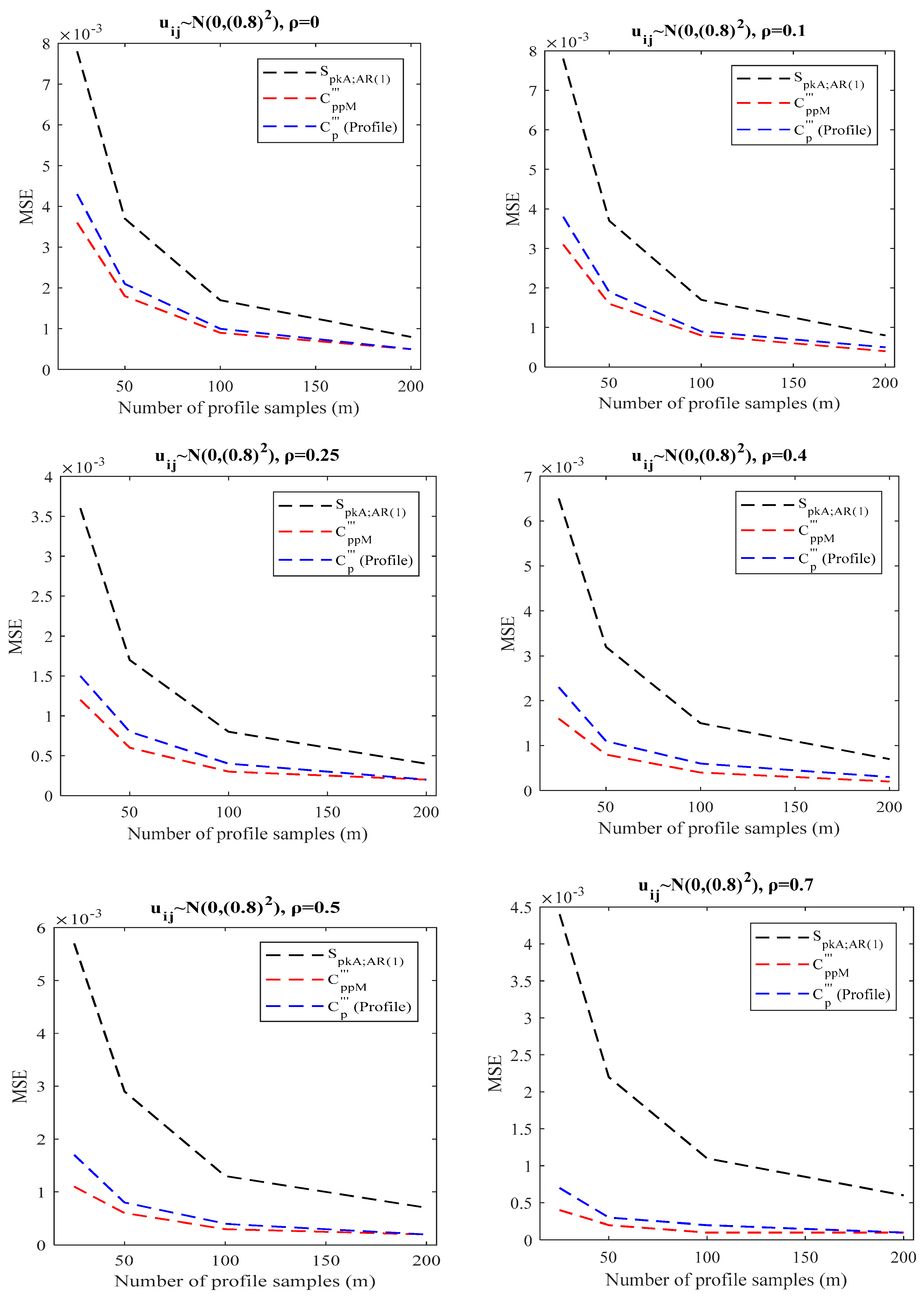
From Table 5, Table 6 and Table 7, it can be seen that the estimates of the index C p ( P r o f i l e ) have smaller bias and MSE values than S p k A ; A R ( 1 ) in all simulated cases. Of course, these values are also improved by increasing the number of profile samples. Additionally, Table 5, Table 6 and Table 7 demonstrate the superiority of the index C p ( P r o f i l e ) over C p p M in terms of smaller bias values. Furthermore, as can be seen in Figure 4, Figure 5 and Figure 6, the differences in MSE values of the indices C p ( P r o f i l e ) and C p p M are negligible, while the corresponding differences are significant for the indices C p ( P r o f i l e ) and S p k A ; A R ( 1 ) . The smallest bias and MSE values are highlighted in Table 5, Table 6 and Table 7. Similar results are obtained when the error terms follow u i j ~ N ( 0.1 , 0.8 2 ) , u i j ~ N ( 0.1 , 1.0 2 ) , and u i j ~ N ( 0.1 , 1.2 2 ) . As a result, simulation studies show that the recommended index C p ( P r o f i l e ) has superior performance compared to the other two PCIs.

4.3. Simulation Study for SLP in the Presence of BAC

To investigate the performance of the proposed method in evaluating the capability of SLP with BAC effects, the in-control SLP in Equation (23) with BAC effects and four fixed X i -values of 2, 4, 6, and 8 are considered. In this subsection, we consider the same simulated cases as before with the correlation coefficients ( ρ = φ 0 ,   0.1 ,   0.25 ,   0.4 ,   0.5 ,   0.7 ). The SLs and target values for the response variable at four fixed X i -values are shown in Table 1.
For each simulated case, we calculated the index C ^ p P r o f i l e based on the method described in Section 3.3. The simulations are repeated 10,000 times, and the average values of C ^ p P r o f i l e are obtained and reported. For each simulated case, the true values of C p P r o f i l e are calculated using the actual model parameters and listed (for more information, see Appendix C). Moreover, the bias and MSE associated with the index C ^ p P r o f i l e are calculated. The results of the simulation study are presented in Table 8.
From Table 8, it is concluded that the index C p P r o f i l e yields small bias and MSE values. The findings of the study reveal that the proposed method is quite efficient in evaluating the capability of SLP with BAC effects, and the performance of C p P r o f i l e keeps increasing with an increase in the number of profile samples as well as the correlation coefficients ρ and φ values.

4.4. Findings of the Simulation Studies

In this section, we discuss how to select a suitable PCI to conduct capability analysis considering the four possible SLPs in practical applications using bias and MSE criteria.
  • When there is no within and between profiles autocorrelation ( ρ = φ = 0 ), the index C p P r o f i l e that has superior performance than its competitors (see Table 2, Table 3, Table 4, Table 5, Table 6 and Table 7, when ρ = φ = 0 ) is suggested.
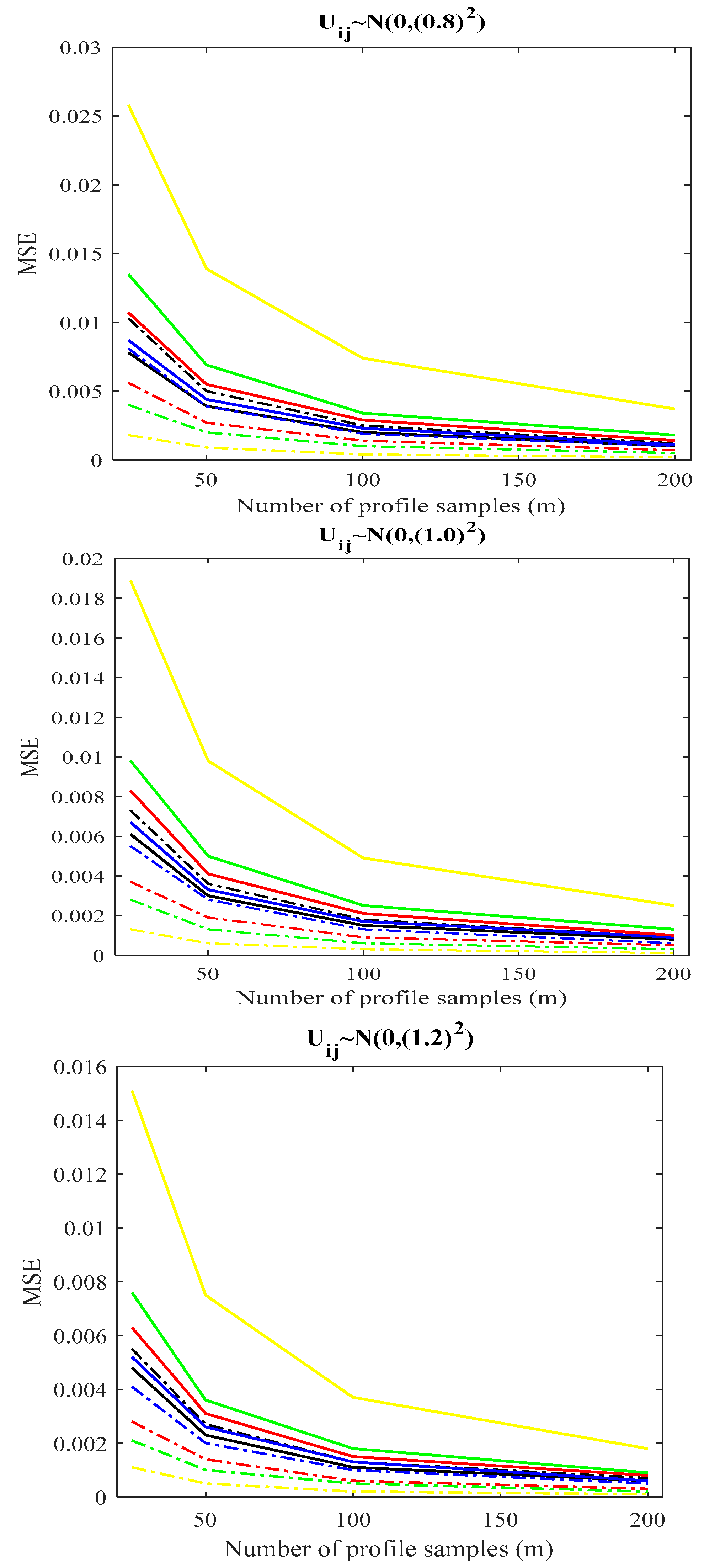
  • When there is a BPAC effect (( ρ = 0 ,   φ > 0 )), one can use the transformations in Section 3.1 and Section 3.3 as two options for recommending PCI. To select the superior transformation, a comparison between the proposed indices in Section 3.1 and Section 3.3 is provided. We conducted the same simulation studies in Section 4.1 ( ρ = 0 ,   φ = 0.1 ,   0.25 ,   0.4 ,   0.5 ,   0.7 ) and calculated the proposed index in Section 3.3. Table 9 displays the outcomes of the simulations. Based on the simulation results in the last columns of Table 2, Table 3, Table 4 and Table 9, as well as Figure 7, as φ increases, the difference between the two methods becomes more apparent, and the proposed index in Section 3.3 outperforms the proposed index in Section 3.1, especially for φ 0.25 with regard to bias and MSE criteria. Additionally, Figure 7 clearly shows these findings based on MSE criteria. Similarly, it can be observed that the suggested index in Section 3.3 generally has better bias and MSE than the index S p k A ; A R ( 1 ) in Section 2.3.1 by comparing the first column of Table 2, Table 3 and Table 4 with the findings of Table 9. Thus, when there is a BPAC effect, we suggest using the proposed index C p P r o f i l e discussed in Section 3.3.
  • When there is a WPAC effect ( ρ > 0 ,   φ = 0 ), the proposed index in Section 3.2 can be used because the transformation method in Equation (22) reduces to Equation (20), and according to simulation results in Section 4.2, the index C p P r o f i l e outperforms its competitors (see Table 5, Table 6 and Table 7 and Figure 4, Figure 5 and Figure 6).
  • When there is a BAC effect ( ρ > 0 ,   φ > 0 ), the proposed index C p P r o f i l e in Section 3.3 is recommended.

5. Bootstrap Confidence Intervals for C p ( P r o f i l e ) in the Presence of BAC

To enhance the reliability of the proposed index in Section 3.3, the nonparametric bootstrap method of Efron [44] is employed to determine confidence intervals for the proposed index as its underlying distribution is unknown. Both standard bootstrap (SB) and percentile bootstrap (PB) methods [45] will be used and evaluated in terms of relative coverage through a simulation study.
Let m profile samples from an in-control SLP process in the form ( X i , Y i j ) ; i = 1 , 2 , , n and j = 1 , 2 , , m with correlation coefficients ρ 0 ,   φ 0 be collected. A bootstrap sample is denoted by ( X i * , Y i j * ) ;   i = 1 , 2 , , n and j = 1 , 2 , , m is a sample extracted by substitution using the original sample. Suppose the resampling process is repeated B times. We use the B samples to obtain B bootstrap estimates of the index C p ( P r o f i l e ) based on the proposed method in Section 3.3. The B bootstrap estimates of C p ( P r o f i l e ) are denoted by C ^ p ( P r o f i l e ) k * , k = 1 , 2 , , B . These estimates are ordered from the smallest to the largest, denoted by C ^ p ( P r o f i l e ) ( 1 ) * , C ^ p ( P r o f i l e ) ( 2 ) * , , C ^ p ( P r o f i l e ) ( B ) * . Subsequent sections detail the construction of two types of bootstrap confidence intervals.

5.1. Standard Bootstrap (SB) Confidence Interval

Let C p ¯ ( P r o f i l e ) * and S * be the mean and standard deviation of C ^ p ( P r o f i l e ) k * , k = 1 , 2 , , B , given by
C ¯ p ( P r o f i l e ) * k = 1 B C ^ p ( P r o f i l e ) k * B ,
and
S * = k = 1 B C ^ p ( P r o f i l e ) k * C ^ p ( P r o f i l e ) * 2 B 1 .
Thus, 100 1 α % SB confidence interval for C p ( P r o f i l e ) can be obtained by
C ¯ p ( P r o f i l e ) * Z ( 1 α 2 ) S * , C ¯ p ( P r o f i l e ) * + Z ( 1 α 2 ) S * .
where Z ( 1 α 2 ) is the 100 1 α 2 % of the standard normal distribution.

5.2. Percentile Bootstrap (PB) Confidence Interval

According to ordered bootstrap estimates, C ^ p ( P r o f i l e ) ( k ) * ,   k = 1 , 2 , , B , the 100 1 α % PB confidence interval for C p ( P r o f i l e ) can be presented by
C ^ p ( P r o f i l e ) ( B . α 2 ) * , C ^ p ( P r o f i l e ) ( B . 1 α 2 ) * .

5.3. Simulation Study: Confidence Interval Evaluation

In this subsection, a series of simulations are carried out to assess the performance of the proposed confidence intervals for C p ( P r o f i l e ) in analyzing the capability of SLP with BAC. Using the same dataset as in Section 4.3, 10,000 simulation runs were performed for various error term and correlation coefficient combinations (see the first column of Table 10). For each simulation, 1000 bootstrap samples ( B = 1000 ) were generated based on a different number of profile samples m 25,50,100,200 , to construct 95% confidence intervals using both bootstrap methods. The performance of confidence intervals is evaluated by the relative coverage metric, which is the ratio of coverage percentage to the average length of the confidence interval. In Table 10, the average of estimated C p ( P r o f i l e ) over 10,000 runs as well as the average confidence interval ( C I ¯ ) and relative coverage of C p ( P r o f i l e ) are reported. For better clarification, Pseudocode 2 represents the procedure for computing confidence intervals for C p ( P r o f i l e ) in the presence of BAC. The green lines are some comments about the codes.
Pseudocode 2. The procedure for computing the bootstrap confidence interval for  C ^ p ( P r o f i l e ) ,   C I ¯  and relative coverage using Monte Carlo simulation
Consider the in-control profile model, SLs’ function, sigma = 1, n , m , ρ , and φ .
errorpre = normrnd (0,sigma, [1,n]); % Normal preerror with size n
while (we do not reach the number of generated samples)
     aij = normrnd (0,sigma,[1,n]);                   % Normal variable with size n
      % Generate data
     for i = 1:n
           if (i == 1)
                 epsilon(i) = φ × errorpre(i) + aij(i);
           else
                 epsilon(i) = ρ × epsilon (i−1) + φ × errorpre(i) − φ × ρ × errorpre (i−1) + aij(i);
           endif
      endfor
      Y = A 0 + A 1 X + epsilon;  % Equation (1)
      errorpre = epsilon;   % Update the previous error
endwhile
% It is necessary to transfer the SLs as we apply the transformation of the in-control profile model.% The details for computations were given in Section 3.3.
Apply the transformation on the SLs.
Compute C p ( P r o f i l e ) based on Equation (10) and the in-control parameters.
for rep = 1:1:10,000
   Generate m profiles by the in-control model.
   do a bootstrap loop 1000 times
     Generate a bootstrap with resampling profiles based on the m generated profile.
      % The parameter estimation is performed based on the computations given in Section 3.3.
      ( a 0 , a 1 , σ ^ 2 ) = Estimate the profile parameters, including intercept, slope, and standard deviation, based on the m profiles.
     Compute μ ^ Y X = a 0 + a 1 X   and   σ ^ 2   based on the proposed method for SLP with BAC.
      C ^ p ( P r o f i l e ) k * = Estimate C ^ p ( P r o f i l e ) k * based on the Equation (10) by μ ^ Y and σ ^ 2 k = 1 , 2 , , B .
     Store the values C ^ p ( P r o f i l e ) k * .
     Sort C ^ p ( P r o f i l e ) k * , k = 1 , 2 , , B from the smallest to largest.
      endloop
    C ^ p ( P r o f i l e ) r e p = k = 1 1000 C ^ p ( P r o f i l e ) k * 1000 .
   Compute the SB and PB confidence intervals.
   Record the length of intervals.
endfor
Compute the average of 10,000 C ^ p ( P r o f i l e ) r e p values.
Compute the average of confidence intervals ( C I ¯ ).
Compute the average interval length, coverage percentage, and relative coverage for the SB and PB approaches.
Table 10 presents the relative coverage values for the confidence intervals of the index C p ( P r o f i l e ) for SLP with BAC based on the SB and PB methods under various simulation cases. The results consistently demonstrate that the SB method outperforms the PB method in terms of related coverage in almost all cases, indicating higher coverage percentages with shorter interval lengths. The higher values of relative coverage are highlighted in Table 10. Furthermore, a larger number of profile samples m and higher correlation coefficients improve relative coverage for both methods. While the SB method generally exhibits superior performance, it is essential to note that the relative performance of the two methods might vary under different conditions. Future research could explore the sensitivity of the SB and PB methods to different autocorrelation structures, sample sizes, and process characteristics.

6. Illustrative Example

To bridge the gap between simulation and real-world applications, a general framework in the following steps to a proper implantation in real-world scenarios in different fields, such as manufacturing, metrology, and environmental monitoring, is provided.
  • Data Collection: Real-world data should be collected in accordance with appropriate sampling plans to ensure representativeness and statistical power.
  • Data Preprocessing: Data cleaning and preprocessing steps are essential to address issues such as missing values, outliers, and trends.
  • Parameter Estimation: The parameters of the autocorrelation models can be estimated using standard statistical methods, such as maximum likelihood or least squares.
  • Phase I Profile Monitoring: The process stability should be assessed and the in-control profile parameters estimated.
  • Process Capability Assessment: The proposed process capability index can be calculated based on the estimated parameters and the observed data.
  • Interpretation: The results should be interpreted in the context of the specific application and used to inform decision making.
To streamline the illustrative example, this paper concentrates solely on the final steps of the proposed methodology. Consequently, the processes of data collection, preprocessing, and parameter estimation are excluded from the current analysis. Instead, the primary focus is on the evaluation of process capability through the proposed index and the subsequent interpretation of results within the specific application context. Hence, we considered a calibration system used in the chemical industry to illustrate the use of the proposed methodology and verify its applicability in real-life situations. The chemical experimental instruments usually consist of gas sensors to detect toxic and unnatural processes. They are usually kept away from the laboratory to ensure accurate measurements and prevent potential safety hazards. When moving these devices to a new sensing environment, some challenges arise in the new conditions, such as (i) the fact that the calibration parameters may need to be adjusted or recalibrated to ensure accurate readings. (ii) Gas sensors can exhibit cross-sensitivity, meaning they may respond not only to the target gas but also to other gases present in the environment. (iii) Different sensing environments may present varying temperatures, humidity levels, and atmospheric pressures. These conditions can impact the performance and reliability of gas sensors. (iv) Moving gas sensing devices to a new environment involves proper physical installation. Factors such as location, mounting, and accessibility need to be considered to ensure representative and effective gas detection. To handle this situation, a profile model can be applied to address calibration issues and ascertain their proper performance over time. The calibration of metal oxide (MOX) as a gas sensor has been discussed and monitored in other related studies [18,46,47]. According to these studies, a functional relationship is considered between the resistance (R) of the sensor as the response variable and the concentrations of carbon monoxide as the explanatory variable. Four fixed levels of carbon monoxide (CO) concentration as 25, 100, 125, and 150 ppm are considered. Based on 3287 in-control SLPs, the calculated reference profile is Y i j = 71.741 + 0.0176 X i + ε i j , where ε i j ~ N ( 0,0.142 ) . Nadi et al. [18] investigated the effect of adding additive material to increase the efficiency of the process. Although it can be useful for this purpose, some changes in the reference relationship may occur in such a way that the new formula is obtained between the resistance and carbon concentration, as given by
Y i j = 71.741 + 0.0176 X i + ε i j , ε i j = 0.289 ε i 1 j + a i j , a i j = 0.565 ε i j 1 + u i j , u i j ~ N 0 , 0.0742 , i = 1 , 2 , 3 , 4 . j = 1 , 2 , .
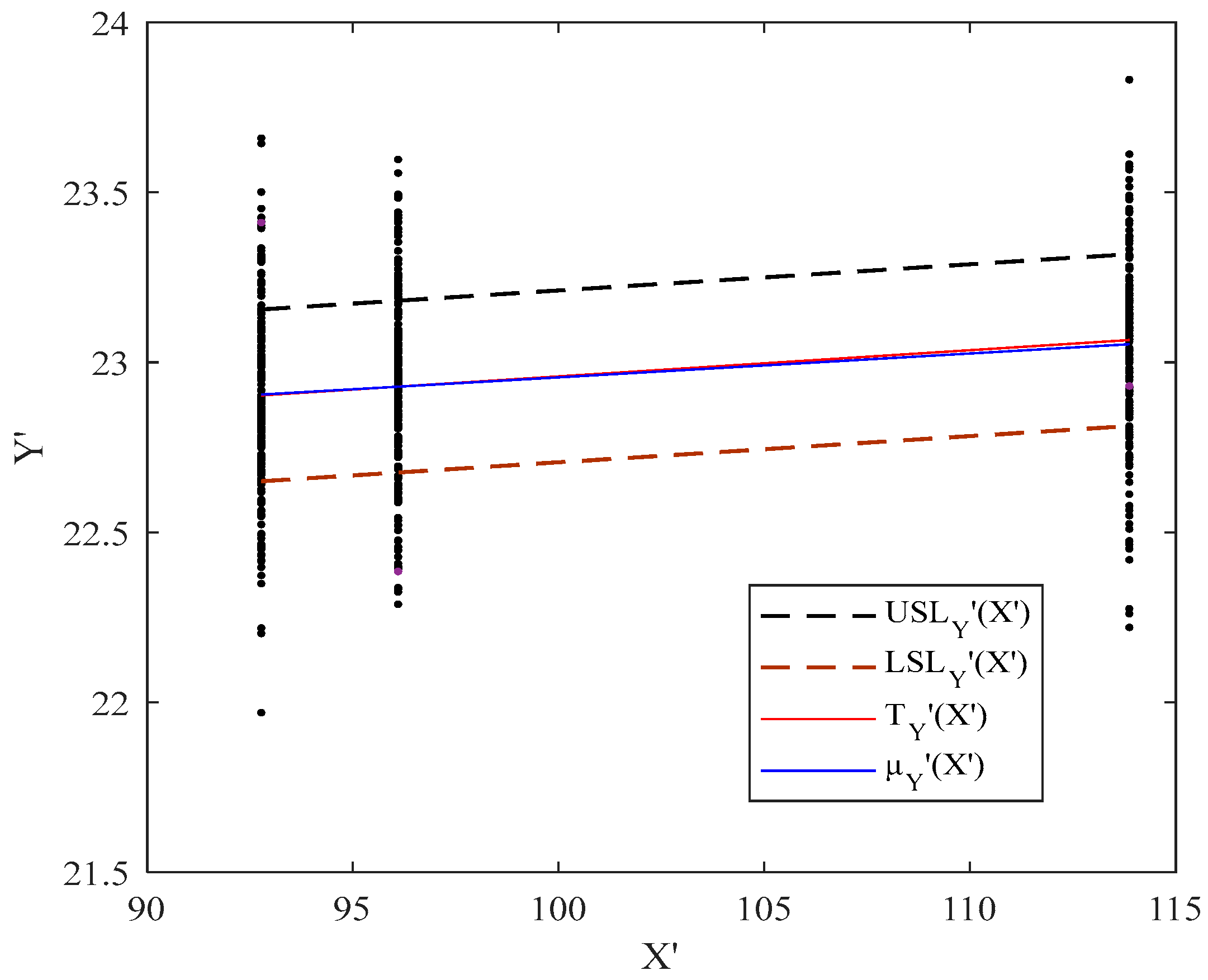
To illustrate how to measure the calibration of MOX capability, we generate datasets of 200 profiles based on the in-control model in Equation (28). Since the SLs for this process do not exist, we set the SLs for the resistance (R) of the MOX at different concentrations of carbon monoxide based on the natural tolerance limits of the process. Therefore, the functional SLs and target value are calculated as L S L Y X = 70.9238 + 0.0176 X , U S L Y X = 72.5582 + 0.0176 X , and T Y X = 71.7410 + 0.0176 X , respectively, where X 25 , 150 . The methods proposed in Section 3 can be used to assess process capability for the calibration process. According to Equation (22), L S L Y X = 21.9357 + 0.0077 X , U S L Y X = 22.4412 + 0.0077 X , and T Y X = 22.1844 + 0.0077 X , and μ Y X = 22.2558 + 0.0070 X are obtained, where X 92.7750,113.8750 , and σ ^ 2 = 0.0774 . These transformed functional limits for the calibration of MOX data are depicted in Figure 8.
The estimated value for the index C p P r o f i l e is 0.3001, with the following 95% confidence intervals:
S B : 0.2867 , 0.3265 ,   P B : 0.2872 , 0.3270
According to Figure 8, it is shown that although the process mean almost coincides with the target line, the process variation is undesirable. Since the value of the capability index is less than 1 with 95% confidence intervals, we conclude that the calibration process is incapable. Therefore, corrective actions to reduce process variance are required.

7. Conclusions and Future Works

In this article, we studied the capability analysis of SLP with different possible autocorrelation effects in real applications. The SLP with a general error model, which is adaptable enough to model four possibilities for the SLP in practical applications, was taken into consideration. The new functional capability index C p ( P r o f i l e ) for the SLP in the absence of autocorrelation effects was introduced. In order to evaluate the capability of the SLP with BPAC, WPAC, and BAC, where autocorrelation structures follow an AR(1) model, three distinct approaches were presented. The basic idea was first applying the transformation to eliminate BPAC, WPAC, and/or BAC, and then estimating PCIs for SLP using independent statistics. The simulation studies in the presence of each of the two autocorrelation effects (BPAC and WPAC) were conducted to investigate and compare the performance of the proposed PCIs with those of the existing ones proposed by Wang and Tamirat [34] and Wang and Tamirat [35] in terms of bias and MSE criteria. Moreover, we compared these PCIs with another existing PCI for SLP (index C p p M ) to draw conclusions about the proposed method. In brief, the results of the simulation study showed that:
  • In the case of BPAC, the new index C p P r o f i l e had a bias that was noticeably lower than the bias of the indices S p k A ; A R 1 and C p p M for all the values of correlation coefficients φ , and its MSE was also lower than the MSE of S p k A ; A R 1 especially for φ < 0.7 , and approximately equal to that of C p p M .
  • In the case of WPAC, the new index C p P r o f i l e outperformed the index S p k A ; A R 1 due to its smaller bias and MSE in all simulated cases. In addition, the index C p P r o f i l e performed better than C p p M due to its close MSE to the index C p p M and extremely small bias.
  • In two cases, BPAC and WPAC, all PCIs performed well with a larger sample size.
The results of the simulation study showed that the recommended index C p ( P r o f i l e ) had superior performance over its competitors. Additionally, the effectiveness of the suggested index for SLP with BAC was examined in various simulation instances; bootstrap confidence intervals were obtained using the two methods SB and PB, and their performance was assessed using simulation studies. The results indicated that the new index can accurately reflect the actual performance of SLP with BAC. Additionally, when only the BPAC effect was present, the proposed index for SLP with BAC performed better than the proposed index for SLP with the BPAC effect, particularly for φ 0.25 . Additionally, the SB method bootstrap confidence intervals performed better than the PB method for almost all simulated cases in terms of the relative coverage metric. Finally, an illustrative example in a calibration system from the chemical industry demonstrated the usefulness of the proposed PCI for SLP with BAC in practice.
Future studies may include analyzing the proposed methods in the case of random explanatory variable X or when the assumption of normality of error terms in the SLP model is violated. In addition, introducing robust PCIs for SLP as well as other types of profiles like multivariate profiles, multiple linear profiles, and logistic regression profiles in the presence of both within- and between-profile autocorrelations can be considered as future works. Analyzing the proposed methods in the case of within- and between-profile autocorrelation with other autocorrelation patterns, such as autoregressive moving average (ARMA) and vector ARMA (VARMA), also requires further study.

Author Contributions

All authors contributed to the study’s conception and design. All authors have read and agreed to the published version of the manuscript.

Funding

The authors declare that no funds, grants, or other support were received during the preparation of this manuscript.

Data Availability Statement

The source code and data used to produce the results and analyses presented in this manuscript are available and will be sent, if peer reviewers will be asked to assess.

Conflicts of Interest

The authors declare that they have no conflicts of interest.

Appendix A

Calculating the true values of  S p k A ; A R ( 1 ) , C p p M , and C p ( P r o f i l e ) for SLP with BPAC when u i j ~ N ( 0 , 0.8 2 ) , φ = 0.1 , X i 2 , 4 , 6 , 8 , L S L i 2.5 , 6.85 , 11.25 , 16.25 , U S L i 10,14.35 , 18.75 , 23.75 , T i 6.25 , 10.60 , 15 , 20 .
  • Calculating the true values of  S p k A ; A R ( 1 ) : By considering L S L i , U S L i , T i , μ i = 3 + 2 X i , and σ 2 = σ 2 1 φ 2 = 0.8 2 1 0.1 2 = 0.6465 , Equation (6) is used to first determine the values of S p k i for 4 levels of the explanatory variable, which are calculated as 1.3008, 1.4401, 1.5547, and 1.2015, respectively. The values of P i are then calculated using Equation (7) and are equal to 0.9999, 1, 1, and 0.9997. Therefore, P = i = 1 4 P i 4 value is calculated, which is equal to 0.9999. Using Equation (8), the index S p k A ; A R ( 1 ) is finally calculated to be 1.2916.
  • Calculating the true value of   C p p M : By considering L S L i , U S L i , T i , μ i = 3 + 2 X i , and σ 2 = 0.8 2 , we must first calculate the values of C p p i for each of the 4 levels of the explanatory variable using Equation (4). These values are 1.0943, 1.3816, 1.5625, and 0.9067, respectively. Finally, the C p p M = i = 1 4 C p p i 4 is calculated to be 1.2363.
  • Calculating the true value of   C p ( P r o f i l e ) : By considering L S L i , U S L i , T i , μ Y ( X ) = 3 + 2 X , and σ 2 = 0.8 2 , firstly, the regression lines are fitted to the values of L S L i , U S L i , and T i , to yield the functional SLs and target line as L S L Y X = 2.2 + 2.2825 X , U S L Y X = 5.3 + 2.2825 X , and T Y X = 1.55 + 2.2825 X , where X 2,8 . Then, to calculate C p ( P r o f i l e ) , the location of μ Y ( X ) relative to T Y ( X ) is determined based on the method proposed in Pakzad and Basiri [39]. Figure A1 shows that μ Y ( X ) and T Y ( X ) cross at x m = 5.1327 and C p ( P r o f i l e ) is calculated as 1.3160 using Equation (16).
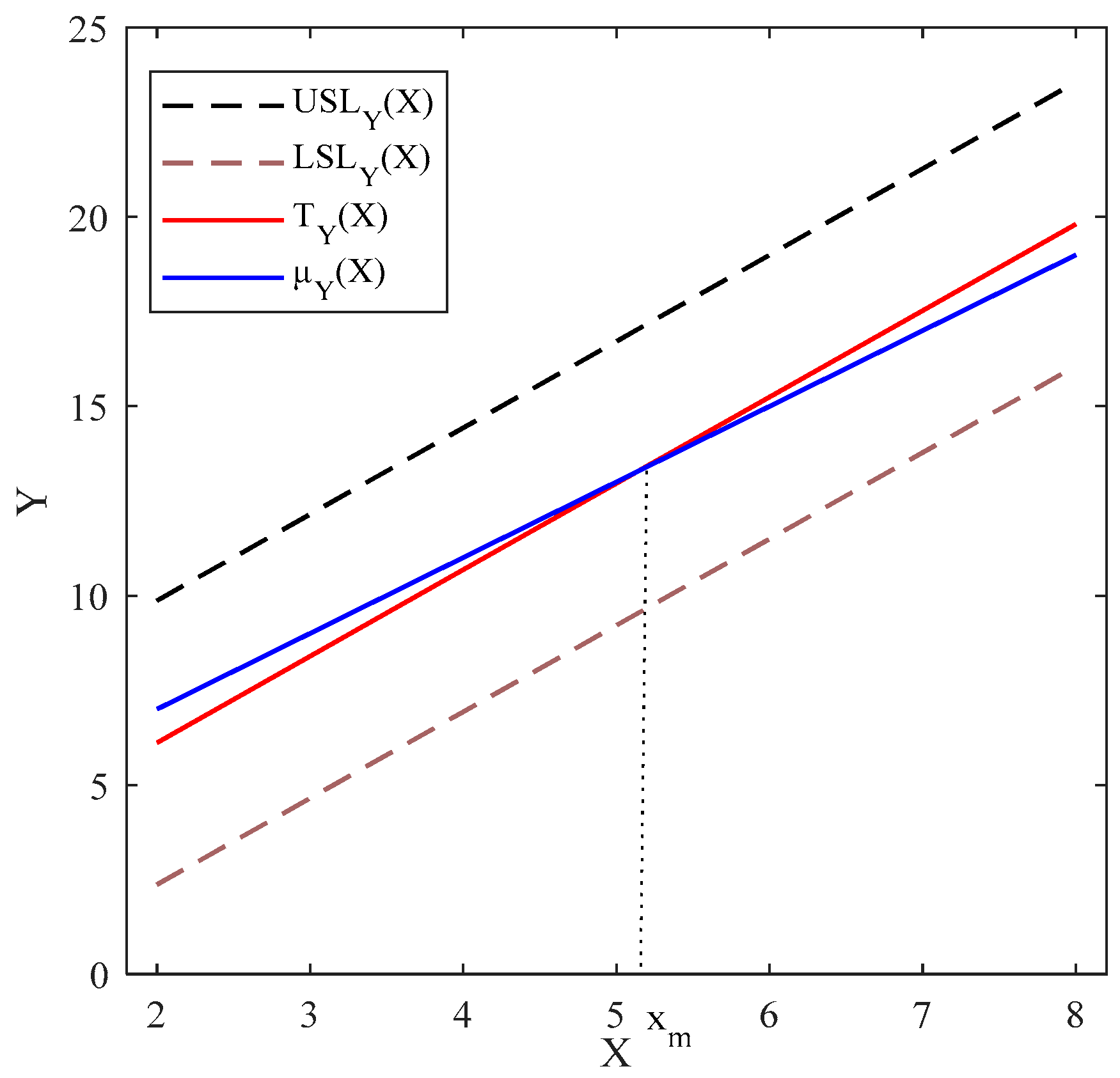
Figure A1. The location of μ Y ( X ) relative to T Y ( X ) for SLP with BPAC.
Mathematics 12 02549 g0a1

Appendix B

Calculating the true values of S p k A ; A R ( 1 ) , C p p M , and C p ( P r o f i l e ) for SLP with WPAC when u i j ~ N ( 0 , 0.8 2 ) , ρ = 0.1 , X i 1 , 2 , , 10 , L S L i , U S L i , T i where results are shown in Table 1.
  • Calculating the true values of  S p k A ; A R ( 1 ) : By considering L S L i , U S L i , T i , μ i = 3 + 2 X i , and σ 2 = σ 2 1 ρ 2 = 0.8 2 1 0.1 2 = 0.6465 , first Equation (6) is used to calculate the values of S p k i for 10 levels of the explanatory variable as 1.1344, 1.3008, 1.3566, 1.4401, 1.5517, 1.5547, 1.3964, 1.2015, 1.1738, and 1.4975, respectively. The values of P i are then calculated using Equation (7) as 0.9993, 0.9999, 1, 1, 1, 1, 1, 0.9997, 0.9996, and 1. P = i = 1 10 P i 10 is thus calculated to be 0.9998. Using Equation (8), the index S p k A ; A R ( 1 ) is finally calculated to be 1.2579.
  • Calculating the true value of   C p p M : By considering L S L i , U S L i , T i , μ i = 3 + 2 X i , and σ 2 = 0.8 2 , first the transformation method of Soleimani et al. [13] is applied. Therefore, we have X i 1.9 , 2.8 , 3.7 , 4.6 , 5.5 , 6.4 , 7.3 , 8.2 , 9,1 , L S L i 2.492 , 4.39 , 6.386 , 8.515 , 10.33 , 12.635 , 14.874 , 16.695 , 17.668 , U S L i 9.242 , 11.14 , 13.136 , 15.265 , 17.08 , 19.385 , 21.624 , 23.445 , 24.418 , T i 5.867 , 7.765 , 9.761 , 11.89 , 13.705 , 16.01 , 18.249 , 20.07 , 21.043 , and μ i = 2.7 + 2 X i . The values of C p p i for 9 levels of X i are then determined using Equation (4) as 1.0640, 1.1396, 1.2817, 1.4061, 1.4064, 1.1587, 0.8347, 0.8208, and 1.3818, respectively. The C p p M = i = 1 9 C p p i 9 is finally calculated as 1.1660.
  • Calculating the true value of  C p ( P r o f i l e ) : By considering L S L i , U S L i , T i , μ Y ( X ) = 3 + 2 X , and σ 2 = 0.8 2 , as well as using the transformation method proposed by Soleimani et al. [13], we obtain X i , L S L i , U S L i , T i , and μ Y X = 2.7 + 2 X . Then, the regression lines are fitted to the values of L S L i , U S L i , and T i , to obtain the functional transformed SLs and target line as L S L Y X = 1.6486 + 2.1984 X , U S L Y X = 5.1014 + 2.1984 X , and T Y X = 1.7264 + 2.1984 X , where X 6.5,20.9 . Finally, to calculate C p ( P r o f i l e ) , the location of μ Y X relative to T Y X is determined based on the method proposed in Pakzad and Basiri [39]. As we can see in Figure A2, μ Y X and T Y X , intersect at x m = 4.9064 and C p ( P r o f i l e ) derived as 1.2238 based on Equation (16).
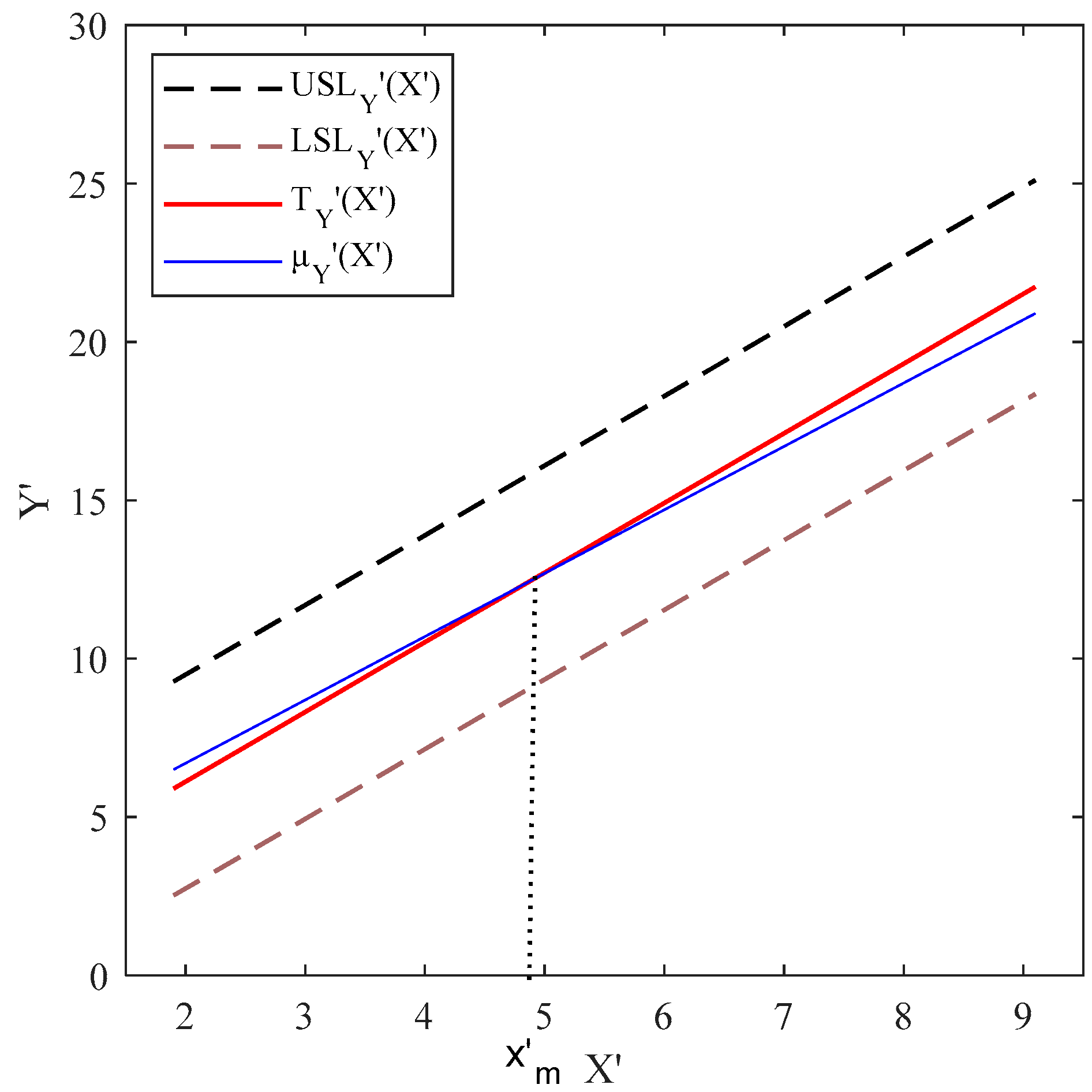
Figure A2. The location of μ Y ( X ) relative to T Y ( X ) for SLP with WPAC.
Mathematics 12 02549 g0a2

Appendix C

Calculating the true value of C p ( P r o f i l e ) for SLP with BAC when u i j ~ N ( 0 , 0.8 2 ) , ρ = φ = 0.1 , X i 2 , 4 , 6 , 8 , L S L i 2.5 , 6.85 , 11.25 , 16.25 , U S L i 10,14.35 , 18.75 , 23.75 , T i 6.25 , 10.60 , 15 , 20 .
  • Calculating the true value of  C p ( P r o f i l e ) : By considering L S L i , U S L i , T i , μ Y ( X ) = 3 + 2 X , and σ 2 = 0.8 2 , the regression lines are first fitted to the values of L S L i , U S L i , and T i , resulting in the functional SLs and target line as L S L Y X = 1.7820 + 2.0543 X , U S L Y X = 4.2930 + 2.0543 X , and T Y X = 1.2555 + 2.0543 X , where X 2,8 . Then the transformation by Soleimani et al. [13] is used. According to Equation (22), L S L Y X = 1.6486 + 2.1984 X , U S L Y X = 5.1014 + 2.1984 X , and T Y X = 1.7264 + 2.1984 X , and μ Y X = 2.43 + 1.8 X , where X 3.8,7.4 . Then, to calculate C p ( P r o f i l e ) , the location of μ Y X relative to T Y X is determined based on the method proposed in Pakzad and Basiri [39]. Figure A3 demonstrates that μ Y X and T Y X intersect at x m = 4.6195 and C p ( P r o f i l e ) obtained as 1.1387 based on Equation (16).
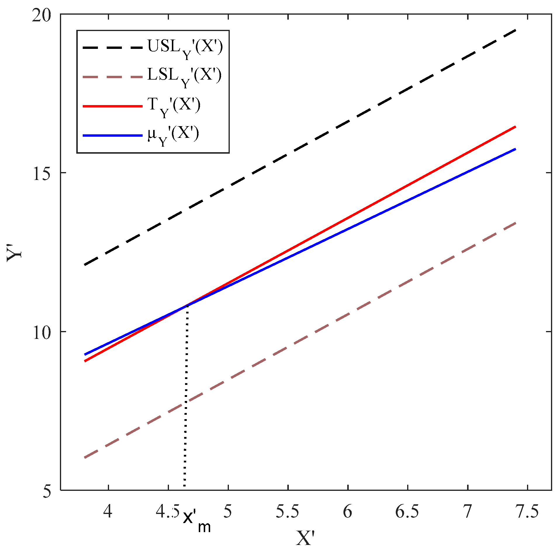
Figure A3. The location of μ Y ( X ) relative to T Y ( X ) for SLP with BAC.
Mathematics 12 02549 g0a3

References

  1. Gupta, S.; Montgomery, D.C.; Woodall, W.H. Performance evaluation of two methods for online monitoring of linear calibration profiles. Int. J. Prod. Res. 2006, 44, 1927–1942. [Google Scholar] [CrossRef]
  2. Kang, L.; Albin, S.L. On-Line Monitoring When the Process Yields a Linear Profile. J. Qual. Technol. 2000, 32, 418–426. [Google Scholar] [CrossRef]
  3. Kim, K.; Mahmoud, M.A.; Woodall, W.H. On the Monitoring of Linear Profiles. J. Qual. Technol. 2003, 35, 317–328. [Google Scholar] [CrossRef]
  4. Li, Z.; Wang, Z. An exponentially weighted moving average scheme with variable sampling intervals for monitoring linear profiles. Comput. Ind. Eng. 2010, 59, 630–637. [Google Scholar] [CrossRef]
  5. Xu, L.; Wang, S.; Peng, Y.; Morgan, J.P.; Reynolds, M.R.; Woodall, W.H. The Monitoring of Linear Profiles with a GLR Control Chart. J. Qual. Technol. 2012, 44, 348–362. [Google Scholar] [CrossRef]
  6. Chen, S.; Yu, J.; Wang, S. Monitoring of complex profiles based on deep stacked denoising autoencoders. Comput. Ind. Eng. 2020, 143, 106402. [Google Scholar] [CrossRef]
  7. Nassar, S.H.; Abdel-Salam, A.-S.G. Robust profile monitoring for phase II analysis via residuals. Qual. Reliab. Eng. Int. 2022, 38, 432–446. [Google Scholar] [CrossRef]
  8. Maleki, M.R.; Amiri, A.; Castagliola, P. An overview on recent profile monitoring papers (2008–2018) based on conceptual classification scheme. Comput. Ind. Eng. 2018, 126, 705–728. [Google Scholar] [CrossRef]
  9. Noorossana, R.; Amiri, A.; Soleimani, P. On the Monitoring of Autocorrelated Linear Profiles. Commun. Stat. Theory Methods 2008, 37, 425–442. [Google Scholar] [CrossRef]
  10. Wang, Y.-H.T.; Huang, W.-H. Phase II monitoring and diagnosis of autocorrelated simple linear profiles. Comput. Ind. Eng. 2017, 112, 57–70. [Google Scholar] [CrossRef]
  11. Khedmati, M.; Niaki, S.T.A. Phase II monitoring of general linear profiles in the presence of between-profile autocorrelation. Qual. Reliab. Eng. Int. 2016, 32, 443–452. [Google Scholar] [CrossRef]
  12. Wang, Y.-H.T.; Lai, Y. Monitoring of autocorrelated general linear profiles. J. Stat. Comput. Simul. 2019, 89, 519–535. [Google Scholar] [CrossRef]
  13. Soleimani, P.; Noorossana, R.; Amiri, A. Simple linear profiles monitoring in the presence of within profile autocorrelation. Comput. Ind. Eng. 2009, 57, 1015–1021. [Google Scholar] [CrossRef]
  14. Jensen, W.A.; Birch, J.B.; Woodall, W.H. Monitoring Correlation Within Linear Profiles Using Mixed Models. J. Qual. Technol. 2008, 40, 167–183. [Google Scholar] [CrossRef]
  15. Zhang, W.; Niu, Z.; He, Z.; He, S. Online monitoring of profiles via function-on-scalar model with an application to industrial busbar. Qual. Reliab. Eng. Int. 2022, 38, 3816–3828. [Google Scholar] [CrossRef]
  16. Niaki, S.T.A.; Khedmati, M.; Soleymanian, M.E. Statistical Monitoring of Autocorrelated Simple Linear Profiles Based on Principal Components Analysis. Commun. Stat. Theory Methods 2015, 44, 4454–4475. [Google Scholar] [CrossRef]
  17. Yeganeh, A.; Johannssen, A.; Chukhrova, N.; Abbasi, S.A.; Pourpanah, F. Employing machine learning techniques in monitoring autocorrelated profiles. Neural Comput. Appl. 2023, 35, 16321–16340. [Google Scholar] [CrossRef]
  18. Nadi, A.A.; Yeganeh, A.; Shadman, A. Monitoring simple linear profiles in the presence of within-and between-profile autocorrelation. Qual. Reliab. Eng. Int. 2023, 39, 752–775. [Google Scholar] [CrossRef]
  19. Alevizakos, V. Process Capability and Performance Indices for Discrete Data. Mathematics 2023, 11, 3457. [Google Scholar] [CrossRef]
  20. Perakis, M.; Xekalaki, E. On the relationship between process capability indices and the proportion of conformance. Qual. Technol. Quant. Manag. 2016, 13, 207–220. [Google Scholar] [CrossRef]
  21. Afshari, R.; Nadi, A.A.; Johannssen, A.; Chukhrova, N.; Tran, K.P. The effects of measurement errors on estimating and assessing the multivariate process capability with imprecise characteristic. Comput. Ind. Eng. 2022, 172, 108563. [Google Scholar] [CrossRef]
  22. Wang, S.; Chiang, J.-Y.; Tsai, T.-R.; Qin, Y. Robust process capability indices and statistical inference based on model selection. Comput. Ind. Eng. 2021, 156. [Google Scholar] [CrossRef]
  23. Alevizakos, V.; Koukouvinos, C. Evaluation of process capability in gamma regression profiles. Commun. Stat. Simul. Comput. 2022, 51, 5174–5189. [Google Scholar] [CrossRef]
  24. Guevara G, R.D.; Alejandra Lopez, T. Process capability vector for multivariate nonlinear profiles. J. Stat. Comput. Simul. 2022, 92, 1292–1321. [Google Scholar] [CrossRef]
  25. Wang, F.K.; Guo, Y.C. Measuring process yield for nonlinear profiles. Qual. Reliab. Eng. Int. 2014, 30, 1333–1339. [Google Scholar] [CrossRef]
  26. Bera, K.; Anis, M.Z. Process incapability index for autocorrelated data in the presence of measurement errors. Commun. Stat. Theory Methods 2023, 53, 5439–5459. [Google Scholar] [CrossRef]
  27. Cohen, A.; Amin, R. The effects of normal mixtures and autocorrelation on the fraction non-conforming. Commun. Stat. Simul. Comput. 2017, 46, 8105–8117. [Google Scholar] [CrossRef]
  28. Lundkvist, P.; Vannman, K.; Kulahci, M. A comparison of decision method for Cpk when data are autocorrelated. Qual. Control. Appl. Stat. 2013, 58, 451–452. [Google Scholar]
  29. Hosseinifard, S.Z.; Abbasi, B. Evaluation of process capability indices of linear profiles. Int. J. Qual. Reliab. Manag. 2012, 29, 162–176. [Google Scholar] [CrossRef]
  30. Hosseinifard, S.Z.; Abbasi, B. Process Capability Analysis in Non Normal Linear Regression Profiles. Commun. Stat. Simul. Comput. 2012, 41, 1761–1784. [Google Scholar] [CrossRef]
  31. Ebadi, M.; Shahriari, H. A process capability index for simple linear profile. Int. J. Adv. Manuf. Technol. 2013, 64, 857–865. [Google Scholar] [CrossRef]
  32. Wang, F.-K. A Process Yield for Simple Linear Profiles. Qual. Eng. 2014, 26, 311–318. [Google Scholar] [CrossRef]
  33. Wang, F. Measuring the Process Yield for Simple Linear Profiles with one-Sided Specification. Qual. Reliab. Eng. Int. 2014, 30, 1145–1151. [Google Scholar] [CrossRef]
  34. Wang, F.-K.; Tamirat, Y. Process yield analysis for autocorrelation between linear profiles. Comput. Ind. Eng. 2014, 71, 50–56. [Google Scholar] [CrossRef]
  35. Wang, F.; Tamirat, Y. Process Yield Analysis for Linear Within-Profile Autocorrelation. Qual. Reliab. Eng. Int. 2015, 31, 1053–1061. [Google Scholar] [CrossRef]
  36. Mehri, S.; Ahmadi, M.M.; Shahriari, H.; Aghaie, A. Robust process capability indices for multiple linear profiles. Qual. Reliab. Eng. Int. 2021, 37, 3568–3579. [Google Scholar] [CrossRef]
  37. Ganji, Z.A.; Gildeh, B.S. A new process capability index for simple linear profile. Commun. Stat. Theory Methods 2023, 52, 3879–3894. [Google Scholar] [CrossRef]
  38. Pakzad, A.; Razavi, H.; Gildeh, B.S. Developing loss-based functional process capability indices for simple linear profile. J. Stat. Comput. Simul. 2022, 92, 115–144. [Google Scholar] [CrossRef]
  39. Pakzad, A.; Basiri, E. A new incapability index for simple linear profile with asymmetric tolerances. Qual. Eng. 2023, 35, 324–340. [Google Scholar] [CrossRef]
  40. Ganji, Z.A.; Gildeh, B.S. A class of process capability indices for asymmetric tolerances. Qual. Eng. 2016, 28, 441–454. [Google Scholar] [CrossRef]
  41. Boyles, R.A. Brocess capability with asymmetric tolerances. Commun. Stat. Simul. Comput. 1994, 23, 615–635. [Google Scholar] [CrossRef]
  42. Bothe, D.R. Measuring Process Capability: Techniques and Calculations for Quality and Manufacturing Engineers; McGraw-Hill Companies: New York, NY, USA, 1997. [Google Scholar]
  43. Keshteli, R.N.; Kazemzadeh, R.B.; Amiri, A.; Noorossana, R. Developing functional process capability indices for simple linear profile. Sci. Iran. 2014, 21, 1096–1104. [Google Scholar]
  44. Efron, B. The Jackknife, the Bootstrap and other Resampling Plans; SIAM: Philadelphia, PA, USA, 1982. [Google Scholar]
  45. Efron, B.; Tibshirani, R. Bootstrap Methods for Standard Errors, Confidence Intervals, and Other Measures of Statistical Accuracy. Stat. Sci. 1986, 1, 54–75. [Google Scholar] [CrossRef]
  46. Abbas, T.; Mahmood, T.; Riaz, M.; Abid, M. Improved linear profiling methods under classical and Bayesian setups: An application to chemical gas sensors. Chemom. Intell. Lab. Syst. 2020, 196, 103908. [Google Scholar] [CrossRef]
  47. Mahmood, T.; Riaz, M.; Omar, M.H.; Xie, M. Alternative methods for the simultaneous monitoring of simple linear profile parameters. Int. J. Adv. Manuf. Technol. 2018, 97, 2851–2871. [Google Scholar] [CrossRef]
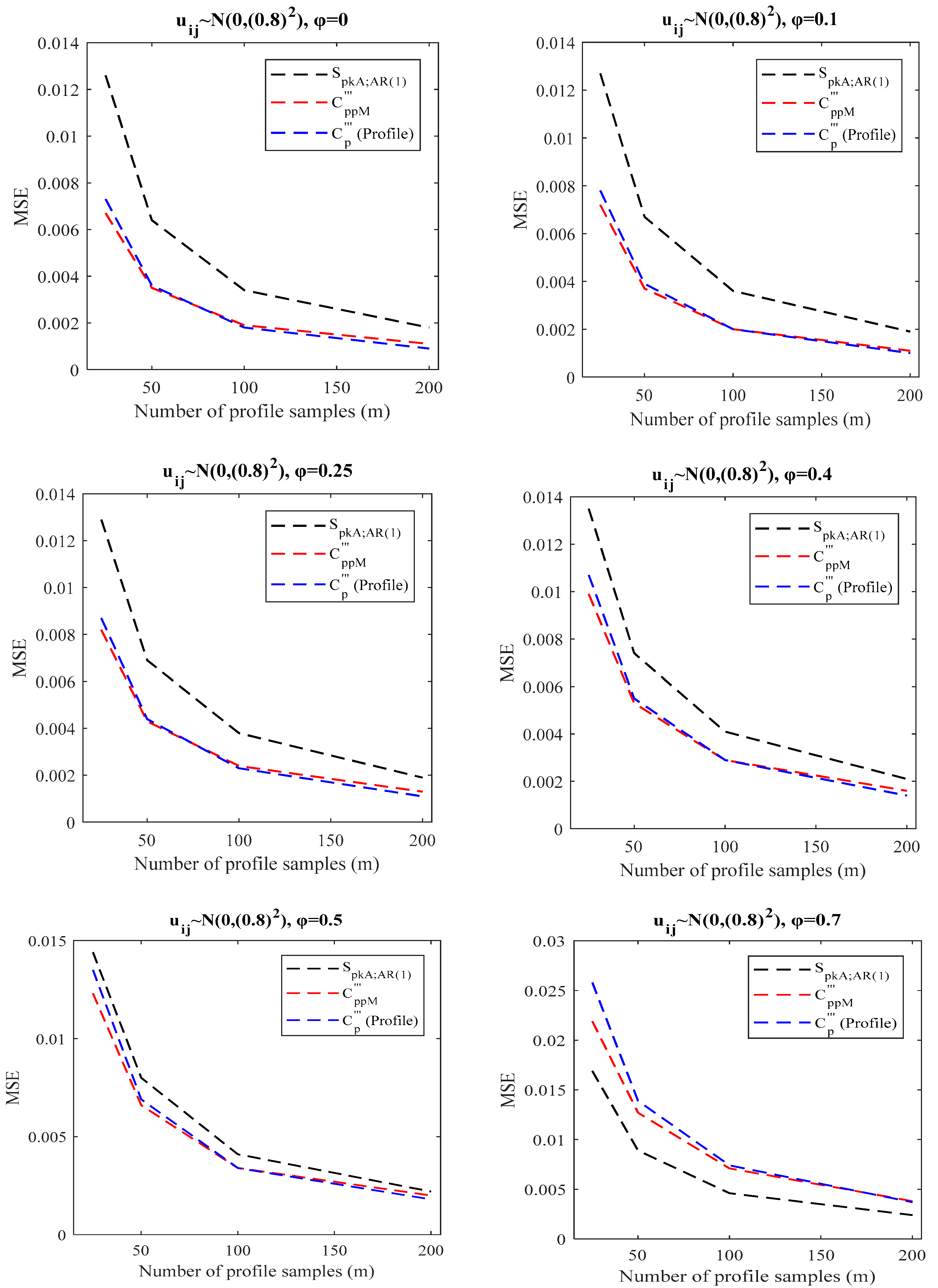
Figure 1. Comparison of various PCIs based on MSE criteria under different profile sample sizes m and parameters φ for SLP with BPAC when u i j ~ N ( 0 , 0.8 2 ) .
Mathematics 12 02549 g001
Figure 2. Comparison of various PCIs based on MSE criteria under different profile sample sizes m and parameters φ for SLP with BPAC when u i j ~ N ( 0 , 1.0 2 ) .
Mathematics 12 02549 g002
Figure 3. Comparison of various PCIs based on MSE criteria under different profile sample sizes m and parameters φ for SLP with BPAC when u i j ~ N ( 0 , 1.2 2 ) .
Mathematics 12 02549 g003
Figure 4. Comparison of various PCIs based on MSE criteria under different profile sample sizes m and parameters ρ for SLP with WPAC when u i j ~ N ( 0 , 0.8 2 ) .
Mathematics 12 02549 g004
Figure 5. Comparison of various PCIs based on MSE criteria under different profile sample sizes m and parameters ρ for SLP with WPAC when u i j ~ N ( 0 , 1.0 2 ) .
Mathematics 12 02549 g005
Figure 6. Comparison of various PCIs based on MSE criteria under different profile sample sizes m and parameters ρ for SLP with WPAC when u i j ~ N ( 0 , 1.2 2 ) .
Mathematics 12 02549 g006
Figure 7. MSE of the proposed index in Section 3 (solid lines) and Section 3 (dotted lines) under different profile sample sizes m and φ = 0.1 (black lines),   φ = 0.25 (blue lines), φ = 0.4 (red lines), φ = 0.5 (green lines), and   φ = 0.7 (yellow lines) when there is a BPAC effect.
Mathematics 12 02549 g007
Figure 8. The transformed functional limits of the calibration of metal oxide (MOX) data.
Mathematics 12 02549 g008
Table 1. SLs for each level of the explanatory variable based on Wang and Tamirat [35].
i 12345678910
X i 12345678910
L S L i 0.082.54.646.859.211.2513.7616.2518.3219.5
U S L i 7.581012.1414.3516.718.7521.2623.7525.8227
T i 3.836.258.3910.612.951517.512022.0723.25
Table 2. A comparison among S p k A ; A R ( 1 ) , C p p M , and C p ( P r o f i l e ) for SLP with BPAC when u i j ~ N ( 0 , 0.8 2 ) .
φ m S p k A ; A R ( 1 ) C p p M C p ( P r o f i l e )
True ValueEstimate
(Bias, MSE)
True ValueEstimate
(Bias, MSE)
True ValueEstimate
(Bias, MSE)
0251.29711.2589
(−0.0382, 0.0126)
1.23631.2184
(−0.0179, 0.0067)
1.31601.3162
(0.0002, 0.0073)
501.2780
(−0.0191, 0.0064)
1.2193
(−0.0170, 0.0035)
1.3166
(0.0006, 0.0036)
1001.2867
(−0.0104, 0.0034)
1.2190
(−0.0173, 0.0019)
1.3158
(−0.0002, 0.0018)
2001.2917
(−0.0054, 0.0018)
1.2187
(−0.0176, 0.0011)
1.3154
(−0.0006, 0.0009)
0.1251.29161.2576
(−0.0340, 0.0127)
1.23631.2180
(−0.0183, 0.0072)
1.31601.3151
(−0.0009, 0.0078)
501.2738
(−0.0178, 0.0067)
1.2190
(−0.0173, 0.0037)
1.3158
(−0.0002, 0.0039)
1001.2826
(−0.0090, 0.0036)
1.2194
(−0.0169, 0.0020)
1.3160
(0.0000, 0.0020)
2001.2880
(−0.0036, 0.0019)
1.2198
(−0.0165, 0.0011)
1.3163
(0.0003, 0.0010)
0.25251.26241.2328
(−0.0296, 0.0129)
1.23631.2152
(−0.0211, 0.0082)
1.31601.3107
(0.0053, 0.0087)
501.2461
(−0.0163, 0.0069)
1.2182
(−0.0181, 0.0043)
1.3141
(0.0019, 0.0044)
1001.2540
(−0.0084, 0.0038)
1.2184
(−0.0179, 0.0024)
1.3145
(−0.0015, 0.0023)
2001.2582
(−0.0042, 0.0019)
1.2190
(−0.0173, 0.0013)
1.3154
(−0.0006, 0.0011)
0.4251.20581.1858
(−0.0200, 0.0135)
1.23631.2148
(−0.0215, 0.0099)
1.31601.3077
(0.0083, 0.0107)
501.1944
(−0.0114, 0.0074)
1.2177
(−0.0186, 0.0053)
1.3120
(0.0040, 0.0055)
1001.1986
(−0.0072, 0.0041)
1.2186
(−0.0177, 0.0029)
1.3139
(−0.0021, 0.0029)
2001.2019
(−0.0039, 0.0021)
1.2188
(−0.0175, 0.0016)
1.3148
(−0.0012, 0.0014)
0.5251.15031.1391
(−0.0112, 0.0144)
1.23631.2130
(−0.0233, 0.0123)
1.31601.3027
(−0.0133, 0.0135)
501.1424
(−0.0079, 0.0080)
1.2178
(−0.0185, 0.0066)
1.3104
(−0.0056, 0.0069)
1001.1450
(−0.0053, 0.0041)
1.2187
(−0.0176, 0.0034)
1.3129
(−0.0031, 0.0034)
2001.1466
(−0.0037, 0.0022)
1.2187
(−0.0176, 0.0020)
1.3138
(−0.0022, 0.0018)
0.7250.98020.9974
(0.0172, 0.0169)
1.23631.1995
(−0.0368, 0.0219)
1.31601.2742
(−0.0418, 0.0258)
500.9840
(0.0038, 0.0089)
1.2095
(−0.0268, 0.0127)
1.2934
(−0.0226, 0.0139)
1000.9788
(−0.0014, 0.0046)
1.2139
(−0.0224, 0.0071)
1.3035
(−0.0125, 0.0074)
2000.9792
(−0.0010, 0.0024)
1.2174
(−0.0189, 0.0038)
1.3101
(−0.0059, 0.0037)
Note: Bold values indicate the best-performing index in terms of Bias and MSE for each simulated case.
Table 3. A comparison among S p k A ; A R ( 1 ) , C p p M , and C p ( P r o f i l e ) for SLP with BPAC when u i j ~ N ( 0 , 1.0 2 ) .
φ m S p k A ; A R ( 1 ) C p p M C p ( P r o f i l e )
True ValueEstimated
(Bias, MSE)
True ValueEstimated
(Bias, MSE)
True ValueEstimated
(Bias, MSE)
0251.07711.0488
(−0.0283, 0.0071)
1.04461.0254
(−0.0192, 0.0053)
1.10481.1042
(−0.0006, 0.0056)
501.0629
(−0.0142, 0.0037)
1.0270
(−0.0176, 0.0028)
1.1050
(0.0002, 0.0028)
1001.0696
(−0.0075, 0.0009)
1.0270
(−0.0176, 0.0007)
1.1048
(0.0000, 0.0008)
2001.0738
(−0.0033, 0.0010)
1.0275
(−0.0171, 0.0009)
1.1050
(0.0002, 0.0007)
0.1251.07261.0474
(−0.0252, 0.0075)
1.04461.0251
(−0.0195, 0.0058)
1.10481.1032
(0.0016, 0.0061)
501.0581
(−0.0145 0.0038)
1.0260
(−0.0186, 0.0030)
1.1039
(−0.0009, 0.0030)
1001.0655
(−0.0071, 0.0019)
1.0269
(−0.0177, 0.0017)
1.1045
(−0.0003, 0.0015)
2001.0686
(−0.0040, 0.0010)
1.0267
(−0.0179, 0.0010)
1.1042
(−0.0006, 0.0008)
0.25251.04861.0270
(−0.0216, 0.0077)
1.04461.0230
(−0.0216, 0.0065)
1.10481.0998
(−0.0050, 0.0067)
501.0375
(−0.0111, 0.0041)
1.0261
(−0.0185, 0.0034)
1.1030
(−0.0018, 0.0033)
1001.0424
(−0.0062, 0.0022)
1.0265
(−0.0181, 0.0019)
1.1037
(−0.0011, 0.0017)
2001.0459
(0.0027, 0.0011)
1.0273
(−0.0173, 0.0011)
1.1045
(−0.0003, 0.0009)
0.4251.00190.9876
(−0.0143, 0.0085)
1.04461.0208
(−0.0238, 0.0082)
1.10481.0950
(0.0098, 0.0083)
500.9921
(−0.0098, 0.0044)
1.0239
(−0.0207, 0.0043)
1.0995
(−0.0053, 0.0041)
1000.9967
(−0.0052, 0.0023)
1.0257
(−0.0189, 0.0024)
1.1022
(−0.0026, 0.0021)
2000.9986
(−0.0033, 0.0012)
1.0261
(−0.0185, 0.0013)
1.1030
(−0.0018, 0.0010)
0.5250.95580.9469
(−0.0089, 0.0090)
1.04461.0183
(−0.0263, 0.0096)
1.10481.0899
(−0.0149, 0.0098)
500.9491
(−0.0067, 0.0048)
1.0226
(−0.0220, 0.0054)
1.0964
(−0.0084, 0.0050)
1000.9519
(−0.0039, 0.0025)
1.0250
(−0.0196, 0.0029)
1.1005
(−0.0043, 0.0025)
2000.9531
(−0.0027, 0.0013)
1.0260
(−0.0186, 0.0016)
1.1023
(−0.0025, 0.0013)
0.7250.81250.8247
(0.0122, 0.0104)
1.04460.9973
(−0.0473, 0.0170)
1.10481.0564
(−0.0484, 0.0189)
500.8164
(0.0039, 0.0054)
1.0123
(−0.0232, 0.0097)
1.0781
(−0.0267, 0.0098)
1000.8135
(0.0010, 0.0028)
1.0203
(−0.0243, 0.0053)
1.0909
(−0.0139, 0.0049)
2000.8124
(−0.0001, 0.0014)
1.0244
(−0.0202, 0.0030)
1.0981
(−0.0067, 0.0025)
Note: Bold values indicate the best-performing index in terms of Bias and MSE for each simulated case.
Table 4. A comparison among S p k A ; A R ( 1 ) , C p p M , and C p ( P r o f i l e ) for SLP with BPAC when u i j ~ N ( 0 , 1.2 2 ) .
φ m S p k A ; A R ( 1 ) C p p M C p ( P r o f i l e )
True ValueEstimated
(Bias, MSE)
True ValueEstimated
(Bias, MSE)
True ValueEstimated
(Bias, MSE)
0250.92550.9041
(−0.0214, 0.0046)
0.90250.8828
(−0.0197, 0.0043)
0.94770.9465
(−0.0012, 0.0044)
500.9149
(−0.0106, 0.0023)
0.9096
(−0.0178, 0.0023)
0.9475
(−0.0002, 0.0022)
1000.9199
(−0.0056, 0.0012)
0.8850
(−0.0175, 0.0013)
0.9474
(−0.0003, 0.0011)
2000.9231
(−0.0024, 0.0006)
0.8855
(−0.0170, 0.0008)
0.9478
(0.0001, 0.0005)
0.1250.92170.9024
(−0.0193, 0.0050)
0.90250.8823
(−0.0202, 0.0048)
0.94770.9453
(−0.0024, 0.0048)
500.9108
(−0.0109, 0.0025)
0.8837
(−0.0188, 0.0025)
0.9465
(−0.0012, 0.0023)
1000.9167
(−0.0050, 0.0013)
0.8850
(−0.0175, 0.0014)
0.9473
(−0.0004, 0.0011)
2000.9193
(−0.0024, 0.0006)
0.8854
(−0.0171, 0.0008)
0.9476
(−0.0001, 0.0006)
0.25250.90090.8847
(−0.0162, 0.0051)
0.90250.8802
(−0.0223, 0.0054)
0.94770.9420
(−0.0057, 0.0052)
500.8916
(−0.0093, 0.0027)
0.8831
(−0.0194, 0.0028)
0.9449
(−0.0028, 0.0026)
1000.8962
(−0.0047, 0.0014)
0.8841
(−0.0184, 0.0016)
0.9462
(−0.0015, 0.0013)
2000.8981
(−0.0028, 0.0007)
0.8845
(−0.0180, 0.0010)
0.9466
(−0.0011, 0.0006)
0.4250.86020.8504
(−0.0098, 0.0055)
0.90250.8774
(−0.0251, 0.0065)
0.94770.9370
(−0.0107, 0.0063)
500.8534
(−0.0068, 0.0030)
0.8813
(−0.0212, 0.0035)
0.9419
(−0.0058, 0.0031)
1000.8570
(−0.0032, 0.0015)
0.8837
(−0.0188, 0.0019)
0.9450
(−0.0027, 0.0015)
2000.8575
(−0.0027, 0.0008)
0.8839
(−0.0186, 0.0011)
0.9457
(−0.0020, 0.0008)
0.5250.81980.8148
(−0.0050, 0.0062)
0.90250.8729
(−0.0296, 0.0079)
0.94770.9304
(0.0173, 0.0076)
500.8156
(−0.0042, 0.0031)
0.8794
(−0.0231, 0.0041)
0.9387
(−0.0090, 0.0036)
1000.8176
(−0.0022, 0.0016)
0.8826
(−0.0199, 0.0023)
0.9431
(−0.0046, 0.0018)
2000.8181
(−0.0017, 0.0009)
0.8836
(−0.0189, 0.0013)
0.9449
(−0.0028, 0.0009)
0.7250.69390.7061
(0.0122, 0.0073)
0.90250.8486
(−0.0539, 0.0143)
0.94770.8969
(−0.0508, 0.0151)
500.6989
(0.0050, 0.0038)
0.8666
(−0.0359, 0.0080)
0.9197
(−0.0280, 0.0075)
1000.6964
(0.0025, 0.0020)
0.8750
(−0.0275, 0.0044)
0.9320
(−0.0157, 0.0037)
2000.6949
(0.0010, 0.0010)
0.8812
(−0.0213, 0.0024)
0.9403
(−0.0074, 0.0018)
Note: Bold values indicate the best-performing index in terms of Bias and MSE for each simulated case.
Table 5. A comparison among S p k A ; A R ( 1 ) , C p p M , and C p ( P r o f i l e ) for SLP with WPAC when u i j ~ N ( 0 , 0.8 2 ) .
ρ m S p k A ; A R ( 1 ) C p p M C p ( P r o f i l e )
True ValueEstimated
(Bias, MSE)
True ValueTrue ValueEstimated
(Bias, MSE)
True Value
0251.26311.2071
(−0.0560, 0.0078)
1.26131.2563
(−0.0050, 0.0036)
1.31711.3184
(0.0013, 0.0043)
501.2313
(−0.0318, 0.0037)
1.2562
(−0.0051, 0.0018)
1.3175
(0.0004, 0.0021)
1001.2467
(−0.0164, 0.0017)
1.2564
(−0.0049, 0.0009)
1.3174
(0.0003, 0.0010)
2001.2546
(−0.0085, 0.0008)
1.2560
(−0.0053, 0.0005)
1.3170
(−0.0001, 0.0005)
0.1251.25791.2025
(−0.0554, 0.0078)
1.1661.1601
(−0.0059, 0.0031)
1.22381.2243
(0.0005, 0.0038)
501.2267
(−0.0312, 0.0037)
1.1601
(−0.0059, 0.0016)
1.2236
(0.0002, 0.0019)
1001.2413
(−0.0166, 0.0017)
1.1606
(−0.0054, 0.0008)
1.2238
(0.0000, 0.0009)
2001.2493
(−0.0086, 0.0008)
1.1611
(−0.0049, 0.0004)
1.2242
(0.0004, 0.0005)
0.25251.23051.1787
(−0.0518, 0.0072)
1.00520.9992
(−0.0060, 0.0024)
1.06471.0650
(0.0003, 0.0031)
501.2018
(−0.0287, 0.0034)
1.0000
(−0.0052, 0.0012)
1.0651
(0.0004, 0.0015)
1001.2151
(−0.0154, 0.0017)
0.9999
(−0.0053, 0.0006)
1.0646
(−0.0001, 0.0008)
2001.2229
(−0.0076, 0.0008)
1.0006
(−0.0046, 0.0003)
1.0652
(0.0005, 0.0004)
0.4251.17711.1320
(−0.0451, 0.0065)
0.82260.8168
(−0.0058, 0.0016)
0.88180.8814
(−0.0004, 0.0023)
501.1522
(−0.0249, 0.0032)
0.8172
(−0.0054, 0.0008)
0.8812
(0.0006, 0.0011)
1001.1639
(−0.0132, 0.0015)
0.8179
(−0.0047, 0.0004)
0.8817
(−0.0001, 0.0006)
2001.1703
(−0.0068, 0.0007)
0.8181
(−0.0045, 0.0002)
0.8818
(−0.0000, 0.0003)
0.5251.12471.0859
(−0.0388, 0.0057)
0.68920.6839
(−0.0053, 0.0011)
0.74730.7468
(−0.0005, 0.0017)
501.1031
(−0.0216, 0.0029)
0.6848
(−0.0044, 0.0006)
0.7472
(−0.0001, 0.0008)
1001.1136
(−0.0111, 0.0013)
0.6851
(−0.0041, 0.0003)
0.7471
(0.0002, 0.0004)
2001.1187
(−0.0060, 0.0007)
0.6852
(−0.0040, 0.0002)
0.7472
(−0.0001, 0.0002)
0.7250.96320.9383
(−0.0249, 0.0044)
0.3950.3912
(−0.0038, 0.0004)
0.45320.4517
(0.0015, 0.0007)
500.9504
(−0.0128, 0.0022)
0.3921
(−0.0029, 0.0002)
0.4525
(−0.0007, 0.0003)
1000.9566
(−0.0066, 0.0011)
0.3924
(−0.0026, 0.0001)
0.4527
(−0.0005, 0.0002)
2000.9595
(−0.0037, 0.0006)
0.3927
(−0.0023, 0.0001)
0.4530
(−0.0002, 0.0001)
Note: Bold values indicate the best-performing index in terms of Bias and MSE for each simulated case.
Table 6. A comparison among S p k A ; A R ( 1 ) , C p p M , and C p ( P r o f i l e ) for SLP with WPAC when u i j ~ N ( 0 , 1.0 2 ) .
ρ m S p k A ; A R ( 1 ) C p p M C p ( P r o f i l e )
True ValueEstimated
(Bias, MSE)
True ValueEstimated
(Bias, MSE)
True ValueEstimated
(Bias, MSE)
0251.05531.0171
(−0.0382, 0.0040)
1.06111.0559
(−0.0052, 0.0027)
1.10531.1059
(0.0006, 0.0032)
501.0345
(−0.0208, 0.0019)
1.0563
(−0.0048, 0.0014)
1.1058
(0.0005, 0.0016)
1001.0447
(−0.0106, 0.0009)
1.0563
(−0.0048, 0.0007)
1.1055
(0.0002, 0.0008)
2001.0493
(−0.0060, 0.0004)
1.0563
(−0.0048, 0.0004)
1.1053
(0.0000, 0.0004)
0.1251.05111.0127
(−0.0384, 0.0041)
0.97470.9681
(−0.0066, 0.0024)
1.01811.0173
(0.0008, 0.0028)
501.0306
(−0.0205 0.0018)
0.9697
(−0.0050, 0.0012)
1.0183
(0.0002, 0.0014)
1001.0404
(−0.0107, 0.0009)
0.9700
(−0.0047, 0.0006)
1.0183
(0.0002, 0.0007)
2001.0460
(−0.0051, 0.0004)
0.9701
(−0.0046, 0.0003)
1.0182
(0.0001, 0.0004)
0.25251.02830.9931
(−0.0352, 0.0038)
0.8330.8267
(−0.0063, 0.0018)
0.87470.8737
(−0.0010, 0.0022)
501.0094
(−0.0189, 0.0018)
0.8282
(−0.0048, 0.0009)
0.8749
(0.0002, 0.0011)
1001.0186
(−0.0097, 0.0009)
0.8283
(−0.0047, 0.0005)
0.8746
(−0.0001, 0.0005)
2001.0230
(0.0053, 0.0004)
0.8287
(−0.0043, 0.0002)
0.8747
(0.0001, 0.0003)
0.4250.98390.9530
(−0.0309, 0.0036)
0.6770.6720
(−0.0050, 0.0012)
0.71690.7165
(−0.0004, 0.0015)
500.9675
(−0.0164, 0.0017)
0.6719
(−0.0051, 0.0006)
0.7160
(−0.0009, 0.0008)
1000.9754
(−0.0085, 0.0008)
0.6728
(−0.0042, 0.0003)
0.7167
(−0.0002, 0.0004)
2000.9791
(−0.0048, 0.0004)
0.6733
(0.0037, 0.0002)
0.7170
(0.0001, 0.0002)
0.5250.93980.9132
(−0.0266, 0.0033)
0.56530.5601
(−0.0052, 0.0009)
0.60440.6031
(−0.0013, 0.0011)
500.9261
(−0.0137, 0.0016)
0.5615
(−0.0038, 0.0004)
0.6042
(−0.0002, 0.0006)
1000.9325
(−0.0073, 0.0008)
0.5614
(−0.0039, 0.0002)
0.6038
(−0.0006, 0.0003)
2000.9363
(−0.0035, 0.0004)
0.5622
(−0.0031, 0.0001)
0.6045
(0.0001, 0.0001)
0.7250.80230.7862
(−0.0161, 0.0028)
0.32270.3183
(−0.0044, 0.0003)
0.36470.3621
(−0.0026, 0.0005)
500.7937
(−0.0086, 0.0015)
0.3197
(−0.0031, 0.0002)
0.3633
(−0.0014, 0.0002)
1000.7984
(−0.0039, 0.0007)
0.3202
(−0.0025, 0.0001)
0.3640
(−0.0007, 0.0001)
2000.8003
(−0.0020, 0.0004)
0.3206
(−0.0021, 0.0000)
0.3644
(−0.0003, 0.0001)
Note: Bold values indicate the best-performing index in terms of Bias and MSE for each simulated case.
Table 7. A comparison among S p k A ; A R ( 1 ) , C p p M , and C p ( P r o f i l e ) for SLP with WPAC when u i j ~ N ( 0 , 1.2 2 ) .
ρ m S p k A ; A R ( 1 ) C p p M C p ( P r o f i l e )
True ValueEstimated
(Bias, MSE)
True ValueEstimated
(Bias, MSE)
True ValueEstimated
(Bias, MSE)
0250.91090.8832
(−0.0277, 0.0024)
0.91390.9090
(−0.0049, 0.0022)
0.94790.9485
(0.0006, 0.0025)
500.8963
(−0.0146, 0.0011)
0.9096
(−0.0043, 0.0011)
0.9485
(−0.0006, 0.0012)
1000.9034
(−0.0075, 0.0005)
0.9094
(−0.0045, 0.0006)
0.9480
(0.0001, 0.0006)
2000.9072
(−0.0037, 0.0003)
0.9096
(−0.0043, 0.0003)
0.9480
(0.0001, 0.0003)
0.1250.90720.8802
(−0.0270, 0.0024)
0.83570.8302
(−0.0055, 0.0019)
0.86820.8680
(−0.0002, 0.0022)
500.8922
(−0.0150, 0.0011)
0.8306
(−0.0051, 0.0010)
0.8678
(−0.0004, 0.0011)
1000.8997
(−0.0075, 0.0005)
0.8308
(−0.0049, 0.0005)
0.8677
(−0.0005, 0.0006)
2000.9034
(−0.0038, 0.0003)
0.8315
(−0.0042, 0.0003)
0.8683
(0.0001, 0.0003)
0.25250.88730.8612
(−0.0261, 0.0023)
0.70990.7042
(−0.0057, 0.0014)
0.74020.7394
(0.0008, 0.0017)
500.8739
(−0.0134, 0.0011)
0.7056
(−0.0043, 0.0007)
0.7402
(0.0000, 0.0008)
1000.8805
(−0.0068, 0.0005)
0.7057
(−0.0042, 0.0004)
0.7400
(−0.0002, 0.0004)
2000.8840
(−0.0033, 0.0003)
0.7059
(−0.0040, 0.0002)
0.7401
(−0.0001, 0.0002)
0.4250.84820.8249
(−0.0233, 0.0023)
0.57420.5687
(−0.0055, 0.0009)
0.60290.6014
(−0.0015, 0.0011)
500.8366
(−0.0116, 0.0011)
0.5699
(−0.0043, 0.0005)
0.6022
(−0.0007, 0.0006)
1000.8428
(−0.0054, 0.0005)
0.5707
(−0.0035, 0.0002)
0.6028
(−0.0001, 0.0003)
2000.8450
(−0.0032, 0.0003)
0.5707
(−0.0035, 0.0001)
0.6026
(−0.0003, 0.0001)
0.5250.80940.7905
(−0.0189, 0.0022)
0.47840.4735
(−0.0049, 0.0006)
0.50670.5053
(−0.0014, 0.0008)
500.8000
(−0.0094, 0.0011)
0.4744
(−0.0040, 0.0003)
0.5058
(−0.0009, 0.0004)
1000.8041
(−0.0053, 0.0005)
0.4750
(−0.0034, 0.0002)
0.5062
(−0.0005, 0.0002)
2000.8071
(−0.0023, 0.0003)
0.4754
(−0.0030, 0.0001)
0.5065
(−0.0002, 0.0001)
0.7250.68730.6768
(−0.0105, 0.0021)
0.27240.2677
(−0.0047, 0.0003)
0.30490.3018
(−0.0031, 0.0003)
500.6823
(−0.0050, 0.0011)
0.2696
(−0.0028, 0.0001)
0.3037
(−0.0012, 0.0002)
1000.6849
(−0.0024, 0.0006)
0.2700
(−0.0024, 0.0001)
0.3041
(−0.0008, 0.0001)
2000.6860
(−0.0013, 0.0003)
0.2704
(−0.0020, 0.0000)
0.3044
(−0.0005, 0.0000)
Note: Bold values indicate the best-performing index in terms of Bias and MSE for each simulated case.
Table 8. The simulation results of C p ( P r o f i l e ) for SLP with BAC.
Cases   u i j u i j ~ N ( 0 ,   0.8 2 ) u i j ~ N ( 0 ,   1.0 2 ) u i j ~ N ( 0 ,   1.2 2 )
ρ ,   φ m C p ( P r o f i l e ) C ^ p ( P r o f i l e )
(Bias, MSE)
C p ( P r o f i l e ) C ^ p ( P r o f i l e )
(Bias, MSE)
C p ( P r o f i l e ) C ^ p ( P r o f i l e )
(Bias, MSE)
ρ = 0
φ = 0
251.34931.3498
(0.0005, 0.0106)
1.12541.1250
(−0.0004, 0.0081)
0.96140.9603
(−0.0011, 0.0064)
501.3510
(0.0017, 0.0051)
1.1252
(−0.0002, 0.0039)
0.9620
(0.0006, 0.0031)
1001.3499
(0.0006, 0.0026)
1.1255
(0.0001, 0.0019)
0.9606
(−0.0008, 0.0015)
2001.3496
(0.0003, 0.0013)
1.1254
(0.0000, 0.0010)
0.9615
(0.0001, 0.0008)
ρ = 0.1
φ = 0.1
251.13871.1378
(−0.0009, 0.0085)
0.93830.9370
(−0.0013, 0.0062)
0.79550.7937
(−0.0018, 0.0046)
501.1398
(0.0011, 0.0043)
0.9386
(0.0003, 0.0030)
0.7945
(−0.0010, 0.0022)
1001.1388
(0.0001, 0.0021)
0.9383
(−0.0000, 0.0015)
0.7949
(−0.0006, 0.0011)
2001.1388
(0.0001, 0.0011)
0.9386
(0.0003, 0.0008)
0.7951
(−0.0004, 0.0006)
ρ = 0.25
φ = 0.25
250.80370.8016
(−0.0021, 0.0048)
0.65740.6545
(−0.0029, 0.0035)
0.55490.5507
(−0.0042, 0.0025)
500.8029
(−0.0008, 0.0024)
0.6559
(−0.0015, 0.0016)
0.5532
(−0.0017, 0.0012)
1000.8032
(−0.0005, 0.0012)
0.6569
(−0.0005, 0.0008)
0.5546
(−0.0003, 0.0006)
2000.8031
(−0.0006, 0.0006)
0.6568
(−0.0006, 0.0004)
0.5545
(−0.0004, 0.0003)
ρ = 0.4
φ = 0.4
250.51610.5118
(−0.0043, 0.0025)
0.41960.4145
(−0.0051, 0.0017)
0.35290.3466
(−0.0063, 0.0014)
500.5146
(−0.0015, 0.0012)
0.4172
(−0.0024, 0.0008)
0.3499
(−0.0030, 0.0006)
1000.5147
(−0.0014, 0.0006)
0.4182
(−0.0014, 0.0004)
0.3514
(−0.0015, 0.0003)
2000.5158
(−0.0003, 0.0003)
0.4189
(−0.0007, 0.0002)
0.3522
(−0.0007, 0.0002)
ρ = 0.5
φ = 0.5
250.35520.3479
(−0.0073, 0.0016)
0.28770.2798
(−0.0079, 0.0012)
0.24140.2315
(−0.0099, 0.0011)
500.3516
(−0.0036, 0.0008)
0.2836
(−0.0041, 0.0006)
0.2362
(−0.0052, 0.0005)
1000.3536
(−0.0016, 0.0004)
0.2855
(−0.0022, 0.0003)
0.2390
(−0.0024, 0.0002)
2000.3543
(−0.0009, 0.0002)
0.2868
(−0.0009, 0.0001)
0.2401
(−0.0013, 0.0001)
ρ = 0.7
φ = 0.7
250.11280.0946
(−0.0182, 0.0018)
0.09080.0685
(−0.0223, 0.0021)
0.07590.0501
(−0.0258, 0.0024)
500.1033
(−0.0095, 0.0008)
0.0792
(−0.0116, 0.0009)
0.0627
(−0.0132, 0.0009)
1000.1076
(−0.0052, 0.0004)
0.0850
(−0.0058, 0.0004)
0.0691
(−0.0068, 0.0004)
2000.1103
(−0.0025, 0.0002)
0.0879
(−0.0029, 0.0002)
0.0724
(−0.0035, 0.0002)
ρ = 0
φ = 0
251.37371.3734
(−0.0003, 0.0109)
1.14091.1430
(0.0021, 0.0084)
0.97190.9690
(−0.0029, 0.0063)
501.3734
(−0.0003, 0.0054)
1.1411
(0.0002, 0.0040)
0.9709
(−0.0010, 0.0031)
1001.3745
(−0.0008, 0.0026)
1.1405
(−0.0004, 0.0020)
0.9713
(−0.0006, 0.0015)
2001.3733
(−0.0004, 0.0013)
1.1409
(0.0000, 0.0010)
0.9714
(−0.0005, 0.0008)
ρ = 0.1
φ = 0.1
251.16751.1659
(−0.0020, 0.0088)
0.95590.9544
(−0.0015, 0.0065)
0.80720.8052
(−0.0020, 0.0047)
501.1674
(−0.0005, 0.0043)
0.9562
(0.0003 0.0031)
0.8060
(−0.0012, 0.0022)
1001.1685
(0.0006, 0.0022)
0.9550
(−0.0009, 0.0015)
0.8065
(−0.0007, 0.0011)
2001.1677
(−0.0002, 0.0011)
0.9559
(0.0000, 0.0008)
0.8067
(−0.0005, 0.0006)
ρ = 0.25
φ = 0.25
250.82190.8195
(−0.0024, 0.0049)
0.66880.6653
(−0.0035, 0.0034)
0.56270.5595
(−0.0032, 0.0025)
500.8209
(−0.0010, 0.0024)
0.6668
(−0.0020, 0.0017)
0.5608
(−0.0019, 0.0012)
1000.8212
(−0.0007 0.0012)
0.6679
(−0.0009, 0.0008)
0.5614
(−0.0013, 0.0006)
2000.8214
(−0.0005, 0.0006)
0.6683
(−0.0005, 0.0004)
0.5621
(−0.0006, 0.0003)
ρ = 0.4
φ = 0.4
250.52610.5221
(−0.0040, 0.0024)
0.42630.4210
(−0.0053, 0.0017)
0.35780.3510
(−0.0068, 0.0013)
500.5241
(−0.0020, 0.0012)
0.4238
(−0.0025, 0.0008)
0.3546
(−0.0032, 0.0006)
1000.5250
(−0.0011, 0.0006)
0.4247
(−0.0016, 0.0004)
0.3562
(−0.0016, 0.0003)
2000.5256
(−0.0005, 0.0003)
0.4256
(−0.0007, 0.0002)
0.3572
(−0.0006, 0.0001)
ρ = 0.5
φ = 0.5
250.36180.3549
(−0.0069, 0.0015)
0.29240.2843
(−0.0081, 0.0012)
0.24500.2351
(−0.0099, 0.0010)
500.3584
(−0.0034, 0.0007)
0.2883
(−0.0041, 0.0006)
0.2400
(−0.0050, 0.0004)
1000.3597
(−0.0021, 0.0004)
0.2902
(−0.0022, 0.0003)
0.2426
(−0.0024, 0.0002)
2000.3608
(−0.0010, 0.0002)
0.2913
(−0.0011, 0.0001)
0.2439
(−0.0011, 0.0001)
ρ = 0.7
φ = 0.7
250.11600.0973
(−0.0187, 0.0018)
0.09330.0711
(−0.0222, 0.0020)
0.07790.0510
(−0.0269, 0.0024)
500.1067
(−0.0093, 0.0007)
0.0823
(−0.0110, 0.0008)
0.0646
(−0.0133, 0.0009)
1000.1117
(−0.0043, 0.0003)
0.0872
(−0.0061, 0.0003)
0.0710
(−0.0069, 0.0004)
2000.1138
(−0.0022, 0.0002)
0.0905
(−0.0028, 0.0001)
0.0745
(−0.0034, 0.0002)
Table 9. The simulation results of C p ( P r o f i l e ) for SLP with BAC when there is a BPAC effect.
Cases   u i j u i j ~ N ( 0 , 1.2 2 ) u i j ~ N ( 0 , 1.0 2 ) u i j ~ N ( 0 , 0.8 2 )
m ρ , φ C p ( P r o f i l e ) C ^ p ( P r o f i l e )
(Bias, MSE)
C p ( P r o f i l e ) C ^ p ( P r o f i l e )
(Bias, MSE)
C p ( P r o f i l e ) C ^ p ( P r o f i l e )
(Bias, MSE)
ρ = 0
φ = 0.1
251.26671.2682
(0.0015, 0.0103)
1.04431.0433
(−0.0010, 0.0073)
0.88560.8835
(−0.0021, 0.0055)
501.2655
(−0.0012, 0.0050)
1.0450
(−0.0007, 0.0036)
0.8850
(−0.0006, 0.0027)
1001.2666
(−0.0001, 0.0025)
1.0439
(−0.0004, 0.0018)
0.8851
(−0.0005, 0.0013)
2001.2666
(−0.0001, 0.0012)
1.0442
(−0.0001, 0.0009)
0.8853
(−0.0003, 0.0007)
ρ = 0
φ = 0.25
251.08271.0809
(−0.0018, 0.0081)
0.88560.8829
(−0.0027, 0.0055)
0.74750.7451
(−0.0024, 0.0041)
501.0814
(0.0013, 0.0039)
0.8845
(−0.0011, 0.0028)
0.7458
(−0.0017, 0.0020)
1001.0816
(−0.0011, 0.0019)
0.8847
(−0.0009, 0.0013)
0.7472
(−0.0003, 0.0010)
2001.0827
(0.0000, 0.0010)
0.8852
(−0.0004, 0.0006)
0.7472
(−0.0003, 0.0005)
ρ = 0
φ = 0.4
250.88560.8808
(−0.0048, 0.0056)
0.71920.7140
(−0.0052, 0.0037)
0.60450.5985
(−0.0060, 0.0028)
500.8829
(−0.0027, 0.0027)
0.7170
(−0.0022, 0.0019)
0.6012
(−0.0033, 0.0014)
1000.8844
(−0.0012, 0.0014)
0.7178
(−0.0014, 0.0009)
0.6033
(−0.0012, 0.0006)
2000.8850
(−0.0006, 0.0007)
0.7184
(−0.0008, 0.0005)
0.6036
(−0.0009, 0.0003)
ρ = 0
φ = 0.5
250.74750.7413
(−0.0062, 0.0040)
0.60450.5973
(−0.0072, 0.0028)
0.50680.5007
(−0.0061, 0.0021)
500.7446
(−0.0029, 0.0020)
0.6011
(−0.0034, 0.0013)
0.5032
(−0.0036, 0.0010)
1000.7455
(−0.0020, 0.0010)
0.6028
(−0.0017, 0.0006)
0.5047
(−0.0021, 0.0005)
2000.7465
(−0.0010, 0.0005)
0.6034
(−0.0011, 0.0003)
0.5058
(−0.0010, 0.0002)
ρ = 0
φ = 0.7
250.45730.4447
(−0.0126, 0.0018)
0.36730.3549
(−0.0124, 0.0013)
0.30680.2936
(−0.0132, 0.0011)
500.4509
(−0.0064, 0.0009)
0.3605
(−0.0068, 0.0006)
0.3001
(−0.0067, 0.0005)
1000.4539
(−0.0034, 0.0004)
0.3640
(−0.0033, 0.0003)
0.3035
(−0.0033, 0.0002)
2000.4555
(−0.0018, 0.0002)
0.3657
(−0.0016, 0.0001)
0.3052
(−0.0016, 0.0001)
Table 10. The simulation results of 95% bootstrap confidence intervals of C p ( P r o f i l e ) for SLP with BAC.
Simulated Case m True Value
C p ( P r o f i l e )
Estimated
C p ( P r o f i l e )
Bootstrap Methods
SBPB
C I ¯ Relative Coverage C I ¯ Relative Coverage
Y i j = 3 + 2   X i + ε i j
i = 4 ,   ε i j ~ N ( 0 , 1.0 2 )
ρ = φ = 0
251.12541.126(0.9559, 1.2961)2.7597(0.9676, 1.3074)2.7697
501.125(1.0028, 1.2472)3.8175(1.0085, 1.2527)3.841
1001.1265(1.0404, 1.2125)5.4931(1.0430, 1.2148)5.4885
2001.125(1.0641, 1.1860)7.7768(1.0653, 1.1871)7.7838
Y i j = 3 + 2   X i + ε i j
i = 4 ,   ε i j ~ N ( 0 , 1.0 2 )
ρ = φ = 0 .1
250.93830.9363(0.7865, 1.0862)3.1168(0.7968, 1.0960)3.1081
500.9362(0.8294, 1.0429)4.4216(0.8343, 1.0476)4.4357
1000.9384(0.8629, 1.0140)6.2252(0.8650, 1.0141)6.2287
2000.9378(0.8843, 0.9913)8.8712(0.8855, 0.9924)8.9038
Y i j = 3 + 2   X i + ε i j
i = 4 ,   ε i j ~ N ( 0 , 1.0 2 )
ρ = φ = 0 .25
250.65740.6526(0.5409, 0.7642)4.1776(0.5471, 0.7706)4.1787
500.6552(0.5757, 0.7346)5.9732(0.5787, 0.7375)5.9371
1000.6576(0.6012, 0.7141)8.4542(0.6025, 0.7154)8.3983
2000.6563(0.6168, 0.6959)11.958(0.6174, 0.6966)11.9074
Y i j = 3 + 2   X i + ε i j
i = 4 ,   ε i j ~ N ( 0 , 1.0 2 )
ρ = φ = 0 .4
250.41960.4098(0.3282, 0.4913)5.8561(0.3291, 0.4930)5.7814
500.4154(0.3582, 0.4725)8.2756(0.3586, 0.4732)8.2351
1000.4176(0.3776, 0.4577)11.78(0.3775, 0.4578)11.6992
2000.4185(0.3902, 0.4467)16.7696(0.3902, 0.4467)16.7651
Y i j = 3 + 2   X i + ε i j
i = 4 ,   ε i j ~ N ( 0 , 1.0 2 )
ρ = φ = 0.5
250.28770.2736(0.2050, 0.3423)6.947(0.2011, 0.3396)6.8325
500.2798(0.2319, 0.3277)10.0152(0.2296, 0.3258)9.8405
1000.2846(0.2514, 0.3177)14.4352(0.2501, 0.3166)14.256
2000.2858(0.2627, 0.3089)20.6014(0.2620, 0.3082)20.4173
Y i j = 3 + 2   X i + ε i j
i = 4 ,   ε i j ~ N ( 0 , 0.8 2 )
ρ = φ = 0
251.34931.3525(1.1582, 1.5468)2.4161(1.1708, 1.5586)2.4213
501.3496(1.2099, 1.4892)3.3189(1.2160, 1.4951)3.3462
1001.3517(1.2527, 1.4507)4.8505(1.2555, 1.4532)4.8264
2001.3492(1.2792, 1.4191)6.7634(1.2806, 1.4203)6.7917
Y i j = 3 + 2   X i + ε i j
i = 4 ,   ε i j ~ N ( 0 , 0.8 2 )
ρ = φ = 0 .1
251.13871.1528(0.9737, 1.3319)2.5883(0.9859, 1.3433)2.5934
501.1383(1.0120, 1.2646)3.7252(1.0177, 1.2701)3.7207
1001.1396(1.0504, 1.2288)5.2973(1.0528, 1.2311)5.2956
2001.1385(1.0753, 1.2017)7.5008(1.0766, 1.2029)7.5217
Y i j = 3 + 2   X i + ε i j
i = 4 ,   ε i j ~ N ( 0 , 1.2 2 )
ρ = φ = 0
250.96140.9659(0.8134, 1.1183)3.0412(0.8243, 1.1285)3.0205
500.9635(0.8559, 1.0711)4.3634(0.8612, 1.0762)4.3403
1000.9631(0.8871, 1.0392)6.2731(0.8895, 1.0414)6.2591
2000.9608(0.9073, 1.0143)8.8543(0.9085, 1.0154)8.8443
Y i j = 3 + 2   X i + ε i j
i = 4 ,   ε i j ~ N ( 0 , 1.2 2 )
ρ = φ = 0 .1
250.79550.7927(0.6620, 0.9235)3.5919(0.6711, 0.9321)3.5941
500.7946(0.7016, 0.8876)5.0983(0.7060, 0.8918)5.1159
1000.7951(0.7299, 0.8603)7.2434(0.7318, 0.8622)7.207
2000.7948(0.7487, 0.8409)10.2791(0.7497, 0.8419)10.3151
Note: Bold values indicate the best-performing bootstrap method in terms of relative coverage for each simulated case.
Disclaimer/Publisher’s Note: The statements, opinions and data contained in all publications are solely those of the individual author(s) and contributor(s) and not of MDPI and/or the editor(s). MDPI and/or the editor(s) disclaim responsibility for any injury to people or property resulting from any ideas, methods, instructions or products referred to in the content.