Article

An Improved Three-Term Conjugate Gradient Algorithm for Constrained Nonlinear Equations under Non-Lipschitz Conditions and Its Applications

1
School of Artificial Intelligence, Guangzhou Huashang College, Guangzhou 511300, China
2
School of Mathematics, Physics and Statistics, Baise University, Baise 533099, China
*
Author to whom correspondence should be addressed.
Mathematics 2024, 12(16), 2556; https://doi.org/10.3390/math12162556
Submission received: 19 July 2024 / Revised: 11 August 2024 / Accepted: 16 August 2024 / Published: 19 August 2024
(This article belongs to the Special Issue Advances in Computational Mathematics and Applied Mathematics)

Abstract

:
This paper proposes an improved three-term conjugate gradient algorithm designed to solve nonlinear equations with convex constraints. The key features of the proposed algorithm are as follows: (i) It only requires that nonlinear equations have continuous and monotone properties; (ii) The designed search direction inherently ensures sufficient descent and trust-region properties, eliminating the need for line search formulas; (iii) Global convergence is established without the necessity of the Lipschitz continuity condition. Benchmark problem numerical results illustrate the proposed algorithm’s effectiveness and competitiveness relative to other three-term algorithms. Additionally, the algorithm is extended to effectively address the image denoising problem.

1. Introduction

Consider the following constrained nonlinear monotone equations of the form:
E ( x ) = 0 , x E ,
where E : R n R n is a monotonic and continuous mapping, and E R n is a convex set. The monotonic property of the mapping is defined as
E ( x ) E ( y ) , x y 0 , x , y R n .
Numerous practical and theoretical problems can be transformed into nonlinear equations, such as those arising from nonlinear mathematical physics [1,2], compressed sensing [3,4], economic equilibrium [5], and optimal power flow control [6]. This broad applicability has driven extensive research into efficient solution methods. Among the various numerical methods that have been developed, derivative-free methods have gained significant attention due to their unique advantages. These methods include spectral gradient methods [7,8,9], two-term conjugate gradient methods [10,11,12,13,14,15], and three-term conjugate gradient methods [16,17,18,19,20]. To be specific, these methods leverage the structure of first-order optimization methods, inheriting the advantages of simplicity and low storage requirements, making them highly effective for solving a wide range of practical problems. However, it has been observed that the convergence properties of the aforementioned derivative-free methods often require mapping to satisfy the Lipschitz continuity condition, which is a stringent theoretical requirement. Hence, our goal in this paper stems from the need to develop a more robust algorithm that operates under the non-Lipschitz continuity condition.
Before presenting our new algorithm, it is essential to review the three-term conjugate gradient method designed for unconstrained optimization problems, specifically those of the form min { f ( x ) | x R n } . Here, f : R n R represents a continuously differentiable function, with its gradient at any point x k R n denoted by g k : = f ( x k ) . The iterative formula for the three-term conjugate gradient method can be formulated as follows:
x k + 1 = x k + α k d k , d k = g k + β ˜ k d k 1 + θ ˜ k y k 1 , k 1 , d 0 = g 0 ,
where α k is the step length determined by a specific line search formula, β ˜ k and θ ˜ k are scalar parameters, and y k 1 = g k g k 1 . The choice of β ˜ k and θ ˜ k is critical, as different values of these parameters lead to different variants of the three-term conjugate gradient method [21,22,23]. Recently, leveraging the memoryless BFGS approach, Li [24] developed a three-term Hestense–Stiefel (HS)-type conjugate gradient for unconstrained optimization problems. This method’s search direction closely approximates that of the memoryless BFGS method, offering improved performance and robustness. Additionally, Li [25] introduced a three-term Polak–Ribière–Polyak (PRP)-type conjugate gradient method, which modified the search direction by replacing d k 1 , y k 1 with g k 1 2 , thereby enhancing the efficiency in solving optimization problems. Furthermore, through comprehensive analysis [24,25], Li [26] developed a family of three-term conjugate gradient methods for unconstrained optimization problems. A notable feature of these methods is that their search directions consistently satisfy the sufficient descent property, ensuring reliable and effective convergence. Hence, our goal for this paper was to extend and modify these methods for solving nonlinear monotone equations with constraints.
Drawing inspiration from three-term conjugate gradient methods [24,25,26] and the projection technique, our goal was to extend these methods and propose an improved three-term conjugate gradient projection algorithm to solve the problem (1) without requiring the Lipschitz continuity condition. The advantages of our proposed algorithm are multifaceted, addressing several key challenges in solving nonlinear equations with convex constraints: minimal requirements, eliminates the need for line search formulas, global convergence without Lipschitz continuity, effective and competitive performance, and extension to image denoising. The remainder of this paper is structured as follows: In Section 2, we detail the process of the proposed algorithm. Section 3 is dedicated to establishing the convergence analysis of the proposed algorithm. Section 4 and Section 5 present numerical experiments for nonlinear monotone equations with convex constraints and the image denoising problem, respectively. Finally, the conclusions are given in Section 6. Throughout the paper, the symbols · and · , · denote the Euclidean norm and the product of two vectors. For convenience, we abbreviate E ( x k ) to E k .

2. Algorithm

In this section, we detail the formulation of our proposed algorithm, outlining its mathematical foundation and the derivation of key parameters. We start by defining the search direction and associated parameters that ensure efficiency and robustness. In addition, we provide a step-by-step description of the algorithm and discuss the theoretical underpinnings of the designed search direction.
To facilitate our formulation, we define several key parameters as follows: We introduce a notation y ˜ k 1 , which is given by [27]
y ˜ k 1 = y k 1 + v k 1 E k 1 a 1 d k 1 ,
where v k 1 = a 2 + max { 0 , d k 1 , y k 1 d k 1 2 } E k 1 a 1 and y k 1 = E k E k 1 with a 1 , a 2 > 0 . These parameters play a crucial role in the formulation of our proposed search direction. After making a careful modification, we propose the following search direction:
d k = E 0 , k = 0 , E k + β k d k 1 + θ k y ˜ k 1 k 1 .
Here, the coefficients β k and θ k are defined by the following expressions:
β k = E k , y ˜ k 1 ϖ k y ˜ k 1 2 E k , d k 1 ϖ k 2
and
θ k = δ k E k , d k 1 ϖ k ,
where ϖ k = b 1 d k 1 + y ˜ k 1 2 + b 2 max E k 1 2 , d k 1 , y ˜ k 1 with 0 δ k δ ¯ < 1 and b 1 , b 2 > 0 . Note that the inclusion of ϖ k can be mathematically justified by its role in ensuring the sufficient descent property and trust-region characteristics. These properties are essential for the global convergence of the algorithm.
Before detailing our algorithm, it is essential to define the projection operator, which ensures the feasibility of our solutions. The projection operator is defined as follows:
T E [ x ] = arg min x y | y E , x R n .
Projecting x onto the closed convex set E guarantees that the subsequent iterative point determined by our algorithm remains within the set E . Additionally, this operator possesses a well-known non-expansive property, which can be expressed as
T E [ x ] T E [ y ] x y , x , y R n .
Now, we illustrate the steps of our algorithm designed to efficiently solve nonlinear monotone equations subject to convex constraints. For convenience, Algorithm 1 is referred to as Algorithm ITTCG.
Algorithm 1 Improved Three-Term Conjugate Gradient Algorithm
Step  0. Choose σ , ρ ( 0 , 1 ) , ξ ( 0 , 2 ) , a 1 , a 2 , b 1 , b 2 , ε > 0 , δ ¯ ( 0 , 1 ) , and an initial point x 0 R n . Set k : = 0 .
Step  1. Set d k = E k .
Step  2. Set the trial point z k = x k + α k d k , where the step length α = max { ρ i | i = 0 , 1 , , } satisfies
E ( z k ) , d k σ α k E ( z k ) d k 2 .
Step  3. If z k E and E ( z k ) ε , x k + 1 : = z k and stop. Otherwise, continue to Step 4.
Step  4. Compute the next iterative point as
x k + 1 = T E x k ξ τ k E ( z k ) , τ k = E ( z k ) , x k z k | | E ( z k ) | | 2 .
Step  5. If E ( x k + 1 ) ε , stop. Otherwise, compute the search direction d k + 1 by (3).
Step  6. Set k : = k + 1 and go to Step 2.
Remark 1. 
Based on the definitions of y ˜ k 1 and v k 1 , we can derive the following expression:
d k 1 , y ˜ k 1 = d k 1 , y k 1 + v k 1 E k 1 a 1 d k 1 2 d k 1 , y k 1 + a 2 E k 1 a 1 d k 1 2 d k 1 , y k 1 d k 1 2 E k 1 a 1 E k 1 a 1 d k 1 2 = a 2 E k 1 a 1 d k 1 2 > 0 .
This derivation shows that d k 1 , y ˜ k 1 is always positive. Consequently, this implies that the definitions of β k and θ k are valid and feasible within the context of our algorithm.
The following lemma indicates that the search direction determined by Algorithm ITTCG meets both the sufficient descent and trust-region properties. These properties are crucial for establishing the global convergence of Algorithm ITTCG.
Lemma 1. 
Let the sequences { d k } and { E k } be determined by Algorithm ITTCG. Then, we have the following results:
E k , d k c 1 E k 2
and
c 1 E k d k c 2 E k ,
where c 1 = 1 1 + δ ¯ 2 4 and c 2 = 1 + 1 + δ ¯ 4 b 1 + 1 16 b 2 2 .
Proof. 
(i) We will show that (6) holds. For k = 0 , we have E 0 , d 0 = E 0 2 c 1 E 0 2 . For k 1 , using the search direction defined in (3), we obtain
E k , d k = E k 2 + β k E k , d k 1 + θ k E k , y ˜ k 1 = E k 2 + E k , y ˜ k 1 E k , d k 1 ϖ k y ˜ k 1 2 E k , d k 1 2 ϖ k 2 + δ k E k , d k 1 E k , y ˜ k 1 ϖ k = E k 2 + ( 1 + δ k ) E k , d k 1 E k , y ˜ k 1 ϖ k y ˜ k 1 2 E k , d k 1 2 ϖ k 2 .
In addition, using the inequality 2 e k , l k e k 2 + l k 2 with e k = 1 + δ k 2 E k and l k = E k , d k 1 ϖ k y ˜ k 1 , we obtain
( 1 + δ k ) E k , d k 1 E k , y ˜ k 1 ϖ k 1 + δ k 2 4 E k 2 + E k , d k 1 2 ϖ k 2 y ˜ k 1 2 .
Substituting (9) into (8), we have
E k , d k E k 2 + 1 + δ k 2 4 E k 2 1 1 + δ ¯ 2 4 E k 2 .
(ii) We will show that (7) holds. For k = 0 , we have c 1 E 0 d 0 = E 0 c 2 E 0 . For k 1 , from the definition of ϖ k and using the inequality ( e l ) 2 = e 2 2 e l + l 2 = ( e + l ) 2 4 e l 0 , we obtain
ϖ k 4 b 1 d k 1 y ˜ k 1 .
Using this relation and the definitions of β k and θ k , we obtain
| β k | E k y ˜ k 1 4 b 1 d k 1 y ˜ k 1 + y ˜ k 1 2 E k d k 1 4 b 1 d k 1 y ˜ k 1 2 1 4 b 1 + 1 16 b 1 2 E k d k 1
and
θ k δ k E k , d k 1 4 b 1 d k 1 y ˜ k 1 δ ¯ E k d k 1 4 b 1 d k 1 y ˜ k 1 δ ¯ E k 4 b 1 y ˜ k 1 .
Combining these inequalities with the definition of d k , we obtain
d k E k + 1 4 b 1 + 1 16 b 1 2 E k d k 1 d k 1 + δ ¯ E k 4 b 1 y ˜ k 1 y ˜ k 1 1 + 1 + δ ¯ 4 b 1 + 1 16 b 2 2 E k .
Additionally, together with (6), we have
E k d k E k , d k c 1 E k 2 ,
which implies that d k c 1 E k . □

3. Convergence Analysis

In this section, we analyze the global convergence of the proposed algorithm without assuming the Lipschitz continuity condition. We assume that E ( x ) 0 for any x E * , where E * represents the solution set of problem (1). If E ( x ) = 0 for some x E * , this indicates that the solution to problem (1) has already been achieved.
The following lemma indicates that the line search Formula (5) of the proposed algorithm is well-defined.
Lemma 2. 
Let the sequences { d k } and { x k } be generated by Algorithm ITTCG. Then, in each iteration, there exists a step length α k that satisfies the line search Formula (5).
Proof. 
We begin by contradiction and assume that there exists k 0 0 such that the line search formula (5) does not hold for any non-negative integer i, i.e.,
E ( x k 0 + ρ i d k 0 ) , d k 0 < σ ρ i E ( x k 0 + ρ i d k 0 ) d k 0 2 .
Given the continuity of E and the fact that 0 < ρ < 1 , we take the limit as i and obtain the relation E ( x k 0 ) , d k 0 0 . This contradicts with E ( x k 0 ) , d k 0 c 1 E ( x k 0 ) 2 < 0 from (6). Therefore, there must be a step length α k that satisfies the line search formula. □
The following lemma indicates that the sequence { x k } generated by Algorithm ITTCG is monotonic with respect to the solution from the set E * of problem (1).
Lemma 3. 
Let the sequences { x k } and { z k } be generated by Algorithm ITTCG, then we have
x k + 1 x * 2 x k x * 2 σ 2 ( 2 ξ ξ 2 ) x k z k 4 , x * E * .
Moreover, the sequence { x k } is bounded.
Proof. 
From the inequality (2), we have
E ( z k ) , x k x * = E ( z k ) , x k z k + E ( z k ) , z k x * E ( z k ) , x k z k + E ( x * ) , z k x * = E ( z k ) , x k z k σ α k 2 E ( z k ) d k 2 ,
where the second inequality follows from the definition of z k and the search line Formula (5). Additionally, using the definition of τ k and the inequality (11), we have
τ k = E ( z k ) , x k z k E ( z k ) 2 σ α k 2 E ( z k ) d k 2 E ( z k ) 2 = σ α k 2 d k 2 E ( z k ) .
Utilizing the inequalities (4), (11), and (12), we have
x k + 1 x * 2 = T E [ x k ξ τ k E ( z k ) ] T E [ x * ] 2 x k ξ τ k E ( z k ) x * 2 = x k x * 2 2 ξ τ k E ( z k ) , x k x * + ξ 2 τ k 2 E ( z k ) 2 x k x * 2 2 ξ τ k E ( z k ) , x k z k + ξ 2 τ k 2 E ( z k ) 2 = x k x * 2 2 ξ τ k 2 E ( z k ) 2 + ξ 2 τ k 2 E ( z k ) 2 = x k x * 2 ( 2 ξ ξ 2 ) τ k 2 E ( z k ) 2 x k x * 2 ( 2 ξ ξ 2 ) σ α k 2 d k 2 E ( z k ) 2 E ( z k ) 2 = x k x * 2 ( 2 ξ ξ 2 ) σ 2 α k 4 d k 4 = x k x * 2 ( 2 ξ ξ 2 ) σ 2 x k z k 4 ,
which implies that the sequence { x k x * } is monotonically non-increasing and convergent. Hence, the sequence { x k } is bounded. □
To be specific, if the sequence { x k } is finite, then the last iterative point is the solution to problem (1). If the sequence { x k } is infinite, we assume this to prove the following result:
Theorem 1. 
Let the sequences { x k } , { z k } , { d k } , and { E k } b generated by Algorithm ITTCG, then we have
lim k + inf E k = 0 .
Proof. 
We begin by contradiction and assume that there exists a constant ϵ 1 > 0 such that E k > ϵ 1 for any k 0 . This, combined with (7), yields
d k c 1 E k > c 1 ϵ 1 , k 0 .
According to the continuity of E and the boundedness of { x k } , the sequence { E k } is also bounded. That is, there exists a non-negative constant ϵ 2 such that E k ϵ 2 for any k 0 . This, combined with (7), yields
d k c 2 E k c 2 ϵ 2 , k 0 .
The inequalities (15) and (16) imply that the sequence { d k } is bounded.
Moreover, from (10), we deduce that
k = 0 x k z k 4 1 σ 2 ( 2 ξ ξ 2 ) k = 0 x k x * 2 x k + 1 x * x 0 x * 2 σ 2 ( 2 ξ ξ 2 ) ,
which implies that
lim k x k z k = lim k α k d k = 0 .
Together with the boundedness of the sequence { d k } , it follows that
lim k α k = 0 .
Given the boundedness of the sequences { x k } and { d k } , there exists two convergent subsequences { x k n } and { d k n } such that
lim n , n K x k n = x ¯ , lim n , n K d k n = d ¯ ,
where K is an infinite index set. The inequality (6) yields
E k n , d k n c 1 E k n 2 .
By allowing n in the above inequality, the continuity of E shows that
E ( x ¯ ) , d ¯ c 1 E ( x ¯ ) 2 > c 1 ϵ 1 2 > 0 .
Next, considering the line search Formula (5), we have
E ( x k n + ρ 1 α k n d k n ) , d k n < σ ρ 1 α k n E ( x k n + ρ 1 α k n d k n ) d k n 2 .
By allowing n in the above inequality, the continuity of E implies that
E ( x ¯ ) , d ¯ 0 ,
which contradicts with (18). Therefore, the desired result holds. □

4. Numerical Experiments

In this section, we conducted numerical experiments to demonstrate the effectiveness and competitiveness of Algorithm ITTCG. We compared it with two existing three-term algorithms: Algorithm HTTCGP [18] and Algorithm ZYL [28]. All experiments were performed on an Ubuntu 20.04.2 LTS 64 bit operating system, utilizing an Intel(R) Xeon(R) Gold 5115 CPU at 2.40 GHz.
The parameters for Algorithm ITTCG were configured as follows: σ = 10 4 , ρ = 0.74 , ξ = 1.3 , a 2 = 0.001 , b 1 = 0.3 , b 2 = 1 , ε = 10 6 , δ ¯ = 0.1 , and τ k is computed by
τ k = min δ ¯ , max 0 , 1 y k 1 , s k 1 y k 1 2 .
The parameters for Algorithms HTTCGP and ZYL were set according to their respective references. We selected benchmark problems with dimensions n = [ 1000 5000 10 , 000 50 , 000 100 , 000 ] . The benchmark problems were formulated as E ( x ) = E 1 ( x ) , E 2 ( x ) , , E n ( x ) T with x = ( x 1 , x 2 , , x n ) T . For each benchmark problem, we utilized the following initial points: x 1 = ( 1 , 1 , , 1 ) T , x 2 = ( 1 3 , 1 3 2 , , 1 3 n ) T , x 3 = ( 1 2 , 1 2 2 , , 1 2 n ) T , x 4 = ( 0 , 1 n , 2 n , , n 1 n ) T , x 5 = ( 1 , 1 2 , , 1 n ) , x 6 = ( 1 n , 2 n , , n n ) , x 7 = ( 1 1 n , 1 2 n , , 1 n n ) , x 8 = r a n d ( n , 1 ) . For each benchmark problem, each algorithm was terminated when E k ϵ or the number of iterations exceeded 2000.
Problem 1. Set
E 1 ( x ) = e x 1 1 , E i ( x ) = e x i + x i 1 , for i = 2 , 3 , , n ,
and E = R + n .
Problem 2. Set
E i ( x ) = e x i 1 , for i = 1 , 2 , , n ,
and E = R + n . Clearly, this problem has a unique solution x * = ( 0 , 0 , , 0 ) T .
Problem 3. Set
E 1 ( x ) = 2 x 1 + sin ( x 1 ) 1 , E i ( x ) = 2 x i 1 + 2 x i + sin ( x i ) 1 , for i = 2 , 3 , , n 1 , E n ( x ) = 2 x n + sin ( x n ) 1 ,
and E = R + n .
Problem 4. Set
E i ( x ) = i n e x i 1 , for i = 1 , 2 , , n ,
and E = R + n .
Problem 5. Set
E i ( x ) = 2 x i sin ( x i ) , for i = 1 , 2 , , n ,
and E = [ 2 , + ) .
Problem 6. Set
E i ( x ) = ( e x i ) 2 + 3 sin ( x i ) cos ( x i ) 1 , for i = 1 , 2 , , n ,
and E = R + n .
Problem 7. Set
E 1 ( x ) = x 1 e cos ( x 1 + x 2 2 ) , E i ( x ) = x i e cos ( x i 1 + x i + x i + 1 i ) , for i = 2 , 3 , , n 1 , E n ( x ) = x n e cos ( x n 1 + x n n ) ,
and E = R + n .
Problem 8. Set
E 1 ( x ) = x 1 + sin ( x 1 ) 1 , E i ( x ) = x i 1 + 2 x i + sin ( x i ) 1 , for i = 2 , 3 , , n 1 , E n ( x ) = x n + sin ( x n ) 1 ,
and E = { x R n : x 3 } .
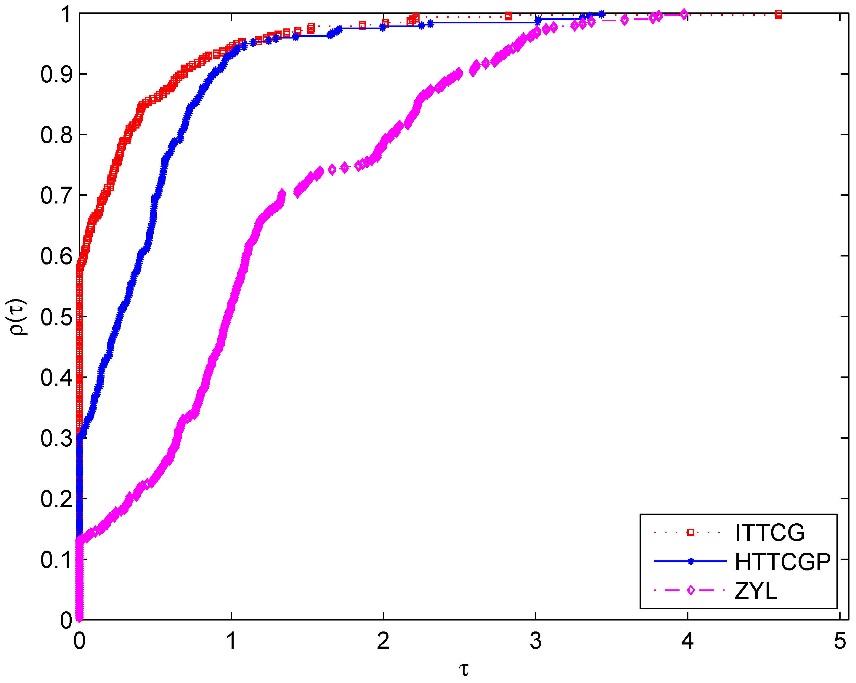
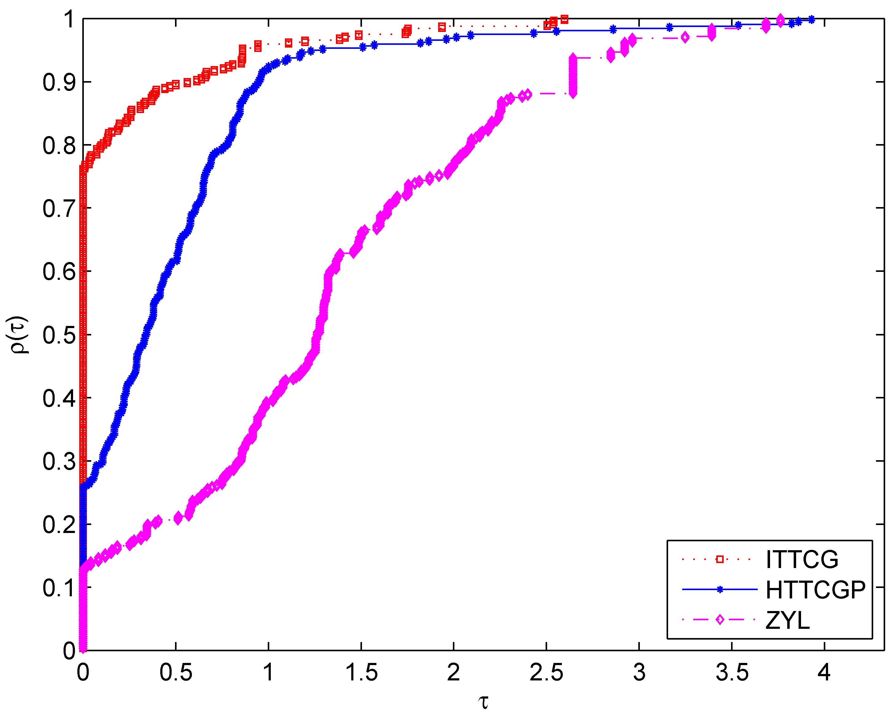
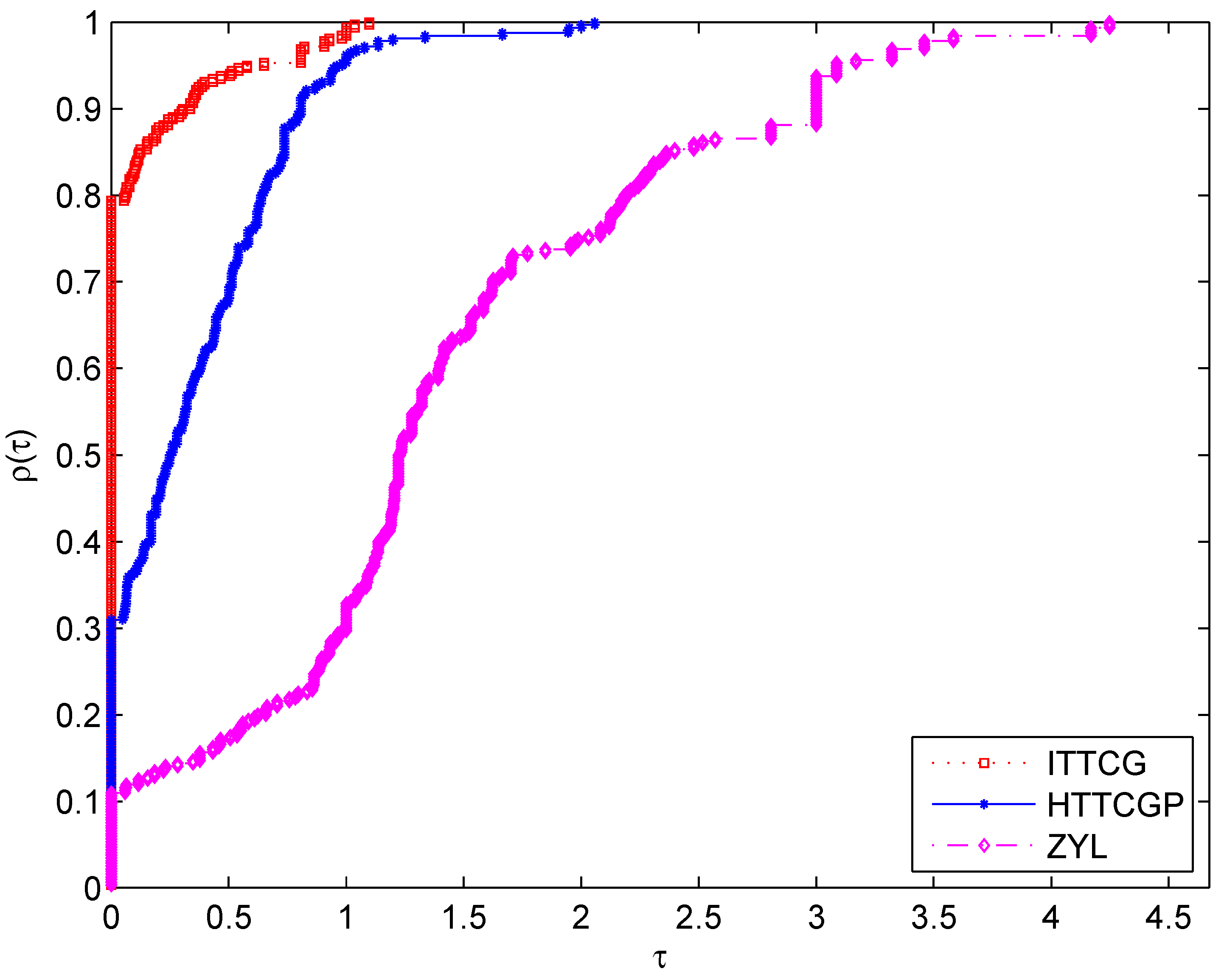
The numerical results of benchmark problems solved by Algorithms ITTCG, HTTCGP, and ZYL are presented in Table 1, Table 2, Table 3, Table 4, Table 5, Table 6, Table 7 and Table 8. In these tables, “Init(n)” refers to the initial points and the dimension multiplied by 1000. The detailed results are formatted as Time/Nfunc/Niter/Norm, where “Time” represents the CPU time in seconds, “Nfunc” represents the number of function evaluations, “Niter” represents the number of iterations, and “Norm” represents the norm of the function at the approximate optimal point. These tables illustrate that all three algorithms were capable of solving the benchmark problems across various initial points and dimensions. Notably, Algorithm ITTCG exhibited superior performance in most cases. To clearly demonstrate the performance of Algorithm ITTCG, we utilized the performance profiles developed by Dolan and Moré [29]. These profiles visually compared the performance in terms of CPU time, Nfunc, and Niter, as shown in Figure 1, Figure 2 and Figure 3. From these figures, we can observe that Algorithm ITTCG won about 59%, 77%, and 80% of the experiments in terms of CPU time, Nfunc, and Niter, respectively. The results indicate that Algorithm ITTCG outperformed Algorithm HTTCGP and ZYL on the given benchmark problems.

5. Applications in Image Denoising

Image denoising, a well-known inverse problem in the field of compressive sensing, poses significant challenges due to various sources of image noise. This noise can originate from faulty pixels in camera sensors, errors in hardware storage locations, or transmission through noisy channels. Some pixels in the image are contaminated by Gaussian noise, known as additive white Gaussian noise (AWGN), or impulse noise, known as salt-and-pepper noise. Our primary focus is on images affected by salt-and-pepper noise. This type of noise is particularly challenging because it can obscure important image details and edges, which are critical for various image processing applications such as medical imaging, remote sensing, and object recognition. In the works [30,31], a robust two-phase scheme was proposed to detect and remove salt-and-pepper noise. The first stage involves using an adaptive median filter to identify noisy pixels. The adaptive median filter is effective because it can handle varying noise densities and preserve image edges better than standard median filters. Once the noisy pixels have been detected, the second stage employs variational methods to restore the image. Variational methods are advantageous because they formulate image restoration as an optimization problem, balancing between data fidelity and the smoothness of the image. To enhance readability and comprehensiveness, we now provide an in-depth and concise explanation of this method.
Given an original image x with dimensions m × n , let x i , j represent the grayscale level at the pixel location ( i , j ) A = { 1 , 2 , , m } × { 1 , 2 , , n } . To facilitate image processing and analysis, we often consider the neighborhood of each pixel. Let V i , j denote the neighborhood of ( i , j ) , defined as V i , j = { ( i , j 1 ) , ( i , j + 1 ) , ( i 1 , j ) , ( i + 1 , j ) } . This represents the four direct neighbors of the pixel at ( i , j ) : left, right, up, and down. A common type of noise is salt-and-pepper noise, which randomly alters the pixel values to either the minimum or maximum grayscale level, creating a “salt-and-pepper” appearance. When the image x is corrupted by salt-and-pepper noise, the observed noisy image is presented by y. The grayscale level at pixel location ( i , j ) in the noisy image y is given by the following probabilistic model:
y i , j = x i , j , with probability 1 r , s m i n , with probability p , s m a x with probability q ,
where [ s m i n , s m a x ] is the range of x i , j , and r = q + p represents the overall noise level. To obtain the denoised image u * , we employ a comprehensive two-phase scheme. In the first stage, we apply an adaptive median filter to the noisy image y. This process results in an intermediate image, denoted as y ˜ . Based on the differences between the noisy image y and the filtered image y ˜ , we define the noise candidate set as follows:
N = { ( i , j ) A : y ˜ i , j y i , j and y i , j = s m i n or s m a x } .
In the second stage, we proceed with the recovery of the noisy pixels identified in the set N . For each pixel ( i , j ) N , if it is not contaminated by noise, we retain its original value, i.e., u i , j * = y i , j . For noisy pixels y i , j , ( i , j ) N , we need to perform recovery. We set u m , n * = y m , n for ( m , n ) V i , j N , ensuring that neighboring non-noisy pixels are preserved. For the pixels ( m , n ) V i , j N , which are in the neighborhood and are also candidates for noise, we must also recover their values. To restore the image, we aim to minimize the following function:
min u E ( u ) = ( i , j ) N ( m , n ) V i , j N 2 ϕ α ( u i , j y m , n ) + ( m , n ) V i , j N ϕ α ( u i , j u m , n ) ,
where ϕ α is an even edge-preserving potential function with parameter α . We know from [11] that if ϕ α is convex, then E ( u ) is monotone.
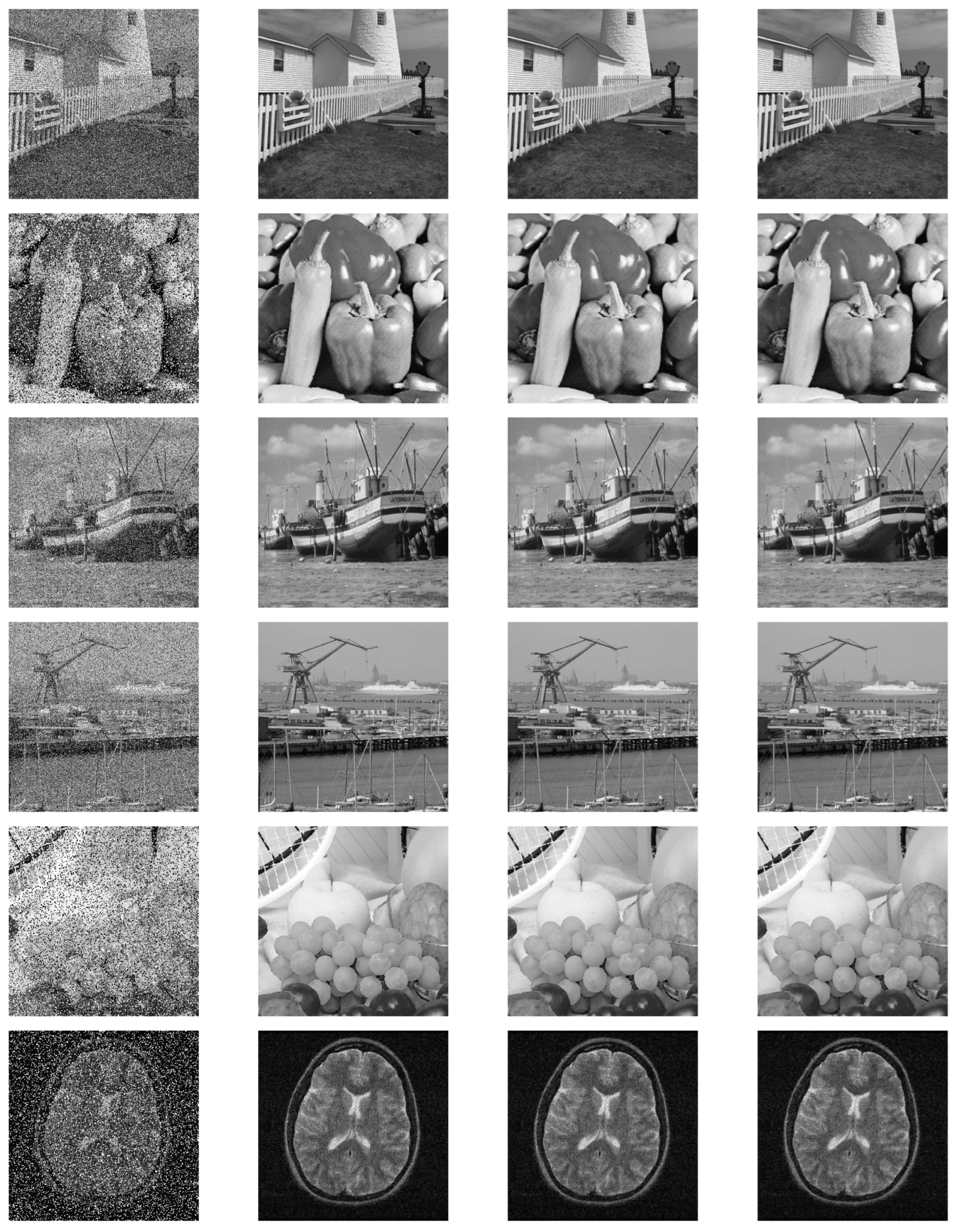
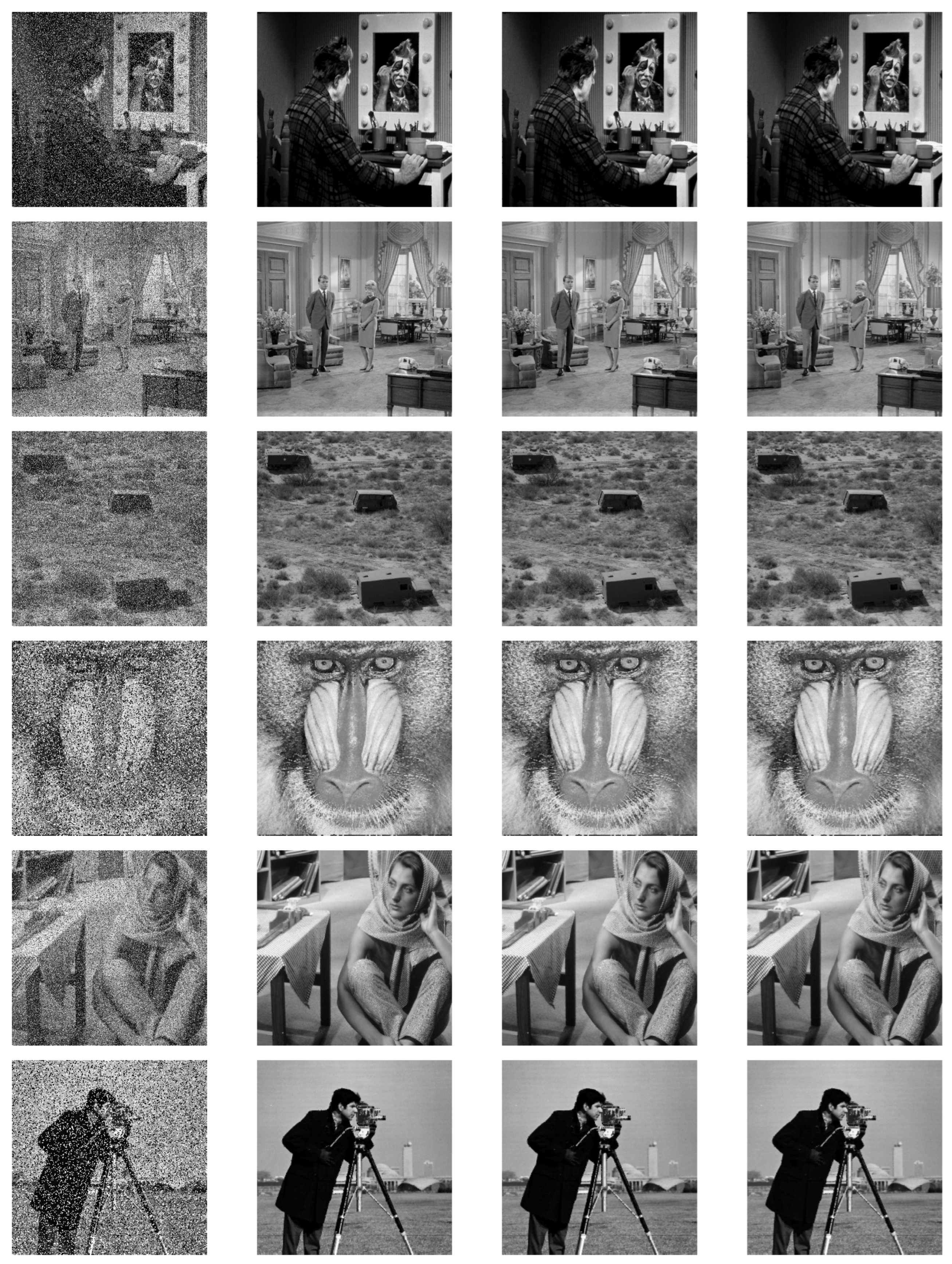
We utilized the well-known grayscale test images: lighthouse (512 × 512), peppers (256 × 256), boat (512 × 512), Kiel (512 × 512), fruits (256 × 256), brain (256 × 256), clown (512 × 512), couple (512 × 512), trucks (512 × 512), baboon (256 × 256), Barbara (512 × 512), and cameraman (256 × 256). Each image was affected by 30% salt-and-pepper noise, and the experiments were repeated 10 times with different noise samples. The detailed numerical results are presented in Table 9, where Niter ¯ , Time ¯ , PSNR ¯ , and SSIM ¯ represent the number of average iterations, the average CPU time in seconds, the average peak signal-to-noise ratio, and the average structural similarity index, respectively. Additionally, we display the noisy images with 30% salt-and-pepper noise and the images restored using the ITTCG, HTTCGP, and ZYL algorithms (see Figure 4 and Figure 5). From the results in Table 9, and Figure 4 and Figure 5, we can draw the following conclusions: (i) All images affected by 30% salt-and-pepper noise were successfully recovered by the ITTCG, HTTCGP, and ZYL algorithms. (ii) With a similar average structural similarity index, Algorithm ITTCG generally required less CPU time, fewer iterations, and achieved a lower peak signal-to-noise-ratio than the HTTCGP and ZYL algorithms, indicating that Algorithm ITTCG was efficient and competitive in image denoising.

6. Conclusions

In this paper, we proposed a projection-based improved three-term conjugate gradient algorithm for solving constrained nonlinear monotone equations. Its search direction automatically satisfies the sufficient descent and trust-region properties. The global convergence of the proposed algorithm is established under the assumption that the mapping is continuous and monotonic. A notable theoretical advantage of the proposed algorithm is that it does not require Lipschitz continuity of the mapping, unlike traditional algorithms for similar problems. Numerical results on benchmark problems demonstrated the effectiveness and competitiveness of the proposed algorithm. Furthermore, the proposed algorithm could successfully recover noise images.

Author Contributions

Conceptualization, D.L. and S.W.; Formal analysis, Y.L.; Funding acquisition, Y.L. and S.W.; Methodology, D.L.; Resources, Y.L.; Software, D.L.; Validation, D.L., Y.L., and S.W.; Writing—original draft, D.L.; Writing—review and editing, Y.L. and S.W. All authors have read and agreed to the published version of the manuscript.

Funding

This research was funded by the National Natural Science Foundation in China (grant number 11661009), the Natural Science Foundation in Guangxi Province, PR China (grant number 2024GXNSFAA010478; 2020GXNSFAA159069), the Special projects in key areas of ordinary universities in Guangdong Province (grant number 2023ZDZX4069), and the Research Team Project of Guangzhou Huashang University (grant number 2021HSKT01).

Data Availability Statement

The original contributions presented in the study are included in the article, further inquiries can be directed to the corresponding author.

Conflicts of Interest

The authors declare no conflicts of interest.

References

  1. Garcke, H.; Hüttl, P.; Knopf, P. Shape and topology optimization involving the eigenvalues of an elastic structure: A multi-phase-field approach. Adv. Nonlinear Anal. 2021, 11, 159–197. [Google Scholar] [CrossRef]
  2. Garcke, H.; Knopf, P.; Yayla, S. Long-time dynamics of the Cahn–Hilliard equation with kinetic rate dependent dynamic boundary conditions. Nonlinear Anal. 2022, 215, 112619. [Google Scholar] [CrossRef]
  3. Liu, J.; Du, X. A gradient projection method for the sparse signal reconstruction in compressive sensing. Appl. Anal. 2018, 97, 2122–2131. [Google Scholar] [CrossRef]
  4. Xiao, Y.; Zhu, H. A conjugate gradient method to solve convex constrained monotone equations with applications in compressive sensing. J. Math. Anal. Appl. 2013, 405, 310–319. [Google Scholar] [CrossRef]
  5. Dirkse, S.; Ferris, M. MCPLIB: A collection of nonlinear mixed complementarity problems. Optim. Methods Softw. 1995, 5, 319–345. [Google Scholar] [CrossRef]
  6. Wood, A.; Wollenberg, B. Power Generation, Operation, and Control; Wiley: New York, NY, USA, 1996. [Google Scholar]
  7. Li, D.; Wang, S.; Li, Y.; Wu, J. A convergence analysis of hybrid gradient projection algorithm for constrained nonlinear equations with applications in compressed sensing. Numer. Algorithms 2024, 95, 1325–1345. [Google Scholar] [CrossRef]
  8. Li, D.; Wu, J.; Li, Y.; Wang, S. A modified spectral gradient projection-based algorithm for large-scale constrained nonlinear equations with applications in compressive sensing. J. Comput. Appl. Math. 2023, 424, 115006. [Google Scholar] [CrossRef]
  9. Liu, J.; Duan, Y. Two spectral gradient projection methods for constrained equations and their linear convergence rate. J. Inequal. Appl. 2015, 2015, 8. [Google Scholar] [CrossRef]
  10. Sulaiman, I.M.; Awwal, A.M.; Malik, M. A derivative-free mzprp projection method for convex constrained nonlinear equations and its application in compressive sensing. Mathematics 2022, 10, 2884. [Google Scholar] [CrossRef]
  11. Li, D.; Wang, S.; Li, Y.; Wu, J. A projection-based hybrid PRP-DY type conjugate gradient algorithm for constrained nonlinear equations with applications. Appl. Numer. Math. 2024, 195, 105–125. [Google Scholar] [CrossRef]
  12. Yin, J.; Jian, J.; Jiang, X. A generalized hybrid CGPM-based algorithm for solving large-scale convex constrained equations with applications to image restoration. J. Comput. Appl. Math. 2021, 391, 113423. [Google Scholar] [CrossRef]
  13. Liu, P.; Jian, J.; Jiang, X. A new conjugate gradient projection method for convex constrained nonlinear equations. Complexity 2020, 2020, 8323865. [Google Scholar] [CrossRef]
  14. Yuan, G.; Li, T.; Hu, W. A conjugate gradient algorithm for large-scale nonlinear equations and image restoration problems. Appl. Numer. Math. 2020, 147, 129–141. [Google Scholar] [CrossRef]
  15. Ali, E.; Mahdi, S. Adaptive hybrid mixed two-point step size gradient algorithm for solving non-linear systems. Mathematics 2023, 11, 2102. [Google Scholar] [CrossRef]
  16. Kumam, P.; Abubakar, A.B.; Malik, M. A hybrid HS-LS conjugate gradient algorithm for unconstrained optimization with applications in motion control and image recovery. J. Comput. Appl. Math. 2023, 433, 115304. [Google Scholar] [CrossRef]
  17. Ullah, N.; Shah, A.; Sabíu, J. A one-parameter memoryless DFP algorithm for solving system of monotone nonlinear equations with application in image processing. Mathematics 2023, 11, 1221. [Google Scholar] [CrossRef]
  18. Yin, J.; Jian, J.; Jiang, X. A hybrid three-term conjugate gradient projection method for constrained nonlinear monotone equations with applications. Numer. Algorithms 2021, 88, 389–418. [Google Scholar] [CrossRef]
  19. Gao, P.; He, C. An efficient three-term conjugate gradient method for nonlinear monotone equations with convex constraints. Calcolo 2018, 55, 53. [Google Scholar] [CrossRef]
  20. Yuan, G.; Zhang, M. A three-terms Polak–Ribière–Polyak conjugate gradient algorithm for large-scale nonlinear equations. J. Comput. Appl. Math. 2015, 286, 186–195. [Google Scholar] [CrossRef]
  21. Jiang, X.; Liao, W.; Yin, J. A new family of hybrid three-term conjugate gradient methods with applications in image restoration. Numer. Algorithms 2022, 91, 161–191. [Google Scholar] [CrossRef]
  22. Liu, Y.; Zhu, Z.; Zhang, B. Two sufficient descent three-term conjugate gradient methods for unconstrained optimization problems with applications in compressive sensing. J. Appl. Math. Comput. 2022, 1–30. [Google Scholar] [CrossRef]
  23. Kim, H.; Wang, C.; Byun, H. Variable three-term conjugate gradient method for training artificial neural networks. Neural Networks 2023, 159, 125–136. [Google Scholar] [CrossRef]
  24. Li, M. A modified Hestense-Stiefel conjugate gradient method close to the memoryless BFGS quasi-Newton method. Optim. Methods Softw. 2018, 33, 336–353. [Google Scholar] [CrossRef]
  25. Li, M. A three-term polak-ribière-polyak conjugate gradient method close to the memoryless BFGS quasi-Newton mthod. J. Ind. Manag. Optim. 2017, 13, 1–16. [Google Scholar]
  26. Li, M. A family of three-term nonlinear conjugate gradient methods close to the memoryless BFGS method. Optim. Lett. 2018, 12, 1911–1927. [Google Scholar] [CrossRef]
  27. Ding, Y.; Xiao, Y.; Li, J. A class of conjugate gradient methods for convex constrained monotone equations. Optimization 2017, 66, 2309–2328. [Google Scholar] [CrossRef]
  28. Zheng, L.; Yang, L.; Liang, Y. A conjugate gradient projection method for solving equations with convex constraints. J. Comput. Appl. Math. 2020, 375, 112781. [Google Scholar] [CrossRef]
  29. Dolan, E.; Moré, J. Benchmarking optimization software with performance profiles. Math. Program. 2002, 91, 201–213. [Google Scholar] [CrossRef]
  30. Chan, R.; Ho, C.; Nikolova, M. Salt-and-pepper noise removal by median-type noise detectors and detail-preserving regularization. IEEE Trans. Image Process. 2005, 14, 1479–1485. [Google Scholar] [CrossRef]
  31. Cai, J.; Chan, R.; Fiore, D. Minimization of a detail-preserving regularization functional for impulse noise removal. J. Math. Imaging Vis. 2007, 29, 79–91. [Google Scholar] [CrossRef]
Figure 1. Performance profiles for time.
Mathematics 12 02556 g001
Figure 2. Performance profiles for Nfunc.
Mathematics 12 02556 g002
Figure 3. Performance profiles for Niter.
Mathematics 12 02556 g003
Figure 4. The noise images for lighthouse, peppers, boat, Kiel, fruits, and brain with 30% salt and pepper noise (first column) and the images recovered by Algorithms ITTCG (second column), HTTCGP (third column), and ZYL (forth column).
Mathematics 12 02556 g004
Figure 5. The noise images for clown, couple, trucks, baboon, Barbara, and cameraman with 30% salt and pepper noise (first column) and the images recovered by Algorithms ITTCG (second column), HTTCGP (third column), and ZYL (forth column).
Mathematics 12 02556 g005
Table 1. Numerical results for Problem 1.
Init (n)ITTCGHTTCGPZYL
Time/Nfunc/Niter/NormTime/Nfunc/Niter/NormTime/Nfunc/Niter/Norm
x1(1)8.30 × 10 3 /7/1/0.00 × 10 0 2.89 × 10 3 /7/1/0.00 × 10 0 3.77 × 10 3 /90/18/9.93 × 10 7
x2(1)7.84 × 10 4 /4/1/0.00 × 10 0 1.11 × 10 4 /4/1/0.00 × 10 0 5.27 × 10 4 /25/8/1.84 × 10 7
x3(1)1.53 × 10 3 /78/16/5.89 × 10 7 1.56 × 10 3 /84/17/4.60 × 10 7 4.51 × 10 3 /261/62/6.28 × 10 7
x4(1)1.16 × 10 3 /53/11/3.86 × 10 7 1.44 × 10 3 /69/15/2.46 × 10 7 1.84 × 10 3 /100/20/5.05 × 10 7
x5(1)1.93 × 10 3 /69/14/6.42 × 10 7 8.06 × 10 4 /38/8/6.62 × 10 7 6.76 × 10 3 /288/68/8.66 × 10 7
x6(1)1.49 × 10 3 /53/11/3.94 × 10 7 1.52 × 10 3 /69/15/3.14 × 10 7 2.03 × 10 3 /100/20/5.09 × 10 7
x7(1)1.35 × 10 3 /53/11/3.44 × 10 7 1.78 × 10 3 /69/15/1.28 × 10 7 2.96 × 10 3 /100/20/5.60 × 10 7
x8(1)1.28 × 10 3 /53/11/8.69 × 10 7 2.57 × 10 3 /108/21/9.53 × 10 7 1.95 × 10 3 /100/20/4.68 × 10 7
x1(5)1.35 × 10 3 /7/1/0.00 × 10 0 8.77 × 10 4 /7/1/0.00 × 10 0 1.23 × 10 2 /90/18/8.21 × 10 7
x2(5)5.94 × 10 4 /4/1/0.00 × 10 0 5.96 × 10 4 /4/1/0.00 × 10 0 4.38 × 10 3 /25/8/1.84 × 10 7
x3(5)6.18 × 10 4 /4/1/0.00 × 10 0 4.95 × 10 4 /4/1/0.00 × 10 0 3.91 × 10 3 /25/8/2.00 × 10 7
x4(5)5.79 × 10 3 /44/9/3.64 × 10 7 8.06 × 10 3 /69/15/2.23 × 10 7 1.18 × 10 2 /105/21/4.48 × 10 7
x5(5)8.99 × 10 3 /69/14/6.60 × 10 7 5.43 × 10 3 /38/8/6.39 × 10 7 3.46 × 10 2 /288/68/8.67 × 10 7
x6(5)5.24 × 10 3 /44/9/3.72 × 10 7 8.65 × 10 3 /69/15/4.01 × 10 7 1.04 × 10 2 /105/21/4.49 × 10 7
x7(5)5.48 × 10 3 /44/9/3.98 × 10 7 7.85 × 10 3 /69/15/3.15 × 10 7 1.16 × 10 2 /105/21/4.60 × 10 7
x8(5)6.42 × 10 3 /53/11/5.88 × 10 7 8.85 × 10 3 /69/15/9.92 × 10 9 1.16 × 10 2 /105/21/4.40 × 10 7
x1(10)1.28 × 10 3 /7/1/0.00 × 10 0 1.25 × 10 3 /7/1/0.00 × 10 0 1.50 × 10 2 /90/18/8.80 × 10 7
x2(10)8.37 × 10 4 /4/1/0.00 × 10 0 7.26 × 10 4 /4/1/0.00 × 10 0 5.07 × 10 3 /25/8/1.84 × 10 7
x3(10)7.53 × 10 4 /4/1/0.00 × 10 0 7.21 × 10 4 /4/1/0.00 × 10 0 5.80 × 10 3 /25/8/2.00 × 10 7
x4(10)8.52 × 10 3 /44/9/1.54 × 10 7 1.28 × 10 2 /69/15/3.77 × 10 7 1.82 × 10 2 /105/21/6.34 × 10 7
x5(10)1.33 × 10 2 /69/14/6.62 × 10 7 6.92 × 10 3 /38/8/6.36 × 10 7 5.57 × 10 2 /288/68/8.67 × 10 7
x6(10)9.67 × 10 3 /44/9/1.58 × 10 7 1.39 × 10 2 /69/15/5.06 × 10 7 1.91 × 10 2 /105/21/6.34 × 10 7
x7(10)9.01 × 10 3 /44/9/1.69 × 10 7 1.37 × 10 2 /69/15/4.45 × 10 7 1.92 × 10 2 /105/21/6.42 × 10 7
x8(10)1.15 × 10 2 /53/11/2.05 × 10 8 1.39 × 10 2 /69/15/2.94 × 10 8 1.83 × 10 2 /105/21/6.17 × 10 7
x1(50)5.84 × 10 3 /7/1/0.00 × 10 0 3.71 × 10 3 /7/1/0.00 × 10 0 5.84 × 10 2 /95/19/5.74 × 10 7
x2(50)2.75 × 10 3 /4/1/0.00 × 10 0 2.56 × 10 3 /4/1/0.00 × 10 0 1.56 × 10 2 /25/8/1.84 × 10 7
x3(50)2.46 × 10 3 /4/1/0.00 × 10 0 2.31 × 10 3 /4/1/0.00 × 10 0 1.60 × 10 2 /25/8/2.00 × 10 7
x4(50)5.49 × 10 2 /81/17/5.07 × 10 7 4.94 × 10 2 /69/15/9.57 × 10 7 6.51 × 10 2 /110/22/5.60 × 10 7
x5(50)4.53 × 10 2 /69/14/6.64 × 10 7 2.60 × 10 2 /38/8/6.34 × 10 7 1.84 × 10 1 /288/68/8.67 × 10 7
x6(50)5.33 × 10 2 /76/16/8.44 × 10 7 5.10 × 10 2 /74/16/6.93 × 10 8 6.71 × 10 2 /110/22/5.60 × 10 7
x7(50)5.21 × 10 2 /76/16/4.33 × 10 7 4.64 × 10 2 /69/15/9.88 × 10 7 6.74 × 10 2 /110/22/5.62 × 10 7
x8(50)3.59 × 10 2 /48/10/0.00 × 10 0 5.82 × 10 2 /78/17/7.67 × 10 7 6.84 × 10 2 /110/22/5.55 × 10 7
x1(100)9.61 × 10 3 /7/1/0.00 × 10 0 9.45 × 10 3 /7/1/0.00 × 10 0 1.29 × 10 1 /95/19/7.76 × 10 7
x2(100)6.76 × 10 3 /4/1/0.00 × 10 0 5.55 × 10 3 /4/1/0.00 × 10 0 3.12 × 10 2 /25/8/1.84 × 10 7
x3(100)5.52 × 10 3 /4/1/0.00 × 10 0 5.36 × 10 3 /4/1/0.00 × 10 0 3.02 × 10 2 /25/8/2.00 × 10 7
x4(100)7.97 × 10 2 /52/11/0.00 × 10 0 1.12 × 10 1 /74/16/6.18 × 10 8 1.42 × 10 1 /110/22/7.92 × 10 7
x5(100)9.69 × 10 2 /69/14/6.64 × 10 7 5.44 × 10 2 /38/8/6.33 × 10 7 3.61 × 10 1 /288/68/8.67 × 10 7
x6(100)7.86 × 10 2 /52/11/0.00 × 10 0 1.10 × 10 1 /74/16/8.59 × 10 8 1.40 × 10 1 /110/22/7.92 × 10 7
x7(100)8.00 × 10 2 /52/11/0.00 × 10 0 1.15 × 10 1 /74/16/7.44 × 10 8 1.82 × 10 1 /110/22/7.94 × 10 7
x8(100)1.02 × 10 1 /62/13/5.59 × 10 7 1.25 × 10 1 /78/17/9.11 × 10 7 1.43 × 10 1 /110/22/7.88 × 10 7
Table 2. Numerical results for Problem 2.
Init(n)ITTCGHTTCGPZYL
Time/Nfunc/Niter/NormTime/Nfunc/Niter/NormTime/Nfunc/Niter/Norm
x1(1)3.05 × 10 3 /5/1/0.00 × 10 0 1.26 × 10 4 /5/1/0.00 × 10 0 6.58 × 10 4 /36/11/1.82 × 10 7
x2(1)9.14 × 10 5 /4/1/0.00 × 10 0 1.24 × 10 4 /4/1/0.00 × 10 0 4.13 × 10 4 /25/8/1.84 × 10 7
x3(1)4.95 × 10 4 /22/8/9.13 × 10 7 4.36 × 10 4 /23/8/1.61 × 10 7 1.46 × 10 3 /94/31/5.23 × 10 7
x4(1)1.06 × 10 3 /47/15/2.08 × 10 7 1.23 × 10 3 /59/19/9.26 × 10 7 2.11 × 10 3 /117/38/7.52 × 10 7
x5(1)5.70 × 10 4 /24/8/6.49 × 10 8 5.69 × 10 4 /28/9/6.46 × 10 8 1.43 × 10 3 /81/26/9.56 × 10 7
x6(1)9.49 × 10 4 /40/13/5.57 × 10 7 7.91 × 10 4 /38/13/8.06 × 10 9 2.14 × 10 3 /121/39/4.72 × 10 7
x7(1)1.06 × 10 3 /47/15/2.08 × 10 7 1.15 × 10 3 /59/19/9.26 × 10 7 2.06 × 10 3 /117/38/7.52 × 10 7
x8(1)1.03 × 10 3 /39/14/1.88 × 10 7 9.06 × 10 4 /40/13/4.75 × 10 7 1.42 × 10 3 /76/24/8.46 × 10 7
x1(5)5.79 × 10 4 /5/1/0.00 × 10 0 4.40 × 10 4 /5/1/0.00 × 10 0 4.36 × 10 3 /36/11/4.07 × 10 7
x2(5)3.91 × 10 4 /4/1/0.00 × 10 0 4.16 × 10 4 /4/1/0.00 × 10 0 2.82 × 10 3 /25/8/1.84 × 10 7
x3(5)5.10 × 10 4 /4/1/0.00 × 10 0 4.63 × 10 4 /4/1/0.00 × 10 0 3.11 × 10 3 /25/8/2.00 × 10 7
x4(5)6.11 × 10 3 /45/15/3.16 × 10 7 6.60 × 10 3 /55/18/1.08 × 10 12 1.27 × 10 2 /126/41/8.02 × 10 7
x5(5)2.69 × 10 3 /24/8/9.08 × 10 8 2.99 × 10 3 /28/9/8.18 × 10 8 8.06 × 10 3 /81/26/9.57 × 10 7
x6(5)4.58 × 10 3 /44/14/5.94 × 10 7 4.47 × 10 3 /43/15/6.72 × 10 8 1.00 × 10 2 /106/34/9.43 × 10 7
x7(5)4.87 × 10 3 /45/15/3.16 × 10 7 6.44 × 10 3 /55/18/1.08 × 10 12 1.11 × 10 2 /126/41/8.02 × 10 7
x8(5)6.10 × 10 3 /50/17/7.67 × 10 8 4.00 × 10 3 /38/13/7.39 × 10 7 1.15 × 10 2 /123/40/6.51 × 10 7
x1(10)6.70 × 10 4 /5/1/0.00 × 10 0 6.54 × 10 4 /5/1/0.00 × 10 0 4.92 × 10 3 /36/11/5.75 × 10 7
x2(10)5.04 × 10 4 /4/1/0.00 × 10 0 5.16 × 10 4 /4/1/0.00 × 10 0 3.03 × 10 3 /25/8/1.84 × 10 7
x3(10)5.41 × 10 4 /4/1/0.00 × 10 0 6.07 × 10 4 /4/1/0.00 × 10 0 3.99 × 10 3 /25/8/2.00 × 10 7
x4(10)9.40 × 10 3 /52/16/7.66 × 10 7 8.07 × 10 3 /56/18/5.41 × 10 10 1.80 × 10 2 /129/42/6.00 × 10 7
x5(10)4.74 × 10 3 /24/8/9.43 × 10 8 4.19 × 10 3 /28/9/8.42 × 10 8 1.18 × 10 2 /81/26/9.57 × 10 7
x6(10)8.57 × 10 3 /51/16/8.19 × 10 7 8.58 × 10 3 /58/19/2.93 × 10 7 1.59 × 10 2 /112/36/4.86 × 10 7
x7(10)1.06 × 10 2 /52/16/7.66 × 10 7 9.62 × 10 3 /56/18/5.41 × 10 10 1.94 × 10 2 /129/42/6.00 × 10 7
x8(10)1.30 × 10 2 /50/17/5.50 × 10 7 9.49 × 10 3 /58/19/1.09 × 10 7 2.12 × 10 2 /120/39/8.17 × 10 7
x1(50)3.13 × 10 3 /5/1/0.00 × 10 0 1.94 × 10 3 /5/1/0.00 × 10 0 2.00 × 10 2 /39/12/2.06 × 10 7
x2(50)1.69 × 10 3 /4/1/0.00 × 10 0 1.39 × 10 3 /4/1/0.00 × 10 0 1.03 × 10 2 /25/8/1.84 × 10 7
x3(50)1.71 × 10 3 /4/1/0.00 × 10 0 1.64 × 10 3 /4/1/0.00 × 10 0 1.12 × 10 2 /25/8/2.00 × 10 7
x4(50)3.51 × 10 2 /60/19/4.83 × 10 7 3.23 × 10 2 /57/18/4.68 × 10 14 6.65 × 10 2 /129/42/9.70 × 10 7
x5(50)1.48 × 10 2 /24/8/9.72 × 10 8 1.68 × 10 2 /28/9/8.62 × 10 8 4.04 × 10 2 /81/26/9.57 × 10 7
x6(50)3.64 × 10 2 /54/18/1.53 × 10 7 2.29 × 10 2 /39/14/3.40 × 10 7 5.72 × 10 2 /117/38/5.84 × 10 7
x7(50)3.77 × 10 2 /60/19/4.83 × 10 7 3.44 × 10 2 /57/18/4.68 × 10 14 6.29 × 10 2 /129/42/9.70 × 10 7
x8(50)3.82 × 10 2 /58/18/2.83 × 10 7 2.89 × 10 2 /41/14/4.10 × 10 7 6.26 × 10 2 /129/42/8.15 × 10 7
x1(100)4.75 × 10 3 /5/1/0.00 × 10 0 3.72 × 10 3 /5/1/0.00 × 10 0 3.23 × 10 2 /39/12/2.91 × 10 7
x2(100)3.49 × 10 3 /4/1/0.00 × 10 0 2.62 × 10 3 /4/1/0.00 × 10 0 1.60 × 10 2 /25/8/1.84 × 10 7
x3(100)3.94 × 10 3 /4/1/0.00 × 10 0 3.03 × 10 3 /4/1/0.00 × 10 0 1.60 × 10 2 /25/8/2.00 × 10 7
x4(100)4.69 × 10 2 /41/15/3.94 × 10 8 3.74 × 10 2 /41/14/3.81 × 10 7 1.06 × 10 1 /132/43/8.32 × 10 7
x5(100)2.63 × 10 2 /24/8/9.75 × 10 8 2.77 × 10 2 /28/9/8.64 × 10 8 6.34 × 10 2 /81/26/9.57 × 10 7
x6(100)5.50 × 10 2 /47/18/3.93 × 10 7 4.14 × 10 2 /43/15/4.35 × 10 8 1.04 × 10 1 /129/42/5.76 × 10 7
x7(100)4.78 × 10 2 /41/15/3.94 × 10 8 4.06 × 10 2 /41/14/3.81 × 10 7 1.10 × 10 1 /132/43/8.32 × 10 7
x8(100)6.30 × 10 2 /48/17/3.01 × 10 7 5.47 × 10 2 /45/16/4.28 × 10 15 1.07 × 10 1 /129/42/7.87 × 10 7
Table 3. Numerical results for Problem 3.
Init(n)ITTCGHTTCGPZYL
Time/Nfunc/Niter/NormTime/Nfunc/Niter/NormTime/Nfunc/Niter/Norm
x1(1)5.36 × 10 3 /250/33/5.87 × 10 7 5.72 × 10 3 /293/36/9.74 × 10 7 8.26 × 10 3 /439/73/9.64 × 10 7
x2(1)3.93 × 10 3 /180/23/7.99 × 10 7 5.81 × 10 3 /307/38/8.37 × 10 7 7.07 × 10 3 /367/61/9.94 × 10 7
x3(1)4.19 × 10 3 /208/27/8.37 × 10 7 6.63 × 10 3 /349/43/8.55 × 10 7 7.49 × 10 3 /385/64/8.74 × 10 7
x4(1)4.51 × 10 3 /222/29/6.50 × 10 7 8.57 × 10 3 /433/54/9.46 × 10 7 7.66 × 10 3 /391/65/9.70 × 10 7
x5(1)4.73 × 10 3 /237/31/6.04 × 10 7 6.64 × 10 3 /337/42/8.37 × 10 7 7.42 × 10 3 /391/65/9.80 × 10 7
x6(1)4.61 × 10 3 /222/29/6.49 × 10 7 8.58 × 10 3 /410/51/9.15 × 10 7 8.01 × 10 3 /397/66/9.25 × 10 7
x7(1)5.08 × 10 3 /250/33/5.41 × 10 7 6.35 × 10 3 /330/41/8.54 × 10 7 7.97 × 10 3 /421/70/9.17 × 10 7
x8(1)6.45 × 10 3 /308/41/5.09 × 10 7 8.47 × 10 3 /413/51/9.89 × 10 7 9.79 × 10 3 /480/80/9.21 × 10 7
x1(5)3.76 × 10 2 /243/32/6.03 × 10 7 3.64 × 10 2 /299/37/8.62 × 10 7 5.50 × 10 2 /445/74/8.19 × 10 7
x2(5)2.20 × 10 2 /173/22/8.68 × 10 7 3.98 × 10 2 /338/42/1.00 × 10 6 4.94 × 10 2 /403/67/9.85 × 10 7
x3(5)2.43 × 10 2 /201/26/8.32 × 10 7 3.75 × 10 2 /319/39/9.75 × 10 7 4.98 × 10 2 /415/69/9.21 × 10 7
x4(5)2.67 × 10 2 /229/30/8.15 × 10 7 4.77 × 10 2 /418/52/3.03 × 10 7 5.21 × 10 2 /421/70/7.23 × 10 7
x5(5)2.62 × 10 2 /216/28/5.92 × 10 7 3.86 × 10 2 /316/39/7.17 × 10 7 5.17 × 10 2 /415/69/8.21 × 10 7
x6(5)2.92 × 10 2 /229/30/8.14 × 10 7 5.12 × 10 2 /417/52/9.34 × 10 7 5.52 × 10 2 /415/69/8.50 × 10 7
x7(5)3.48 × 10 2 /271/36/7.63 × 10 7 7.09 × 10 2 /560/70/9.12 × 10 7 5.42 × 10 2 /439/73/7.95 × 10 7
x8(5)4.21 × 10 2 /309/41/5.34 × 10 7 5.09 × 10 2 /413/51/5.52 × 10 7 6.69 × 10 2 /522/87/9.37 × 10 7
x1(10)4.56 × 10 2 /236/31/6.73 × 10 7 6.37 × 10 2 /338/42/3.92 × 10 7 8.78 × 10 2 /451/75/9.13 × 10 7
x2(10)3.39 × 10 2 /187/24/9.18 × 10 7 6.63 × 10 2 /338/42/9.20 × 10 7 7.80 × 10 2 /415/69/9.61 × 10 7
x3(10)3.83 × 10 2 /208/27/9.16 × 10 7 6.19 × 10 2 /335/42/6.78 × 10 7 7.91 × 10 2 /427/71/9.89 × 10 7
x4(10)4.54 × 10 2 /236/31/7.88 × 10 7 6.21 × 10 2 /359/45/4.72 × 10 7 6.89 × 10 2 /397/66/6.98 × 10 7
x5(10)4.12 × 10 2 /223/29/5.94 × 10 7 5.37 × 10 2 /302/37/5.30 × 10 7 7.13 × 10 2 /409/68/9.04 × 10 7
x6(10)4.33 × 10 2 /236/31/7.88 × 10 7 6.24 × 10 2 /369/46/3.53 × 10 7 6.95 × 10 2 /397/66/7.00 × 10 7
x7(10)5.05 × 10 2 /264/35/8.21 × 10 7 9.77 × 10 2 /568/71/5.46 × 10 7 7.02 × 10 2 /397/66/9.17 × 10 7
x8(10)5.65 × 10 2 /309/41/7.30 × 10 7 6.72 × 10 2 /387/48/8.03 × 10 7 8.77 × 10 2 /486/81/7.25 × 10 7
x1(50)1.75 × 10 1 /236/31/7.21 × 10 7 2.01 × 10 1 /292/36/6.60 × 10 7 3.00 × 10 1 /427/71/9.67 × 10 7
x2(50)1.31 × 10 1 /180/23/9.41 × 10 7 2.50 × 10 1 /350/44/9.18 × 10 7 2.97 × 10 1 /427/71/9.94 × 10 7
x3(50)1.44 × 10 1 /209/27/4.76 × 10 7 2.80 × 10 1 /412/52/8.85 × 10 7 3.02 × 10 1 /415/69/7.96 × 10 7
x4(50)1.60 × 10 1 /229/30/8.95 × 10 7 2.65 × 10 1 /394/50/8.74 × 10 7 2.90 × 10 1 /416/69/9.13 × 10 7
x5(50)1.62 × 10 1 /237/31/6.63 × 10 7 1.95 × 10 1 /288/36/9.73 × 10 7 3.12 × 10 1 /439/73/8.44 × 10 7
x6(50)1.52 × 10 1 /229/30/8.95 × 10 7 2.64 × 10 1 /387/49/8.40 × 10 7 2.90 × 10 1 /416/69/9.17 × 10 7
x7(50)1.80 × 10 1 /264/35/8.82 × 10 7 2.63 × 10 1 /381/48/7.31 × 10 7 2.79 × 10 1 /410/68/9.11 × 10 7
x8(50)2.24 × 10 1 /324/43/6.03 × 10 7 3.16 × 10 1 /451/56/7.36 × 10 7 3.41 × 10 1 /481/80/9.57 × 10 7
x1(100)4.19 × 10 1 /222/29/8.67 × 10 7 5.07 × 10 1 /261/32/7.78 × 10 7 8.75 × 10 1 /433/72/8.25 × 10 7
x2(100)3.24 × 10 1 /180/23/9.00 × 10 7 5.38 × 10 1 /265/33/7.48 × 10 7 8.16 × 10 1 /415/69/8.73 × 10 7
x3(100)3.84 × 10 1 /216/28/4.70 × 10 7 6.33 × 10 1 /320/40/4.66 × 10 7 7.70 × 10 1 /415/69/9.78 × 10 7
x4(100)4.77 × 10 1 /243/32/9.84 × 10 7 5.49 × 10 1 /378/48/8.73 × 10 7 7.55 × 10 1 /416/69/7.31 × 10 7
x5(100)4.32 × 10 1 /230/30/7.85 × 10 7 6.88 × 10 1 /344/43/9.43 × 10 7 9.14 × 10 1 /451/75/9.94 × 10 7
x6(100)4.56 × 10 1 /243/32/9.84 × 10 7 6.98 × 10 1 /347/44/9.61 × 10 7 8.11 × 10 1 /416/69/7.31 × 10 7
x7(100)4.67 × 10 1 /244/32/5.07 × 10 7 6.55 × 10 1 /317/40/6.90 × 10 7 8.56 × 10 1 /422/70/9.36 × 10 7
x8(100)6.35 × 10 1 /345/46/8.22 × 10 7 9.66 × 10 1 /475/59/7.73 × 10 7 9.91 × 10 1 /493/82/8.45 × 10 7
Table 4. Numerical results for Problem 4.
Init(n)ITTCGHTTCGPZYL
Time/Nfunc/Niter/NormTime/Nfunc/Niter/NormTime/Nfunc/Niter/Norm
x1(1)2.21 × 10 3 /89/20/2.89 × 10 7 2.83 × 10 3 /119/27/8.70 × 10 8 2.78 × 10 3 /118/38/8.33 × 10 7
x2(1)1.57 × 10 3 /51/19/1.61 × 10 7 1.56 × 10 3 /56/21/9.69 × 10 7 2.28 × 10 3 /96/33/6.03 × 10 7
x3(1)1.23 × 10 3 /39/15/8.04 × 10 7 1.53 × 10 3 /54/18/3.13 × 10 7 2.20 × 10 3 /93/32/7.55 × 10 7
x4(1)4.91 × 10 3 /223/39/4.76 × 10 7 4.59 × 10 3 /237/35/7.19 × 10 7 2.80 × 10 3 /123/39/8.83 × 10 7
x5(1)9.47 × 10 4 /29/12/4.29 × 10 7 1.40 × 10 3 /52/19/6.57 × 10 8 2.37 × 10 3 /102/35/8.01 × 10 7
x6(1)4.47 × 10 3 /212/36/8.45 × 10 7 5.37 × 10 3 /279/43/1.69 × 10 7 2.77 × 10 3 /123/39/8.74 × 10 7
x7(1)1.12 × 10 3 /37/14/1.06 × 10 7 1.41 × 10 3 /53/19/8.14 × 10 7 2.05 × 10 3 /87/30/7.34 × 10 7
x8(1)6.41 × 10 3 /328/44/6.49 × 10 7 6.04 × 10 3 /320/44/7.16 × 10 7 4.16 × 10 3 /207/50/6.30 × 10 7
x1(5)2.23 × 10 2 /231/36/1.93 × 10 7 1.77 × 10 2 /216/33/5.67 × 10 7 1.50 × 10 2 /132/42/7.97 × 10 7
x2(5)5.03 × 10 3 /39/16/7.13 × 10 7 6.34 × 10 3 /50/18/4.49 × 10 7 1.02 × 10 2 /102/35/6.85 × 10 7
x3(5)5.63 × 10 3 /39/16/8.49 × 10 7 7.93 × 10 3 /68/26/5.31 × 10 7 1.03 × 10 2 /96/33/6.96 × 10 7
x4(5)3.01 × 10 2 /373/49/6.04 × 10 7 4.30 × 10 2 /567/65/2.84 × 10 7 1.33 × 10 2 /133/42/8.46 × 10 7
x5(5)4.56 × 10 3 /36/14/2.40 × 10 7 7.41 × 10 3 /62/23/9.87 × 10 7 9.95 × 10 3 /99/34/6.30 × 10 7
x6(5)3.07 × 10 2 /376/50/1.06 × 10 7 4.29 × 10 2 /570/62/1.23 × 10 7 1.31 × 10 2 /141/45/7.46 × 10 7
x7(5)6.42 × 10 3 /45/17/3.98 × 10 7 6.82 × 10 3 /61/22/7.17 × 10 7 1.05 × 10 2 /96/33/5.87 × 10 7
x8(5)4.89 × 10 2 /637/69/9.82 × 10 7 4.17 × 10 2 /562/63/6.41 × 10 8 1.70 × 10 2 /189/44/9.43 × 10 7
x1(10)2.08 × 10 2 /93/24/3.59 × 10 7 3.40 × 10 2 /265/34/3.37 × 10 7 2.11 × 10 2 /118/38/7.24 × 10 7
x2(10)1.13 × 10 2 /42/16/1.55 × 10 7 6.60 × 10 3 /35/13/3.54 × 10 7 2.09 × 10 2 /108/37/5.11 × 10 7
x3(10)1.12 × 10 2 /45/17/3.65 × 10 7 1.33 × 10 2 /55/20/9.85 × 10 7 1.98 × 10 2 /108/37/5.70 × 10 7
x4(10)6.45 × 10 2 /464/57/8.15 × 10 8 1.00 × 10 1 /811/87/5.54 × 10 7 2.51 × 10 2 /138/44/7.43 × 10 7
x5(10)1.15 × 10 2 /37/15/9.00 × 10 7 9.85 × 10 3 /51/19/2.68 × 10 7 1.91 × 10 2 /102/35/5.79 × 10 7
x6(10)6.39 × 10 2 /461/56/9.13 × 10 7 1.17 × 10 1 /1002/101/2.35 × 10 7 2.36 × 10 2 /138/44/9.78 × 10 7
x7(10)1.23 × 10 2 /43/17/4.03 × 10 7 1.32 × 10 2 /53/21/7.96 × 10 7 2.08 × 10 2 /109/37/8.60 × 10 7
x8(10)8.19 × 10 2 /633/66/5.97 × 10 7 1.11 × 10 1 /1005/92/2.54 × 10 7 4.14 × 10 2 /276/54/8.07 × 10 7
x1(50)1.73 × 10 1 /401/46/1.44 × 10 7 2.90 × 10 1 /724/73/8.61 × 10 7 9.25 × 10 2 /186/46/7.62 × 10 7
x2(50)4.29 × 10 2 /57/20/2.84 × 10 7 4.22 × 10 2 /65/22/4.43 × 10 7 6.37 × 10 2 /108/37/8.56 × 10 7
x3(50)3.75 × 10 2 /57/19/3.18 × 10 7 3.22 × 10 2 /46/18/8.01 × 10 7 6.17 × 10 2 /108/37/8.41 × 10 7
x4(50)3.34 × 10 1 /788/76/5.24 × 10 7 8.21 × 10 1 /2118/166/6.17 × 10 7 8.29 × 10 2 /139/43/9.48 × 10 7
x5(50)3.79 × 10 2 /45/17/2.58 × 10 7 5.17 × 10 2 /70/24/4.35 × 10 7 6.62 × 10 2 /108/37/8.69 × 10 7
x6(50)3.40 × 10 1 /805/78/9.22 × 10 7 6.01 × 10 1 /1542/130/6.18 × 10 7 7.45 × 10 2 /133/41/7.02 × 10 7
x7(50)4.43 × 10 2 /58/21/1.15 × 10 7 4.87 × 10 2 /75/26/3.42 × 10 8 6.55 × 10 2 /112/38/9.59 × 10 7
x8(50)4.03 × 10 1 /968/91/8.15 × 10 7 7.75 × 10 1 /2002/154/3.01 × 10 7 1.63 × 10 1 /371/61/9.71 × 10 7
x1(100)3.19 × 10 1 /422/51/5.34 × 10 8 6.89 × 10 1 /943/93/3.29 × 10 7 2.17 × 10 1 /267/58/9.06 × 10 7
x2(100)5.56 × 10 2 /42/16/6.16 × 10 7 8.42 × 10 2 /75/25/3.72 × 10 7 1.19 × 10 1 /118/40/4.98 × 10 7
x3(100)5.52 × 10 2 /42/16/6.54 × 10 8 1.17 × 10 1 /103/33/7.65 × 10 7 1.17 × 10 1 /118/40/5.08 × 10 7
x4(100)5.75 × 10 1 /771/77/2.88 × 10 7 1.34 × 10 0 /1932/156/7.33 × 10 7 1.24 × 10 1 /133/39/7.09 × 10 7
x5(100)8.06 × 10 2 /66/23/7.79 × 10 8 7.31 × 10 2 /58/20/1.15 × 10 7 1.17 × 10 1 /118/40/5.29 × 10 7
x6(100)5.64 × 10 1 /774/80/6.88 × 10 7 1.28 × 10 0 /1883/150/7.31 × 10 8 1.25 × 10 1 /133/39/7.55 × 10 7
x7(100)8.95 × 10 2 /76/24/2.56 × 10 7 8.48 × 10 2 /71/25/6.40 × 10 7 1.10 × 10 1 /109/37/9.37 × 10 7
x8(100)8.61 × 10 1 /1225/105/7.94 × 10 7 1.92 × 10 0 /2868/204/7.36 × 10 7 2.37 × 10 1 /320/49/9.81 × 10 7
Table 5. Numerical results for Problem 5.
Init(n)ITTCGHTTCGPZYL
Time/Nfunc/Niter/NormTime/Nfunc/Niter/NormTime/Nfunc/Niter/Norm
x1(1)3.96 × 10 4 /12/5/5.48 × 10 8 5.80 × 10 4 /24/10/3.72 × 10 7 5.63 × 10 4 /31/10/6.08 × 10 7
x2(1)2.51 × 10 4 /10/4/1.65 × 10 8 3.69 × 10 4 /18/7/5.57 × 10 8 3.90 × 10 4 /25/8/3.43 × 10 7
x3(1)5.97 × 10 4 /20/7/8.62 × 10 7 8.13 × 10 4 /33/11/8.36 × 10 7 1.04 × 10 3 /52/17/5.45 × 10 7
x4(1)1.06 × 10 3 /42/16/6.01 × 10 7 8.85 × 10 4 /44/14/1.09 × 10 7 1.57 × 10 3 /88/29/8.47 × 10 7
x5(1)6.14 × 10 4 /26/9/6.17 × 10 8 1.25 × 10 3 /61/19/6.07 × 10 7 1.39 × 10 3 /79/26/9.94 × 10 7
x6(1)1.04 × 10 3 /40/16/4.36 × 10 7 7.10 × 10 4 /35/11/4.13 × 10 7 1.69 × 10 3 /88/29/9.04 × 10 7
x7(1)1.08 × 10 3 /42/16/6.01 × 10 7 9.01 × 10 4 /44/14/1.09 × 10 7 1.56 × 10 3 /88/29/8.47 × 10 7
x8(1)7.76 × 10 4 /32/11/5.11 × 10 7 1.13 × 10 3 /56/17/3.91 × 10 7 1.45 × 10 3 /79/26/7.43 × 10 7
x1(5)2.17 × 10 3 /12/5/1.39 × 10 7 3.04 × 10 3 /24/10/8.33 × 10 7 3.11 × 10 3 /34/11/2.17 × 10 7
x2(5)1.18 × 10 3 /10/4/1.65 × 10 8 1.87 × 10 3 /18/7/5.57 × 10 8 2.36 × 10 3 /25/8/3.43 × 10 7
x3(5)9.94 × 10 4 /8/3/2.00 × 10 7 1.70 × 10 3 /14/5/7.19 × 10 8 2.78 × 10 3 /25/8/4.88 × 10 7
x4(5)8.32 × 10 3 /37/13/5.39 × 10 7 5.83 × 10 3 /47/16/5.29 × 10 7 9.94 × 10 3 /91/30/9.14 × 10 7
x5(5)3.12 × 10 3 /26/9/6.15 × 10 8 3.98 × 10 3 /39/14/5.16 × 10 7 7.61 × 10 3 /79/26/9.95 × 10 7
x6(5)4.18 × 10 3 /37/13/5.25 × 10 7 5.90 × 10 3 /56/18/6.52 × 10 7 8.74 × 10 3 /91/30/9.26 × 10 7
x7(5)4.40 × 10 3 /37/13/5.39 × 10 7 4.87 × 10 3 /47/16/5.29 × 10 7 1.31 × 10 2 /91/30/9.14 × 10 7
x8(5)5.04 × 10 3 /37/13/5.20 × 10 7 4.02 × 10 3 /40/13/3.87 × 10 8 8.56 × 10 3 /91/30/7.14 × 10 7
x1(10)2.64 × 10 3 /12/5/2.15 × 10 7 5.83 × 10 3 /27/11/4.48 × 10 8 4.55 × 10 3 /34/11/3.08 × 10 7
x2(10)1.68 × 10 3 /10/4/1.65 × 10 8 2.94 × 10 3 /18/7/5.57 × 10 8 3.62 × 10 3 /25/8/3.43 × 10 7
x3(10)1.27 × 10 3 /8/3/2.00 × 10 7 2.51 × 10 3 /14/5/7.19 × 10 8 3.17 × 10 3 /25/8/4.88 × 10 7
x4(10)7.97 × 10 3 /40/14/2.70 × 10 7 8.08 × 10 3 /49/17/7.74 × 10 7 1.51 × 10 2 /97/32/4.85 × 10 7
x5(10)4.56 × 10 3 /26/9/6.15 × 10 8 9.67 × 10 3 /42/16/1.01 × 10 7 1.26 × 10 2 /79/26/9.95 × 10 7
x6(10)1.00 × 10 2 /40/14/2.69 × 10 7 7.89 × 10 3 /45/16/4.43 × 10 7 1.55 × 10 2 /97/32/4.88 × 10 7
x7(10)8.85 × 10 3 /40/14/2.70 × 10 7 9.63 × 10 3 /49/17/7.74 × 10 7 1.61 × 10 2 /97/32/4.85 × 10 7
x8(10)7.50 × 10 3 /37/13/9.78 × 10 7 1.09 × 10 2 /59/20/4.61 × 10 8 1.50 × 10 2 /91/30/9.04 × 10 7
x1(50)8.56 × 10 3 /12/5/6.49 × 10 7 2.03 × 10 2 /27/11/1.00 × 10 7 1.79 × 10 2 /34/11/6.88 × 10 7
x2(50)5.63 × 10 3 /10/4/1.65 × 10 8 9.17 × 10 3 /18/7/5.57 × 10 8 9.69 × 10 3 /25/8/3.43 × 10 7
x3(50)4.62 × 10 3 /8/3/2.00 × 10 7 6.75 × 10 3 /14/5/7.19 × 10 8 9.82 × 10 3 /25/8/4.88 × 10 7
x4(50)2.99 × 10 2 /40/14/3.65 × 10 7 3.13 × 10 2 /47/17/4.20 × 10 8 5.09 × 10 2 /100/33/8.67 × 10 7
x5(50)1.85 × 10 2 /26/9/6.15 × 10 8 2.43 × 10 2 /39/13/7.07 × 10 8 4.00 × 10 2 /79/26/9.95 × 10 7
x6(50)3.18 × 10 2 /40/14/3.65 × 10 7 2.60 × 10 2 /42/14/8.30 × 10 8 5.30 × 10 2 /100/33/8.68 × 10 7
x7(50)2.55 × 10 2 /40/14/3.65 × 10 7 3.04 × 10 2 /47/17/4.20 × 10 8 5.10 × 10 2 /100/33/8.67 × 10 7
x8(50)2.91 × 10 2 /40/14/3.61 × 10 7 3.75 × 10 2 /63/20/7.11 × 10 8 4.94 × 10 2 /97/32/9.80 × 10 7
x1(100)1.97 × 10 2 /14/6/1.09 × 10 8 3.18 × 10 2 /27/11/1.42 × 10 7 3.09 × 10 2 /34/11/9.72 × 10 7
x2(100)9.06 × 10 3 /10/4/1.65 × 10 8 1.52 × 10 2 /18/7/5.57 × 10 8 1.74 × 10 2 /25/8/3.43 × 10 7
x3(100)7.64 × 10 3 /8/3/2.00 × 10 7 1.07 × 10 2 /14/5/7.19 × 10 8 1.55 × 10 2 /25/8/4.88 × 10 7
x4(100)4.34 × 10 2 /40/14/7.05 × 10 7 4.65 × 10 2 /45/16/3.74 × 10 7 8.37 × 10 2 /103/34/5.77 × 10 7
x5(100)2.98 × 10 2 /26/9/6.15 × 10 8 4.12 × 10 2 /41/14/4.50 × 10 7 6.93 × 10 2 /79/26/9.95 × 10 7
x6(100)4.34 × 10 2 /40/14/7.05 × 10 7 4.32 × 10 2 /41/14/6.54 × 10 7 8.85 × 10 2 /103/34/5.78 × 10 7
x7(100)5.00 × 10 2 /40/14/7.05 × 10 7 4.74 × 10 2 /45/16/3.74 × 10 7 9.16 × 10 2 /103/34/5.77 × 10 7
x8(100)4.77 × 10 2 /40/14/7.04 × 10 7 6.10 × 10 2 /54/19/6.43 × 10 7 8.39 × 10 2 /103/34/5.47 × 10 7
Table 6. Numerical results for Problem 6.
Init(n)ITTCGHTTCGPZYL
Time/Nfunc/Niter/NormTime/Nfunc/Niter/NormTime/Nfunc/Niter/Norm
x1(1)2.71 × 10 4 /6/1/0.00 × 10 0 2.30 × 10 4 /6/1/0.00 × 10 0 1.25 × 10 3 /57/9/6.00 × 10 7
x2(1)1.63 × 10 4 /9/1/0.00 × 10 0 1.48 × 10 4 /9/1/0.00 × 10 0 6.92 × 10 4 /43/7/1.85 × 10 7
x3(1)1.63 × 10 3 /96/12/3.75 × 10 15 2.41 × 10 3 /151/19/2.45 × 10 7 2.70 × 10 3 /174/28/9.86 × 10 7
x4(1)2.26 × 10 3 /114/14/5.42 × 10 7 3.11 × 10 3 /163/20/0.00 × 10 0 4.31 × 10 3 /219/35/5.14 × 10 7
x5(1)1.66 × 10 3 /81/11/7.63 × 10 7 2.88 × 10 3 /152/19/3.07 × 10 8 3.36 × 10 3 /182/29/4.94 × 10 7
x6(1)2.33 × 10 3 /115/15/0.00 × 10 0 3.59 × 10 3 /200/24/0.00 × 10 0 4.57 × 10 3 /237/38/2.96 × 10 7
x7(1)2.25 × 10 3 /114/14/5.42 × 10 7 3.02 × 10 3 /163/20/0.00 × 10 0 4.16 × 10 3 /219/35/5.14 × 10 7
x8(1)2.19 × 10 3 /95/12/1.03 × 10 7 3.90 × 10 3 /185/23/2.29 × 10 7 4.09 × 10 3 /186/30/5.18 × 10 7
x1(5)1.31 × 10 3 /6/1/0.00 × 10 0 1.12 × 10 3 /6/1/0.00 × 10 0 7.51 × 10 3 /63/10/1.25 × 10 7
x2(5)1.05 × 10 3 /9/1/0.00 × 10 0 8.05 × 10 4 /9/1/0.00 × 10 0 4.20 × 10 3 /43/7/1.85 × 10 7
x3(5)3.70 × 10 4 /3/1/0.00 × 10 0 4.07 × 10 4 /3/1/0.00 × 10 0 3.86 × 10 4 /3/1/0.00 × 10 0
x4(5)1.65 × 10 2 /179/22/3.86 × 10 7 1.36 × 10 2 /163/21/9.04 × 10 7 2.00 × 10 2 /244/39/4.27 × 10 7
x5(5)1.26 × 10 2 /136/18/0.00 × 10 0 1.13 × 10 2 /143/18/2.74 × 10 7 1.59 × 10 2 /194/31/8.94 × 10 7
x6(5)1.58 × 10 2 /185/23/4.39 × 10 7 1.13 × 10 2 /141/18/2.33 × 10 7 2.13 × 10 2 /255/41/4.07 × 10 7
x7(5)1.55 × 10 2 /179/22/3.86 × 10 7 1.34 × 10 2 /163/21/9.04 × 10 7 1.94 × 10 2 /244/39/4.27 × 10 7
x8(5)7.83 × 10 3 /81/10/0.00 × 10 0 1.40 × 10 2 /154/20/8.32 × 10 7 1.93 × 10 2 /225/36/4.26 × 10 7
x1(10)9.42 × 10 4 /6/1/0.00 × 10 0 8.92 × 10 4 /6/1/0.00 × 10 0 6.75 × 10 3 /63/10/1.76 × 10 7
x2(10)8.31 × 10 4 /9/1/0.00 × 10 0 8.03 × 10 4 /9/1/0.00 × 10 0 4.85 × 10 3 /43/7/1.85 × 10 7
x3(10)5.54 × 10 4 /3/1/0.00 × 10 0 4.58 × 10 4 /3/1/0.00 × 10 0 3.31 × 10 4 /3/1/0.00 × 10 0
x4(10)1.20 × 10 2 /105/13/1.67 × 10 9 1.65 × 10 2 /157/20/5.74 × 10 7 2.66 × 10 2 /244/39/4.95 × 10 7
x5(10)1.61 × 10 2 /122/16/0.00 × 10 0 1.56 × 10 2 /154/19/0.00 × 10 0 1.93 × 10 2 /182/29/4.08 × 10 7
x6(10)1.10 × 10 2 /90/11/2.02 × 10 9 1.44 × 10 2 /134/17/2.39 × 10 7 2.34 × 10 2 /226/36/7.42 × 10 7
x7(10)1.21 × 10 2 /105/13/1.67 × 10 9 1.60 × 10 2 /157/20/5.74 × 10 7 2.61 × 10 2 /244/39/4.95 × 10 7
x8(10)1.21 × 10 2 /98/12/0.00 × 10 0 1.66 × 10 2 /131/17/0.00 × 10 0 2.84 × 10 2 /255/41/8.67 × 10 7
x1(50)3.23 × 10 3 /6/1/0.00 × 10 0 2.94 × 10 3 /6/1/0.00 × 10 0 2.81 × 10 2 /63/10/3.94 × 10 7
x2(50)2.65 × 10 3 /9/1/0.00 × 10 0 2.75 × 10 3 /9/1/0.00 × 10 0 1.46 × 10 2 /43/7/1.85 × 10 7
x3(50)1.44 × 10 3 /3/1/0.00 × 10 0 1.66 × 10 3 /3/1/0.00 × 10 0 1.39 × 10 3 /3/1/0.00 × 10 0
x4(50)4.61 × 10 2 /103/13/1.41 × 10 7 6.50 × 10 2 /157/20/3.17 × 10 7 1.04 × 10 1 /250/40/5.94 × 10 7
x5(50)8.27 × 10 2 /186/24/9.60 × 10 8 6.28 × 10 2 /148/19/3.83 × 10 7 7.85 × 10 2 /194/31/5.49 × 10 7
x6(50)4.52 × 10 2 /103/13/1.43 × 10 7 5.55 × 10 2 /134/17/2.22 × 10 16 1.00 × 10 1 /238/38/5.59 × 10 7
x7(50)4.50 × 10 2 /103/13/1.41 × 10 7 6.59 × 10 2 /157/20/3.17 × 10 7 1.06 × 10 1 /250/40/5.94 × 10 7
x8(50)4.76 × 10 2 /96/12/1.33 × 10 7 5.49 × 10 2 /117/15/8.48 × 10 7 1.03 × 10 1 /238/38/6.93 × 10 7
x1(100)8.14 × 10 3 /6/1/0.00 × 10 0 6.15 × 10 3 /6/1/0.00 × 10 0 4.80 × 10 2 /63/10/5.57 × 10 7
x2(100)5.83 × 10 3 /9/1/0.00 × 10 0 4.69 × 10 3 /9/1/0.00 × 10 0 2.41 × 10 2 /43/7/1.85 × 10 7
x3(100)3.14 × 10 3 /3/1/0.00 × 10 0 2.90 × 10 3 /3/1/0.00 × 10 0 2.63 × 10 3 /3/1/0.00 × 10 0
x4(100)1.27 × 10 1 /166/21/2.91 × 10 7 1.31 × 10 1 /173/22/5.65 × 10 7 1.81 × 10 1 /250/40/9.26 × 10 7
x5(100)1.04 × 10 1 /146/19/0.00 × 10 0 1.04 × 10 1 /148/19/5.90 × 10 7 1.18 × 10 1 /175/28/1.08 × 10 7
x6(100)1.25 × 10 1 /166/21/3.23 × 10 7 9.50 × 10 2 /134/17/2.71 × 10 15 1.71 × 10 1 /238/38/9.99 × 10 7
x7(100)1.19 × 10 1 /166/21/2.91 × 10 7 1.23 × 10 1 /173/22/5.65 × 10 7 1.76 × 10 1 /250/40/9.26 × 10 7
x8(100)9.91 × 10 2 /111/14/9.76 × 10 9 1.06 × 10 1 /126/16/3.64 × 10 15 2.06 × 10 1 /273/44/9.01 × 10 7
Table 7. Numerical results for Problem 7.
Init(n)ITTCGHTTCGPZYL
Time/Nfunc/Niter/NormTime/Nfunc/Niter/NormTime/Nfunc/Niter/Norm
x1(1)9.76 × 10 3 /90/19/1.33 × 10 7 1.35 × 10 2 /120/24/3.94 × 10 7 3.80 × 10 2 /381/90/9.43 × 10 7
x2(1)8.69 × 10 3 /84/18/8.04 × 10 7 1.28 × 10 2 /133/27/6.50 × 10 7 4.29 × 10 2 /434/103/6.56 × 10 7
x3(1)1.10 × 10 2 /98/21/6.30 × 10 7 1.32 × 10 2 /132/26/9.64 × 10 7 4.17 × 10 2 /426/101/6.50 × 10 7
x4(1)9.65 × 10 3 /102/22/8.39 × 10 7 1.07 × 10 2 /109/22/5.40 × 10 7 4.01 × 10 2 /418/99/5.99 × 10 7
x5(1)7.44 × 10 3 /76/16/9.56 × 10 7 9.36 × 10 3 /96/19/6.21 × 10 7 4.00 × 10 2 /401/95/7.48 × 10 7
x6(1)1.01 × 10 2 /101/22/9.38 × 10 7 1.17 × 10 2 /117/23/2.55 × 10 7 4.17 × 10 2 /418/99/5.98 × 10 7
x7(1)8.83 × 10 3 /89/19/3.19 × 10 7 1.24 × 10 2 /129/25/2.52 × 10 7 3.56 × 10 2 /357/84/5.14 × 10 7
x8(1)8.88 × 10 3 /91/20/2.65 × 10 7 1.71 × 10 2 /167/33/4.74 × 10 7 4.15 × 10 2 /417/99/9.79 × 10 7
x1(5)4.95 × 10 2 /94/20/5.32 × 10 7 5.72 × 10 2 /111/22/5.98 × 10 7 1.94 × 10 1 /369/87/5.58 × 10 7
x2(5)5.82 × 10 2 /113/25/1.86 × 10 7 6.32 × 10 2 /129/27/5.34 × 10 7 2.32 × 10 1 /458/109/6.29 × 10 7
x3(5)5.97 × 10 2 /112/25/8.38 × 10 7 6.88 × 10 2 /137/29/4.35 × 10 7 2.40 × 10 1 /458/109/6.29 × 10 7
x4(5)5.91 × 10 2 /111/24/2.77 × 10 7 4.96 × 10 2 /94/19/7.52 × 10 7 2.31 × 10 1 /446/106/5.82 × 10 7
x5(5)5.37 × 10 2 /103/23/1.59 × 10 7 8.01 × 10 2 /166/31/5.77 × 10 7 2.40 × 10 1 /458/109/6.07 × 10 7
x6(5)6.43 × 10 2 /122/27/6.59 × 10 7 4.75 × 10 2 /94/19/6.85 × 10 7 2.28 × 10 1 /446/106/5.81 × 10 7
x7(5)5.11 × 10 2 /96/21/3.29 × 10 7 5.95 × 10 2 /115/23/8.71 × 10 7 2.29 × 10 1 /454/108/6.09 × 10 7
x8(5)5.29 × 10 2 /103/22/5.52 × 10 7 5.48 × 10 2 /111/23/7.31 × 10 7 2.06 × 10 1 /405/96/7.94 × 10 7
x1(10)1.14 × 10 1 /118/26/7.92 × 10 7 1.24 × 10 1 /132/27/4.22 × 10 7 4.45 × 10 1 /474/113/7.04 × 10 7
x2(10)1.04 × 10 1 /108/24/5.78 × 10 7 1.06 × 10 1 /112/23/4.30 × 10 7 3.78 × 10 1 /395/94/6.07 × 10 7
x3(10)1.04 × 10 1 /109/24/5.61 × 10 7 9.55 × 10 2 /101/21/4.62 × 10 7 3.72 × 10 1 /395/94/6.07 × 10 7
x4(10)1.15 × 10 1 /123/27/4.37 × 10 7 1.13 × 10 1 /122/25/6.26 × 10 7 4.19 × 10 1 /446/106/7.30 × 10 7
x5(10)1.29 × 10 1 /135/30/4.75 × 10 7 1.22 × 10 1 /132/27/1.79 × 10 7 3.48 × 10 1 /370/88/9.63 × 10 7
x6(10)1.24 × 10 1 /130/29/5.79 × 10 7 1.19 × 10 1 /129/27/7.05 × 10 7 4.25 × 10 1 /446/106/7.30 × 10 7
x7(10)1.07 × 10 1 /112/25/2.50 × 10 7 1.20 × 10 1 /127/27/4.10 × 10 7 4.28 × 10 1 /444/106/9.47 × 10 7
x8(10)1.05 × 10 1 /109/24/3.00 × 10 7 1.24 × 10 1 /133/27/9.07 × 10 7 4.46 × 10 1 /466/111/6.03 × 10 7
x1(50)6.01 × 10 1 /118/26/8.42 × 10 7 5.36 × 10 1 /106/22/8.97 × 10 7 2.45 × 10 0 /468/112/7.75 × 10 7
x2(50)5.22 × 10 1 /102/23/3.61 × 10 7 6.67 × 10 1 /130/27/2.68 × 10 7 2.42 × 10 0 /464/111/8.61 × 10 7
x3(50)5.24 × 10 1 /102/23/3.92 × 10 7 6.79 × 10 1 /133/27/9.03 × 10 7 2.39 × 10 0 /464/111/8.57 × 10 7
x4(50)5.01 × 10 1 /98/22/6.48 × 10 7 7.64 × 10 1 /150/31/2.72 × 10 7 2.35 × 10 0 /452/108/8.91 × 10 7
x5(50)5.68 × 10 1 /111/25/4.20 × 10 7 7.90 × 10 1 /155/32/7.32 × 10 7 2.41 × 10 0 /464/111/8.34 × 10 7
x6(50)5.04 × 10 1 /98/22/6.48 × 10 7 7.17 × 10 1 /141/29/5.02 × 10 7 2.34 × 10 0 /452/108/8.91 × 10 7
x7(50)6.01 × 10 1 /115/26/4.87 × 10 7 6.63 × 10 1 /128/27/9.58 × 10 7 2.40 × 10 0 /460/110/9.28 × 10 7
x8(50)5.11 × 10 1 /98/22/7.88 × 10 7 6.79 × 10 1 /131/28/5.48 × 10 7 2.30 × 10 0 /432/103/7.76 × 10 7
x1(100)9.81 × 10 1 /97/22/8.53 × 10 7 1.08 × 10 0 /112/23/5.11 × 10 7 4.53 × 10 0 /456/109/9.55 × 10 7
x2(100)1.19 × 10 0 /118/27/8.34 × 10 7 1.33 × 10 0 /129/26/4.22 × 10 7 4.91 × 10 0 /497/119/6.39 × 10 7
x3(100)1.25 × 10 0 /127/29/2.67 × 10 7 1.38 × 10 0 /143/30/9.45 × 10 7 4.77 × 10 0 /481/115/6.26 × 10 7
x4(100)1.06 × 10 0 /107/24/3.28 × 10 7 1.17 × 10 0 /122/25/7.53 × 10 7 4.52 × 10 0 /456/109/8.83 × 10 7
x5(100)9.93 × 10 1 /101/23/6.39 × 10 7 1.14 × 10 0 /119/24/4.93 × 10 7 4.92 × 10 0 /493/118/6.21 × 10 7
x6(100)1.06 × 10 0 /107/24/3.29 × 10 7 1.25 × 10 0 /128/26/3.82 × 10 8 4.56 × 10 0 /456/109/8.83 × 10 7
x7(100)9.94 × 10 1 /98/22/9.49 × 10 8 1.25 × 10 0 /128/26/3.81 × 10 7 4.85 × 10 0 /485/116/6.04 × 10 7
x8(100)1.02 × 10 0 /102/23/3.43 × 10 7 1.09 × 10 0 /113/23/5.86 × 10 7 4.82 × 10 0 /485/116/6.34 × 10 7
Table 8. Numerical results for Problem 8.
Init(n)ITTCGHTTCGPZYL
Time/Nfunc/Niter/NormTime/Nfunc/Niter/NormTime/Nfunc/Niter/Norm
x1(1)4.04 × 10 3 /44/14/6.03 × 10 7 1.97 × 10 3 /26/8/4.64 × 10 8 2.25 × 10 3 /29/7/5.31 × 10 7
x2(1)1.03 × 10 2 /159/23/6.90 × 10 7 1.31 × 10 2 /205/28/9.90 × 10 7 1.02 × 10 2 /160/28/5.49 × 10 7
x3(1)9.97 × 10 3 /164/24/8.26 × 10 7 1.26 × 10 2 /215/30/7.18 × 10 7 9.64 × 10 3 /159/28/5.57 × 10 7
x4(1)7.67 × 10 3 /128/19/9.28 × 10 7 8.69 × 10 3 /140/20/5.23 × 10 7 9.64 × 10 3 /159/30/4.97 × 10 7
x5(1)9.63 × 10 3 /159/23/7.20 × 10 7 1.32 × 10 2 /213/30/6.66 × 10 7 9.20 × 10 3 /155/27/4.53 × 10 7
x6(1)7.92 × 10 3 /128/19/9.28 × 10 7 8.39 × 10 3 /144/20/5.73 × 10 7 1.03 × 10 2 /159/30/4.88 × 10 7
x7(1)7.57 × 10 3 /128/19/7.06 × 10 7 9.54 × 10 3 /155/22/5.75 × 10 7 9.33 × 10 3 /155/29/9.48 × 10 7
x8(1)1.15 × 10 2 /187/27/5.73 × 10 7 1.32 × 10 2 /221/30/5.32 × 10 7 7.11 × 10 3 /120/20/9.25 × 10 7
x1(5)2.10 × 10 2 /47/15/3.88 × 10 7 1.00 × 10 2 /26/8/1.04 × 10 7 1.21 × 10 2 /33/8/6.70 × 10 8
x2(5)5.09 × 10 2 /165/24/7.30 × 10 7 6.85 × 10 2 /230/32/9.16 × 10 7 4.22 × 10 2 /144/25/8.58 × 10 7
x3(5)5.39 × 10 2 /177/26/9.37 × 10 7 6.29 × 10 2 /213/30/9.98 × 10 7 4.46 × 10 2 /148/26/4.02 × 10 7
x4(5)4.28 × 10 2 /133/20/9.06 × 10 7 4.55 × 10 2 /147/21/7.30 × 10 7 4.27 × 10 2 /137/26/4.54 × 10 7
x5(5)5.68 × 10 2 /183/27/7.21 × 10 7 6.18 × 10 2 /197/27/5.19 × 10 7 4.93 × 10 2 /155/27/7.52 × 10 7
x6(5)4.07 × 10 2 /133/20/9.04 × 10 7 5.31 × 10 2 /175/25/7.40 × 10 7 4.29 × 10 2 /137/26/4.73 × 10 7
x7(5)4.01 × 10 2 /133/20/5.99 × 10 7 5.52 × 10 2 /182/26/5.60 × 10 7 4.15 × 10 2 /135/26/9.26 × 10 7
x8(5)6.15 × 10 2 /206/30/5.21 × 10 7 7.30 × 10 2 /239/33/2.79 × 10 7 4.02 × 10 2 /126/21/5.03 × 10 7
x1(10)3.57 × 10 2 /47/15/5.49 × 10 7 1.98 × 10 2 /26/8/1.47 × 10 7 2.13 × 10 2 /33/8/9.47 × 10 8
x2(10)9.53 × 10 2 /165/24/8.88 × 10 7 1.21 × 10 1 /215/30/5.80 × 10 7 8.14 × 10 2 /144/25/6.81 × 10 7
x3(10)9.90 × 10 2 /172/25/5.14 × 10 7 1.15 × 10 1 /202/28/3.43 × 10 7 8.20 × 10 2 /136/24/8.97 × 10 7
x4(10)7.54 × 10 2 /133/20/4.98 × 10 7 7.96 × 10 2 /144/21/3.17 × 10 7 8.38 × 10 2 /141/27/4.63 × 10 7
x5(10)9.17 × 10 2 /165/24/9.01 × 10 7 1.07 × 10 1 /193/27/7.56 × 10 7 8.60 × 10 2 /150/26/5.92 × 10 7
x6(10)7.73 × 10 2 /133/20/4.98 × 10 7 1.12 × 10 1 /206/29/3.42 × 10 7 8.49 × 10 2 /141/27/4.68 × 10 7
x7(10)7.29 × 10 2 /126/19/8.04 × 10 7 1.17 × 10 1 /204/29/4.02 × 10 7 8.39 × 10 2 /140/27/8.91 × 10 7
x8(10)1.13 × 10 1 /200/29/7.31 × 10 7 1.32 × 10 1 /222/30/3.73 × 10 7 7.25 × 10 2 /126/21/6.66 × 10 7
x1(50)1.83 × 10 1 /50/16/3.53 × 10 7 9.11 × 10 2 /26/8/3.28 × 10 7 1.12 × 10 1 /33/8/2.12 × 10 7
x2(50)5.21 × 10 1 /171/25/8.48 × 10 7 5.41 × 10 1 /177/25/7.99 × 10 7 4.51 × 10 1 /143/25/5.60 × 10 7
x3(50)5.16 × 10 1 /171/25/8.84 × 10 7 7.61 × 10 1 /251/35/5.12 × 10 7 4.13 × 10 1 /131/23/8.83 × 10 7
x4(50)4.21 × 10 1 /138/21/5.04 × 10 7 4.63 × 10 1 /150/22/8.39 × 10 7 4.68 × 10 1 /150/29/9.54 × 10 7
x5(50)5.25 × 10 1 /171/25/8.61 × 10 7 7.06 × 10 1 /231/33/7.37 × 10 7 4.45 × 10 1 /143/25/4.76 × 10 7
x6(50)4.20 × 10 1 /138/21/5.04 × 10 7 4.90 × 10 1 /164/24/3.00 × 10 7 4.77 × 10 1 /150/29/9.67 × 10 7
x7(50)4.06 × 10 1 /131/20/6.58 × 10 7 4.65 × 10 1 /152/22/7.21 × 10 7 5.08 × 10 1 /156/30/4.61 × 10 7
x8(50)5.92 × 10 1 /195/28/8.22 × 10 7 8.47 × 10 1 /281/39/2.74 × 10 7 4.11 × 10 1 /132/22/6.17 × 10 7
x1(100)3.58 × 10 1 /50/16/4.99 × 10 7 1.80 × 10 1 /26/8/4.64 × 10 7 2.12 × 10 1 /33/8/3.00 × 10 7
x2(100)1.05 × 10 0 /177/26/5.90 × 10 7 1.42 × 10 0 /244/34/4.53 × 10 7 8.12 × 10 1 /137/24/6.64 × 10 7
x3(100)1.04 × 10 0 /178/26/5.25 × 10 7 9.33 × 10 1 /158/22/9.92 × 10 7 7.95 × 10 1 /131/23/7.50 × 10 7
x4(100)7.89 × 10 1 /131/20/5.53 × 10 7 1.33 × 10 0 /226/33/7.44 × 10 7 9.26 × 10 1 /149/29/6.70 × 10 7
x5(100)1.06 × 10 0 /177/26/5.21 × 10 7 1.47 × 10 0 /242/34/5.15 × 10 7 8.52 × 10 1 /137/24/7.67 × 10 7
x6(100)7.95 × 10 1 /131/20/5.53 × 10 7 1.26 × 10 0 /206/30/2.16 × 10 7 9.38 × 10 1 /149/29/6.70 × 10 7
x7(100)7.34 × 10 1 /124/19/8.94 × 10 7 8.96 × 10 1 /151/22/7.80 × 10 7 9.80 × 10 1 /158/31/6.50 × 10 7
x8(100)1.20 × 10 0 /202/29/5.27 × 10 7 1.35 × 10 0 /231/32/9.96 × 10 7 7.90 × 10 1 /132/22/9.92 × 10 7
Table 9. Efficiency comparison for different algorithms.
ImageITTCGHTTCGPZYL
Niter ¯ / Time ¯ / PSNR ¯ / SSIM ¯ Niter ¯ / Time ¯ / PSNR ¯ / SSIM ¯ Niter ¯ / Time ¯ / PSNR ¯ / SSIM ¯
lighthouse28.2/5.73/30.85/0.9750.5/11.51/31.32/0.9758.7/14.24/31.12/0.97
peppers19.4/1.18/33.24/0.9651.5/3.19/33.77/0.9629.4/1.94/33.37/0.96
boat14.4/3.19/33.96/0.9848.0/11.00/34.46/0.9824.4/5.98/34.08/0.98
kiel25.5/5.25/27.81/0.9749.0/10.93/27.94/0.9747.5/11.37/27.88/0.97
fruits21.3/1.33/30.01/0.9469.3/4.34/30.25/0.9527.1/1.80/30.01/0.94
brain14.2/0.90/31.07/0.8723.9/1.51/31.13/0.8718.7/1.28/31.10/0.87
clown14.1/3.15/36.62/0.9942.4/9.68/37.17/0.9924.9/6.02/36.80/0.99
couple14.4/3.15/34.26/0.9936.1/8.38/34.60/0.9924.2/5.90/34.33/0.99
trucks12.1/2.77/34.07/0.9825.0/5.89/34.13/0.9818.4/4.66/34.08/0.98
baboon32.9/1.72/24.68/0.8735.8/1.85/24.67/0.8772.1/4.47/24.68/0.87
barbara15.6/3.31/29.03/0.9646.1/10.39/29.07/0.9627.2/6.47/29.04/0.96
Cameraman19.0/1.13/29.95/0.9637.6/2.33/30.14/0.9638.9/2.54/30.13/0.96
Disclaimer/Publisher’s Note: The statements, opinions and data contained in all publications are solely those of the individual author(s) and contributor(s) and not of MDPI and/or the editor(s). MDPI and/or the editor(s) disclaim responsibility for any injury to people or property resulting from any ideas, methods, instructions or products referred to in the content.