Validation of a Multi-Strain HIV Within-Host Model with AIDS Clinical Studies

Abstract

We used a previously introduced HIV within-host model with sensitive and resistant strains and validated it with two data sets. The first data set is from a clinical study that investigated multi-drug treatments and measured the total CD4⁺ cell count and viral load. All nine patients in this data set experienced virologic failure. The second data set includes a unique patient who was treated with a unique drug and for whom both the sensitive and resistant strains were measured as well as the CD4⁺ cells. We studied the structural identifiability of the model with respect to each data set. With respect to the first data set, the model was structurally identifiable when the viral production rate of the sensitive strain was fixed and distinct from the viral production rate of the resistant strain. With respect to the second data set, the model was always structurally identifiable. We fit the model to the first data set using nonlinear mixed effect modeling in Monolix and estimated the population-level parameters. We inferred that the average time to emergence of a resistant strain is 844 days after treatment starts. We fit the model to the second data set and found out that the all the parameters except the mutation rate were practically identifiable.

1. Introduction

HIV was first detected in 1981 when several people were found to have opportunistic infections and severe immunodeficiency [1]. In the initial years, HIV-infected individuals were treated with a single drug, which gave rise to a resistant strain fairly quickly [2,3]. In 1995, the highly active antiretroviral therapy (HAART) was introduced, and the patients started being treated with several drugs of different classes [1]. The new treatment was expected to reduce the HIV resistance and therapy failure [4]. However, even when patients were treated with 2–5 medications from 2–3 different classes [5], rebound and treatment failures still occurred [6]. HIV resistance and viral rebound continue to present a puzzle that needs to be better understood [7].

Within-host modeling of HIV and HIV drug resistance has a long history [3,8,9,10]. Multi-strain HIV models for resistance evolution have been developed in many studies [11,12]. A model of this type was fully analyzed in [13], and a model with immune response was analyzed in [14]. While the analysis and simulations of multi-strain within-host models of HIV are well developed, including in the context of multi-scale models [15], very little has been done in connecting these models to within-host HIV data. Data and single-strain within-host models have played a significant role in understanding HIV [16], and yet multi-strain models have not been fit to data, and implications have not been studied based on data. In this study, we fit a two-strain within-host model to within-host data of HIV. One reason for the gap in the literature is perhaps the fact regarding how within-host HIV data are usually collected. Typically, only the viral load, and possibly the CD4 cell count, are measured. This way of collecting data leaves doubt about whether the parameters in a multi-strain model can be identified from so few data sets. To address this problem, we studied the identifiability of the model relative to the data given. The problem of identifiability of the parameters was first considered in an epidemic model in [17], and since then, it has been applied to other epidemic and immuno-epidemic models [18,19]. Identifiability has been applied to within-host single-strain HIV models [20]; however, we are not aware of identifiability analysis being applied to multi-strain models, even to multi-strain models studied extensively in the literature, such as the one we consider in this article [3,8,9]. We studied the identifiability of our previously studied two-strain model with respect to two data sets. Data set one had the within-host viral load and CD4⁺ cells of patients subject to multiple drugs in multiple classes of drugs. Further, we studied the identifiability of our model with respect to another data set, data set two, which contained data on the sensitive and resistant strain as well as CD4⁺ cells for a patient treated with one drug [3]. With respect to data set two, our model is completely structurally identifiable; however, collecting strain-specific data is possibly expensive and difficult, particularly in patients treated with multiple drugs. For that reason, we studied the structural identifiability of our model with respect to data set one. We further studied the practical identifiability to understand better how well the specific data allow us to estimate the parameters.

This paper is structured as follows. In Section 2, we introduce the model. In Section 3, we perform the identifiability analysis of the model. In Section 3, we study the structural identifiability with respect to both data sets. In Section 4, we fit the model to the two types of data sets, and we estimate the parameters. In the case of Data Set 1, we used Monolix [21] to derive population-level parameters as well. In Section 4, we also study the practical identifiability of the model with respect to each of the two types of data sets. Section 5 contains the discussion of our results.

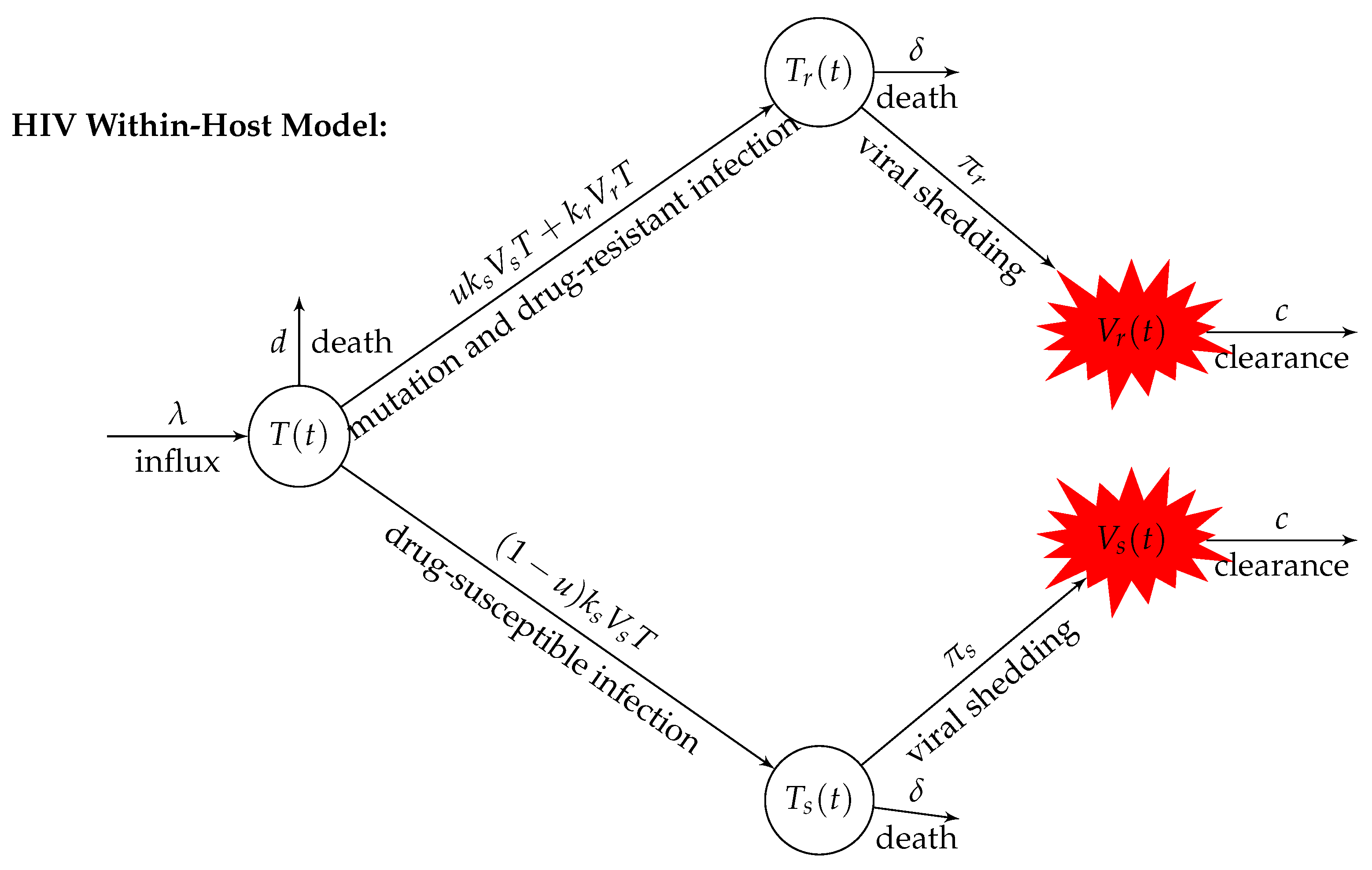
2. Model Formulation

HIV primarily targets and infects CD4⁺ T cells, which play an important role in the adaptive immune response. In return, infected CD4⁺ T cells produce HIV viral particles. For the dynamics of sensitive and resistant HIV, we used the following well-studied HIV within-host model [3,9].

$$\begin{array}{cc}\hfill {\displaystyle \frac{dT}{dt}}& =\lambda -dT-k_s{V}_{s}T-k_r{V}_{r}T\hfill \\ \hfill {\displaystyle \frac{d{T}_s}{dt}}& =(1-u)k_s{V}_{s}T-\delta T_s\hfill \\ \hfill {\displaystyle \frac{d{V}_s}{dt}}& ={\pi }_s{T}_s-c{V}_s\hfill \\ \hfill {\displaystyle \frac{d{T}_r}{dt}}& =u{k}_s{V}_{s}T+k_r{V}_{r}T-\delta T_r\hfill \\ \hfill {\displaystyle \frac{d{V}_r}{dt}}& ={\pi }_r{T}_r-c{V}_r\hfill \end{array}$$

(1)

These differential equations describe the dynamics of CD4⁺ T cells (T), cells infected with drug-resistant virus ($T_r$), cells infected with drug-susceptible virus ($T_s$), drug-resistant viral load ($V_r$), and drug-susceptible viral load ($V_s$). The parameter $\lambda$ represents the recruitment rate of uninfected CD4⁺ T cells, d is the per capita death rate of uninfected T-cells, and $k_r$ and $k_s$ are the infection rates of target cells by drug-resistant and drug-susceptible viruses, respectively. Regarding the interplay between susceptible and resistant strains of the virus, we set u ($0\le u<1$) to define the mutation rate from the sensitive strain to the resistant strain of the virus. ${\pi }_r$ and ${\pi }_s$ represent the burst sizes of the drug-resistant and drug-susceptible virus, respectively, which are the total number of virus particles released by a productive infected cell over its lifespan. c is the clearance rate of the virus, while $\delta$ is the death rate of infected CD4⁺ T cells.

Figure 1 depicts a flow diagram of the model. Table 1 lists the parameters and state variables of the within-host model (1).

Figure 1. Flow diagram describing the interaction between target cells $\left(T\right)$, infected cells with drug-resistant virus $\left(T_r\right)$, infected cells with drug-sensitive virus $\left(T_s\right)$, drug-sensitive virus $\left(V_s\right)$, and drug-resistant virus $\left(V_r\right)$.

Table 1. Definitions of the HIV within-host model (1) parameters and state variables and their units.

Parameter	Definition	Units
$\lambda$	Recruitment rate of uninfected target cells	$\mathrm{CD}{4}^{+}\mathrm{cells}{\mathrm{mL}}^{-1}{\mathrm{day}}^{-1}$
$k_s$	Infection rate of target cells by drug-sensitive virus	$\mathrm{mL}\mathrm{vRNA}{\mathrm{copies}}^{-1}{\mathrm{day}}^{-1}$
$k_r$	Infection rate of target cells by drug-resistant virus	$\mathrm{mL}\mathrm{vRNA}{\mathrm{copies}}^{-1}{\mathrm{day}}^{-1}$
u	Mutation rate from sensitive strain to resistant strain	$\mathrm{dimensionless}$
${\pi }_r$	Burst size of drug-resistant strain	${10}^{-3}\mathrm{vRNA}\mathrm{copies}{\left(\mathrm{CD}{4}^{+}\mathrm{cells}\mathrm{day}\right)}^{-1}$
${\pi }_s$	Burst size of drug-sensitive strain	${10}^{-3}\mathrm{vRNA}\mathrm{copies}{\left(\mathrm{CD}{4}^{+}\mathrm{cells}\mathrm{day}\right)}^{-1}$
c	Clearance rate of free virus	${\mathrm{day}}^{-1}$
$\delta$	Death rate of infected cells	${\mathrm{day}}^{-1}$
State Variable	Definition	Units
T	Population of Target (CD4+) Cells	$\mathrm{CD}{4}^{+}\mathrm{cells}$ per µL
$T_r$	Population of Infected Target (CD4+) Cells with Drug-Resistant Virus	$\mathrm{CD}{4}^{+}\mathrm{cells}$ per µL
$T_s$	Population of Infected Target (CD4+) Cells with Drug-Susceptible Virus	$\mathrm{CD}{4}^{+}\mathrm{cells}$ per µL
$V_r$	Drug-Resistant Viral Load	$\mathrm{vRNA}\mathrm{copies}{\mathrm{mL}}^{-1}$
$V_s$	Drug-Susceptible Viral Load	$\mathrm{vRNA}\mathrm{copies}{\mathrm{mL}}^{-1}$

3. Identifiability Analysis

Identifiability analysis is an assessment of whether a set of observations can be used to uniquely (structural identifiability) and accurately (practical identifiability) estimate model parameters. Within identifiability analysis, there are two sequential stages: (i) structural identifiability and (ii) practical identifiability. Structural identifiability is used to evaluate whether the parameters of a within-host model can be uniquely derived from infinitely many noise-free data. Structural identifiability analysis relies on the relation between a model and the observations. Consequently, structural identifiability analysis is a prerequisite for parameter estimation. If the model is structurally identifiable, then we may continue to estimate the parameters from the experimental data. Through practical identifiability analysis, one evaluates the parameters of the within-host model to see if they can be determined from experimental data with varying degrees of noise. There are a variety of methods utilized to study structural identifiability, including but not limited to the Taylor series approach [22], similarity transformation [23], generating series method [24], and the differential algebra approach [25,26]. Similarly, there are several methods to study practical identifiability of within-host models. These methods are profile likelihood [27], Monte Carlo simulations [19,28,29], and the Fisher Information Matrix (FIM) or Correlation Matrix [30,31,32]. In this study, we use the differential algebra method to study structural identifiability and the Monte Carlo simulations to examine the practical identifiability.

Structural Identifiability Analysis

We begin by assessing the structural identifiability of the within-host model and rewrite the model (1) in the following compact form:

$$\begin{array}{cc}\hfill x^{\prime }\left(t\right)& =f(x\left(t\right),p),x\left(0\right)=x_0\hfill \end{array}$$

(2)

$$\begin{array}{cc}\hfill y(t,p)& =g\left(x\right(t),p)\hfill \end{array}$$

(3)

Here, t represents time, x represents the state variables, and p represents the parameter vector with $p=(\lambda ,\delta ,c,d,k_s,k_r,{\pi }_r,{\pi }_s,u)$. We refer to $y(t,p)$ as observations; it is a smooth curve where the data are measured in discrete time. The observations, $y(t,p)$, are functions of the state variables. The within-host model given in compact form (2) is identifiable if the parameter vector p can be uniquely determined from the given observation $y(t,p)$, (3). Otherwise, it is said to be unidentifiable. To begin, we provide the definition of structural identifiability [19,29].

Definition 1.

• Globally identifiable: Let p and $\widehat{p}$ be two distinct parameter vectors. The model (2) is said to be structurally globally (uniquely) identifiable if

  $$g(x\left(t\right),p)=g(x\left(t\right),\widehat{p})\mathit{implies}p=\widehat{p}.$$
• Locally identifiable: The model (2) is said to be locally structurally locally identifiable if for any p within an open neighborhood of $\widehat{p}$ in the parameter space,

  $$g(x\left(t\right),p)=g(x\left(t\right),\widehat{p})\mathit{implies}p=\widehat{p}.$$

In AIDS clinical studies, the viral load and total CD4⁺ T-cell counts are usually measured. Therefore, in this study, we performed two the observations: the first one was the target cells, denoted by $y_1(t,p)$, and the second one was the total viral load, denoted by $y_2(t,p)$. With regard to the model variables, the observations can be written as follows:

$$\begin{array}{c}\hfill y_1(t,p)=T\left(t\right)+T_s\left(t\right)+T_r\left(t\right)\mathrm{and}{y}_2(t,p)=V_r\left(t\right)+V_s\left(t\right).\end{array}$$

(4)

To analyze the structural identifiability of the model, we utilized the differential algebra method [20]. The differential algebra method allows for the removal of the unobserved state variables, and by doing so, we derive an equation referred to as an input–output equation, which involves only the model parameters and observed state variables. The following input–output equations for model (1) with the observations $y_1(t,p)$ and $y_2(t,p)$ were obtained using the Differential Algebra for Identifiability of SYstem (DAISY v2.1) software [26]. The input–output equations of the system (1) with the observations (4) are the following monic differential polynomials (5) and (6).

$$\begin{array}{cc}\hfill 0& {\displaystyle =y_1^{″}+y_1^{\prime }{y}_2\frac{k_r{k}_s({\pi }_r-{\pi }_s)(1-u)}{{\pi }_r(k_r-k_{s}u)-k_s{\pi }_s(1-u)}+y_1^{\prime }(d+\delta )+y_2^{″}\frac{(d-\delta )(k_s-k_r)}{{\pi }_r(k_r-k_{s}u)-k_s{\pi }_s(1-u)}+}\hfill \\ \hfill & {\displaystyle y_2^{\prime }\frac{(c+\delta )(d-\delta )(k_s-k_r)}{{\pi }_r(k_r-k_{s}u)-k_s{\pi }_s(1-u)}+y_1{y}_2\frac{\delta k_r{k}_s({\pi }_r-{\pi }_s)(1-u)}{{\pi }_r(k_r-k_{s}u)-k_s{\pi }_s(1-u)}+y_{1}d\delta +}\hfill \\ \hfill & {\displaystyle y_2\frac{(cd\delta -c{\delta }^2)(k_s-k_r)+k_r{k}_s\lambda ({\pi }_r-{\pi }_s)(1-u)}{{\pi }_r(k_r-k_{s}u)-k_s{\pi }_s(1-u)}-\delta \lambda }\hfill \end{array}$$

(5)

and

$$\begin{array}{cc}\hfill 0& =y_1^{‴}{y}_1^{\prime }+y_1^{‴}{y}_1\delta -y_1^{‴}\lambda -y_1^{″2}+y_1^{″}{y}_1^{\prime }(c-\delta )+y_1^{″}{y}_1\delta (c+\delta )-y_1^{″}\lambda (c+d)+\hfill \\ \hfill & {\displaystyle y_1^{\prime 3}\frac{{\pi }_r{\pi }_s(k_s-k_r)}{(d-\delta )({\pi }_r-{\pi }_s)}+y_1^{\prime 2}{y}_2^{\prime }\frac{{\pi }_r{k}_r-{\pi }_s{k}_s}{{\pi }_r-{\pi }_s}+y_1^{\prime 2}{y}_1\frac{{\pi }_r{\pi }_s(k_s-k_r)(d+2\delta )}{(d-\delta )({\pi }_r-{\pi }_s)}+}\hfill \\ \hfill & {\displaystyle y_1^{\prime 2}{y}_2\frac{c({\pi }_r{k}_r-{\pi }_s{k}_s)}{{\pi }_r-{\pi }_s}+y_1^{\prime 2}(c(d+\delta )-{\delta }^2+\frac{3\lambda {\pi }_r{\pi }_s(k_s-k_r)}{(d-\delta )({\pi }_r-{\pi }_s)})+y_1^{\prime }{y}_2^{\prime }{y}_1\frac{2\delta ({\pi }_r{k}_r-{\pi }_s{k}_s)}{{\pi }_r-{\pi }_s}+}\hfill \\ \hfill & {\displaystyle y_1^{\prime }{y}_2^{\prime }\frac{2\lambda ({\pi }_r{k}_r-{\pi }_s{k}_s)}{{\pi }_r-{\pi }_s}+y_1^{\prime }{y}_1^2\frac{\delta (2d-\delta ){\pi }_r{\pi }_s(k_s-k_r)}{(d-\delta )({\pi }_r-{\pi }_s)}+}\hfill \\ \hfill & {\displaystyle y_1^{\prime }{y}_1{y}_2\frac{2c\delta ({\pi }_r{k}_r-{\pi }_s{k}_s)}{{\pi }_r-{\pi }_s}+y_1^{\prime }{y}_1\left({\displaystyle \frac{2c{d}^2\delta -cd{\delta }^2-c{\delta }^3}{d-\delta }+\frac{(2d\lambda +4\delta \lambda ){\pi }_r{\pi }_s(k_s-k_r)}{(d-\delta )({\pi }_r-{\pi }_s)}}\right)-}\hfill \\ \hfill & {\displaystyle y_1^{\prime }{y}_2\frac{2c\lambda ({\pi }_r{k}_r-{\pi }_s{k}_s)}{{\pi }_r-{\pi }_s}+y_1^{\prime }\left({\displaystyle \frac{c{d}^2-cd\delta +2c{\delta }^2-d^2\delta +2d{\delta }^2-{\delta }^3}{d-\delta }-\frac{3\lambda {\pi }_r{\pi }_s(k_s-k_r)}{(d-\delta )({\pi }_r-{\pi }_s)}}\right)+}\hfill \\ \hfill & {\displaystyle y_2^{\prime }{y}_1^2\frac{{\delta }^2({\pi }_r{k}_r-{\pi }_s{k}_s)}{{\pi }_r-{\pi }_s}+y_2^{\prime }{y}_1\frac{2\delta \lambda ({\pi }_r{k}_r-{\pi }_s{k}_s)}{{\pi }_r-{\pi }_s}+y_2^{\prime }\frac{{\lambda }^2({\pi }_r{k}_r-{\pi }_s{k}_s)}{{\pi }_r-{\pi }_s}+}\hfill \\ \hfill & {\displaystyle y_1^3\frac{d{\delta }^2{\pi }_r{\pi }_s(k_s-k_r)}{(d-\delta )({\pi }_r-{\pi }_s)}+y_1^2{y}_2\frac{c{\delta }^2({\pi }_r{k}_r-{\pi }_s{k}_s)}{{\pi }_r-{\pi }_s}+y_1^2\left({\displaystyle 2cd{\delta }^2+\frac{(2d\lambda +\delta \lambda ){\pi }_r{\pi }_s(k_s-k_r)}{(d-\delta )({\pi }_r-{\pi }_s)}}\right)+}\hfill \\ \hfill & {\displaystyle y_1{y}_2\frac{2c\delta \lambda ({\pi }_r{k}_r-{\pi }_s{k}_s)}{{\pi }_r-{\pi }_s}+y_1\left({\displaystyle -c\delta (d+\delta )-\frac{\lambda (d-2\delta ){\pi }_r{\pi }_s(k_s-k_r)}{(d-\delta )({\pi }_r-{\pi }_s)}}\right)+}\hfill \\ \hfill & {\displaystyle y_2\frac{c{\lambda }^2({\pi }_r{k}_r-{\pi }_s{k}_s)}{{\pi }_r-{\pi }_s}+\left({\displaystyle {\lambda }^{2}c\delta +\frac{\lambda {\pi }_r{\pi }_s(k_s-k_r)}{(d-\delta )({\pi }_r-{\pi }_s)}}\right).}\hfill \end{array}$$

(6)

Solving the differential polynomials (5) and (6) is equivalent to solving the within-host model (1) for $y_1(t,p)$ and $y_2(t,p)$. Therefore, the definition of the structural identifiability within differential algebra approach becomes verifying that the coefficients of the differential polynomials (5) and (6) are one-to-one with respect to the parameters [18,19,20,33].

Definition 2.

Let $c\left(p\right)$ denote the coefficients of the input–output Equations (5) and (6), where p is the vector of model parameters. The within-host model is said to be structurally identifiable, that is, it is structured to reveal its parameters from the observations $y_1(t,p)$ and $y_2(t,p)$ if and only if

$$\begin{array}{c}\hfill c\left(p\right)=c\left(\widehat{p}\right)⟹p=\widehat{p}\end{array}$$

(7)

According to Definition 2, we must show that the mapping of the parameter space to the coefficients is one-to-one. Let us suppose that there is a parameter vector $\widehat{p}=(\widehat{\lambda },\widehat{\delta },\widehat{c},\widehat{d},{\widehat{k}}_s,{\widehat{k}}_r,{\widehat{\pi }}_r,{\widehat{\pi }}_s,\widehat{u})$ that produces the same target cell and viral load observations. Then, setting $c\left(p\right)=c\left(\widehat{p}\right)$, we obtain the following system of nonlinear equations:

$$\begin{array}{cc}\hfill & \delta =\widehat{\delta }\hfill \\ \hfill & \lambda =\widehat{\lambda }\hfill \\ \hfill & c-\delta =\widehat{c}-\widehat{\delta }\Rightarrow c=\widehat{c}\hfill \\ \hfill & c+d=\widehat{c}+\widehat{d}\Rightarrow d=\widehat{d}\hfill \\ \hfill & {\displaystyle \frac{k_r{k}_s({\pi }_r-{\pi }_s)(1-u)}{{\pi }_r(k_r-k_{s}u)-k_s{\pi }_s(1-u)}=\frac{{\widehat{k}}_r{\widehat{k}}_s({\widehat{\pi }}_r-{\widehat{\pi }}_s)(1-\widehat{u})}{{\widehat{\pi }}_r({\widehat{k}}_r-{\widehat{k}}_s\widehat{u})-{\widehat{k}}_s{\widehat{\pi }}_s(1-\widehat{u})}}\hfill \\ \hfill & {\displaystyle \frac{(k_s-k_r)}{{\pi }_r(k_r-k_{s}u)-k_s{\pi }_s(1-u)}=\frac{({\widehat{k}}_s-{\widehat{k}}_r)}{{\widehat{\pi }}_r({\widehat{k}}_r-{\widehat{k}}_s\widehat{u})-{\widehat{k}}_s{\widehat{\pi }}_s(1-\widehat{u})}}\hfill \\ \hfill & {\displaystyle \frac{{\pi }_r{\pi }_s(k_s-k_r)}{{\pi }_r-{\pi }_s}=\frac{{\widehat{\pi }}_r{\widehat{\pi }}_s({\widehat{k}}_s-{\widehat{k}}_r)}{{\widehat{\pi }}_r-{\widehat{\pi }}_s}}\hfill \\ \hfill & {\displaystyle \frac{{\pi }_r{k}_r-{\pi }_s{k}_s}{{\pi }_r-{\pi }_s}=\frac{{\widehat{\pi }}_r{\widehat{k}}_r-{\widehat{\pi }}_s{\widehat{k}}_s}{{\widehat{\pi }}_r-{\widehat{\pi }}_s}}\hfill \end{array}$$

(8)

Here, we note that the DAISY addresses the nonlinear system of Equations (8) by substituting random integer values for the parameters $\widehat{p}$. However, those solutions given by DAISY are not clearly stating the parameter correlations. Furthermore, $0\le u<1$ is not an integer; such integer solutions can not be accepted. Therefore, we used Wolfram Mathematica to solve this nonlinear system (8) and obtained the following:

$S_1=\{\lambda =\widehat{\lambda },\delta =\widehat{\delta },c=\widehat{c},d=\widehat{d},k_r=k_s,{\pi }_r={\pi }_s\}$

$$\begin{gathered} S_2=\left\{{\displaystyle \lambda =\widehat{\lambda },\delta =\widehat{\delta },c=\widehat{c},d=\widehat{d},k_r={\widehat{k}}_r,{\pi }_s=\frac{({\widehat{k}}_r-{\widehat{k}}_s){\widehat{\pi }}_r{\widehat{\pi }}_s}{({\widehat{k}}_r{\widehat{\pi }}_r-k_s{\widehat{\pi }}_r+k_s{\widehat{\pi }}_s-{\widehat{k}}_s{\widehat{\pi }}_s)},}\right. \\ \left.{\displaystyle {\pi }_r={\widehat{\pi }}_r,u=\frac{({\widehat{k}}_r{\widehat{\pi }}_r(k_s-{\widehat{k}}_s(1-\widehat{u}))+{\widehat{k}}_s({\widehat{k}}_s{\widehat{\pi }}_s(1-\widehat{u})-k_s({\widehat{\pi }}_s(1-\widehat{u})+{\widehat{\pi }}_r\widehat{u})))}{\left(k_s({\widehat{k}}_r-{\widehat{k}}_s){\widehat{\pi }}_r\right)}}\right\} \end{gathered}$$

$$\begin{gathered} S_3=\left\{{\displaystyle \lambda =\widehat{\lambda },\delta =\widehat{\delta },c=\widehat{c},d=\widehat{d},k_r=\frac{{\widehat{k}}_s({\widehat{k}}_r{\widehat{\pi }}_r-{\widehat{k}}_s{\widehat{\pi }}_s)(1-\widehat{u})}{(-{\widehat{k}}_r{\widehat{\pi }}_r+{\widehat{k}}_s{\widehat{\pi }}_s(1-\widehat{u})+{\widehat{k}}_s{\widehat{\pi }}_r\widehat{u})},}\right. \\ {\displaystyle {\pi }_s=\frac{({\widehat{k}}_r-{\widehat{k}}_s){\widehat{\pi }}_r{\widehat{\pi }}_s}{({\widehat{k}}_r{\widehat{\pi }}_r-k_s{\widehat{\pi }}_r+k_s{\widehat{\pi }}_s-{\widehat{k}}_s{\widehat{\pi }}_s)},{\pi }_r=\frac{\left({\widehat{\pi }}_s({\widehat{k}}_r{\widehat{\pi }}_r-{\widehat{k}}_s{\widehat{\pi }}_s(1-\widehat{u})-{\widehat{k}}_s{\widehat{\pi }}_r\widehat{u})\right)}{({\widehat{k}}_r{\widehat{\pi }}_r-{\widehat{k}}_s{\widehat{\pi }}_s)},} \\ \left.{\displaystyle u=\frac{(k_s-{\widehat{k}}_r)({\widehat{k}}_r{\widehat{\pi }}_r-{\widehat{k}}_s{\widehat{\pi }}_s)}{k_s{\widehat{\pi }}_s({\widehat{k}}_r-{\widehat{k}}_s)}}\right\} \end{gathered}$$

We obtained three sets of solutions; $S_1,S_2$, and $S_3$, each displaying several parameter correlations. The parameters $\lambda ,\delta ,c$, and d can be identified, but complex correlations exist between the parameters $k_s,k_r,{\pi }_s,{\pi }_r$, and u. It is clear that the within-host model is not structurally identifiable. Upon further inspection, we notice that the solution set $S_3$ is inadmissible. To show that $S_3$ is not an acceptable solution, we multiply $k_r$ and ${\pi }_r$ in $S_3$ and obtain the following:

$$\begin{array}{cc}\hfill & {\displaystyle k_r\times {\pi }_r=\frac{\left({\widehat{k}}_s({\widehat{k}}_r{\widehat{\pi }}_r-{\widehat{k}}_s{\widehat{\pi }}_s)(1-\widehat{u})\right)}{(-{\widehat{k}}_r{\widehat{\pi }}_r+{\widehat{k}}_s{\widehat{\pi }}_s+{\widehat{k}}_s{\widehat{\pi }}_r\widehat{u}-{\widehat{k}}_s{\widehat{\pi }}_s\widehat{u})}\times \frac{\left({\widehat{\pi }}_s({\widehat{k}}_r{\widehat{\pi }}_r+{\widehat{k}}_s{\widehat{\pi }}_s(-1+\widehat{u})-{\widehat{k}}_s{\widehat{\pi }}_r\widehat{u})\right)}{({\widehat{k}}_r{\widehat{\pi }}_r-{\widehat{k}}_s{\widehat{\pi }}_s)}}\hfill \\ \hfill & {\displaystyle =\frac{{\widehat{k}}_s(1-\widehat{u})}{-({\widehat{k}}_r{\widehat{\pi }}_r-{\widehat{k}}_s{\widehat{\pi }}_s-{\widehat{k}}_s{\widehat{\pi }}_r\widehat{u}+{\widehat{k}}_s{\widehat{\pi }}_s\widehat{u})}\times \left({\widehat{\pi }}_s({\widehat{k}}_r{\widehat{\pi }}_r+{\widehat{k}}_s{\widehat{\pi }}_s(-1+\widehat{u})-{\widehat{k}}_s{\widehat{\pi }}_r\widehat{u})\right)}\hfill \\ \hfill & {\displaystyle =\frac{{\widehat{k}}_s(1-\widehat{u})}{-({\widehat{k}}_r{\widehat{\pi }}_r+{\widehat{k}}_s{\widehat{\pi }}_s(-1+\widehat{u})-{\widehat{k}}_s{\widehat{\pi }}_r\widehat{u})}\times \left({\widehat{\pi }}_s({\widehat{k}}_r{\widehat{\pi }}_r+{\widehat{k}}_s{\widehat{\pi }}_s(-1+\widehat{u})-{\widehat{k}}_s{\widehat{\pi }}_r\widehat{u})\right)}\hfill \\ \hfill & =-{\widehat{k}}_s{\widehat{\pi }}_s(1-\widehat{u})\hfill \end{array}$$

We obtain $k_r{\pi }_r=-{\widehat{k}}_s{\widehat{\pi }}_s(1-\widehat{u})$, which means that $k_r{\pi }_r<0$ since $0<\widehat{u}<1$. As such, either $k_r$ or ${\pi }_r$ must be negative, which is not possible since all parameters in our model have positive values. Therefore, solution set $S_3$ is not an admissible solution. We summarize the structural identifiability results in the following Proposition 1.

Proposition 1.

As evident by solution sets $S_1$ and $S_2$, the within-host model (1) is not structured to reveal its parameters from the observations of target cell count, $y_1\left(t\right)=T\left(t\right)+T_s\left(t\right)+T_r\left(t\right)$, and viral load measurements, $y_2\left(t\right)=V_r\left(t\right)+V_s\left(t\right)$.

Our goal is to obtain a structurally identifiable model from the observations of target cell count and viral load measurements. We can achieve this goal in two different ways and present these two ways in this study: (1) fix some parameters so that the remaining parameters become structurally identifiable or (2) add more information, namely, observations, to the identifiability analysis. Let us explore the first approach. First, we fix the rate at which infected cells with sensitive HIV produce new viral particles per day, namely, the parameter ${\pi }_s$. We also impose that the rate at which infected cells with resistant HIV produce new viral particles is different from the infected cells with sensitive HIV. Therefore, we add ${\pi }_s={\widehat{\pi }}_s$ and ${\pi }_r\ne {\pi }_s$ to the system of nonlinear equations $c\left(p\right)=c\left(\widehat{p}\right)$ given in (8). We solved the system in Mathematica and obtain the following solution:

$$\begin{array}{cc}\hfill L_1=\{& \lambda =\widehat{\lambda },\delta =\widehat{\delta },c=\widehat{c},d=\widehat{d},u=\widehat{u},{\pi }_s={\widehat{\pi }}_s,\hfill \\ \hfill & k_s={\widehat{k}}_s,k_r={\widehat{k}}_r,{\pi }_r={\widehat{\pi }}_r\}\hfill \\ \hfill L_2=\{& \lambda =\widehat{\lambda },\delta =\widehat{\delta },c=\widehat{c},d=\widehat{d},k_s={\widehat{k}}_s,{\pi }_s={\widehat{\pi }}_s,\hfill \\ \hfill & k_r={\displaystyle \frac{{\widehat{k}}_s({\widehat{k}}_r{\widehat{\pi }}_r-{\widehat{k}}_s{\widehat{\pi }}_s)(1-\widehat{u})}{{\widehat{\pi }}_r({\widehat{k}}_s\widehat{u}-{\widehat{k}}_r)+{\widehat{k}}_s{\widehat{\pi }}_s(1-\widehat{u})}},{\pi }_r={\displaystyle \frac{{\widehat{\pi }}_r({\widehat{\pi }}_r({\widehat{k}}_s\widehat{u}-{\widehat{k}}_r)+{\widehat{k}}_s{\widehat{\pi }}_s(1-\widehat{u}))}{{\widehat{k}}_r{\widehat{\pi }}_r-{\widehat{k}}_s{\widehat{\pi }}_s}},\hfill \\ \hfill & u=1-{\displaystyle \frac{{\widehat{k}}_r{\widehat{\pi }}_r}{{\widehat{k}}_s{\widehat{\pi }}_s}}\}\hfill \end{array}$$

A closer look at the solution set $L_2$ reveals that ${\pi }_r{k}_r=-{\displaystyle \frac{{\widehat{k}}_s}{{\widehat{\pi }}_r}}(1-\widehat{u})$. Since u is less than one and all the parameters are positive, the equality gives the product of the parameters ${\pi }_r$ and $k_r$ to be negative, which is not possible. Therefore, the set $L_2$ is not admissible for the HIV model (1). We can only accept solution set $L_1$, which yields a structurally identifiable model. We summarize the results in the following Proposition 2.

Proposition 2.

If the viral busting rate ${\pi }_s$ of CD4⁺ T-cells infected with sensitive virus is known, and if we further impose that ${\pi }_s$ and ${\pi }_r$ are not identical, then the within-host model (1) is structured to reveal its parameters from the observations of target cell count and viral load measurements.

Now, we explore the second approach to obtaining a structurally identifiable within-host model, that is, adding more data, hence observations, to the identifiability analysis. In an AIDS clinical study, it is not possible to measure the infected CD4⁺ T cells separately, meaning that the number of CD4⁺ T cell count includes both healthy and infected cells. On the other hand, we found that in this AIDS clinical studies [3,8], drug-sensitive and drug-resistant viral loads are measured separately. Therefore, the observations in this AIDS clinical study take the form of the number of target cells, denoted by $y_1(t,p)$, the drug-sensitive viral load, denoted by $y_2(t,p)$, and the drug-resistant viral load, denoted by $y_3(t,p)$. With regard to the model (1) variables, the observations can be written as follows:

$$\begin{array}{c}\hfill y_1(t,p)=T\left(t\right)+T_s\left(t\right)+T_r\left(t\right)\mathrm{and}{y}_2(t,p)=V_s\left(t\right)\mathrm{and}{y}_3(t,p)=V_r\left(t\right)\end{array}$$

(9)

For within-host model (1) and the observations (9), DAISY gives the following set of input–output equations:

$$\begin{array}{cc}\hfill & 0=y_1^{\prime }-y_2^{\prime }{\displaystyle \frac{(d-\delta )}{{\pi }_s}}-y_3^{\prime }{\displaystyle \frac{(d-\delta )}{{\pi }_r}}+y_{1}d-y_2{\displaystyle \frac{c(d-\delta )}{{\pi }_s}}-y_3{\displaystyle \frac{c(d-\delta )}{{\pi }_r}}-\lambda \hfill \\ \hfill & 0=y_1^{″}+y_1^{\prime }{y}_2{k}_s+y_1^{\prime }{y}_3{k}_r+y_1^{\prime }(d+\delta )+y_1{y}_2{k}_s\delta +y_1{y}_3{k}_r\delta +y_{1}d\delta -\hfill \\ \hfill & y_2{k}_s\lambda -y_3{k}_r\lambda -\delta \lambda \hfill \\ \hfill & 0=y_1^{\prime }{y}_2{\displaystyle \frac{k_s{\pi }_s(1-u)}{(d-\delta )}}+y_2^{″}+y_2^{\prime }(c+\delta )+y_1{y}_2{\displaystyle \frac{k_s\delta {\pi }_s(1-u)}{d-\delta }}\hfill \\ \hfill & +y_2{\displaystyle \frac{(k_s\lambda {\pi }_{s}u-k_s\lambda {\pi }_s+cd\delta -c{\delta }^2)}{d-\delta }}\hfill \end{array}$$

Applying Definition 2, we set $c\left(p\right)=c\left(\widehat{p}\right)$ and obtain the following solution:

$$\begin{array}{cc}\hfill & \lambda =\widehat{\lambda },\delta =\widehat{\delta },c=\widehat{c},d=\widehat{d},u=\widehat{u},{\pi }_s={\widehat{\pi }}_s,k_s={\widehat{k}}_s,\hfill \\ \hfill & k_r={\widehat{k}}_r,{\pi }_r={\widehat{\pi }}_r.\hfill \end{array}$$

This means that the within-host model (1) is structured to reveal its parameters from the observations of total CD⁺ T-cell count, drug-sensitive HIV load, and drug-resistant HIV load. We state the following Proposition 3.

Proposition 3.

The within-host model (1) is structurally identifiable from the observations of target cell count, $y_1\left(t\right)=T\left(t\right)+T_s\left(t\right)+T_r\left(t\right)$, drug-sensitive viral load $y_2\left(t\right)=V_s\left(t\right)$, and drug-resistant viral load $y_3\left(t\right)=V_r\left(t\right)$ measurements.

4. Parameter Estimation and Data

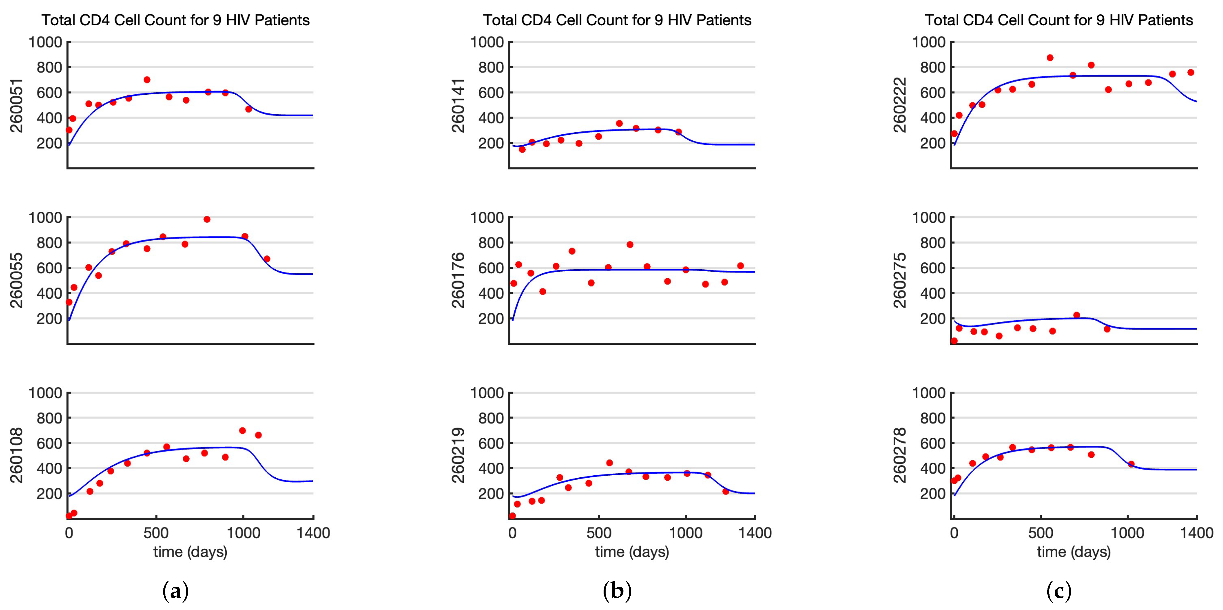
4.1. Estimating Model Parameters from AIDS Clinical Trial Data Set with Nine Patients

Data Set 1: To estimate the parameters of the within-host model (1), we used the data from the Stanford HIV Drug Resistance Database [34]. Specifically, we used the data collected from the AIDS Clinical Trial Groups (ACTG) 5257 [35]. The ACTG 5257 study was performed on treatment-naive people over the age of 18 who had HIV-1 RNA levels of over 1000 copies/mL. More than 1800 participants were enrolled in the study with a median age of 37, $24\%$ being women. CD8 T cell count was not reported in the study. Virologic failure was defined as RNA levels greater than 1000 copies/mL after 16 weeks and before 24 weeks or 200 copies/mL at or after 24 weeks. It is reported that among those who received the non-nucleoside reverse transcriptase inhibitor (NNRT) Raltegravir, $3\%$ experienced virologic failure as a result of drug resistance [35]. From the data set of this study, we chose 9 patients who were on NNRT and protease inhibitor (PI) regimens and showing viral failure. However, it is important to note that there is no evidence that these specific 9 patients experienced virologic failure as a result of developing resistance. In principle, virologic failure may occur as a result of different reasons such as the patient not following the prescribed medication regimen.

• Estimating Model Parameters From Data Set 1: Since we had data from 9 HIV infected individuals from the AIDS clinical data set [35], to estimate the parameters of the within-host model (1), we used the nonlinear mixed effect modeling approach. The nonlinear mixed effect model is defined

  $$\begin{array}{cc}\hfill y_{i,j}^1& =y_1(t_j,p_i)+c_1{y}_1{(t_j,p_i)}^{\xi }{ϵ}_{i,j}{ϵ}_{ij}\sim N(0,{\sigma }^2)\hfill \end{array}$$

  (10)

  $$\begin{array}{cc}\hfill y_{i,j}^2& =y_2(t_j,p_i)+c_2{y}_2{(t_j,p_i)}^{\xi }{ϵ}_{i,j}{ϵ}_{ij}\sim N(0,{\sigma }^2)\hfill \end{array}$$

  (11)

  where $y_1(t_j,p_i)$ is the model prediction of total CD4⁺ T-cell counts at time $t_j$ of the ith individual, and $y_{i,j}^1$ is the CD4⁺ T-cell count of the ith individual at time $t_j$. Similarly, $y_2(t_j,p_i)$ is the model prediction of the total viral load on log scale at time $t_j$ of the ith individual, and $y_{i,j}^2$ is the log scale viral load data of the ith individuals at time $t_j$. The terms $c_1{y}_1{(t_j,p_i)}^{\xi }$ and $c_2{y}_2{(t_j,p_i)}^{\xi }$ represent the statistical error models. In most cases, $\xi =0$, which corresponds to the constant (or additive) error model, and when $\xi =1$, it is called the relative (proportional) error model. We assume that the total CD4⁺ T-cell count follows an additive error model, while the viral load data follow a relative error model. The $p_i=(\lambda ,\delta ,c,d,k_s,k_r,{\pi }_r,{\pi }_s,u)$ is the parameter vector for the ith individual. The random effect is then defined as

  $$p_i=\tilde{p}+{\eta }_i{\eta }_i\sim N(0,{\omega }_i^2)$$

  where $\tilde{p}$ is the fixed population parameter, and ${\eta }_i$ is the random effect. The individual parameters $p_i$ follow a normal distribution whose mean is the fixed population parameter $\tilde{p}$, and the standard deviation is ${\omega }_i$.

We use the stochastic approximation estimation-maximization (SAEM) algorithm in Monolix [21] to estimate the mean and standard deviation of parameters $p_i$. We assume that the individual parameters $p_i$ are log-normally distributed, with mean $ln\left(\tilde{p}\right)$ and standard deviation ${\omega }_i$. We set the initial drug-resistant viral load to zero and further set the initial number of infected cells with sensitive and resistant viruses to zero. Hence, $V_r\left(0\right)=0$ viral RNA copies per mL, $T_s\left(0\right)=0$, $T_r\left(0\right)=0$ cells per µL. Seven of the nine HIV-positive patients had a known total target cell count at time t = 0, which ranges between 20 and 308 cells per microliter. Therefore, we set the initial target cell count to the mean of the 7 patients and set $T\left(0\right)=178$ cells per µL, and we set the initial sensitive viral load, $V_s\left(0\right)=5204600$ viral RNA copies/mL, to the mean of the 9 patients. The structural identifiability analysis indicates that fixing the parameter ${\pi }_s$ is necessary to determine the remaining parameters uniquely. Therefore, we set ${\pi }_s=4.57$ viral RNA copies per cell per day. The estimated values for each patient ($p_i$) and the fixed population parameters ($\tilde{p}$) and their standard deviations (${\omega }_i$) are presented in Table 2.

Table 2. Monolix parameter estimation results for each HIV-infected individual and the fixed population parameters and their standard deviations.

Patient ID	$\mathit{\lambda }$	d	${\mathit{k}}_{\mathit{s}}$	${\mathit{k}}_{\mathit{r}}$	${\mathit{\pi }}_{\mathit{r}}$	c	$\mathit{\delta }$	u
260108	3.1432	0.0052	1.7003 × 10−5	2.0280 × 10−5	14.2923	2.6698	0.0151	2.2205 × 10−16
260176	8.5243	0.0146	1.7020 × 10−5	2.0086 × 10−5	13.9616	3.0708	0.0153	2.2205 × 10−16
260141	2.2569	0.0070	1.7086 × 10−5	2.2728 × 10−5	14.8627	1.5793	0.0153	2.2205 × 10−16
260051	5.3588	0.0086	1.7076 × 10−5	2.2009 × 10−5	14.3102	3.1006	0.0152	2.2205 × 10−16
260055	6.7139	0.0077	1.7129 × 10−5	2.0807 × 10−5	13.5409	4.1148	0.0153	2.2205 × 10−16
260275	1.4573	0.0069	1.7190 × 10−5	2.4921 × 10−5	16.3691	1.0295	0.0155	2.2205 × 10−16
260219	2.1811	0.0057	1.7189 × 10−5	2.0317 × 10−5	13.8618	1.7939	0.0154	2.2205 × 10−16
260222	6.2164	0.0082	1.7144 × 10−5	1.9117 × 10−5	12.9615	3.5886	0.0152	2.2205 × 10−16
260278	5.0414	0.0086	1.7000 × 10−5	2.2101 × 10−5	14.7130	2.8675	0.0153	2.2205 × 10−16
$\tilde{p}$	3.86	0.0075	0.000017	0.000022	14.12	2.42	0.015	2.2205 × 10−16
${\omega }_i$	0.6	0.36	0.025	0.11	0.11	0.42	0.031	3.58

Table 2 shows that infected CD4⁺ T cells die at a higher rate than uninfected cells, which is consistent with prior findings. The half-lives of uninfected cells are 92 days on average, and infected cells are 46 days, based on the fixed population estimates $\tilde{d}$ and $\tilde{\delta }$ ($ln\left(2\right)/0.0075=92$ and $ln\left(2\right)/0.015=46$). The clearance rate of HIV is $\tilde{c}=2.42$ per day, giving a half-life of 7 h. For the 9 HIV-infected individuals, the production rate of CD4⁺ T cells ranged from $1.46$ to $8.52$ cells per day per milliliter of blood. CD4⁺ cells infected with a resistant virus produce $14.12$ viral RNA copies per cell per day, higher than the cells infected with a sensitive virus. The infection rate of the resistant virus (${\tilde{k}}_r=2.2\times {10}^{-5}$ per viral particle per day in a mL blood) was larger than the infection rate of the sensitive virus (${\tilde{k}}_s=1.7\times {10}^{-5}$ per viral particle per day in a mL blood). All nine HIV patients had an estimated mutation rate of zero. This implies that mutation occurs at a single time rather than continually. Drug-resistance mutations are probably best modeled as a dirac-delta function.

Figure 2 shows predictions for each patient using the within-host model (1) with the parameters given in Table 2. We present the total viral load prediction by the within-host model (1) in Figure 2a, resistant viral load prediction in Figure 2b, and sensitive viral load in Figure 2c. After starting NNRT and PI antiviral therapy, patients’ total viral load clearly stays below 100 (2 on log scale) viral RNA copies. However, about two years into the treatment, virologic failure is detected (see dashed lines in Figure 2a). Furthermore, in all nine individuals, the resistant virus fully eliminated the sensitive virus. Despite following the same NNRT and PI regimen, the nine patients had significantly different total CD4⁺ cell counts (see Figure 3).

Figure 2. Monolix fitting results for 9 HIV infected patients. In columns (a–c), the red dots are the total viral load in log scale, including both the sensitive and resistant strains. (a) presents the within-host model (1) prediction of the total viral load in log scale (blue lines) together with the data. The dashed line gives the time when the total viral load exceeds 200 viral RNA copies per mL. (b) presents the within-host model (1) prediction of the resistant virus and the data. The dashed line gives the time when the resistant virus first appears in the system. (c) presents the within-host model (1) prediction of the sensitive virus together with the data.

Figure 3. Monolix fitting results for 9 HIV infected patients. In columns (a–c), the red dots are the total CD4⁺ cell count, including the cells infected with both the sensitive and resistant strains. In columns (a–c), the blue curve is the within-host model (1) prediction of the total CD4⁺ cell count.

The dashed line in Figure 2a indicates the time of virologic failure as defined by the clinical trial authors [35]. Specifically, it shows the point at which, after 24 weeks of antiretroviral therapy, the overall viral load surpasses 200 viral RNA levels. However, the point at which the patient first exhibits the resistant virus is marked by the dashed line in Figure 2b. We see at least a 100-day relapse between the initial emergence of the resistant virus and the detection of virologic failure for each patient. We present in Figure 4 the distribution of these time points. Patients develop resistant viruses on average 844 days after the initiation of the treatment, but detection occurs 970 days after.

Figure 4. The left-hand-side figure presents the distribution of the time points at which the resistant virus first appeared (see Figure 2b). The right-hand-side figure presents the distribution of the time points at which virologic failure is detected (see Figure 2a). Bars represent the empirical distributions, and the red curve is the theoretical distribution. Dashed lines are the mean of the distributions.

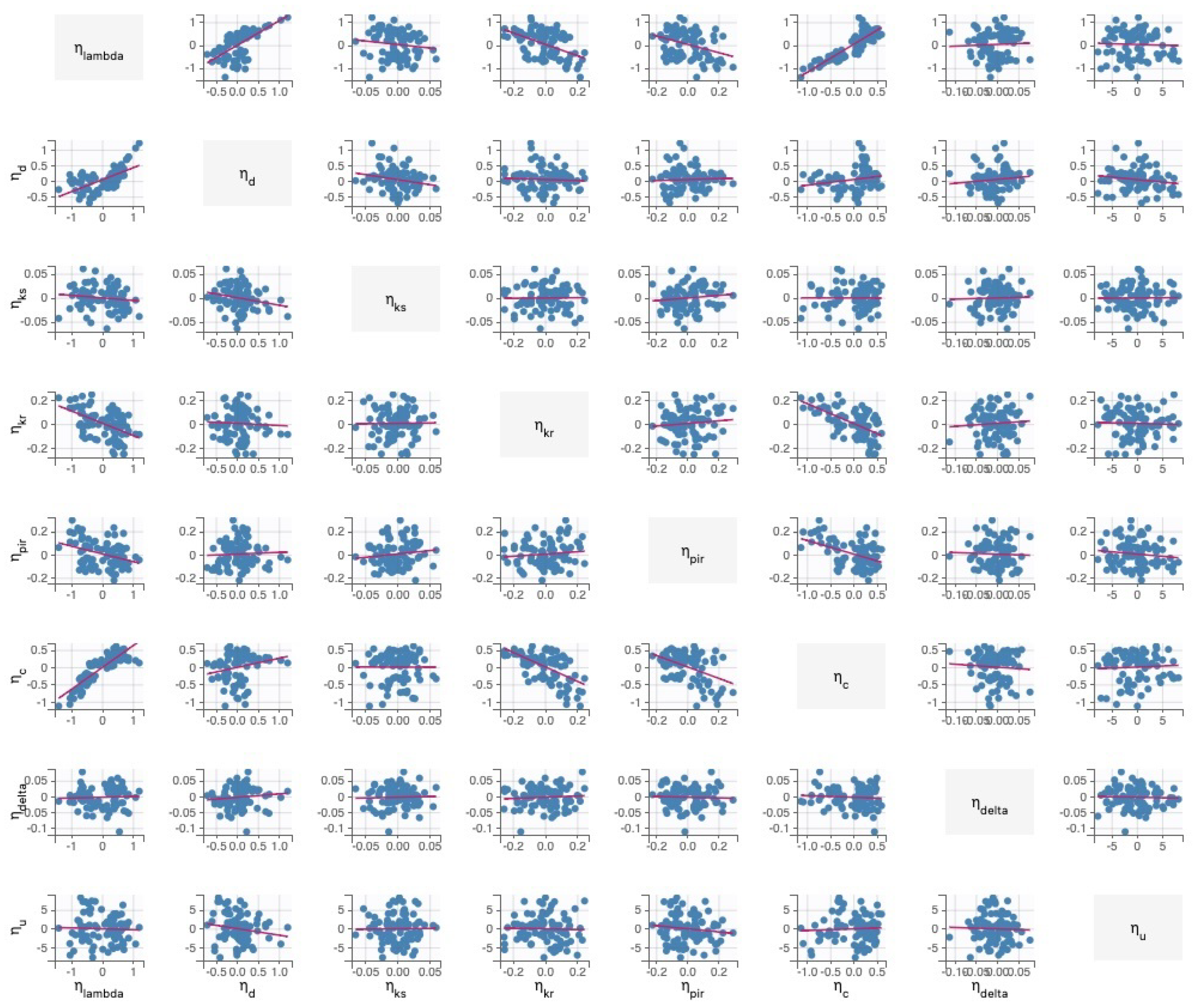
Practical Identifiability Analysis

Monolix provides the distribution of the parameters obtained by fitting the within-host model to the AIDS clinical trial data (see Figure 5), as well as the correlations between the random effects $\eta$ (see Figure A1). Figure A1 indicates that the parameter $\lambda$ is correlated with $c,d,k_r$ and ${\pi }_r$. These parameters also exhibit bimodal distributions (refer to Figure 5), particularly for $\lambda$ and c. The parameters $\lambda$ and c have the highest Pearson correlation coefficient ($0.88$). The correlation between parameters $\lambda$ and d is substantial with a Pearson coefficient of $0.64$. The Pearson correlation between parameters $\lambda$ and $k_r$ is $-0.51$, while that for $\lambda$ and ${\pi }_r$ is $-0.31$. The correlation threshold for claiming that a parameter is practically unidentifiable based on the Pearson coefficient is unclear. Based on our earlier studies [30], we claim that the parameters $\lambda$ and c are practically unidentifiable from fitting the within-host model (1) to the AIDS clinical trial data with nonlinear mixed effect modeling.

Figure 5. Parameter distribution generated by fitting within-host model (1) to the total viral load and total CD4⁺ cell count data.

4.2. Estimating Model Parameters from Published Data with Single HIV Patient

• Data Set 2: Our structural identifiability analysis shows that measuring sensitive and resistant viral loads separately can uniquely determine the parameters of the within-host model (1). However, we failed to find any AIDS clinical trials in the Stanford HIV Drug Resistance Database [34] that assessed both resistant and sensitive viruses individually. On the other hand, we did find a clinical trial with data published in [3] where the resistant and sensitive virus were measured separately. We used the published data in [3] where HIV-infected individuals were prescribed with the non-nucleoside reverse transcriptase (NNRT) inhibitor Nevirapine (NVP), and their response to the medication was assessed at specific time points: 0, 14, 28, 56, and 140 days after initiating therapy. During these evaluations, the total CD4+ T-cell count per µL was measured, along with the presence of HIV strains (per µL plasma) that are sensitive or resistant to NVP [3].

We fit the within-host model (1) using two separate data sets, each with distinct characteristics. To begin, in clinical study [35], data are available for around 1400 days, nearly 4 years, whereas in study [3], data are only available for 140 days (roughly 0.4 year). While it takes two years of treatment for the viral failure to develop in [35], in [3] it happens in just fourteen days. Furthermore, the total CD4⁺ cell count in [3] is very small compared to the same data in [35]. The HIV viral RNA copies are measured in a mililiter of blood in [35] and in µL of blood in [3]. Since the main objective of this study was to perform an identifiability analysis of drug-resistant model parameters using clinical data sets, we proceeded with the available data sets [3,35].

• Estimating Model Parameters from Data Set 2: To estimate the within-host model (1) parameters, we fit the predicted total CD4⁺ cell count and drug-resistant and drug-sensitive viral loads to the published data in [3]. Simply put, we minimized the Euclidean distances between the model predictions and the data. Specifically, we minimized the following objective function with constraints to estimate the model parameters.

  $$\begin{array}{cc}\hfill \widehat{p}=\underset{p}{min}& {\left(\sum _{j=1}^4{(y_1(t_j,p)-y_{1,j})}^2\right)}^{1/2}+{\left(\sum _{j=1}^4{(y_2(t_j,p)-y_{2,j})}^2\right)}^{1/2}+{\left(\sum _{j=1}^4{(y_3(t_j,p)-y_{3,j})}^2\right)}^{1/2}\hfill \\ \hfill & s.t.\delta \ge d\mathrm{and}{\pi }_r\ge {\pi }_s\mathrm{and}lb\le p\le ub\hfill \end{array}$$

  (12)

  where $lb$ and $ub$ are the lower and upper bounds for the parameters p, respectively. We assume known initial conditions. The initial conditions are determined by the data at the initiation of the treatment. As before, we set $T_s\left(0\right)=0$, $T_r\left(0\right)=0$ cells per µL, and $V_r\left(0\right)=0$ RNA copies per µL. The total CD4⁺ cell count at $t=0$ is 116 cells per µL; therefore, we set $T\left(0\right)=116$, and the total viral load at $t=0$ is 130 viral RNA copies per µL, that is, $V_s\left(0\right)=130$. Because the drug-sensitive virus decreases significantly during the first 14 days of the therapy and the drug-resistant virus emerges after 14 days, we assume that the drug-resistant parameters are time-dependent. Moreover, we suppose that the parameters $k_r$, ${\pi }_r$, and u vary with time. They are specifically described as the step functions listed below.

  $$k_r\left(t\right)=\left\{\begin{array}{cc}0\hfill & t<14\hfill \\ k_r\hfill & t\ge 14\hfill \end{array}\right.{\pi }_r\left(t\right)=\left\{\begin{array}{cc}0\hfill & t<14\hfill \\ {\pi }_r\hfill & t\ge 14\hfill \end{array}\right.u\left(t\right)=\left\{\begin{array}{cc}0\hfill & t<14\hfill \\ u\hfill & t\ge 14\hfill \end{array}\right.$$

  (13)

We numerically solved (12) using fmincon in Matlab R2024a Update 3, and we present the optimal values $\widehat{p}$ in Table 3. The within-host model predictions with the estimated values are presented in Figure 6.

Table 3. Estimated parameter values for the within-host model (1) obtained by fitting to total CD4⁺ cell count and NVP-sensitive and NVP-resistant strains. The units of each parameter and the lower bounds used in the constraint optimization problem (12) are presented.

Parameter	[lb,ub]	Estimated Value	Units
$\lambda$	$[0,100]$	$11.64$	$\mathrm{cells}$ µL−1 ${\mathrm{day}}^{-1}$
d	$[0.01,1]$	$0.0144$	${\mathrm{day}}^{-1}$
$k_s$	$[0,1]$	$0.1220$	µL $\mathrm{vRNA}{\mathrm{copies}}^{-1}{\mathrm{day}}^{-1}$
$k_r$	$[0,1]$	$0.0007$	µL $\mathrm{vRNA}{\mathrm{copies}}^{-1}{\mathrm{day}}^{-1}$
u	$[0,1]$	$0.0140$	$\mathrm{dimensionless}$
${\pi }_r$	$[0,100000]$	$40.03$	$\mathrm{vRNA}\mathrm{copies}\mathrm{CD}{4}^{+}\mathrm{cells}{\mathrm{day}}^{-1}$
${\pi }_s$	$[0,100000]$	$0.1839$	$\mathrm{vRNA}\mathrm{copies}\mathrm{CD}{4}^{+}\mathrm{cells}{\mathrm{day}}^{-1}$
c	$[0,100]$	$7.47$	${\mathrm{day}}^{-1}$
$\delta$	$[0.05,1]$	$0.4705$	${\mathrm{day}}^{-1}$

Figure 6. (a) Model predictions (blue curves) of the drug-sensitive viral load with drug-sensitive viral load data (red circles). (b) Model predictions (blue curves) of the drug-resistant viral load with drug-resistant viral load data (red circles). (c) Model predictions (blue curves) of the total CD4⁺ cell count with total CD4⁺ cell count data (red circles).

4.3. Structural Identifiability Analysis of Within-Host Model with Time-Dependent Parameters

To estimate the parameters from the second data set [3], we used the following within-host model with time-dependent parameters (13),

$$\begin{array}{cc}\hfill {\displaystyle \frac{dT}{dt}}& =\lambda -dT-k_s{V}_{s}T-k_r\left(t\right)V_{r}T\hfill \\ \hfill {\displaystyle \frac{d{T}_s}{dt}}& =(1-u\left(t\right))k_s{V}_{s}T-\delta T_s\hfill \\ \hfill {\displaystyle \frac{d{V}_s}{dt}}& ={\pi }_s{T}_s-c{V}_s\hfill \\ \hfill {\displaystyle \frac{d{T}_r}{dt}}& =u\left(t\right)k_s{V}_{s}T+k_r\left(t\right)V_{r}T-\delta T_r\hfill \\ \hfill {\displaystyle \frac{d{V}_r}{dt}}& ={\pi }_r\left(t\right)T_r-c{V}_r\hfill \end{array}$$

(14)

Since the time-dependent parameters are only step functions, the model (14) can be considered as a coupled ODE system with constant coefficients (see Figure 7). Therefore, we study the structural identifiability of the model (14) by studying the structural identifiability of the coupled system with constant ODEs. When $t<14$, the within-host model with a time-dependent parameter reduces to the following system with constant coefficients:

$$\begin{array}{cc}\hfill {\displaystyle \frac{d{T}_c}{dt}}& =\lambda -d{T}_c-k_{s}V{T}_c\hfill \\ \hfill {\displaystyle \frac{d{I}_c}{dt}}& =k_{s}V{T}_c-\delta I_c\hfill \\ \hfill {\displaystyle \frac{dV}{dt}}& ={\pi }_s{I}_c-cV\hfill \end{array}$$

(15)

where $T_c\left(t\right)$ denotes the number of target cells, $I_c\left(t\right)$ denotes the number of infected target cells and $V\left(t\right)$ denotes the HIV. The system starts with initial conditions $T_c\left(0\right)=116,I_c\left(0\right)=0$, and $V\left(0\right)=130.$ Then, the within-host model (1) with time-dependent parameters (13) starts at time $t=14$ with initial conditions $T\left(14\right)=T_c\left(14\right),T_s\left(14\right)=I_c\left(14\right),V_s\left(14\right)=V\left(14\right),T_r\left(14\right)=0,V_r\left(14\right)=0$. We studied the structural identifiability analysis of the within-host model (1) from the observations of total target cell count, $y_1\left(t\right)=T\left(t\right)+T_s\left(t\right)+T_r\left(t\right)$, drug-sensitive viral load $y_2\left(t\right)=V_s\left(t\right)$, and drug-resistant viral load $y_3\left(t\right)=V_r\left(t\right)$ observations in Section 3. When $t<14$, the model reduces to (15); therefore, we need to study the structural identifiability of the within-host model (15) from the observations of $y_1\left(t\right)=T_c\left(t\right)+I_c\left(t\right)$ and viral load $y_2\left(t\right)=V\left(t\right)$. We follow the same steps as in Section 3 and first obtain the input–output equations:

$$\begin{array}{cc}\hfill & 0=y_1^{\prime }+y_2^{\prime }{\displaystyle \frac{(\delta -d)}{{\pi }_s}}+y_2{\displaystyle \frac{(\delta -d)}{{\pi }_s}}c+y_{1}d-\lambda \hfill \\ \hfill & 0=-y_2^{″}-y_2^{\prime }{y}_2{k}_s-y_2^{\prime }(c+\delta )+y_2^2{k}_{s}c+y_1{y}_2{\pi }_s{k}_s-y_{2}c\delta \hfill \end{array}$$

Figure 7. The within-host model (14) with time-dependent parameters (13) as a coupled system of ODEs with constant parameters.

Solving $c\left(p\right)=c\left(q\right)$, we obtain a unique solution

$$\lambda =\widehat{\lambda },\delta =\widehat{\delta },c=\widehat{c},d=\widehat{d},{\pi }_s={\widehat{\pi }}_s,k_s={\widehat{k}}_s.$$

Hence, we conclude that model (15) is structurally identifiable from the observations relevant to it.

4.4. Practical Identifiability Analysis of Within-Host Model Parameters from Data Set 2

To study whether the parameters can be identified from the Data Set 2, we performed Monte Carlo simulations. We set the estimated parameters $\widehat{p}$ from constraint optimization problem (12) as the true parameter set and assumed that the data satisfy the following statistical error models:

$$\begin{array}{cc}\hfill y_{1,j}& =y_1(t_j,\widehat{p})+{ϵ}_j\hfill \end{array}$$

(16)

$$\begin{array}{cc}\hfill y_{2,j}& =y_2(t_j,\widehat{p})+{ϵ}_j\hfill \end{array}$$

(17)

$$\begin{array}{cc}\hfill y_{3,j}& =y_3(t_j,\widehat{p})+{ϵ}_j\mathrm{where}{ϵ}_j\sim N(0,{\sigma }^2)\hfill \end{array}$$

(18)

where $y_1(t_j,\widehat{p})$ is the model prediction of total CD4⁺ T-cell count at time $t_j$ and $y_{1,j}$ is the CD4⁺ T-cell count data at time $t_j$, where $t_j=\{14,28,56,140\}$. Similarly, the $y_2(t_j,\widehat{p})$, and $y_3(t_j,\widehat{p})$ are the model prediction of the drug-sensitive and drug-resistant viral load at time $t_j$, respectively; $y_{2,j}$ and $y_{3,j}$ are the drug-sensitive and drug-resistant viral load data at time $t_j$, respectively. Simply, we assume that the measured data follow a normal distribution whose mean is the model prediction and standard deviation is $\sigma$. We generate $M=1000$ data sets using the error models (16)–(18) with increasing noise levels by setting $\sigma =0.01,0.05,0.1$, and $0.2$. Then, we fit each of the 1000 data sets to the within-host model by minimizing (12). This would result in 1000 parameter estimates for each noise level. Since, the true parameter set that generated the data set is known, we can compute the Average Relative Estimation (ARE) error by

$$ARE\left(p\right)=100\%\times {\displaystyle \frac{1}{M}}\sum _{j=1}^M{\displaystyle \frac{|\widehat{p}-p_j|}{|\widehat{p}|}}$$

(19)

where $\widehat{p}$ is the true parameter vector, and $p_j$ is the estimated parameter vector from the data set j with $j=1,2,\dots ,M=1000$. We use $ARE$ to determine whether a parameter is practically identifiable or not by using the following Definition 3 [28,36].

Definition 3.

Let $ARE$ be the average relative estimation error of the parameter p. The practical identifiability of parameter p is determined by comparing $ARE$ to the measurement error.

i.

If $0\le ARE\le \sigma$, then parameter p is (strongly) practically identifiable;

ii.

If $\sigma <ARE\le 10\sigma$, then parameter p is weakly practically identifiable;

iii.

If $10\sigma <ARE$, then parameter p is not practically identifiable.

A model is said to be practically identifiable when all parameters p of the model are practically identifiable(Table 4).

Table 4. Monte Carlo simulation results for the second data set. The ARE of each parameter is presented for each noise level.

Parameter	ARE with $\mathit{\sigma }=1\%$	ARE with $\mathit{\sigma }=5\%$	ARE with $\mathit{\sigma }=10\%$	ARE with $\mathit{\sigma }=20\%$
$\lambda$	0.26	0.97	1.92	4.26
d	2.85	13.46	21.27	31.31
$k_s$	1.69	7.12	14.52	33. 28
$k_r$	1.29	6.62	13.18	22.35
u	5.95	38.26	108.38	211.75
${\pi }_r$	0.6	2.6	4.45	8.12
${\pi }_s$	1.52	6.68	13.2	26.43
c	0.24	1	2.34	5.62
$\delta$	0.74	3.17	6.44	13.32

Following Definition 3, we claim that the parameters $\lambda ,{\pi }_r,c,$ and $\delta$ are practically identifiable, and the parameters $d,k_s,k_r,u,$ and ${\pi }_s$ are weakly practically identifiable (Table 5).

Table 5. Monte Carlo simulation results with high-frequency data, one data point for each day for 140 days. The ARE of each parameter is presenting for each noise level.

Parameter	ARE with $\mathit{\sigma }=1\%$	ARE with $\mathit{\sigma }=5\%$	ARE with $\mathit{\sigma }=10\%$	ARE with $\mathit{\sigma }=20\%$
$\lambda$	0.01	0.1	0.23	0.56
d	0.2	1.54	3.69	8.06
$k_s$	0.08	0.53	1.25	2. 99
$k_r$	0.08	0.52	1.07	2.39
u	0.53	4.24	9.26	21.01
${\pi }_r$	0.02	0.21	0.52	1.27
${\pi }_s$	0.06	0.44	1.07	2.49
c	0.01	0.09	0.2	0.46
$\delta$	0.06	0.33	0.71	1.49

From Definition 3, we claim that the parameters $\lambda ,{\pi }_r,c,\delta ,d,k_s,k_r,{\pi }_s$ are practically identifiable, while the parameter u is weakly practically identifiable. This shows that collecting more frequent data drastically improves the identifiability of parameters, which, in turn, strengthens the confidence in our results.

5. Discussion

In this paper, we consider a sensitive strain-resistant strain model of HIV, which has been previously discussed in [8,9]. The model has been thoroughly analyzed [9] but has never been fit to data. Our goal here was to connect the model to within-host HIV data. We used two data sets: Data Set 1, which is an excerpt of a large data set of Stanford Drug Resistance Clinical Trial group [35], and Data Set 2, which consists of data published in [3]. Data Set 2 is an older data set of the occurrence of resistance with respect to one drug and measures both the sensitive- and resistant-strain viral load as well as CD4⁺ cells. Data Set 1 is a newer data set of virologic failure when patients are on ART, that is, multiple drugs in multiple classes of drugs, and it measures only the total viral load and CD4⁺ cells.

The problem of fitting models to data is generally an ill-posed problem [19], meaning that multiple parameter combinations may result in the same fits. So, this problem needs to be studied rigorously to understand the accuracy of our parameter estimations. Thus, our first goal was to study the structural identifiability of our model with respect to each data set. We found that our model is structurally identifiable with respect to Data Set 1 if ${\pi }_s$ is known and fixed, and ${\pi }_r$ is distinct from ${\pi }_s$. On the other hand, our model is structurally identifiable with respect to Data Set 2 with no conditions. These results hold regardless of the quality of the data given.

We fit the model to the two data sets in different models. From Data Set 1, we had nine patients exhibiting virologic failure; we use mixed effects modeling and Monolix [21] to fit all nine patients simultaneously and infer “population-level” parameters. Monolix gives correlations of parameters, and we concluded that parameter $\lambda$ is correlated with c, d, $k_r$, and ${\pi }_r$. Thus, according to Monolix, the above parameters are not practically identifiable, but the level at which they can be determined remains unknown. We fit our model to Data Set 2 using least squares. We performed Monte Carlo simulations to gauge the practical identifiablity of the parameters. We conclude that parameters $\lambda ,{\pi }_r,c,\delta$ are practically identifiable (that is, identifiable within the measurement error), parameters ${\pi }_s,d,k_s,k_r$ are weakly practically identifiable (that is identifiable within 10 times the measurement error), and u is not identifiable. We surmise that if $u=u\left(t\right)$ is a delta function, it may make the remaining parameters identifiable, but this needs to be investigated in the future. Mutation as a delta function has been considered in an epidemiological context [37].

With reasonably reliably estimated parameters, we can draw the following conclusions. First, Data Set 1 does not give the viral load of the sensitive and resistant (to all drugs) strains separately; however, we are now capable with the help of the model to infer the viral load of sensitive (to at least one drug) strains and the resistant-to-all-drugs strain. Second, since Data Set 1 does not give data on the sensitive and resistant strains separately, it is not clear from the data when the drug-resistant strain emerges during treatment. We can now estimate this moment patient-by-patient or by a population-level average. The population-level average of the time of emergence of the resistant strain is 844 days after treatment regiment starts. In this case, the population-level virologic failure occurs at 970 days after the treatment’s start date. Because in Data Set 2 sensitive and resistant strains’ viral loads are given separately, the time of emergence of the resistant strain can be inferred from the data. This happens at day 14 after the start of treatment. From this comparison, we see how much more superior ART is to the single-drug treatment used in the early days of HIV. However, because with multiple drugs used at the same time, resistant strains of each drug can occur and collecting these type of detailed data is difficult or impossible, it is imperative to develop tools, such as the ones in this article, to be able to decipher that information from data on total viral load and total CD4⁺ cells.

References

- HIV.gov. A Timeline of HIV and AIDS. Available online: https://www.hiv.gov/hiv-basics/overview/history/hiv-and-aids-timeline/ (accessed on 12 June 2024).
- Larder, B.A.; Kemp, S.D. Multiple mutations in HIV-1 reverse transcriptase confer high-level resistance to zidovudine (AZT). Science 1989, 246, 1155–1158. [Google Scholar]
- Nowak, M.A.; Bonhoeffer, S.; Shaw, G.M.; May, R.M. Anti-viral drug treatment: Dynamics of resistance in free virus and infected cell populations. J. Theor. Biol. 1997, 184, 203–217. [Google Scholar] [CrossRef]
- Larder, B.A.; Kemp, S.D.; Harrigan, P.R. Potential mechanism for sustained antiretroviral efficacy of AZT-3TC combination therapy. Science 1995, 269, 696–699. [Google Scholar] [PubMed]
- National HIV Curriculum. Evaluation and Management of Virologic Failure. Available online: https://www.hiv.uw.edu/go/antiretroviral-therapy/evaluation-management-virologic-failure/core-concept/all (accessed on 1 June 2024).
- Rocheleau, G.; Brumme, C.J.; Shoveller, J.; Lima, V.D.; Harrigan, P.R. Longitudinal trends of HIV drug resistance in a large Canadian cohort, 1996–2016. Clin. Microbiol. Infect. 2018, 24, 185–191. [Google Scholar]
- Ngina, P.; Mbogo, R.W.; Luboobi, L.S. HIV drug resistance: Insights from mathematical modelling. Appl. Math. Model. 2019, 75, 141–161. [Google Scholar] [CrossRef]
- Nowak, M.A.; May, R.M. Virus Dynamics: Mathematical Principles of Immunology and Virology; Oxford University Press: Oxford, UK, 2000; pp. xii+237. [Google Scholar]
- Rong, L.; Feng, Z.; Perelson, A.S. Emergence of HIV-1 Drug Resistance during Antiretroviral Treatment. Bull. Math. Biol. 2007, 69, 2027–2060. [Google Scholar] [CrossRef] [PubMed]
- Rong, L.; Gilchrist, M.A.; Feng, Z.; Perelson, A.S. Modeling within-host HIV-1 dynamics and the evolution of drug resistance: Trade-offs between viral enzyme function and drug susceptibility. J. Theor. Biol. 2007, 247, 804–818. [Google Scholar]
- Rosenbloom, D.I.; Hill, A.L.; Rabi, S.A.; Siliciano, R.F.; Nowak, M.A. Antiretroviral dynamics determines HIV evolution and predicts therapy outcome. Nat. Med. 2012, 18, 1378–1385. [Google Scholar]
- Hill, A.L.; Rosenbloom, D.I.S.; Nowak, M.A.; Siliciano, R.F. Insight into treatment of HIV infection from viral dynamics models. Immunol. Rev. 2018, 285, 9–25. [Google Scholar] [PubMed]
- De Leenheer, P.; Pilyugin, S.S. Multistrain virus dynamics with mutations: A global analysis. Math Med Biol. 2008, 25, 285–322. [Google Scholar]
- Browne, C.J.; Smith, H.L. Dynamics of virus and immune response in multi-epitope network. J. Math. Biol. 2018, 77, 1833–1870. [Google Scholar]
- Dorratoltaj, N.; Nikin-Beers, R.; Ciupe, S.M.; Eubank, S.G.; Abbas, K.M. Multi-scale immunoepidemiological modeling of within-host and between-host HIV dynamics: Systematic review of mathematical models. PeerJ 2017, 5, e3877. [Google Scholar]
- Perelson, A.S.; Ribeiro, R.M. Modeling the within-host dynamics of HIV infection. BMC Biol. 2013, 11, 96. [Google Scholar]
- Eisenberg, M.C.; Robertson, S.L.; Tien, J.H. Identifiability and estimation of multiple transmission pathways in cholera and waterborne disease. J. Theor. Biol. 2013, 324, 84–102. [Google Scholar] [CrossRef] [PubMed]
- Tuncer, N.; Marctheva, M.; LaBarre, B.; Payoute, S. Structural and Practical Identifiability Analysis of Zika Epidemiological Models. Bull. Math. Biol. 2018, 80, 2209–2241. [Google Scholar] [CrossRef] [PubMed]
- Tuncer, N.; Gulbudak, H.; Cannataro, V.L.; Martcheva, M. Structural and practical identifiability issues of immuno-epidemiological vector-host models with application to Rift Valley Fever. Bull. Math. Biol. 2016, 78, 1796–1827. [Google Scholar]
- Miao, H.; Xia, X.; Perelson, A.S.; Wu, H. On Identifiability of Nonlinear ODE Models and Applications in Viral Dynamics. SIAM Rev. 2011, 53, 3–39. [Google Scholar] [CrossRef]
- Monolix, version 2019R2; Lixoft SAS: Antony, France, 2019.
- Pohjanpalo, H. System identifiability based on the power series expansion of the solution. Math. Biosci. 1978, 41, 21–33. [Google Scholar] [CrossRef]
- Vajda, S.; Godfrey, K.R.; Rabitz, H. Similarity transformation approach to identifiability analysis of nonlinear compartmental models. Math. Biosci. 1989, 93, 217–248. [Google Scholar] [CrossRef]
- Walter, E.; Lecourtier, Y. Global approaches to identifiability testing for linear and nonlinear state space models. Math. Comput. Simul. 1982, 24, 472–482. [Google Scholar]
- Ljung, L.; Glad, T. On global identifiability for arbitrary model parametrizations. Automatica 1994, 30, 265–276. [Google Scholar] [CrossRef]
- Bellu, G.; Saccomani, M.; Audoly, S.; D’Angio, L. DAISY: A new software tool to test global identifiability of biological and physiological systems. Comput. Methods Programs Biomed. 2007, 88, 52–61. [Google Scholar]
- Raue, A.; Kreutz, C.; Maiwald, T.; Bachmann, J.; Schilling, M.; Klingmüller, U.; Timmer, J. Structural and practical identifiability analysis of partially observed dynamical models by exploiting the profile likelihood. Bioinformatics 2009, 25, 1923–1929. [Google Scholar]
- Heitzman-Breen, N.; Liyanage, Y.R.; Duggal, N.; Tuncer, N.; Ciupe, S.M. The Effect of Model Structure and Data Availability on Usutu Virus Dynamics at Three Biological Scales. R. Soc. Open Sci. 2024, 11, 231146. [Google Scholar] [CrossRef]
- Tuncer, N.; Martcheva, M. Determining reliable parameter estimates for within-host and within-vector models of Zika virus. J. Biol. Dyn. 2021, 15, 430–454. [Google Scholar]
- Tuncer, N.; Le, T.T. Structural and practical identifiability analysis of outbreak models. Math. Biosci. 2018, 299, 1–18. [Google Scholar] [PubMed]
- Miao, H.; Dykes, C.; Demeter, L.M.; Cavenaugh, J.; Park, S.Y.; Perelson, A.S.; Wu, H. Modeling and estimation of kinetic parameters and replicative fitness of HIV-1 from flow-cytometry-based growth competition experiments. Bull. Math. Biol. 2008, 70, 1749–1771. [Google Scholar] [PubMed]
- Kao, Y.H.; Eisenberg, M.C. Practical unidentifiability of a simple vector-borne disease model: Implications for parameter estimation and intervention assessment. Epidemics 2018, 25, 89–100. [Google Scholar] [CrossRef] [PubMed]
- Gupta, C.; Tuncer, N.; Martcheva, M. Immuno-epidemiological co-affection model of HIV infection and opioid addiction. Math. Biosci. Eng. 2022, 19, 3636–3672. [Google Scholar] [CrossRef]
- Rhee, S.Y.; Gonzales, M.; Kantor, R.; Betts, B.; Ravela, J.; Shafer, R.W. Human immunodeficiency virus reverse transcriptase and protease sequence database. Nucleic Acids Res. 2003, 31, 298–303. [Google Scholar] [CrossRef]
- Lennox, J.L.; Landovitz, R.J.; Ribaudo, H.J.; Ofotokun, I.; Na, L.H.; Godfrey, C.; Kuritzkes, D.R.; Sagar, M.; Brown, T.T.; Cohn, S.E.; et al. Efficacy and tolerability of 3 nonnucleoside reverse transcriptase inhibitor-sparing antiretroviral regimens for treatment-naive volunteers infected with HIV-1: A randomized, controlled equivalence trial. Ann. Intern. Med. 2014, 161, 461–471. [Google Scholar] [CrossRef] [PubMed]
- Sreejithkumar, V.; Ghods, K.; Bandara, T.; Martcheva, M.; Tuncr, N. Modeling the interplay between albumin-globulin metabolism and HIV infection. Math. Biosci. Eng. 2023, 20, 19527–19552. [Google Scholar] [PubMed]
- Martcheva, M. An evolutionary model of influenza A with drift and shift. J. Biol. Dyn. 2012, 6, 299–332. [Google Scholar] [PubMed]