Forecasting and Multilevel Early Warning of Wind Speed Using an Adaptive Kernel Estimator and Optimized Gated Recurrent Units

Abstract

Accurately predicting wind speeds is of great significance in various engineering applications, such as the operation of high-speed trains. Machine learning models are effective in this field. However, existing studies generally provide deterministic predictions and utilize decomposition techniques in advance to enhance predictive performance, which may encounter data leakage and fail to capture the stochastic nature of wind data. This work proposes an advanced framework for the prediction and early warning of wind speeds by combining the optimized gated recurrent unit (GRU) and adaptive kernel density estimator (AKDE). Firstly, 12 samples (26,280 points each) were collected from an extensive open database. Three representative metaheuristic algorithms were then employed to optimize the parameters of diverse models, including extreme learning machines, a transformer model, and recurrent networks. The results yielded an optimal selection using the GRU and the crested porcupine optimizer. Afterwards, by using the AKDE, the joint probability density and cumulative distribution function of wind predictions and related predicting errors could be obtained. It was then applicable to calculate the conditional probability that actual wind speed exceeds the critical value, thereby providing probabilistic-based predictions in a multilevel manner. A comparison of the predictive performance of various methods and accuracy of subsequent decisions validated the proposed framework.

1. Introduction

In recent years, the coverage of high-speed railway (HSR) networks has been expanding at an accelerated rate; however, at the same time, the greater complexity of the operating environment poses increasing challenges. One challenge is that high-speed railway trains often face strong winds. Excessive wind speed can significantly affect the dynamic performance of high-speed trains, such as the overturning coefficient [1] and car body rolling motion [2], thereby endangering the operational safety of trains. At present, the commonly adopted method worldwide involves monitoring the windy environment along the HSR in real time, setting a wind speed threshold and establishing an early warning system [3,4,5], which relies on an accurate and timely prediction model for the wind speed. However, the capability of the existing models still needs to be improved, and the delay in the delivery of warnings also needs to be considered. For example, in China, although a relatively perfect monitoring and warning system has been established for strong winds along HSR lines, there is still a delay of 2–3 min in the transfer of warning information [6]. Hence, it is highly important to establish a very short-term (i.e., a few seconds to 30 min ahead [7]) prediction model for wind speed to ensure safety and improve the operational efficiency of HSRs.

The prediction of short-term wind speed has become a popular topic in the fields of traffic safety and disaster prevention. Generally, the widely used wind speed prediction models can be classified into (i) physical models; (ii) statistical models, including traditional statistical methods and artificial intelligence (AI)-based models; and (iii) hybrid models. Among them, physical models usually consider various meteorological features, including barometric pressure, temperature, and humidity, for wind speed prediction; there are models such as numerical weather prediction and weather researcher forecasting, but they are more suitable for medium- and long-term forecasts [8].

In contrast, statistical models represented by autoregressive integrated moving average (ARIMA) and its derivatives have shown good performance in short-term wind speed (and wind energy) prediction [9,10]. A recent investigation into the Hammerstein autoregressive [11] model suggested its superior ability over ARIMA in capturing diverse wind speed characteristics, including asymmetric wind speed distributions, nonstationary time series profiles, and chaotic dynamics. It even outperforms artificial neural network models in terms of mathematical metrics. It should be noted that new AI-based statistical models have received the most attention at present. As they are good at capturing the implicit features in complex nonlinear problems, many excellent algorithms in machine learning [12,13,14] and deep learning [15,16], such as the long short-term memory (LSTM) model and deep belief network, have been widely used in wind speed prediction and have achieved good results. Nevertheless, concurrent studies [17] have highlighted that predicting wind speed sequences without noise reduction or other preprocessing steps may lead to significant errors, particularly in ultra-short-term predictions. This is attributed to the pronounced nonstationary stochastic nature of wind field data, which also demonstrates the importance of employing hybrid models.

The basic idea of hybrid models is to combine a prediction model (physical or statistical) with techniques that are able to improve model performance, mainly signal processing techniques and intelligent optimization algorithms. Signal processing techniques in wind speed prediction include wavelet decomposition [18], empirical modal decomposition [19], and variational mode decomposition [20] and their derivatives, which can efficiently enhance the signal-to-noise ratio of wind signals and reduce the influence of nonstationary features on the prediction process. Relevant studies have shown [12] that the use of front-loaded signal processing techniques can reduce the prediction error of a model by approximately 30–50% on a given dataset. The use of intelligent optimization algorithms, on the other hand, is to search for the optimal parameter configurations to increase the robustness of the prediction models. For example, studies have used genetic algorithms, cuckoo searches, conjugate gradient algorithms, and improved atomic search algorithms to determine the optimal parameters for prediction models [21,22]. Notably, due to variations in datasets, different studies often yield various optimal algorithms and corresponding parameter settings. However, overall, the use of hybrid models has now reached a consensus.

Table 1 summarizes the methodologies in related works on wind speed forecasting and subsequent warning systems. As it shows, for the prediction part, current models can obtain fine accuracy by using decomposition techniques in advance. This is generally because the decomposed components are smoother when compared with the original signal, and more importantly, a decomposition process of the overall signal may leak future information (i.e., the test set) that should have been unknown. Moreover, solutions [23] to this issue (step-by-step decomposition) will inevitably increase the training cost. Given this, using optimization algorithms may be more intuitive and effective. It is also worth noting that existing methods are dominated by deterministic point prediction; hence, they cannot reflect the effects of strong randomness and intermittency of the monitored data or the uncertainty of model parameters on the predicted results, making it difficult to provide direct warnings and assist decision making. In addition, while there has been much progress in modelling medium- and long-term wind speed predictions, the relevant advances in (ultra) short-term predictions remain relatively slow.

Table 1. Related works on wind speed predictions and warning systems.

Literature	Predicting Model				Warning System
	Base Model	Decomposition Techniques	Optimization Algorithm	Data Interval	Method	Level
Ref. [24]	ANN	—	—	10 min	Deterministic	Multiple
Ref. [19]	ARIMA	EMD	—	1 min	Deterministic	Multiple
Ref. [25]	ANN	EEMD	GA	10 min	Deterministic	Single
Ref. [26]	ELM/ARIMA	ICEEMDAN	—	10 min	Deterministic	Single
Ref. [27]	DBM	EEMD	—	1 h	—	—
Ref. [28]	RNN	—	HNN	15 min	Probabilistic	Single
Ref. [29]	ELM	—	AdaBoost	10/20/30 min	—	—
Ref. [30]	RNN/ELM	EEMD	GA	5min	—	—
Ref. [31]	LSTM/SVM	CEEMDAN	PSO/IWOA	5 min	—	—
Ref. [22]	SVM	WD	PSO/IASO	1 h
Ref. [32]	GRU	VMD	PSR/IWOA	10 min
Ref. [6]	LSTM	—	—	1/40 s	Probabilistic	Multiple

Table 1. Related works on wind speed predictions and warning systems.

Literature	Predicting Model				Warning System
	Base Model	Decomposition Techniques	Optimization Algorithm	Data Interval	Method	Level
Ref. [24]	ANN	—	—	10 min	Deterministic	Multiple
Ref. [19]	ARIMA	EMD	—	1 min	Deterministic	Multiple
Ref. [25]	ANN	EEMD	GA	10 min	Deterministic	Single
Ref. [26]	ELM/ARIMA	ICEEMDAN	—	10 min	Deterministic	Single
Ref. [27]	DBM	EEMD	—	1 h	—	—
Ref. [28]	RNN	—	HNN	15 min	Probabilistic	Single
Ref. [29]	ELM	—	AdaBoost	10/20/30 min	—	—
Ref. [30]	RNN/ELM	EEMD	GA	5min	—	—
Ref. [31]	LSTM/SVM	CEEMDAN	PSO/IWOA	5 min	—	—
Ref. [22]	SVM	WD	PSO/IASO	1 h
Ref. [32]	GRU	VMD	PSR/IWOA	10 min
Ref. [6]	LSTM	—	—	1/40 s	Probabilistic	Multiple

In view of this situation, it is proposed to use hybrid models achieved by parametric optimization for wind speed prediction and employ probabilistic prediction methods [33] based on conditional probability. Based on the results of existing studies, the use of hybrid models can achieve better performance than physical and statistical models, and the implementation of optimization algorithms can avoid data leakage. More importantly, with extensive historic data and predicting results, the predictive errors can be used to enhance final warning decision, which is a totally different perspective compared with using various features in model training. Specifically, the proposed framework consists of two main phases: the use of an optimized network to obtain the predicted wind speed and the use of a kernel estimator to provide probabilistic results for subsequent multilevel warnings. To achieve this goal, we first predict the wind speed via an optimized recurrent network and then form the joint kernel density of the wind speed predictions and the prediction errors. Afterwards, the proposed framework can not only output predictions at specific timestamps but also estimate the conditional probability that the predictions fall within the speed limit intervals. In this scenario, a warning system is proposed in which the predicted values and their conditional probabilities are considered.

Table 2. Abbreviations used in this work.

Term	Description	Term	Description
HSR	high-speed railway	ORELM	online recurrent extreme learning machine
CEC	congress on evolutionary computation	MAE	mean absolute error
CPO	crested porcupine optimizer	MAPE	mean absolute percentage error
GWO	gray wolf optimizer	RMSE	root mean square error
WOA	whale optimization algorithm	R2	coefficient of determination
ARIMA	autoregressive integrated moving average	KDE	kernel density estimation
AI	artificial intelligence	AKDE	adaptive kernel density estimation
RNN	recurrent neural network	CDF	cumulative distribution function
LSTM	long short-term memory	MISE	mean integrated square error
BiLSTM	bidirectional LSTM	AMISE	asymptotic mean integrated square error
GRU	long short-term memory	T/F-P/N	true/false positive/negative
ELM	extreme learning machine	T/F-PR	true/false positive rate

summarizes the abbreviations used in this work.

2. Materials and Methods

2.1. Data Collection

The quality of the dataset is essential for ensuring the validity and predictive performance of machine learning models. To provide a solid basis for this work, we collected an informative dataset of wind speed from a comprehensive worldwide wind database named WRDB [34]. Data at 45.00° N, 82.00° W, for the years 2014, 2011, and 2008 were collected and denoted as D1, D2, and D3, respectively. Each dataset contains 105,120 data points of wind speed in one year with a sampling interval of 5 min. Inspection of these datasets revealed no unusual local outliers or missing values. In addition, each dataset is divided into four seasons, with each containing approximately 90–92 days, thereby forming 12 samples for model training and testing, denoted as D1/2/3-1/2/3/4 (26,280 points each). The database contains the wind speed data and related environmental features. In this work, the temperature and humidity are chosen as the input features. As an example, the distributions of Dataset 1 are drawn in Figure 1a, along with a curve fitted by the Weibull function, one of the most commonly used functions for practical wind data; see Equation (1).

$$f\left(x;\lambda ,k\right)={\displaystyle \frac{k}{\lambda }}{\left({\displaystyle \frac{x}{\lambda }}\right)}^{k-1}{e}^{-{\left({\displaystyle \frac{x}{\lambda }}\right)}^k}(x\ge 0)$$

(1)

where $f\left(x;\lambda ,k\right)$ is the probability density function of the Weibull distribution and where $k$ and $\lambda$ are also known as the shape and scale parameters, respectively.

As shown in Figure 1, the distribution shape of the wind data is consistent with the probability density function of the Weibull function, which is also proven by a relatively low (approximately 0.02) Kolmogorov–Smirnov test statistic. The fitted shape parameter $k$ is 2.27, which is close to the empirical value of 2 in practical research.

2.2. Methodologies

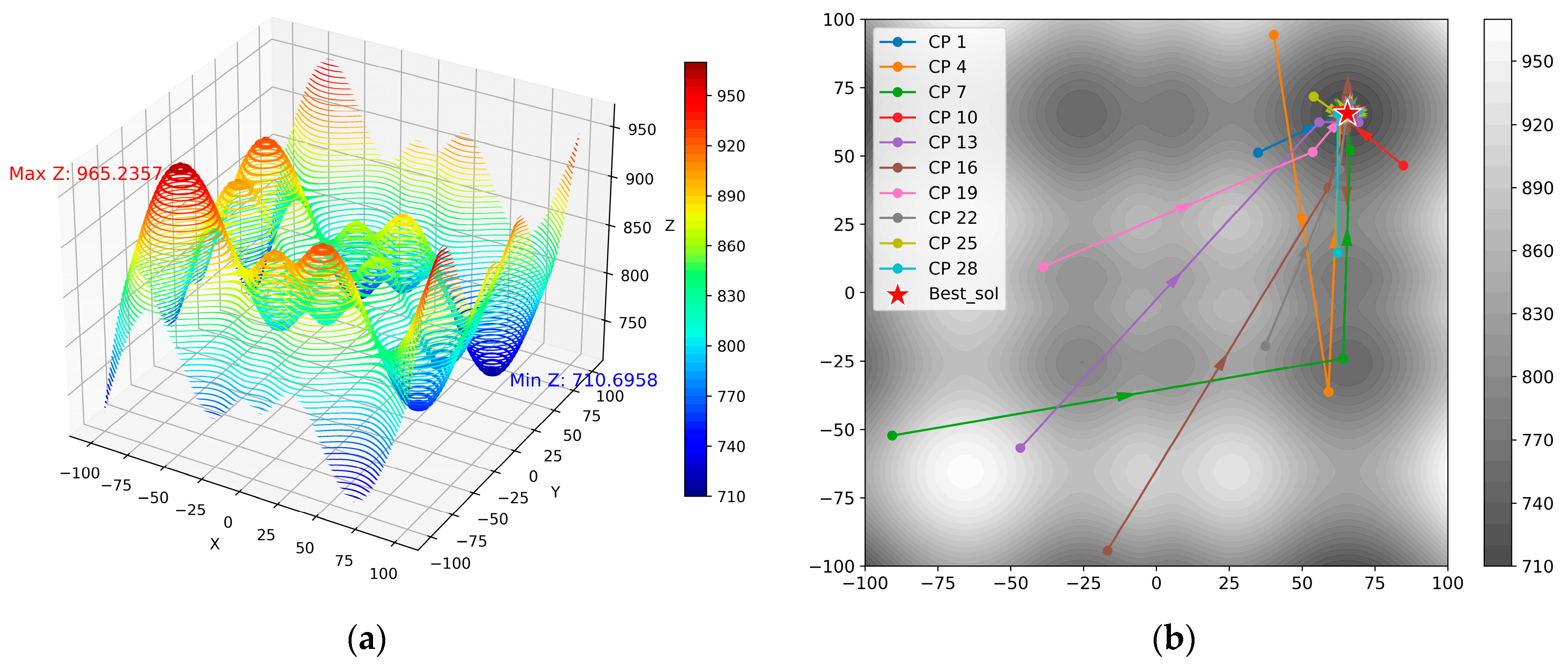
2.2.1. Crested Porcupine Optimizer

Stochastic optimization algorithms are widely used in machine learning to improve the robustness of models. Recently, meta-inspired optimization algorithms have gained the attention of researchers and are widely used to address challenging optimization problems. Most of these algorithms are based on the principles of biology, physics, behavioral science, or group intelligence and aim to simulate various characteristics of natural systems [35]. The crested porcupine optimizer (CPO) [36] is a new representative of such algorithms. It simulates the defense strategies of crowned porcupines using four strategies, namely, visual, sound, odor, and physical attacks, which are ranked by aggressiveness. These strategies map to four defense regions in the search space, which are activated sequentially on the basis of the threat level posed by the predator. Statistical analysis of the results shows that the CPO can achieve better performance in Congress on Evolutionary Computation (known as CEC) benchmarks [37] than its competitors, such as the well-known gray wolf optimizer (GWO) [38], whale optimization algorithm (WOA) [39], and salp swarm algorithm [40], with improvement rates of up to 83% for CEC2014 and 100% for six real-world engineering problems. In this work, CPO is implemented to optimize general prediction models, and the key components are summarized as follows:

• Population and fitness initialization:

The purpose of this step is to generate an initial population of candidate solutions within the specified bounds and evaluate the fitness of each solution by using an objective function for practical problems. Typically, Equations (2) and (3) are employed.

$$X_i^j=l{b}_j+{\tau }_0·(u{b}_j-l{b}_j)$$

(2)

$$f_i=f\left(X_i\right)$$

(3)

where $X_i^j$ is the $j-th$ dimension of the $i-th$ candidate solution, ${\tau }_0$ is a random value in [0, 1], and $l{b}_j$ and $u{b}_j$ are the lower and upper bounds of the $j-th$ dimension, respectively. In addition, $f_i$ is the fitness of $X_j$.

2.

Four defensive strategies in CPO

• Exploration phase (strategies 1 and 2)

When the porcupine becomes aware of the predator, it starts flapping its spines to expand its size. The predator has two options: move towards or move away from the porcupine (the distance between them decreases or increases). Equations (4) and (5) are thereby presented on the basis of the average position of randomly selected solutions. For the second strategy, the porcupine’s voice becomes louder as the predator approaches it. Gaussian perturbations are used in Equation (6) to update positions to simulate a sound attack.

$$x_i^{j+1}=x_i^j+{\tau }_1·|2{\tau }_2·x_{CP}^j-y_i^j|$$

(4)

$$y_i^j=\left(x_i^j+x_r^j\right)/2$$

(5)

$$x_i^{j+1}=(1-U_1)·x_i^j+U_1·(y+{\tau }_3·(x_{r1}^j-x_{r2}^j\left)\right)$$

(6)

where $x_{CP}^j$ is the global best solution vector; ${\tau }_1$ is a Gaussian random variable; ${\tau }_2$ is a random value in $[0,1]$; $y_i^j$ is a vector between the current porcupine and a porcupine selected randomly from the population whose solution is $x_r^j$; and $U_1$ is a binary vector, where $x_{r1}^j$ and $x_{r2}^j$ are other randomly selected solutions.

• Exploitation phase (strategies 3 and 4)

In this phase, the porcupine first secretes a fetid odor that spreads in the region around it to prevent the predator from approaching it. To achieve this, fitness-based scaling is used for updating the positions; see Equations (7)–(10). For the final strategy, the porcupine resorts to physical attack when a predator is very close and strikes it with short, thick quills. During a physical attack, the two bodies are strongly fused, representing an inelastic collision in one dimension; see Equations (11) and (12).

$$x_i^{j+1}=(1-U_1)·x_i^j+U_1·(x_{r1}^j+S_i^j·\left(x_{r2}^j-x_{r3}^j\right)-{\tau }_4·\delta ·{\gamma }_t·S_i^j)$$

(7)

$$\delta =\left\{ \begin{array}{l}\begin{array}{cc} 1& if rand\le 0.5\end{array} \\ \begin{array}{cc}-1& Else\end{array}\end{array}\right.$$

(8)

$${\gamma }_t=2·rand·{\left(1-{\displaystyle \frac{j}{j_{max}}}\right)}^{{\displaystyle \frac{j}{j_{max}}}}$$

(9)

$$S_i^j=exp\left({\displaystyle \frac{f\left(x_i^j\right)}{{\sum }_{k=1}^{N}f\left(x_k^j\right)+\mathsf{ϵ}}}\right)$$

(10)

$$x_i^{j+1}=x_{CP}^j+\left(\alpha \left(1-{\tau }_5\right)+{\tau }_5\right)·(\delta ·x_{CP}^j-x_i^j)-{\tau }_6·\delta ·{\gamma }_t·F_i^j$$

(11)

$$F_i^j={\tau }_7·{\displaystyle \frac{S_i·\left(x_i^{j+1}-x_r^j\right)}{∆j}}$$

(12)

where $x_{r3}^j$ is another randomly selected solution; $\delta$ is a parameter used to control the search direction; ${\gamma }_t$ is a factor; $S_i^j$ is the odor diffusion factor; $f\left(x_i^j\right)$ represents the objective function value of the $i-th$ individual; $\mathsf{ϵ}$ is a small value to avoid division by zero; ${\tau }_{4,\mathrm{5,6},7}$ are random values within [0, 1]; and $\alpha$ is a factor related to convergence speed.

3.

Simple case using the CPO

Below is the presentation of a straightforward optimization task aimed at finding the minimum value of a function given by Equation (13). Given the bounds of (−100, 100) and a dimension of 2, the minimum value is 710.6958 at (64.55, 64.55), as shown in Figure 2a. Figure 2b shows the search trajectories of 10 porcupines under 100 iterations when CPO is used in this case.

$$f\left(x\right)=418.9829·d-{\sum }_{i=1}^d{x}_{i}sin\left(\sqrt{\left|x_i\right|}\right)$$

(13)

where $d$ is a natural number representing the dimension of the function.

2.2.2. Gated Recurrent Unit

Wind speed prediction is a very specific but meaningful task in time series forecasting in engineering applications. Generally, time series data differ from other types of data because of their temporal nature and ordered sequence of observations. Recurrent neural networks (RNNs) can capture temporal dependencies in data by maintaining an internal state or memory, enabling them to process time-dependent sequences. Frameworks, including gated recurrent units (GRUs) and long short-term memory (LSTM) networks, were subsequently developed to address the problem of vanishing gradients when RNNs are used. Research has indicated that the LSTM and GRU architectures achieve high accuracy in time series prediction. However, the GRU exhibits comparable or even better performance than LSTM in many tasks while requiring fewer parameters, thereby consuming fewer computational resources [41,42,43]. In this work, a GRU is employed to predict wind speed series. The general equations of a single-layer GRU cell are shown in Equations (14)–(17) and Figure 3 for illustration.

$$z_t=\sigma \left(W_z{x}_t+U_z{h}_{t-1}+b_z\right)$$

(14)

$$r_t=\sigma \left(W_r{x}_t+U_r{h}_{t-1}+b_r\right)$$

(15)

$${\tilde{h}}_t=\tanh \left(W_h{x}_t+U_h\left(r_t\odot h_{t-1}\right)+b_h\right)$$

(16)

$$h_t=(1-z_t)\odot h_{t-1}+z_t\odot {\tilde{h}}_t$$

(17)

where $x_t$ is the input at time step $t$, $h_{t-1}$ is the hidden state from step $t-1$, and $\sigma$ denotes the sigmoid activation function, where $z_t$ and $r_t$ are the update and reset gates at step $t$, respectively. In addition, ${\tilde{h}}_t$ and $h_t$ are the candidate hidden state and hidden state at step $t$, respectively; $\mathrm{t}\mathrm{a}\mathrm{n}\mathrm{h}$ denotes the hyperbolic tangent activation function; $\odot$ is the element–wire operator; $W_{z, r, h}$ and $U_{z,r,h}$ are weight matrices; and $b_{z, r, h}$ are bias vectors.

2.2.3. Interval Forecasts via Kernel Density Estimation

Extensive studies have shown the effectiveness and accuracy of neural networks in time series forecasting tasks. However, these studies generally present a deterministic point prediction for these tasks and hence cannot capture the uncertainties in measured wind speed data as well as the difference between the predicted and true values. To address this, we propose employing kernel density estimation (KDE) to obtain interval values of prediction. It contains two main steps: (i) estimate the kernel density and (ii) generate confidence intervals via bootstrap resampling.

The main challenge of using this technique is to find an optimized bandwidth for the KDE. The standard univariate KDE of a discrete sequence $D=\left\{x_1, x_2, \dots ,x_n\right\}$ from an unknown function $f\left(x\right)$ is shown in Equation (18). Notably, the asymptotic convergence of $\widehat{f}(x|D,h)$ toward the underlying $f\left(x\right)$ is significantly affected by the choice of bandwidth ($h$) rather than the kernel function ($K$).

$$\widehat{f}(x|D,h)={\displaystyle \frac{1}{nh}}{\sum }_{i=1}^{n}K\left({\displaystyle \frac{x-x_i}{h}}\right)$$

(18)

where $K$ is a kernel function satisfying $\int K\left(x\right)dx=1$ and $h$ is the bandwidth.

A plausible way to choose the bandwidth is to minimize the mean integrated square error (MISE); see Equation (19). Under an integrability assumption on $f\left(x\right)$, we can further define the asymptotic mean integrated square error (AMISE), as shown in Equation (20). Afterwards, the value of the bandwidth that minimizes the AMISE is given by Equation (21). The computationally simplest method for choosing a global bandwidth is based on replacing the unknown $R\left(f^{″}\right)$ in Equation (21) with its value for a parametric family [44]. For example, Scott’s rule [45] is widely adopted, as shown in Equation (22). Additionally, a natural extension of the standard KDE uses adaptive KDE (AKDE), which is obtained when $h$ is no longer a global constant. Considering the effectiveness and efficiency of various algorithms, an AKDE method [46] employing a localized MISE and a scaled parameter is used in this work. A simple case below presents the results of KDE using various rules for comparison, as shown in Figure 4a.

$$\begin{array}{ll}\mathrm{M}\mathrm{I}\mathrm{S}\mathrm{E}\left({\widehat{f}}_h\right)& =E\left\{\int {\left({\widehat{f}}_h\left(y\right)-f\left(y\right)\right)}^{2}dy\right\}\\ & =\int {\mathrm{B}\mathrm{i}\mathrm{a}\mathrm{s}\left({\widehat{f}}_h\left(y\right)\right)}^{2}dy+\int \mathrm{V}\mathrm{a}\mathrm{r}\left({\widehat{f}}_h\left(y\right)\right)dy\end{array}$$

(19)

where $\mathrm{B}\mathrm{i}\mathrm{a}\mathrm{s}\left({\widehat{f}}_h\left(y\right)\right)={\displaystyle \frac{h^2}{2}}{\mu }_2\left(K\right)f^{″}\left(x\right)+o\left(h^2\right)$ and $\mathrm{V}\mathrm{a}\mathrm{r}\left({\widehat{f}}_h\left(y\right)\right)={\displaystyle \frac{1}{nh}}R\left(K\right)f\left(x\right)+o\left({\displaystyle \frac{1}{nh}}\right)$ are the bias and variance operators, respectively and where ${\mu }_2\left(K\right)=\int y^{2}K\left(y\right)dy>0$ and $R\left(K\right)=\int K^2\left(y\right)dy$.

$$\mathrm{A}\mathrm{M}\mathrm{I}\mathrm{S}\mathrm{E}\left({\widehat{f}}_h\right)={\displaystyle \frac{1}{nh}}R\left(K\right)+{\displaystyle \frac{h^4}{4}}{{\mu }_2\left(K\right)}^{2}R\left(f^{″}\right)$$

(20)

$$h_{\mathrm{A}\mathrm{M}\mathrm{I}\mathrm{S}\mathrm{E}}={\left[{\displaystyle \frac{R\left(K\right)}{{{\mu }_2\left(K\right)}^{2}R\left(f^{″}\right)}}\right]}^{1/5}{n}^{-1/5}$$

(21)

$$h_{\mathrm{A}\mathrm{M}\mathrm{I}\mathrm{S}\mathrm{E}}=1.06\sigma n^{-1/5}$$

(22)

where $R\left(f^{″}\right)=\int {\left[f^{″}\left(y\right)\right]}^{2}dy$ and where $\sigma$ and $n$ are the sample standard deviation and number of points (1-dimensional), respectively. Note that a more robust estimate should consider the sample interquartile; see Ref. [47].

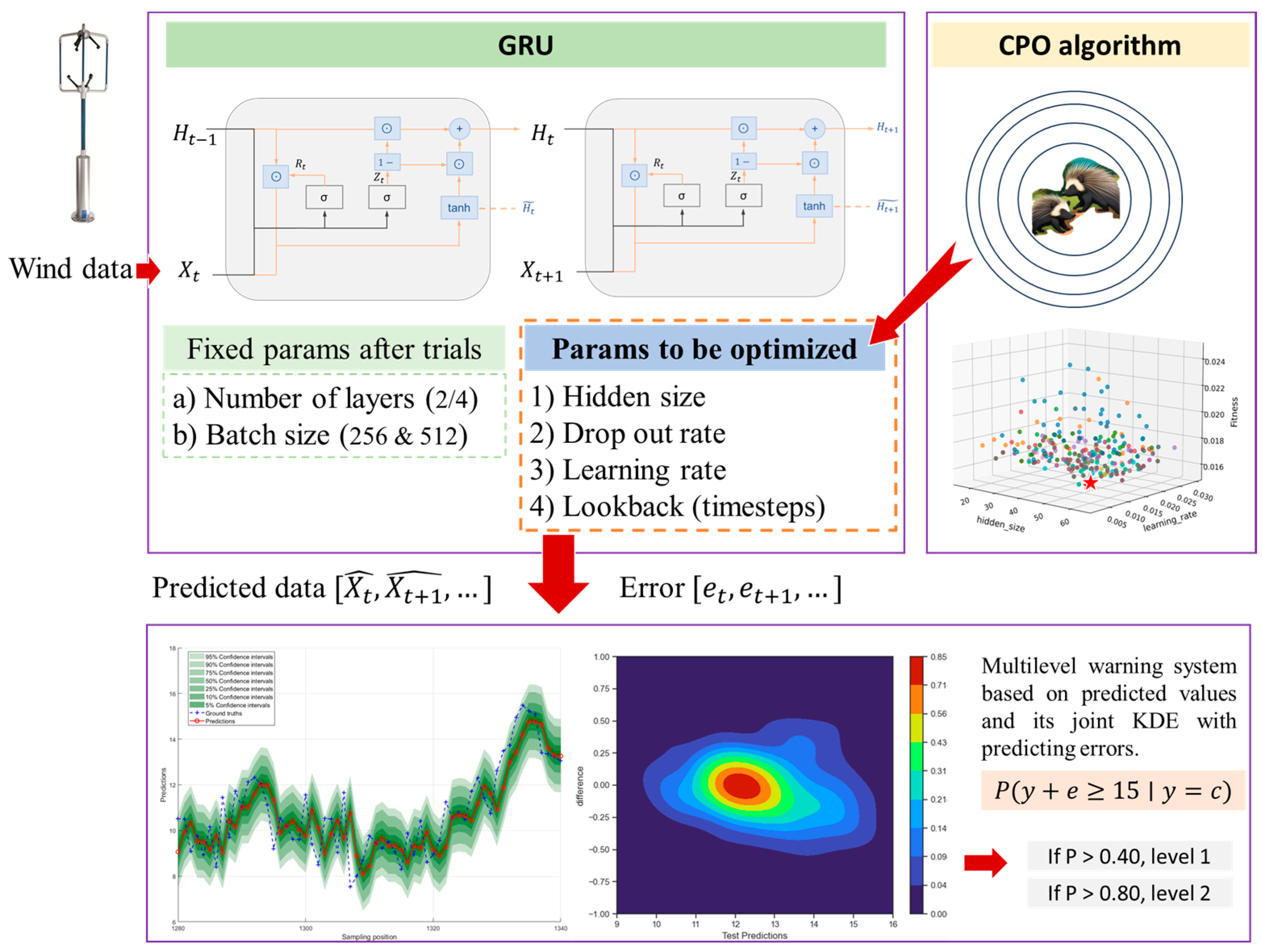
2.3. Proposed Framework

The main objective of this work is to establish a multilevel warning system by integrating various methods. By implementing prediction models, an optimization algorithm, and an adaptive estimator, we can naturally propose a framework for wind speed forecasting and establish a multilevel early warning system. The proposed framework comprises three main parts corresponding to the utilized algorithms: (i) using an optimized GRU model to predict the wind speed, (ii) performing AKDE and obtaining various confidence intervals, and finally, (iii) deciding the warning level. Figure 5 illustrates the main idea of this framework.

The warning system generates warning levels on the basis of the conditional probability of predicting values exceeding predefined thresholds. After training and optimizing the GRU, the joint KDE of the predictions and the predicted errors of the wind data can be obtained. Hence, this framework can not only predict the future wind speed $y_0$ but also evaluate the conditional probability of $P(y_0+e\ge 15\mid y=y_0)$, where $e$ is the prediction error between $y_0$ and the ground truth. Here, 15 (m/s) serves as the threshold for the speed limit of the HSR train. Two rule-of-thumb values of 0.40 and 0.80 for $P$, corresponding to two warning levels, are used. That is, the wind speed at the next step $y_0$ is first predicted by the GRU or general predictive models; then, the conditional probability $P$ is calculated and compared with threshold values of 0.40 and 0.80. Because the joint distribution is built on the basis of previous predictions and prediction errors, it is reasonable to infer that this multilevel warning method can consider the randomness of predictions and has greater credibility.

3. Results and Analysis

3.1. Performance Criteria of the Prediction Models

To objectively evaluate the prediction performance of the GRU and other RNNs used in this work, various metrics, including the root mean square error (RMSE), mean absolute error (MAE), mean absolute percentage error (MAPE), and coefficient of determination (R²), are used. The expressions of these metrics are shown in Equations (23)–(26).

$$\mathrm{R}\mathrm{M}\mathrm{S}\mathrm{E}=\sqrt{{\displaystyle \frac{1}{N}}{\sum }_{t=1}^N{(y_t-\widehat{y_t})}^2}$$

(23)

$$\mathrm{M}\mathrm{A}\mathrm{E}={\displaystyle \frac{1}{N}}{\sum }_{t=1}^N\left|\begin{array}{c}{y}_t-\widehat{y_t}\end{array}\right|$$

(24)

$$\mathrm{M}\mathrm{A}\mathrm{E}={\displaystyle \frac{1}{N}}{\sum }_{t=1}^N\left|\begin{array}{c}{y}_t-\widehat{y_t}\end{array}\right|$$

(25)

$$R^2=1-{\displaystyle \frac{{\sum }_{t=1}^N{(y_t-\widehat{y_t})}^2}{{\sum }_{t=1}^N{(y_t-\overline{y_t})}^2}}$$

(26)

where N is the length of the time series and where $y_t$ and $\widehat{y_t}$ are the actual and predicted values, respectively.

The multilevel warning system for speed limits actually serve as a binary classification model. The decision for the model is whether to implement a speed limit, whereas the real situation is whether the actual wind speed reaches 15 m/s. Hence, predictions can be categorized as true positive (TP), false positive (FP), true negative (TN), or false negative (FN). Furthermore, the true positive rate (TPR, also known as recall or sensitivity), false positive rate (FPR), and overall accuracy can be defined, as shown in

Table 3. Definitions of the prediction results of the warning systems.

Total Population = P + N		Predicted Conditions		$\mathbf{Overall} \mathbf{Accuracy}\text{:} \frac{\mathbf{T}\mathbf{P}+\mathbf{T}\mathbf{N}}{\mathbf{T}\mathbf{P}+\mathbf{T}\mathbf{N}+\mathbf{F}\mathbf{P}+\mathbf{F}\mathbf{N}}$
		Positive	Negative
Actual conditions	Positive	TP	FN	$\mathrm{T}\mathrm{P}\mathrm{R}=\mathrm{T}\mathrm{P}/(\mathrm{T}\mathrm{P}+\mathrm{F}\mathrm{N})$
	Negative	FP	TN	$\mathrm{F}\mathrm{P}\mathrm{R}=\mathrm{F}\mathrm{P}/(\mathrm{F}\mathrm{P}+\mathrm{T}\mathrm{N})$

.

3.2. Results of Optimization for RNNs

An accurate prediction of the wind speed is essential to the final decision of the warning system. To maximize the performance of RNNs, three optimization algorithms, CPO, GWO, and the WOA, are used to optimize the parameters of a two-layer GRU model. The details are as follows: (i) A sequence of length 3200 in D1-1 (see Section 2.1) is selected for optimization. (ii) The training-test split ratio, batch size, and training epochs are 80/20, 512, and 100, respectively. (iii) Four features, including the wind speed and its first-order difference, temperature, and humidity, are used to predict the next step wind speed. (iv) For a fair comparison, the population size (agent number) and iteration epoch for all algorithms are set as 30 and 20, respectively.

Table 4. Optimization using various algorithms and their performance.

Model	Parameters	Range	Initial Searching Range				Optimized Parameters
			CPO	GWO		WOA	CPO	GWO	WOA
GRU	Learning rate	0.001~0.03	0.001~0.029	0.001~0.029		0.002~0.029	0.007	0.03	0.020
	Dropout rate	0~0.3	0.002~0.285	0.010~0.291		0.003~0.289	0.002	0.082	0.211
	Hidden size	16~64	16~62	17~63		21~62	54	53	21
	Lookback	16~128	18~128	19~120		24~128	121	128	121
Model performance (on the test set of the entire D1-1)					MAPE:		1.28%	1.54%		1.52%
					MAE:		0.127	0.145		0.145
					RMSE:		0.194	0.220		0.222
					R2:		0.992	0.990		0.990

Note: The best results are in bold and underlined.

summarizes the range, initial value, and optimized selection of the parameters. Additionally, the obtained parameters are used to train and test the entire D1-1 sequence, and the model performance is shown in Table 4, where the best results are marked in bold and underline. The results of the optimization and prediction are shown in Figure 6.

As shown in Table 4 and Figure 6, all optimization algorithms have a board and satisfactory range for parameters since the initial search. According to the convergence curves in Figure 6a, the CPO obtains its optimized result at epoch 7 with an MAE loss of 0.00851, which is faster and better than those of the other two approaches. Figure 6b,c clearly show the search trends of lookback size, hidden size, and learning rate when the CPO is used. Along with Table 4, it is found that all optimization methods select a similar and relatively larger lookback size but vary in the choices of the other three parameters. For example, the CPO tends to select a lower learning rate and dropout rate and a higher hidden size, whereas the WOA performs the opposite. When the obtained parameters are applied to the full D1-1 dataset (26,280 points), as shown in Figure 6d, the performance of the GRUs is consistent with their performance on the shorter sequence (3200 points). That is, all optimized GRUs can accurately predict the wind speed, and among them, the GRU optimized by CPO performs the best predictions in terms of various metrics, including the MAPE, MAE, RMSE, and R².

3.3. Results of Various Prediction Models

To demonstrate and further compare the prediction performance of diverse statistical and RNN models, another randomly selected continuous sequence of 3200 points from D1-2 is chosen for prediction. Methods such as ARIMA, extreme learning machine (ELM [48]), RNN (GRU, LSTM, and bidirectional LSTM), and transformer [49] are employed. For machine learning methods, parameters such as the lookback size, dropout rate, learning rate, and hidden size in RNNs, as well as the hidden size in the online recurrent ELM (ORELM [50]), are optimized via the CPO. To determine the order of ARIMA, an autocorrelation function and partial autocorrelation function measures are utilized. The selected parameters and prediction results are shown in

Table 5. Parameters and prediction performance of various models.

Model	Key Parameters				Metrics
					MAPE	MAE	RMSE	R2
	Learning rate	Dropout rate	Hidden size	Lookback
GRU	0.01	0.02	63	24	2.06%	0.2108	0.1280	0.9964
LSTM	0.02	0.01	44	22	2.14%	0.2105	0.1305	0.9964
BiLSTM	0.01	0.001	57	21	2.25%	0.2187	0.1354	0.9961
ARIMA *	p	d	q	—
	1	1	3	—	2.20%	0.2112	0.1350	0.9963
	3	1	1	—	2.19%	0.2111	0.1345	0.9964
	Hidden size	Reg_lambda	Forgetting factor
ELM	30	0.001	—		2.50%	0.2195	0.1425	0.9961
ORELM	29	0.001	0.9485		3.81%	0.2142	0.3092	0.9922
	Layers	Dropout rate	No. of heads	FFN_dim
Transformer *	2	0.1	18	256	2.83%	0.2849	0.2066	0.9928

* Note: Parameters p, d, and q in ARIMA are the order of autoregressive, degree of differencing, and order of moving average, respectively; for the transformer model, FFN_dim refers to the dimension of the feedforward layer. The best results of all methods are in bold and underlined.

and Figure 7.

Frankly speaking, all applied methods show powerful applicability for the prediction of wind speed data. The prediction errors of ORELM are relatively high because the method uses an online recurrent training method, which benefits its application in real-time problems. Nevertheless, it is still more strongly affected by the choice of parameters, such as the forgetting factor; hence, the implementation of a proper optimization method is necessary. As shown in Figure 7b, the overall loss can be greatly reduced when optimized parameters are used. Moreover, it is clear that the optimized GRU model performs better than the other models do in nearly all the statistical metrics, except for the MAE. In addition, there are no distinct lag patterns in the prediction values, which is essential for the subsequent development of early warning systems. With these results, the CPO-GRU method is then applied to all the collected samples of wind speed. The prediction performance of the CPO-GRU on the collected dataset is summarized in

Table 6. Predicting results on the collected dataset via the CPO-GRU method.

Dataset	Parameters				Metric
	Learning Rate	Dropout Rate	Hidden Size	Lookback	R2	MAPE	MAE	RMSE
D1-1	0.0155	0.2320	39	26	0.9987	1.78%	0.0885	0.1416
D1-2	0.0149	0.1261	50	17	0.9913	3.84%	0.1744	0.2882
D1-3	0.0192	0.0030	45	16	0.9965	2.09%	0.1043	0.1838
D1-4	0.0128	0.0063	52	55	0.9917	1.86%	0.1192	0.3060
D2-1	0.0211	0.1958	60	92	0.9990	1.72%	0.0603	0.1045
D2-2	0.0145	0.0097	20	125	0.9931	3.58%	0.1164	0.1893
D2-3	0.0018	0.0483	60	128	0.9961	2.42%	0.1192	0.2427
D2-4	0.0299	0.0390	50	90	0.9982	0.98%	0.0666	0.1384
D2-1	0.0170	0.1583	37	17	0.9978	1.13%	0.0742	0.1421
D2-2	0.0129	0.0027	34	114	0.9687	4.34%	0.1456	0.3681
D2-3	0.0156	0.1093	33	22	0.9970	2.10%	0.0809	0.1576
D2-4	0.0141	0.0565	50	102	0.9969	0.97%	0.0988	0.1925

. Note that the agent number is 30, the optimization epoch is 20, and the training epoch is 100. As shown in Table 6, the optimized parameters generally yield good prediction performance, indicating the effectiveness of the proposed method.

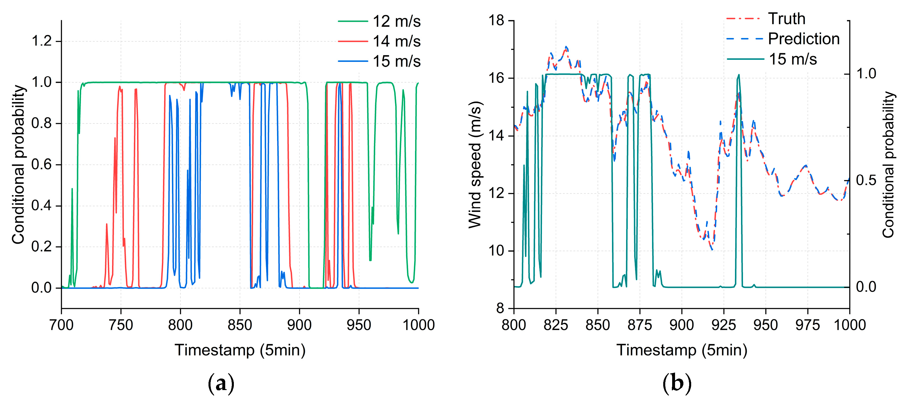
3.4. Results of Multilevel Warning

Previous analysis has demonstrated the effectiveness of the proposed prediction method. With accurate prediction values, it is then applicable to form an early warning system of the wind speed for decision making in train operations. As shown in Figure 5, a multilevel early warning system is proposed on the basis of the conditional probability of predicting values exceeding predefined thresholds. To achieve this, for each dataset (D1, D2, and D3), a joint KDE of wind speed predictions and prediction errors is first calculated from 80% of the data points (i.e., the training set) and then used for evaluating the conditional probability $P(y_0+e\ge 15\mid y=y_0)$ of the remaining 20%, where $y_0$ and $e$ are the prediction of the wind speed and the prediction error between $y_0$ and the ground truth, respectively. Notably, in practical uses, there is no need for data splitting in this phase as previous monitoring and prediction data can be used to form the joint KDE. As an example, the joint kernel density and related cumulative distribution function (CDF) of the prediction and prediction errors of D1-1 are shown in Figure 8a,b, respectively.

To demonstrate the effectiveness of the proposed multilevel warning system,

Table 7. Decisions made by various methods at points close to the critical wind speed.

Sequence ID	Values			Ideal Decision	Deterministic		Probabilistic
	True (m/s)	Pred. (m/s)	p *		Decisions	Y/N	Decision_1	Y/N	Decision_2	Y/N
3025	15.01	14.91	0.1218	1	0	N	0	N	0	N
3030	14.99	15.02	0.5695	0	1	N	1	N	0	Y
3031	14.85	15.01	0.5136	0	1	N	1	N	0	Y
3505	15.09	14.97	0.2987	1	0	N	0	N	0	N
3508	14.94	15.08	0.8010	0	1	N	1	N	1	N
3514	15.02	14.94	0.2127	1	0	N	0	N	0	N
3547	14.87	15.08	0.8010	0	1	N	1	N	1	N
3612	14.97	15.01	0.5136	0	1	N	1	N	0	Y
4893	15.03	14.93	0.1773	1	0	N	0	N	0	N
4896	14.98	15.07	0.7637	0	1	N	1	N	0	Y

Note that p * is the conditional probability of a given predicting value (Pred.) made by CPO-GRU. For decisions, 1 means the train speed should be limited, while 0 indicates the opposite. For judgements, Y means a wrong decision while N indicates the opposite. Improved results are marked with background colors.

shows the decisions at certain positions made by the deterministic and probability-based methods when predicting data. For the deterministic method, the decision of whether to limit the train speed completely depends on the accuracy of the prediction model. When the predicted speed exceeds 15 m/s, a decision to limit the train speed will be made (e.g., points 3030 and 3031); otherwise, an opposite decision will be made (e.g., points 3025 and 3505). As shown in Table 7, when the actual wind speed is close to the threshold speed, the prediction performance is never sufficient at some points. Nevertheless, when a probabilistic method is utilized, a better result can be achieved, e.g., at points 3030, 3031, 3612, and 4896. Note that the decision of level 1 is made when the conditional probability is greater than 0.4, whereas that of level 2 is 0.8.

To further compare the performance of the proposed framework, a general LSTM model is used to provide a benchmark for decision making. The LSTM model is trained for 100 epochs at a learning rate of 0.01, a dropout rate of 0.1, a hidden size of 64, and a lookback size of 64. The results are summarized in

Table 8. Result of warning decisions for the collected dataset.

Dataset	Total No. of Positive (v ≥ 15 m/s)	Total No. of TP				TPR		Overall Accuracy
		LSTM	CPO_GRU	CPO_GRU_KDE (CGK)		LSTM	CGK	LSTM	CGK
				Level 1	Level 2
D1-1	185	135	164	164	168	0.7297	0.9081	0.9903	0.9967
D1-2	3	2	2	2	2	0.6667	0.6667	0.9996	0.9996
D1-3	15	0	8	8	6	0.0000	0.5333	0.9971	0.9988
D1-4	103	82	90	90	89	0.7961	0.8738	0.9959	0.9975
D2-1	53	40	52	52	50	0.7547	0.9811	0.9975	0.9998
D2-2	0	0	0	0	0	—	—	1.0000	1.0000
D2-3	293	289	292	292	291	0.9863	0.9966	0.9965	0.9977
D2-4	73	67	61	66	68	0.9178	0.9315	0.9977	0.9990
D3-1	83	79	81	81	79	0.9518	0.9518	0.9990	0.9992
D3-2	0	0	0	0	0	—	—	1.0000	1.0000
D3-3	0	0	0	0	0	—	—	1.0000	1.0000
D3-4	437	393	408	415	410	0.8993	0.9497	0.9910	0.9926

. Here, the event is positive when the actual speed exceeds 15 m/s. The proposed CPO-GRU-KDE framework generally improves the overall accuracy, especially the TPR (see Table 3), of the prediction, which is highly significant for the presented case.

3.5. Discussions

Previous analysis has demonstrated the advances of the proposed framework. In this section, further discussions are presented to explore the reason behind these advances. In this work, to enhance the model performance, optimization algorithms are used for RNN, ELM, and transformer models. In general, using parameter optimization will not affect the properties of the model but will only find better results in the solution space. Hence, the advantage of using parametric optimization is distinct. The final choice of CPO is determined by its actual performance, as shown in Table 7. This is also the case for selecting the optimal model. As shown in Table 6, the GRU model performs the best over the other models. In addition, GRU has a simpler and more efficient structure when compared with other RNN models. Nevertheless, it is worth noting that using RNN models for time series may encounter the lagging problem—the predictive value lagging the truth value—especially when having only one training feature. Figure 9 plots the predicting results using only the previous wind speed data with MAE as the loss function. It is obvious that despite having fine metrics (R² of 0.98), the model actually provides ineffective predictions because of the occurrence of the lagging problem, which means the prediction is dominantly affected by the last one-step data. In other words, the model performance is similar to that of a naive forecast. Under this situation, the warning systems, especially those using deterministic methods, cannot perform well because the warning decisions would be lagging.

To further demonstrate the effectiveness of using probabilistic methods, two more threshold values, 12 m/s and 14 m/s, are selected to calculate the conditional probability, i.e., $P(y_0+e\ge 12\mid y=y_0$ and $P(y_0+e\ge 14\mid y=y_0$, respectively. The same joint kernel density and CDF of D1-1 dataset shown in Figure 8 are used. As plotted in Figure 10a, the conditional probability of predictions arises with the increase in threshold value. Therefore, a smaller threshold provides a broader envelope. Then, the prediction results are plotted together with their conditional probability in Figure 10b for comparison. It can be observed how the conditional probability follows the prediction values, which is achieved by the implementation of predicting error in historic data. On this basis, the final prediction values are statistically evaluated by considering both the current result of model prediction and previous database of prediction errors. This is achieved beyond the normal process of model prediction. Therefore, the subsequent decision of a warning system for the future data can be improved. As long as the model performance stays consistent, the predicting accuracy can be improved by compensating the predicting error.

4. Conclusions

In this work, we proposed a framework for wind speed prediction and related multilevel warning systems based on the combination of an optimized neural network and an adaptive kernel density estimator. The performance of various optimization algorithms, machine learning-based models, and probabilistic decision processes were evaluated. The results proved that the proposed framework performs well on the collected data. The main conclusions are as follows:

• Recurrent networks perform well in predicting wind speeds. Nevertheless, their performance can be efficiently optimized by using a proper algorithm. A comparison of various algorithms, including ARIMA, ELM, and transformer, demonstrates that the GRU performs best on the collected database.
• The results of various optimization algorithms indicate the significance of parameter optimization. The search trace of diverse parameters can provide valuable information for model selection. For example, in the present case, the lookback size greatly affects the model performance, while the model can achieve similar performance at diverse dropout rates, learning rates, or hidden sizes.
• An analysis of the prediction results indicates that the CPO-GRU model outperforms the other combinations, with metrics of 1.28%, 0.127, 0.194, and 0.992 for the MAPE, MAE, RMSE, and R², respectively, in the present case. In addition, it achieves similar and excellent performance on all collected databases.
• By using adaptive kernel estimators, the joint kernel density and cumulative distribution function of the predicted values and prediction errors can be obtained, thereby calculating the conditional probability at a given prediction of the wind speed. A comparison between the deterministic and probabilistic methods indicates that all methods yield high overall accuracy—due to the relatively large sample size—but also that the proposed framework can significantly address the TPR, which is valuable for practical decision making, especially when the predictions are near the critical value.

It is worth noting the proposed framework may encounter the lagging problem, which is a common issue in the use of RNNs. In this work, by using the L1loss function and various input features, such as temperature and humidity, the lagging problem is not obvious in the present results. Nevertheless, when the features are limited in practical use, the prediction performance should be further examined. In addition, by using joint kernel estimation and a related probabilistic approach, an advanced warning system was successfully established. The achievement of this system relies on a sufficient historic database of predictions and corresponding prediction errors. If this is not the case, the deterministic warning method, i.e., comparing the newest prediction value with the threshold value, should be used instead. Further studies should be conducted to address these issues.

References

1. Liu, D.; Wang, Q.; Zhong, M.; Lu, Z.; Wang, J.; Wang, T.; Lv, S. Effect of wind speed variation on the dynamics of a high-speed train. Veh. Syst. Dyn. 2019, 57, 247–268. [Google Scholar]
2. Liu, D.; Wang, T.; Liang, X.; Meng, S.; Zhong, M.; Lu, Z. High-speed train overturning safety under varying wind speed conditions. J. Wind Eng. Ind. Aerodyn. 2020, 198, 104111. [Google Scholar]
3. Pan, D.; Liu, H.; Li, Y. A short-term forecast method for wind speed along Golmud-Lhasa section of Qinghai-Tibet railway. China Railw. Sci. 2008, 29, 129–133. [Google Scholar]
4. Kobayashi, N.; Shimamura, M. Study of a strong wind warning system. Jr East Tech. Rev. 2003, 2, 61–65. [Google Scholar]
5. Hoppmann, U.; Koenig, S.; Tielkes, T.; Matschke, G. A short-term strong wind prediction model for railway application: Design and verification. J. Wind Eng. Ind. Aerodyn. 2002, 90, 1127–1134. [Google Scholar]
6. Jing, H.; Zhong, R.; He, X.; Wang, H. Multi-Level Early Warning Method for Gale Based on LSTM-GMM Model. China Railw. Sci. 2023, 44, 221–228. [Google Scholar]
7. Soman, S.S.; Zareipour, H.; Malik, O.; Mandal, P. A review of wind power and wind speed forecasting methods with different time horizons. In Proceedings of the North American Power Symposium 2010, Arlington, TX, USA, 26–28 September 2010; pp. 1–8. [Google Scholar]
8. Hu, J.; Heng, J.; Wen, J.; Zhao, W. Deterministic and probabilistic wind speed forecasting with de-noising-reconstruction strategy and quantile regression based algorithm. Renew. Energy 2020, 162, 1208–1226. [Google Scholar]
9. Jung, J.; Broadwater, R.P. Current status and future advances for wind speed and power forecasting. Renew. Sustain. Energy Rev. 2014, 31, 762–777. [Google Scholar]
10. Kavasseri, R.G.; Seetharaman, K. Day-ahead wind speed forecasting using f-ARIMA models. Renew. Energy 2009, 34, 1388–1393. [Google Scholar]
11. Maatallah, O.A.; Achuthan, A.; Janoyan, K.; Marzocca, P. Recursive wind speed forecasting based on Hammerstein Auto-Regressive model. Appl. Energy 2015, 145, 191–197. [Google Scholar]
12. Liu, H.; Mi, X.; Li, Y. Smart multi-step deep learning model for wind speed forecasting based on variational mode decomposition, singular spectrum analysis, LSTM network and ELM. Energy Convers. Manag. 2018, 159, 54–64. [Google Scholar]
13. Cassola, F.; Burlando, M. Wind speed and wind energy forecast through Kalman filtering of Numerical Weather Prediction model output. Appl. Energy 2012, 99, 154–166. [Google Scholar]
14. Song, J.; Wang, J.; Lu, H. A novel combined model based on advanced optimization algorithm for short-term wind speed forecasting. Appl. Energy 2018, 215, 643–658. [Google Scholar]
15. Neshat, M.; Nezhad, M.M.; Abbasnejad, E.; Mirjalili, S.; Tjernberg, L.B.; Garcia, D.A.; Alexander, B.; Wagner, M. A deep learning-based evolutionary model for short-term wind speed forecasting: A case study of the Lillgrund offshore wind farm. Energy Convers. Manag. 2021, 236, 114002. [Google Scholar]
16. Wan, J.; Liu, J.; Ren, G.; Guo, Y.; Yu, D.; Hu, Q. Day-ahead prediction of wind speed with deep feature learning. Int. J. Pattern Recognit. Artif. Intell. 2016, 30, 1650011. [Google Scholar]
17. Zhang, W.; Wang, J.; Wang, J.; Zhao, Z.; Tian, M. Short-term wind speed forecasting based on a hybrid model. Appl. Soft Comput. 2013, 13, 3225–3233. [Google Scholar]
18. Kiplangat, D.C.; Asokan, K.; Kumar, K.S. Improved week-ahead predictions of wind speed using simple linear models with wavelet decomposition. Renew. Energy 2016, 93, 38–44. [Google Scholar]
19. Liu, H.; Tian, H.-Q.; Li, Y.-F. An EMD-recursive ARIMA method to predict wind speed for railway strong wind warning system. J. Wind Eng. Ind. Aerodyn. 2015, 141, 27–38. [Google Scholar]
20. Zhang, Y.; Zhao, Y.; Kong, C.; Chen, B. A new prediction method based on VMD-PRBF-ARMA-E model considering wind speed characteristic. Energy Convers. Manag. 2020, 203, 112254. [Google Scholar]
21. Xiao, L.; Shao, W.; Jin, F.; Wu, Z. A self-adaptive kernel extreme learning machine for short-term wind speed forecasting. Appl. Soft Comput. 2021, 99, 106917. [Google Scholar]
22. Li, L.; Chang, Y.; Tseng, M.; Liu, J.; Lim, M.K. Wind power prediction using a novel model on wavelet decomposition-support vector machines-improved atomic search algorithm. J. Clean. Prod. 2020, 270, 121817. [Google Scholar]
23. Qian, Z.; Pei, Y.; Zareipour, H.; Chen, N. A review and discussion of decomposition-based hybrid models for wind energy forecasting applications. Appl. Energy 2019, 235, 939–953. [Google Scholar]
24. Marović, I.; Sušanj, I.; Ožanić, N. Development of ANN model for wind speed prediction as a support for early warning system. Complexity 2017, 2017, 3418145. [Google Scholar]
25. Gou, H.; Chen, X.; Bao, Y. A wind hazard warning system for safe and efficient operation of high-speed trains. Autom. Constr. 2021, 132, 103952. [Google Scholar]
26. Wang, L.; Li, X.; Bai, Y. Short-term wind speed prediction using an extreme learning machine model with error correction. Energy Convers. Manag. 2018, 162, 239–250. [Google Scholar]
27. Santhosh, M.; Venkaiah, C.; Kumar, D.V. Short-term wind speed forecasting approach using ensemble empirical mode decomposition and deep Boltzmann machine. Sustain. Energy Grids Netw. 2019, 19, 100242. [Google Scholar]
28. Liu, Y.; Zhang, Z.; Huang, Y.; Zhao, W.; Dai, L. Hybrid neural network-aided strong wind speed prediction along rail network. J. Wind Eng. Ind. Aerodyn. 2024, 252, 105813. [Google Scholar]
29. Wang, L.; Guo, Y.; Fan, M.; Li, X. Wind speed prediction using measurements from neighboring locations and combining the extreme learning machine and the AdaBoost algorithm. Energy Rep. 2022, 8, 1508–1518. [Google Scholar]
30. Chen, Y.; Dong, Z.; Wang, Y.; Su, J.; Han, Z.; Zhou, D.; Zhang, K.; Zhao, Y.; Bao, Y. Short-term wind speed predicting framework based on EEMD-GA-LSTM method under large scaled wind history. Energy Convers. Manag. 2021, 227, 113559. [Google Scholar]
31. Wang, H.; Xiong, M.; Chen, H.; Liu, S. Multi-step ahead wind speed prediction based on a two-step decomposition technique and prediction model parameter optimization. Energy Rep. 2022, 8, 6086–6100. [Google Scholar]
32. Zhang, C.; Ji, C.; Hua, L.; Ma, H.; Nazir, M.S.; Peng, T. Evolutionary quantile regression gated recurrent unit network based on variational mode decomposition, improved whale optimization algorithm for probabilistic short-term wind speed prediction. Renew. Energy 2022, 197, 668–682. [Google Scholar]
33. Najibi, F.; Apostolopoulou, D.; Alonso, E. Enhanced performance Gaussian process regression for probabilistic short-term solar output forecast. Int. J. Electr. Power Energy Syst. 2021, 130, 106916. [Google Scholar]
34. WRDB: Wind Resource Database. National Renewable Energy Laboratory. Available online: https://wrdb.nrel.gov/ (accessed on 16 August 2024).
35. Kaveh, A.; Dadras, A. A novel meta-heuristic optimization algorithm: Thermal exchange optimization. Adv. Eng. Softw. 2017, 110, 69–84. [Google Scholar]
36. Abdel-Basset, M.; Mohamed, R.; Abouhawwash, M. Crested Porcupine Optimizer: A new nature-inspired metaheuristic. Knowl.-Based Syst. 2024, 284, 111257. [Google Scholar]
37. Liang, J.J.; Qu, B.Y.; Suganthan, P.N. Problem definitions and evaluation criteria for the CEC 2014 special session and competition on single objective real-parameter numerical optimization. Comput. Intell. Lab. Zhengzhou Univ. Zhengzhou China Tech. Rep. Nanyang Technol. Univ. Singap. 2013, 635, 2014. [Google Scholar]
38. Mirjalili, S.; Mirjalili, S.M.; Lewis, A. Grey wolf optimizer. Adv. Eng. Softw. 2014, 69, 46–61. [Google Scholar]
39. Mirjalili, S.; Lewis, A. The whale optimization algorithm. Adv. Eng. Softw. 2016, 95, 51–67. [Google Scholar]
40. Abualigah, L.; Shehab, M.; Alshinwan, M.; Alabool, H. Salp swarm algorithm: A comprehensive survey. Neural Comput. Appl. 2020, 32, 11195–11215. [Google Scholar]
41. Chung, J.; Gulcehre, C.; Cho, K.; Bengio, Y. Empirical evaluation of gated recurrent neural networks on sequence modeling. arXiv 2014, arXiv:1412.3555. [Google Scholar]
42. Liu, X.; Lin, Z.; Feng, Z. Short-term offshore wind speed forecast by seasonal ARIMA-A comparison against GRU and LSTM. Energy 2021, 227, 120492. [Google Scholar]
43. ArunKumar, K.; Kalaga, D.V.; Kumar, C.M.S.; Kawaji, M.; Brenza, T.M. Comparative analysis of Gated Recurrent Units (GRU), long Short-Term memory (LSTM) cells, autoregressive Integrated moving average (ARIMA), seasonal autoregressive Integrated moving average (SARIMA) for forecasting COVID-19 trends. Alex. Eng. J. 2022, 61, 7585–7603. [Google Scholar]
44. Sheather, S.J. Density estimation. Stat. Sci. 2004, 19, 588–597. [Google Scholar]
45. Scott, D.W. Multivariate Density Estimation: Theory, Practice, and Visualization; John Wiley & Sons: Hoboken, NJ, USA, 2015. [Google Scholar]
46. Shimazaki, H.; Shinomoto, S. Kernel bandwidth optimization in spike rate estimation. J. Comput. Neurosci. 2010, 29, 171–182. [Google Scholar]
47. Dhaker, H.; Ngom, P.; Mendy, P. New Approach for Bandwidth Selection in the Kernel Density Estimation Based on β-Divergence. 2016. Available online: https://hal.science/hal-01297034/file/articll.pdf (accessed on 16 August 2024).
48. Zhou, S.; Liu, X.; Liu, Q.; Wang, S.; Zhu, C.; Yin, J. Random Fourier extreme learning machine with ℓ2, 1-norm regularization. Neurocomputing 2016, 174, 143–153. [Google Scholar]
49. Wen, Q.; Zhou, T.; Zhang, C.; Chen, W.; Ma, Z.; Yan, J.; Sun, L. Transformers in time series: A survey. arXiv 2022, arXiv:2202.07125. [Google Scholar]
50. Park, J.-M.; Kim, J.-H. Online recurrent extreme learning machine and its application to time-series prediction. In Proceedings of the 2017 International Joint Conference on Neural Networks (IJCNN), Anchorage, AK, USA, 14–19 May 2017; pp. 1983–1990. [Google Scholar]
Figure 1. Distribution of the wind speed and environmental data. (a) Histogram and Weibull fitting ( k = 2.27 ,   λ = 8.94 ) of the wind speed; (b) distribution of the features and target. Note that Wind, Tem, Hum, and FD refer to the wind speed, temperature, humidity, and first difference in the wind speed, respectively.
Mathematics 12 02581 g001
Figure 2. Results of seeking the minimum value via the CPO. (a) Shape of the original function; (b) searching trajectories of the porcupines (10 out of 30).
Mathematics 12 02581 g002
Figure 3. Architecture of a single-layer GRU cell.
Mathematics 12 02581 g003
Figure 4. Results of estimating an artificial sequence via KDE and AKDE. (a) Generated sequence; (b) kernel density estimations.
Mathematics 12 02581 g004
Figure 5. Framework of the multilevel warning system based on the optimized GRU and AKDE.
Mathematics 12 02581 g005
Figure 6. Optimization results of various methods and corresponding model performances. (a) Convergence curve of optimization methods; (b) searching trace of agents in the CPO for lookback size; (c) searching trace of agents in the CPO for hidden size and learning rate; (d) comparison of true wind speeds and predictions made by the GRU with different optimized parameters.
Mathematics 12 02581 g006
Figure 7. Predictions were made via various models. (a) The ACF and PACF of the sequence; (b) searching traces of the forgetting factor in ORELM via the CPO; (c) comparison between RNNs and an ARIMA model; (d) comparison between the GRU, ELMs, and a transformer model.
Mathematics 12 02581 g007
Figure 8. The KDE of predictions and prediction errors. (a) Joint kernel density; (b) CDF.
Mathematics 12 02581 g008
Figure 9. Lagging problem when using limited features in an RNN.
Mathematics 12 02581 g009
Figure 10. A demonstration of using probabilistic approaches for the warning system. (a) Conditional probability of predictions of D1-1 under various threshold values; (b) conditional probability and predictions.
Mathematics 12 02581 g010