Optimizing Electric Vehicle (EV) Charging with Integrated Renewable Energy Sources: A Cloud-Based Forecasting Approach for Eco-Sustainability

Abstract

As electric vehicles (EVs) are becoming more common and the need for sustainable energy practices is growing, better management of EV charging station loads is a necessity. The simple act of folding renewable power from solar or wind in an EV charging system presents a huge opportunity to make them even greener as well as improve grid resiliency. This paper proposes an innovative EV charging station energy consumption forecasting approach by incorporating integrated renewable energy data. The optimization is achieved through the application of SARLDNet, which enhances predictive accuracy and reduces forecast errors, thereby allowing for more efficient energy allocation and load management in EV charging stations. The technique leverages comprehensive solar and wind energy statistics alongside detailed EV charging station utilization data collected over 3.5 years from various locations across California. To ensure data integrity, missing data were meticulously addressed, and data quality was enhanced. The Boruta approach was employed for feature selection, identifying critical predictors, and improving the dataset through feature engineering to elucidate energy consumption trends. Empirical mode decomposition (EMD) signal decomposition extracts intrinsic mode functions, revealing temporal patterns and significantly boosting forecasting accuracy. This study introduces a novel stem-auxiliary-reduction-LSTM-dense network (SARLDNet) architecture tailored for robust regression analysis. This architecture combines regularization, dense output layers, LSTM-based temporal context learning, dimensionality reduction, and early feature extraction to mitigate overfitting. The performance of SARLDNet is benchmarked against established models including LSTM, XGBoost, and ARIMA, demonstrating superior accuracy with a mean absolute percentage error (MAPE) of 7.2%, Root Mean Square Error (RMSE) of 22.3 kWh, and R² Score of 0.87. This validation of SARLDNet’s potential for real-world applications, with its enhanced predictive accuracy and reduced error rates across various EV charging stations, is a reason for optimism in the field of renewable energy and EV infrastructure planning. This study also emphasizes the role of cloud infrastructure in enabling real-time forecasting and decision support. By facilitating scalable and efficient data processing, the insights generated support informed energy management and infrastructure planning decisions under dynamic conditions, empowering the audience to adopt sustainable energy practices.

1. Introduction

Introducing electric vehicles (EVs) signifies a significant change within the automotive sector when creating reliable, long-lasting transportation solutions. This has raised increasing fears of climate change and air pollution [1]. EVs offer a promising alternative to conventional internal combustion engine (ICE) cars, which significantly negatively impact the environment. Over the years, there have been significant developments in battery technology, changes in charging infrastructure, and governmental regulations to drive societal behavior towards sustainable energy solutions [2], all of which enabled this shift toward electrification.

The exponential growth of the EV industry in recent years underscores the increasing worldwide consumer embrace and integration of electric automobiles. In 2023, the global electric car fleet surpassed 15 million vehicles, marking a significant milestone in the transition to eco-friendly transportation [3]. Several factors, such as the introduction of affordable electric automobiles by prominent manufacturers, the expansion of charging infrastructure, and the decrease in battery costs, may be responsible for the increase in the adoption of electric cars.

Although the electric vehicle industry is already booming, there are still many barriers to overcome regarding widespread adaptation and consumer acceptance of electric vehicles [4]. Consumers may feel anxious when they hear about their batteries dying before reaching a charging station. To put electric vehicle owners’ minds at ease regarding the vehicle’s range, it is necessary to set up a network of charging stations that are both widely available and easy to use. Additionally, charging technologies that are fast and novel ways to increase the vehicle distance between charges must be introduced to range out the fear phenomena.

1.1. A Cloud-Based Forecasting Approach for Eco-Sustainability

Using a cloud-based forecasting method offers major progress in improving the sustainability of electric vehicle (EV) charging infrastructure. Essential for maximizing the integration of renewable energy sources, this approach uses cloud technology to enable scalability and effective data analysis. Our forecasting method uses cloud computing to handle real-time data from many sources, including renewable energy inputs and EV charging station use patterns, allowing dynamic and adaptable models that can fairly estimate energy demand and supply.

For environmental sustainability, the cloud-based architecture has several advantages. First, it offers scalability so that the forecasting models may manage rising data quantities and increasingly difficult predicting jobs without compromising performance [5]. This capacity is vital, as the acceptance of renewable energy sources and electric vehicles is rising. Second, the real-time analysis made possible by cloud technology guarantees that our projections are prompt and sensitive to evolving circumstances, thereby improving the efficiency of energy use at charging stations [6]. Furthermore, integrating several data sources into a single forecasting model helps provide more accurate forecasts, lowering dependency on non-renewable energy and reducing carbon emissions.

Thus, in line with more general environmental objectives, the cloud-based strategy increases energy consumption forecasting accuracy and supports the sustainable use of renewable energy in EV charging [7]. This method dramatically promotes the eco-sustainability of electric vehicle infrastructure by maximizing the use of the present renewable resources and guaranteeing effective energy management.

1.2. Integrating Renewable Energy Sources into Electric Vehicle Charging Infrastructure

To address the high demand for power supply in EV charging (EVC), research institutions and energy companies are exploring solutions to reduce the local electrical network burden caused by the number of dense electric car charging stations [7]. Still, the two power sources are great together to attract charging infrastructure for electric vehicles and as a solution to the local lack of resources in the electricity grid [8].

Charging infrastructure through renewable energy sources (REnSs) started to be researched in the early 2020s after the successful implementation of electric automobiles. This article aims to develop a reliable framework for solar and wind energy charging [9,10,11]. The research seeks to install enough renewable energy and direct current (DC) charging stations for electric cars (EVs). Improving the limits of the ordinary charging infrastructure could enhance the avoidance of the initiative. Due to their potential to create harmonics, deviations, and power outages, traditional charging facilities can significantly undermine the electrical grid’s reliability [12].

In contrast, the REnS provides numerous advantages, such as a higher efficiency level, lower system cost, and ease of configuration [13]. Moreover, it needs less power conversion than facilities that depend on alternating current (AC). REnS is feasible to a remarkable extent for further extension within the energy regime and its low carbon footprint will also help offset GHG emissions.

In addition, REnS can reduce the costs for electric vehicle charging [14]. Nonetheless, translating the RCI into action is fraught with significant obstacles due to variables surrounding the operation of wind (REnS-disruption in weather channel), solar concentrators, and PV power plants. At the same time, an hourly variation of cloud cover from forecast data influences a meteorologically based estimation. Moreover, the charging characteristics of electric vehicles that include features such as starting state-of-charge (SOC), battery size, number and type of vehicles involved in each query group interval, duration of time intervals for quire groups, or any minimum activity allowed between two queries, etc., pose another set of diverse challenges. By taking advantage of technological advancements such as AI, IoT, and cloud computing, The demand for intelligent and networked advanced charging systems is rapidly increasing [15].

These solutions aim to improve the charging process by making it more efficient and enhancing user experience. The intelligent, networked charging infrastructure facilitates real-time monitoring of down-charges and dynamic load management, while predictive analytics can improve energy optimization. A predictive model approach combined with data-driven analysis allows automated, optimized charging schedules that hand the control back to the individual, saving on energy costs and maximizing renewable energy utilization. Furthermore, the rise of shared and autonomous (SAE levels 4 and 5) transportation is reshaping mobility in a way that requires the development/deployment of next-generation charging infrastructure for EVs deployed as robo/cyber-taxis. The integration of wireless charging technologies with vehicle-to-grid (V2G) communication systems is becoming increasingly important due to the rising use of self-driving cars [16].

The effective operation of EV charging stations depends on accurate forecasts, particularly for significant fluctuations in energy consumption. Good forecasting helps allocate and schedule renewable energy supplies better, lowering dependency on non-renewable sources and running costs. In areas where solar energy is the leading renewable source, this method is critical as it best uses the already existing solar electricity during times of maximum output.

1.3. Contributions

This is important for creating easy and efficient charging processes to service autonomous EV fleets. Therefore, we need to find ways to integrate REnSs with electric vehicles (via smart charging solutions). Hence, we can speed up the process of decarbonizing the transportation sector. The original components of the analysis are as follows:

• Introduced a new approach called Temporal Contextual Imputation (TCI) to deal with missing data in temporal sequences while keeping time dynamics intact and ensuring that EVC station load forecasts are consistent in context.
• Integration of renewable energy and weather data: incorporated solar and wind energy statistics into EVC station energy consumption forecasting across multiple California locations.
• Enhanced EMD signal decomposition: implemented empirical mode decomposition (EMD) to extract temporal patterns from EVC station load data, enhancing forecasting accuracy.
• Feature engineering: utilized the Boruta method for feature selection and engineering, creating new features to capture inherent data relationships effectively.
• SARLDNet architecture development: introduced SARLDNet (stem-auxiliary-reduction-LSTM-dense network), a novel deep learning architecture optimized for robust EVC station load forecasting.
• Execution efficiency: achieved efficient execution time and low complexity with SARLDNet, contributing to accurate and scalable forecasting solutions.

1.4. Organization of Paper

The sections that follow contain the remaining content of the article. The second section presents existing research/studies in this specific area. The third part goes into detail about the approach suggested for this investigation. In the last section, some of the results of this study and benchmarks are described and simulated.

2. Related Work

Significant studies have been conducted on electric vehicles, mainly modeling the demand for charging in an EV-ubiquitous scenario and managing the energy requirements of numerous load aggregations. Various innovative approaches, such as algorithmic optimization, fuzzy logic, and machine learning, have been explored to tackle these challenges. This section delves into the latest research that expands our understanding and enhances the EV demand load, energy management, and charging station load forecast. The practical applications of the research are equally inspiring. For instance, the Bayesian extreme learning machine was employed for SOC modeling in hybrid electric vehicles [17], a crucial step in effectively managing energy requirements in electric cars. Furthermore, researchers in [18] used machine learning to evaluate energy consumption and electric vehicle patterns accurately, a calculation vital for creating reliable energy management systems for EV charging stations. At Los Angeles’s University of California, electric car charging stations implement electricity consumption implementation forecasts using phone and mobility data [19]. Here is a way to forecast energy use by fusing different data sources. In recent research [20,21], the goal of multi-mode switching logic control for PHEVs (Plugin Hybrid Electric Vehicles) realized energy need prediction and fuel efficiency improvement over certain tracks. A machine learning method was developed to predict the capacity needs of charging stations. This has the advantage of helping to organize and streamline the infrastructure needed for charging electric cars. In [22], statistical attributes of the EV data were collected and fed to supervised learning models for energy consumption estimations, which allowed for making more accurate predictions of electricity load. The author of [23] proposed a transfer learning approach to develop prediction models, drawing on data from multiple EV makes and models. It makes energy usage forecasts more accurate and flexible. The ability to improve energy utilization using more accurate forecasts has been shown in [24], where short-term predictions were incorporated into an energy management strategy for hybrid electric vehicles. The author of [25] proposed forecasting methods for predicting available capacity and EV energy consumption by applying the parallel gradient boost decision tree model. The study [24] demonstrated that more precise forecasts could improve energy efficiency through short-term predictions when integrated into a hybrid electric vehicle operating strategy. A set of forecasting models was introduced in [25] to predict schedulable capacity and EV energy consumption using a concurrent gradient boosting decision tree approach. The research paper [26] is a testament to the potential of machine learning in revolutionizing the future of electric vehicles. By accurately predicting the power requirements of electric vehicles (EVs), these advanced machine learning algorithms are paving the way for more efficient and sustainable predictive modeling.

Scheduled capacity and EV energy consumption prediction models by parallel gradient boost decision tree are introduced in [25]. Another study [24] showed that higher precision forecasts can improve energy efficiency by using real-time short-term predictions in the context of an online optimal energy management strategy for a hybrid electric vehicle.

The research paper [25] proposed prediction models to predict schedulable capacity and EV energy consumption by using a parallel gradient boosting decision tree method. The paper highlighted that advanced machine learning technology can accurately predict energy use. In [26], machine learning algorithms are utilized to predict energy consumption for electric vehicles (EVs) by representing the state of the art of commonsense-based autonomy. These methods have completely redefined predictive modeling.

Considering the increasing number of electric cars, a technique was developed in the research by [27] to predict long-term energy use. Several aspects were employed in this approach to improve the forecast accuracy. In [28], the efficacy of an extreme learning machine algorithm in evaluating EV energy demand and enhancing energy utilization EVs was illustrated. This endeavor exemplified the practicality of machine learning methods in improving energy efficiency.

Using imprecise logic, the researchers assigned the energy in an ESS in [29]. The imprecise controller calculates the filter cutoff frequency based on the current state of charge (SoC) of the ESS. To ascertain the electrical capacity accessible in a V2G parking area, an analytical model is introduced in [30]. The model considers the uncertainty surrounding the quantity of energy and electricity that any electric car can generate. The fuzzy controller described in [31] modulates the battery power in response to the disparity between power and state of charge (SoC). The energy distribution is optimized when the unit with the greatest SoC injects tremendous energy and consumes less.

Effective energy management depends on the battery energy storage system (BESS) used in electric cars (EVs) having the best capacity, as [32,33] focus on determining. The work reported in reference [34] successfully created and validated an automated learning system. This automation showed how two wind power sources and two battery swap stations for electric vehicles (EVs) interact in a mixed-modal setting.

Energy storage systems (ESSs) have been employed with various filters, including first-order, low-pass, and ramp-rate (R-R) filters, to reduce fluctuations. The authors of [35,36,37], have provided an abundance of information on design techniques. The ramp-rate method is a practicable solution that restricts the rate at which power can either increase or diminish to stabilize power. According to [38], dynamically altering the rising rate in real time to take into account the changing conditions of renewable sources and electric vehicles (EVs) increased the method’s effectiveness.

The connection power estimation for an energy storage system for batteries (BESS) was enhanced by applying fuzzy logic techniques in [39]. Predictive control strategies were emphasized in the research due to their advantages. The authors of [39] employed two high-frequency attenuation filters to determine the powers connected with a (BOSS). Utilizing a fuzzy controller that adjusted the cutoff frequency of the filters by the BESS’s SoC, the precision of energy management was further enhanced.

In [40], the author presents a framework for the predictive control of artificial intelligence models. AI can optimize energy consumption by focusing on the energy management structure of a series of hybrid electric vehicles, as demonstrated by this framework. A system was proposed in [41] to anticipate electric cars’ future velocity profiles and energy consumption by combining deterministic and stochastic components. This method considers the characteristics of the drivers, the route information, and the ambiguity of the traffic flow. The issue of EV charging forecasting was addressed in [42] by combining a temporal encoder–decoder LSTM and a temporal LSTM. The research indicates that deep learning techniques were effective in resolving this issue.

Federated learning was employed by [43] to choose a semi-decentralized robust network and certified local models for power management and EV charging consumption prediction. The possibilities of collaborative learning paradigms are highlighted in this study. In concert, these works advance the fields of energy consumption management at charging stations and demand forecasts for electric vehicle charging. Applying machine learning, fuzzy logic, and optimization algorithms offers solutions to the issues presented by the increasing popularity of electric cars and the rising dependence on renewable energy sources.

Table 1. Summary of related works and their challenges.

Ref.	Method Used	Problem Identified	Limitations
[17]	Bayesian extreme learning machine	Uncertainty in EV charging consumption	Limited to SOC prediction, may not consider all factors
[18]	Machine learning algorithms	Estimation of energy consumption in EVs	Dependency on quality and quantity of training data
[19]	Algorithm utilizing cell phone data	Predicting energy consumption at EV charging	Reliance on availability and reliability of cell phone data
[20]	Strategy for multi-mode toggle logic control	Enhancing energy forecasting and fuel economy	May not adapt well to dynamic driving conditions
[21]	Machine learning for capacity prediction	Planning and optimizing charging station infrastructure	Dependency on accurate data for capacity prediction
[22]	Statistical features extraction and supervised learning	Supervised learning for energy consumption prediction	Reliance on availability of comprehensive EV data
[23]	Transfer learning algorithms	Transfer learning for prediction model construction	Dependency on availability of sufficient transfer data
[24]	Integration of prediction models with energy management strategies	Integration of short-term predictions into energy management	Complexity in integrating prediction models with management systems
[25]	Decision tree algorithm with parallel gradient boosting	Energy demand and schedulable capacity forecasting	Complexity in implementing and training boosting algorithms
[26]	Advanced machine learning techniques	Using cutting-edge machine learning techniques, new methods	Potential overfitting and complexity in model interpretation
[27]	Combination of attributes for prediction	Long-term forecasting approach for energy consumption	Dependency on accurate historical data for forecasting
[28]	Extreme learning machine algorithm	Optimal energy management using extreme learning machine	Sensitivity to input parameters and training data quality
[29]	Fuzzy logic algorithms	Energy storage system (ESS) fuzzy logic algorithm	Complexity in tuning fuzzy controller parameters
[30]	Analytical model for V2G parking lot	Power capacity of the V2G parking lot computed	Assumption-based model, may not accurately reflect real-world conditions
[31]	Filtering techniques using ESS for power compensation	Attenuation of power fluctuations using ESS	Design limitations of filtering techniques
[32]	Ramp-rate technique for power smoothing	Limiting power rate changes for smoothing	Challenge in selecting appropriate ramp-rate parameters
[33]	Use of fuzzy logic for designation of reference powers	Installation of BESS’s relevant authorities	Complexity in fuzzy controller tuning and system integration
[34]	Development of learning action automaton	Implementation and validation of learning action automaton	Complexity in system validation and real-world implementation
[35]	Utilization of R-R filters for fluctuation attenuation	Fluctuation attenuation using ESS and R-R filters	Design limitations and challenges in selecting filter parameters
[36]	Adjustment of ramp-rate in real time for power stabilization	Real-time adjustment of ramp-rate for power stabilization	Complexity in real-time control and coordination
[37]	Fuzzy logic algorithm for designation of reference powers	Designation of reference powers for a BESS	Complexity in fuzzy controller tuning and system integration
[38]	High-frequency attenuation filters with fuzzy controller	Power calculation using BESS and high-frequency attenuation filters	Complexity in fuzzy controller tuning and system integration
[39]	Probabilistic prediction models for energy consumption prediction	Comparison of probabilistic and deterministic prediction models	Complexity in model training and interpretation
[40]	Usage of historical charging data for EV session prediction	Prediction of EV session duration and energy consumption	Dependency on historical data quality and availability
[41]	Long short-term memory and ARIMA models for charging loads	Forecasting EV charging station usage using time series data	Complexity in model selection and parameter tuning
[42]	BP neural network for driving condition prediction	Driving conditions prediction model for parallel hybrid electric vehicles	Dependency on accurate driving condition data and model tuning
[43]	A data-driven methodology for predicting the energy consumption of large-scale charging	Prediction of large-scale charging energy demands	Complexity in model training and scalability
Ours	Temporal Contextual Imputation (TCI), Integration of Renewable Energy and Weather Data, Enhanced EMD Signal Decomposition, Feature Engineering, SARLDNet Architecture Development, and Execution Efficiency.	Addressed limitations with innovative methods for handling missing data, integrating renewable energy data, enhancing signal decomposition, advanced feature engineering, novel deep learning architecture, and efficient execution, improving accuracy and scalability in EV charging station load forecasting.	Overcame traditional challenges with comprehensive methods integrating novel data handling, improving accuracy and scalability.

outlines the current literature on the subject.

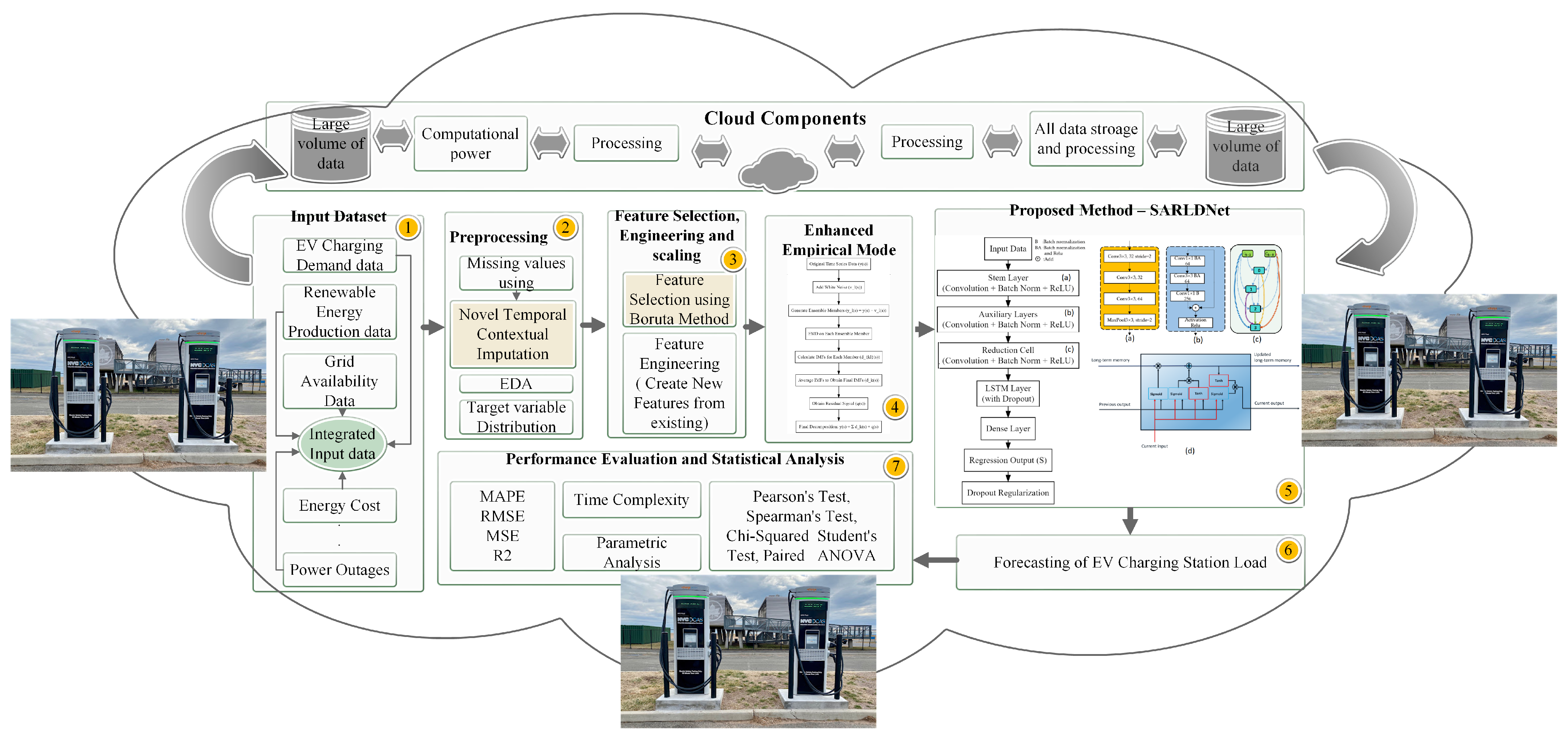
3. Proposed Methodology

The proposed framework evaluates the need for EV charging stations by combining renewable energy statistics with other pertinent data in our dataset. This dataset was collected from Kaggle data from several sources over 3.5 years, including solar energy, wind patterns, and charging station use from four particular California locations. Then, this information was aggregated into a single dataset to provide the basis for our analysis. A cloud-based forecasting method was used to effectively handle and examine this large dataset. This method uses the cloud’s scalability and computing capability to manage vast data and execute real-time processing. Cloud-based technology improves the accuracy and timeliness of our predictions by combining data from many sources, including renewable energy inputs. This is essential for the best utilization of renewable energy in EV charging stations. Following data aggregation, we used comprehensive preprocessing techniques, employing a new approach to handle missing values. After that, feature selection techniques, most notably the Boruta method, were used to find essential dataset traits. Following this step was feature development, in which we developed five fresh features from the current ones to increase the capacity of the model to grasp underlying relationships and data patterns. Augmented EMD broke down the time series data into intrinsic mode functions (IMFs), improving prediction accuracy. This breakdown helped us uncover latent trends and patterns, improving the model’s capacity to provide exact forecasts. After feature engineering and preprocessing, the novel SARLDNet model was used for regression analysis. This approach was primarily meant to estimate the demand at EV charging stations. Incorporating renewable energy sources guaranteed the reliability of the load using quick charging capabilities and resolved power system uncertainties or contingencies. This method finally increased the efficiency and efficacy of EV charging activities by providing timely and precise estimates.

Figure 1 depicts a graphic representation of the suggested framework. The following parts will discuss the specific information in the previously described model.

3.1. Impact of Key Features

Table 2. List of sample of original and derived features and descriptions.

Feature Type	Feature Name	Description
Original	Date	The specific date of the recorded data.
Original	Time	The hour of the day the data was recorded.
Original	EV Charging Demand (kW)	The amount of electricity (in kilowatts) demanded by electric vehicles for charging each hour.
Original	Solar Energy Production (kW)	The amount of electricity (in kilowatts) produced from solar energy sources during each hour.
Original	Wind Energy Production (kW)	The amount of electricity (in kilowatts) produced from wind energy sources during each hour.
Original	Electricity Price ($/kWh)	The price of electricity per kilowatt-hour.
Original	Grid Availability	Indicates whether the grid was available (“Available”) or not (”Unavailable“) during each hour.
Original	Weather Conditions	Describes the weather during each hour, with values such as “Clear”, “Cloudy”, “Rainy”, etc.
Original	Battery Storage (kWh)	The amount of electricity stored in batteries during each hour.
Original	Charging Station Capacity (kW)	The maximum capacity of the charging stations in kilowatts.
Original	EV Charging Efficiency (%)	The efficiency of the EV charging process, expressed as a percentage.
Original	Number of EVs Charging	The number of electric vehicles charging each hour.
Original	Peak Demand (kW)	The peak electricity demand during each hour.
Original	Renewable Energy Usage (%)	The percentage of energy used from renewable sources.
Original	Grid Stability Index	An index indicates the grid’s stability, with higher values indicating greater stability.
Original	Carbon Emissions (kgCO2/kWh)	The amount of carbon emissions produced per kilowatt-hour of electricity.
Original	Power Outages (hours)	The duration of power outages during each hour.
Original	Energy Savings ($)	The amount of money saved through energy efficiencies during each hour.
Derived	Total REn Production (kW)	The sum of solar and wind energy production.
Derived	Effective Charging Capacity (kW)	The product of charging station capacity and EV charging efficiency.
Derived	Adjusted Charging consumption (kW)	The EV charging demand adjusted by renewable energy usage.
Derived	Net Energy Cost ($)	The product of EV charging demand and electricity price.
Derived	Carbon Footprint Reduction (kgCO2)	The reduction in carbon emissions due to renewable energy usage.
Derived	Renewable Energy Efficiency	The efficiency of utilizing renewable energy for charging electric vehicles.

summarizes various important elements in our forecasting system. Every one of these characteristics significantly improves the demand forecast accuracy for electric vehicle charging stations:

• Weather conditions: Temperature, humidity, and wind speed are crucial factors that directly influence renewable energy production. For instance, solar energy production mainly depends on sunlight, which is subject to atmospheric influences. By incorporating these features, our model can more precisely account for variations in renewable energy supply.
• Time of day and day of week: These attributes facilitate the identification of daily and weekly fluctuations in demand for electric vehicle charging. Understanding peak utilization times facilitates better demand forecasting and resource allocation.
• Historical charging patterns: Analyzing historical charging patterns offers valuable insights into utilization trends and enhances the accuracy of future demand predictions.

Our method guarantees that the model is more capable of managing the diverse factors that affect the availability of renewable energy and the demand for EV charging by integrating these features.

3.2. Grid Stability Index Calculation

Evaluating the dependability of the electricity grid concerning EV charging stations depends mainly on the grid stability index. This index uses several elements to guarantee the stability of energy demand and supply.

First, Load Variability measures variations in EV charging station power demand. Since these variations affect general grid stability, they are crucial. High unpredictability may make it difficult for the grid to provide a constant supply, particularly in times of great demand.

Second, renewable energy integration evaluates the grid effect of including solar and wind energy sources. Since renewable energy sources are, by nature, intermittent, their fluctuation has to be taken into account if one is to assess their impact on grid stability fairly.

Stability measures reflecting both voltage stability and power demand help one calculate the grid stability index. This computation uses the formula

$$\mathrm{Grid}\mathrm{Stability}\mathrm{Index}={\displaystyle \frac{1}{N}}\sum _{i=1}^N\left({\displaystyle \frac{P_i-\overline{P}}{{\sigma }_P}}\right)+\left({\displaystyle \frac{V_i-\overline{V}}{{\sigma }_V}}\right)$$

(1)

$\overline{P}$ is the average power demand; $P_i$ is the power demand at time i; ${\sigma }_P$ is the standard deviation of the power demand. Comparably, $V_i$ is the voltage at time i, $\overline{V}$ is the average voltage, and ${\sigma }_V$ is the standard deviation of voltage. And, last, N indicates the total count of observations used in the computation.

This index guarantees a constant and dependable energy supply by helping to assess how effectively the power grid can manage the dynamic character of EV charging demand and the integration of renewable energy sources.

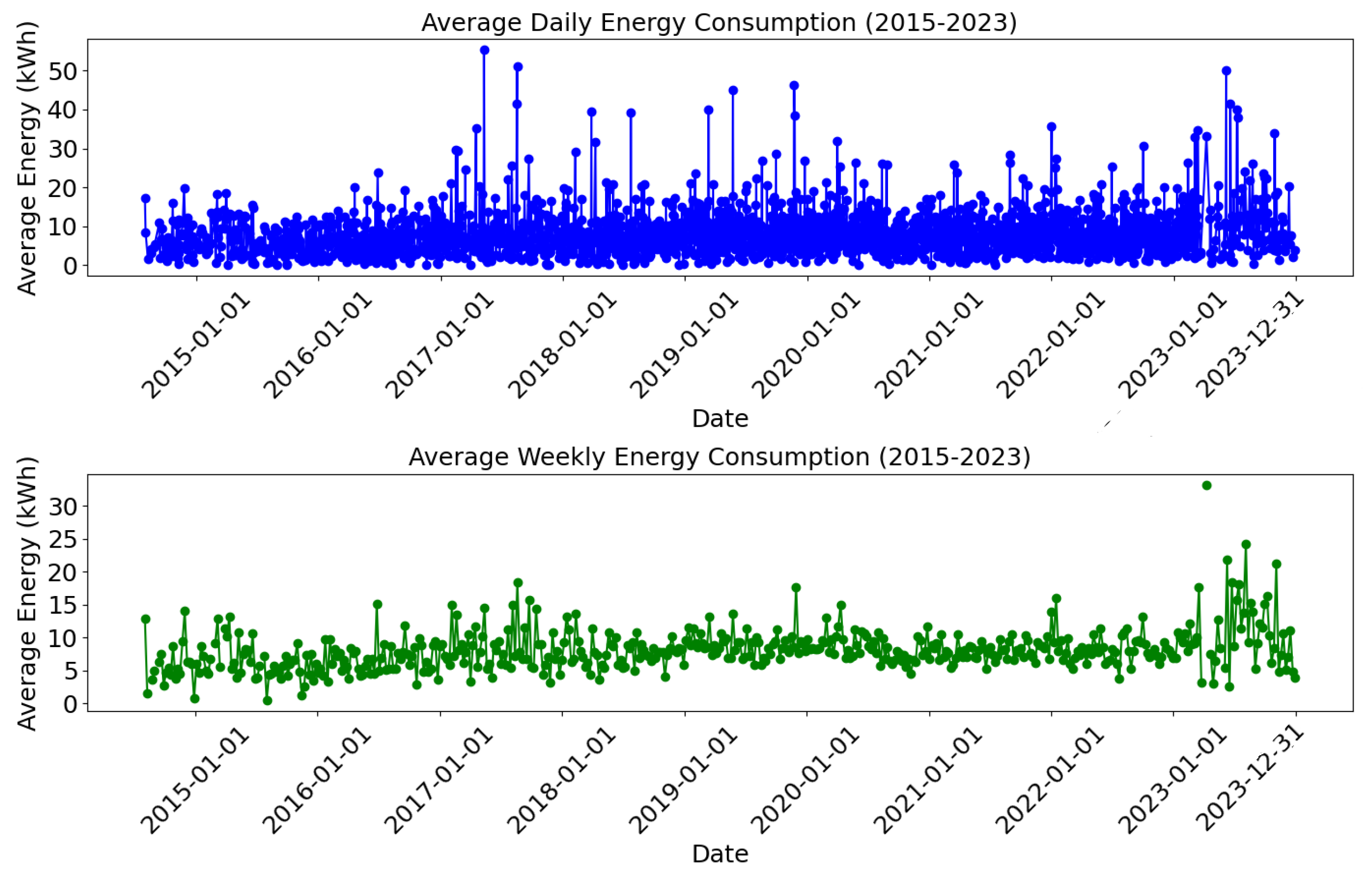
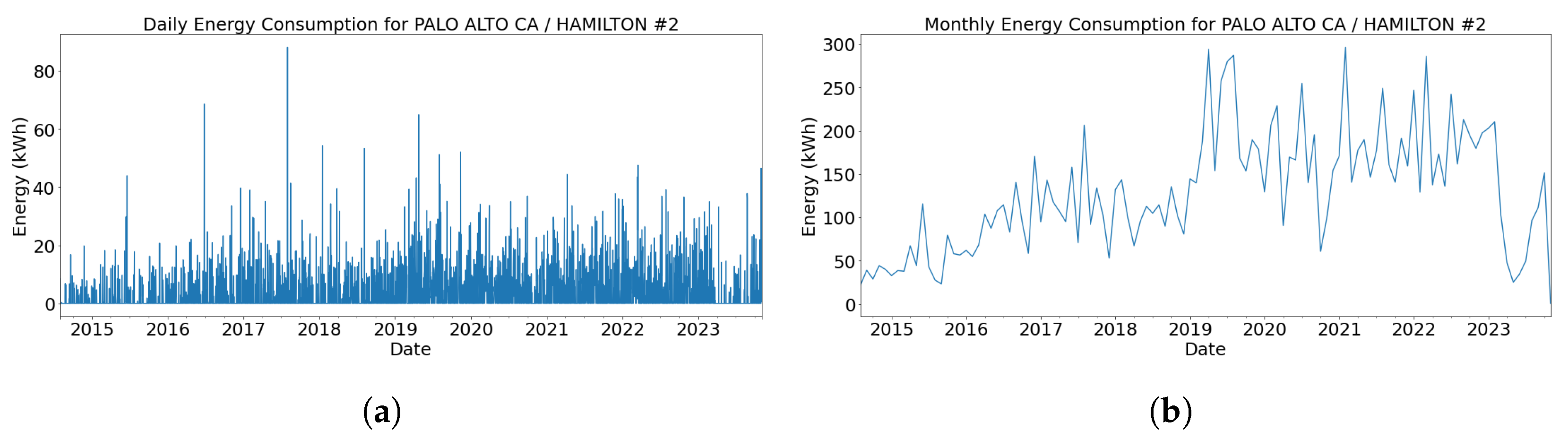
3.3. Dataset Description

This work uses data from Kaggle that combine load data from EV charging stations with renewable solar and wind energy sources [44]. This simple dataset has a list of 35 EV charging stations in California, along with the record from the year 2014 to the year 2023. Benchmark: It has 51 features and provides a complex dataset for experimentation consisting of binary data with multiple levels/deep nesting. Data for each charging station are recorded, making it easier to explore the modeling and development of how REnS data can be combined with aggregated EV consumption per charge on a site level. It exposes many aspects of energy generation, use, and environmental improvements, including original and derived features. In the dataset, PALO ALTO CA/HAMILTON 1 corresponds to Charging Station A, PALO ALTO CA/HAMILTON 2 corresponds to Charging Station B, PALO ALTO CA/MPL 6 corresponds to Charging Station C, and PALO ALTO CA/WEBSTER 1 corresponds to Charging Station D.

3.3.1. Derived Features

Total REn Production (kW): The Total REn Production (kW) feature is built by adding solar and wind energy production values. This summarizes how much renewable energy can be accessed for EV charging. It helps quantify the total renewable contribution, allows sustainable charging actions to be tracked, and depreciates dependency on non-renewable energy sources.

$$\mathrm{Total}\mathrm{REn}\mathrm{Production}\left(\mathrm{kW}\right)=\mathrm{Solar}\mathrm{Energy}\mathrm{Production}\left(\mathrm{kW}\right)+\mathrm{Wind}\mathrm{Energy}\mathrm{Production}\left(\mathrm{kW}\right)$$

(2)

Higher values of Total REn Production indicate greater availability of renewable energy, reducing the load on EV charging stations and promoting environmentally friendly charging practices.

Effective Charging Capacity (kW): The Effective Charging Capacity (kW) feature adjusts the maximum charging station capacity based on the efficiency of the EV charging process. Considering efficiency losses, it represents the power available for charging EVs. This metric aids in accurately assessing the charging infrastructure’s capability, accounting for efficiency losses during the charging process. It provides insights into the actual usable energy for charging EVs, aiding in optimizing charging schedules and resource allocation to meet demand while minimizing energy waste.

$$\mathrm{Effective}\mathrm{Charging}\mathrm{Capacity}\left(\mathrm{kW}\right)=\mathrm{Charging}\mathrm{Station}\mathrm{Capacity}\left(\mathrm{kW}\right)\times \left({\displaystyle \frac{\mathrm{EV}\mathrm{Charging}\mathrm{Efficiency}(\%)}{100}}\right)$$

(3)

Adequate Charging Capacity provides insights into the actual usable energy for charging EVs, optimizing charging schedules and resource allocation to meet demand while minimizing energy waste.

Adjusted Charging consumption (kW): The Adjusted Charging consumption (kW) element accounts for the extent to which EV charging demand can be served by renewable energy; it scales forward the total amount of storage power used based on the fraction available from renewables. It is a sustainability and environmentally friendly metric considering the share of renewable energy integration in EV charging demand.

$$\mathrm{Adjusted}\mathrm{Charging}\mathrm{Demand}\left(\mathrm{kW}\right)=\mathrm{EV}\mathrm{Charging}\mathrm{Demand}\left(\mathrm{kW}\right)\times \left({\displaystyle \frac{\mathrm{Renewable}\mathrm{Energy}\mathrm{Usage}(\%)}{100}}\right)$$

(4)

Higher values of Adjusted Charging Demand indicate increased utilization of renewable energy for EV charging, reducing the load on charging stations and promoting sustainable charging practices.

Net Energy Cost ($): The Net Energy Cost ($) feature represents the total cost incurred for supplying electricity to charge EVs, considering the EV charging demand and electricity price. This metric quantifies the financial expenses associated with providing electricity for EV charging, aiding in cost-benefit analysis and financial planning for charging infrastructure.

$$\mathrm{Net}\mathrm{Energy}\mathrm{Cos}\mathrm{t}(\$)=\mathrm{EV}\mathrm{Charging}\mathrm{Demand}\left(\mathrm{kW}\right)\times \mathrm{Electricity}\mathrm{Price}(\$/\mathrm{kWh})$$

(5)

Net Energy Cost highlights the financial implications of EV charging, emphasizing the importance of optimizing charging strategies to minimize costs and maximize cost-efficiency.

Carbon Footprint Reduction (kgCO₂) When comparing renewable energy to traditional power sources for charging electric vehicles, the Carbon Footprint Reduction (kgCO₂) metric provides a numerical value for the amount of carbon emissions cut. This statistic evaluates the environmental advantages of charging electric vehicles using renewable energy, which may help with plans to reduce carbon emissions.

$$\begin{array}{c}\hfill \mathrm{Carbon}\mathrm{Footprint}\mathrm{Reduction}\left({\mathrm{kgCO}}_2\right)=\mathrm{EV}\mathrm{Charging}\mathrm{Demand}\left(\mathrm{kW}\right)\times \mathrm{Carbon}\mathrm{Emissions}({\mathrm{kgCO}}_2/\mathrm{kWh})\times \\ \hfill \left(1-{\displaystyle \frac{\mathrm{Renewable}\mathrm{Energy}\mathrm{Usage}(\%)}{100}}\right)\end{array}$$

(6)

Higher values of carbon footprint reduction indicate more significant reductions in carbon emissions, emphasizing the role of renewable energy integration in promoting environmental sustainability.

Renewable Energy Efficiency: The Renewable Energy Efficiency feature evaluates the effectiveness of using renewable energy for charging electric vehicles by considering the ratio of total renewable energy production to adequate charging capacity. This statistic measures the effectiveness of using renewable energy to fulfill the demand for electric vehicle charging, which is a way to measure sustainability.

$$\mathrm{Renewable}\mathrm{Energy}\mathrm{Efficiency}={\displaystyle \frac{\mathrm{Total}\mathrm{REn}\mathrm{Production}\left(\mathrm{kW}\right)}{\mathrm{Effective}\mathrm{Charging}\mathrm{Capacity}\left(\mathrm{kW}\right)}}$$

(7)

Higher values of Renewable Energy Efficiency reflect more effective utilization of renewable energy for EV charging, reducing the load on charging stations and promoting sustainable transportation practices.

3.4. Missing Values Imputation Using Novel Temporal Contextual Imputation (TCI) Method

Dealing with missing data is an essential preprocessing task in guaranteeing our models’ predictive accuracy and consistency for load prediction at EV charging stations. To address this problem, we propose a new method called TCI. This method uses the temporal dependencies and contemporary relations of variables in a dataset to impute missing values, thereby preserving this information and ensuring that the filled-in dataset has similar temporality characteristics to its original features.

The TCI algorithm can be divided into three phases: temporal dependency analysis, contextual pattern identification, and contextual imputation. Each phase is performed so that the imputed values remain consistent with observed data temporal and contextual patterns, ensuring the quality of the imputations.

Temporal Dependency Analysis: In the first process of this layer, we evaluate temporal dependencies on data to detect trends and seasonality/time-based correlation patterns. This is achieved through the following processes:

• Autocorrelation analysis: we calculate each feature’s autocorrelation function (ACF) to identify temporal dependencies.
• Seasonal decomposition: using seasonal and trend segmentation using Loess (STL), we separate the time series data into three parts: seasonal, trend, and residual. The formula for the seasonal breakdown of the time series $y\left(ts\right)$ is as follows:

  $$Y\left(ts\right)=T\left(ts\right)+A\left(ts\right)+E\left(ts\right)$$

  (8)
  The trend component is denoted as $T\left(ts\right)$, the seasonal component is denoted as $A\left(ts\right)$, and the residual component is denoted as $E\left(ts\right)$.

Contextual Pattern Identification: In the second phase, we identify contextual patterns in the data that can be used to guide the imputation process. This includes the following processes:

• Feature correlation analysis: we calculate the correlation between different features to understand their interdependencies.
• Cluster analysis: we group similar data points using clustering algorithms such as K-means to identify patterns and relationships within the data.

Contextual Imputation: In the final phase, we attribute the missing values based on the temporal and contextual information identified in the previous phases. This involves the following processes:

• Local context extraction: for each missing value, we extract the local context by considering the values of neighboring data points within a defined temporal window and similar contexts identified through clustering. The local context mean ${\mu }_{local}$ is calculated as

  $${\mu }_{local}={\displaystyle \frac{1}{|W_i|}}\sum _{j\in W_i}X\left(j\right)$$

  (9)

  where $W_i$ is the set of indices within the temporal window around i.
• Contextual weighting: we calculate imputed values by applying a weighted average of the neighboring observed values and values from similar contexts. The weights are determined based on temporal proximity and contextual similarity. The cluster context mean ${\mu }_{cluster}$ is calculated as:

  $${\mu }_{cluster}={\displaystyle \frac{1}{|C_i|}}\sum _{j\in C_i}X\left(j\right)$$

  (10)

  where $C_i$ is the set of data point indices within the same cluster as i. The imputed value $\widehat{X}\left(i\right)$ is then calculated as a weighted average of the local and cluster context, which means

  $$\widehat{X}\left(i\right)=\alpha {\mu }_{local}+(1-\alpha ){\mu }_{cluster}$$

  (11)

  where $\alpha$ is a weighting factor that balances the contributions of the local and cluster contexts.
• Iterative refinement: we refine the imputed values through multiple iterations to ensure convergence and consistency with the observed data.

Advantages of TCI:

• Preservation of temporal dynamics: by analyzing temporal dependencies and applying seasonal decomposition, TCI ensures that the imputed values reflect the temporal patterns of the original data.
• Contextual consistency: using clustering and feature correlation analysis allows TCI to maintain the contextual relationships within the data, ensuring more accurate imputations.
• Flexibility: the iterative refinement process and the use of both local and contextual information make TCI robust to varying patterns and distributions in the data.

The steps of the TCI method are shown in Algorithm 1.

Algorithm 1 Temporal Contextual Imputation (TCI) method

Require: X (dataset with missing values), $feature$ (the feature to impute), W (temporal window size), n (number of clusters), $\alpha$ (weighting factor) Ensure: Imputed dataset X   Initialize $X_{\mathrm{imputed}}\leftarrow X$   Calculate autocorrelation function (ACF) and perform STL decomposition to obtain $T\left(t\right)$, $S\left(t\right)$, and $R\left(t\right)$ for $feature$   Perform feature correlation analysis to identify interdependencies between features in X   Apply K-means clustering to identify n clusters based on relevant features   Assign each data point in X to its corresponding cluster   for each missing value $X(i,\mathrm{feature})$ in $X_{\mathrm{imputed}}$ do      Extract temporal window $W_i=\{X(j,\mathrm{feature})\mid i-W\le j\le i+W,j\ne i,X(j,\mathrm{feature})\ne \mathrm{NA}\}$      Calculate local context mean ${\mu }_{\mathrm{local}}$: $${\mu }_{\mathrm{local}}={\displaystyle \frac{1}{|W_i|}}\sum _{j\in W_i}X(j,\mathrm{feature})$$ (12)      Identify the cluster $C_i$ to which data point i belongs      Extract cluster context $C_i=\{X(j,\mathrm{feature})\mid X(j,\mathrm{cluster})=X(i,\mathrm{cluster}),X(j,\mathrm{feature})\ne \mathrm{NA}\}$      Calculate cluster context mean ${\mu }_{\mathrm{cluster}}$: $${\mu }_{\mathrm{cluster}}={\displaystyle \frac{1}{|C_i|}}\sum _{j\in C_i}X(j,\mathrm{feature})$$ (13)      Calculate imputed value $\widehat{X}(i,\mathrm{feature})$: $$\widehat{X}(i,\mathrm{feature})=\alpha {\mu }_{\mathrm{local}}+(1-\alpha ){\mu }_{\mathrm{cluster}}$$ (14)      Update $X_{\mathrm{imputed}}(i,\mathrm{feature})\leftarrow \widehat{X}(i,\mathrm{feature})$   end for   return  $X_{\mathrm{imputed}}$

3.5. Feature Selection Using the Boruta Method

In our approach to forecasting EV charging station load with renewable integration, selecting the most relevant features is crucial for building a robust and accurate model. To achieve this, we employ the Boruta method for feature selection, which is known for its effectiveness in identifying all relevant features, including those that may interact with others.

We applied the Boruta method to our dataset with 22 features to identify the most relevant features for predicting EV charging consumption. The process is shown in Algorithm 2.

Algorithm 2 Boruta feature selection algorithm

Require:  Dataset X with 22 features, target variable Y Ensure:  Set of relevant features RelevantFeatures  1: Train Random Forest:  2:    Train a Random Forest model on X to calculate the initial importance of each feature.  3: Create shadow features:  4:    For each feature $X_i$ in X, create a corresponding shadow feature $X_i^{shadow}$ by shuffling its values.  5: Train Random Forest with shadow features:  6:    Train the Random Forest model again using the dataset $X^{\prime }=X\cup X^{shadow}$, which includes both original and shadow features.  7: Compare feature importances:  8: for each original feature $X_i$ do  9:       Compare its importance score $I\left(X_i\right)$ with the maximum importance score of the corresponding shadow features $max\left(I\left(X_i^{shadow}\right)\right)$. 10:    if $I\left(X_i\right)>max\left(I\left(X_i^{shadow}\right)\right)$ then 11:         Mark $X_i$ as important. 12:    end if 13: end for 14: Repeat for stability: 15:    Repeat steps 2–4 multiple times to ensure the stability and reliability of the feature selection. 16:    Keep track of features consistently more important than shadow features across iterations. 17: Finalize relevant features: 18:    Set RelevantFeatures to the features marked as important in most iterations. 19: return RelevantFeatures

The accuracy and dependability of our EV charging station load projections were improved by ensuring our model included all relevant characteristics using the Boruta approach for feature selection. Our whole approach depends critically on this rigorous feature selection procedure, which makes it possible to incorporate renewable energy data into our forecasting models successfully. After that, we performed feature engineering and created five new features that directly impact the target. Those features are discussed in Section 3.3.1.

The suggested SARLDNet model presents a fresh optimization method by combining feature extraction, dimensionality reduction, and regularizing methods under a single framework. This design improves forecast accuracy and generalization, improving the model’s efficiency by lowering overfitting and optimizing unseen data. Early feature extraction and LSTM-based temporal context learning help SARLDNet efficiently capture complex interactions in the data, producing more accurate and practical predictions for EV charging control.

4. Enhanced Ensemble Empirical Mode Decomposition (EEMD) for Improved Load Forecasting

EEMD is an advanced nonparametric technique for decomposing temporal data into a limited number of oscillatory components. Each component indicates distinct patterns of scale in the data. Unlike classic approaches like Fourier analysis, which rely on pre-defined basis functions, EEMD is adaptable to the physical nature of data, making it particularly suitable for analyzing nonlinear and nonstationary signals.

EEMD enhances the primary EMD process by addressing mode mixing, a prevalent issue in the standard EMD method where different oscillatory modes are combined in one initial mode. This is achieved by introducing white noise to the original signal and generating multiple noise-aware realizations. Ultimately, each realization undergoes EMD, and the final intrinsic mode functions (IMFs) are determined by averaging the IMFs acquired in their respective realizations.

In our pursuit of forecasting the EV charging station load with integrated renewable energy sources, we employed an enhanced version of EMD known as EEMD, a signal decomposition technique, to bolster the precision of our predictions. EEMD segregates time series data into intrinsic oscillatory components termed IMFs, unraveling latent trends and patterns embedded within the data. This facilitates more accurate load forecasting, particularly in renewable energy integration.

The original time series data, denoted as y(s), is mathematically represented as follows. The EEMD method decomposes the signal (y(s)) into a set of intrinsic mode functions (IMFs) ($d_k\left(s\right)$, and outputs the residual signal (q(s)):

$$y\left(s\right)=\sum _{k=1}^P{d}_k\left(s\right)+q\left(s\right)$$

(15)

At this point, (P) denotes the total number of intermolecular forces (IMFs) obtained from decomposition.

The EEMD involves the addition of white noise $\left(v_l\left(s\right)\right)$ to the signal (y(s)) to generate a set of reconstructed ensemble members $(y_l\left(s\right)=y\left(s\right)+v_l\left(s\right))$. This group comprises the individual $y_l\left(s\right)$ who each undergo EMD to produce the $d_{kl}\left(s\right)$. Subsequently, we calculate the mean of these IMFs over all ensemble members to get the ultimate IMFs.

$$d_k\left(s\right)={\displaystyle \frac{1}{R}}\sum _{l=1}^R{d}_{kl}\left(s\right)$$

(16)

Therefore, the improved decomposition process may be shown as

$$y\left(s\right)=\sum _{k=1}^P\left({\displaystyle \frac{1}{R}}\sum _{l=1}^R{d}_{kl}\left(s\right)\right)+q\left(s\right)$$

(17)

with R the number of ensemble members; $d_{kl}\left(s\right)$ denotes the k-th IMF from the l-th ensemble member.

Incorporation in Load Forecasting: In terms of electric car charging station load predictions, EEMD offers many advantages:

• Capturing complex dynamics: in recharging demand data, EEMD excels in detecting both short-term variations and longer-term trends and other complicated and nonlinear patterns.
• Improve model interpretability: understanding the daily, seasonal, and movement-related components responsible for charging loads was aided by the decomposed IMFs from the original time series.
• Improving forecast accuracy: using these decomposed IMFs as additional features or inputs in our forecasting model, we can utilize the rich information present at different scales, improving our load predictions’ accuracy.

4.1. Proposed SARLDNet with Regularization

The stem-auxiliary-reduction-LSTM-dense network (SARLDNet) is a highly developed model that combines layers from the RegNet, NASNet, and LSTM architectures for complex regression analysis. This model uses different stages to incorporate regularization methods, ensuring robustness and preventing overfitting from becoming too serious.

The process begins with the receiving of multidimensional data in complex and raw form; as an input layer, we have the input data matrix $Z\in {\mathbb{R}}^{k\times l}$ where k is the number of samples and l is the number of features.

Then, the input data are propagated to a stem layer, which extracts features at the beginning of the network. The stem layer is a convolutional layer that is batch-normalized and activated with ReLU to stabilize and make the image more nonlinear, which can be expressed mathematically as

$${\mathbf{A}}_1=\psi \left(\mathrm{Norm}({\mathbf{Q}}_1\ast \mathbf{Z}+{\mathbf{d}}_1)\right)$$

(18)

where ${\mathbf{Q}}_1$ and ${\mathbf{d}}_1$ are the weights and bias of convolutional layer, Norm represents batch normalization, $\psi$ is ReLU activation function, and ∗ denotes the convolution.

The stem layer is followed by the auxiliary layers, which act as gradient flows and enhance regularization. These layers are just many convolutional layers; all will conduct batch normalization and ReLU activation, which helps form good learning and regularization. The operation of the auxiliary layers is shown as follows:

$${\mathbf{A}}_2=\psi \left(\mathrm{Norm}({\mathbf{Q}}_2\ast {\mathbf{A}}_1+{\mathbf{d}}_2)\right)$$

(19)

with ${\mathbf{Q}}_2$ and ${\mathbf{d}}_2$ being the weights and biases of the auxiliary convolutional layer.

The model moves to the reduction cell, which reduces the data dimension and learns complex attributes. It can be achieved, e.g., via convolutional layers followed by batch normalization and ReLU activation:

$${\mathbf{A}}_3=\psi \left(\mathrm{Norm}({\mathbf{Q}}_3\ast {\mathbf{A}}_2+{\mathbf{d}}_3)\right)$$

(20)

${\mathbf{A}}_3$ is equivalent to the output after reducing dimensions and capturing features, and ${\mathbf{Q}}_3$, ${\mathbf{d}}_3$ represents weights and biases in a convolutional layer of reduction cell, respectively.

The output of the LSTM layer captures the temporal dependencies. The second layer uses LSTM cells with dropout regularization to avoid overfitting while learning temporal patterns efficiently. The LSTM layer in operation can be depicted as follows:

$${\mathbf{u}}_n,{\mathbf{v}}_n=\mathrm{LSTM}({\mathbf{A}}_3,{\mathbf{u}}_{n-1},{\mathbf{v}}_{n-1};{\gamma }_{\mathrm{LSTM}})$$

(21)

where $u_n$ and $vn$ are the hidden and cell states at time step n, and $\gamma \mathrm{LSTM}$ represents LSTM parameters.

Then, the data are fed into a dense layer for the final regression output. This is also the dense layer, which is not only regularized to keep the model more well-behaved and avoid an overfit but also very useful for double-checking our implementation using high-level backdoors. The dense layer can be written as

$$\mathbf{S}={\mathbf{Q}}_4{\mathbf{u}}_N+{\mathbf{e}}_4$$

(22)

where ${\mathbf{Q}}_4$ and ${\mathbf{e}}_4$ are the weights and biases, respectively, of the dense Layer 1, with $u_N^{LSTM}$ being the final hidden state from the LSTM layer.

Regularization methods such as dropout ensure stability and avoid overfitting throughout the model. As it turns out, dropout is nothing more than a way to implement an ensemble in a way that allows the training process to scale: dropout randomly drops a fraction of the input units during training, which can be derived mathematically:

$${\mathbf{A}}_{\mathrm{drop}}=\mathrm{Dropout}(\mathbf{A},\lambda )$$

(23)

where $\mathbf{A}$ is the input to the dropout layer and ${\mathbf{A}}_{\mathrm{drop}}$ is the output after some units have been set to zero with probability $\lambda$.

Early feature extraction, dimensionality reduction, temporal context information, and regression output are all part of the SARLDNet model’s integrated structure. This integration gives SARLDNet a basic but robust quality, making it more versatile and easy to use for a wide range of regression issues in different domains.

A comparison of SARLDNet with other approaches is shown in

Table 3. Comparison of SARLDNet with existing models.

Ref.	Method/ Model	No. of Layers	Model Complexity	Filters	Large Scale Data Handling	Regula-rization	Scalability	Temporal Dependency Capture	Time Complexity
[17]	Bayesian Extreme Learning Machine	1	×	×	✓	×	×	×	✓
[21]	EfficientNet	Multiple	✓	×	✓	×	✓	×	✓
[22]	XgBoost	Multiple	✓	×	✓	×	✓	×	✓
[23]	LSTM	Multiple	✓	×	✓	×	✓	✓	✓
[25]	Parallel Gradient Boosting Decision Tree	Multiple	✓	×	✓	×	✓	×	×
[27]	Markov Chain	Multiple	✓	×	✓	×	✓	×	✓
[31]	ESS for Power Compensation	Multiple	✓	×	✓	×	×	×	✓
[34]	CNN	Multiple	✓	×	×	×	×	×	✓
[36]	Real-Time Ramp-Rate Adjustment	Multiple	✓	×	✓	×	✓	×	✓
[39]	LSTM	Multiple	✓	×	✓	×	✓	✓	✓
[40]	GoogleNet	Multiple	✓	×	✓	×	✓	×	✓
Ours	SARLDNet	Multiple	✓	✓	✓	✓	✓	✓	✓

. It draws attention to several features of each model, such as their complexity, number of layers, capacity to process massive amounts of data, regularization methods, scalability, capacity to detect and account for time-dependent relationships, and time complexity.

The conventional models under consideration—LSTM, XGBoost, and ARIMA—optimize mostly via hyperparameter tuning, in which the models are changed to reduce prediction errors. These models may, therefore, provide less than ideal performance in dynamic situations such as EV charging stations as they have natural limits in capturing intricate temporal patterns and nonlinear connections in the data.

The following quick summaries help to clarify the elements examined in the comparison table:

• Number of layers: indices the architectural level of the model. More layers let the model learn more intricate patterns but could raise computing requirements.
• Indicates whether the model is basic or complex: model complexity usually provides superior performance, complex models might need more resources and extended training periods.
• Filters: describe the model’s usage of filters. Convolutional neural networks must include filters to extract features from input data.
• Shows the model’s capacity to handle and analyze big datasets effectively. Real-world applications depend on the ability to handle vast amounts of data well.
• Regularization: indicates if the model uses methods to reduce overfitting and improve generalizing capacity.
• Scalability is the capacity of the model to grow to manage more data or more complex jobs without appreciable performance loss.
• Essential for successful forecasting, temporal dependency capture shows if the model can collect and use temporal relationships in time series or sequential data.
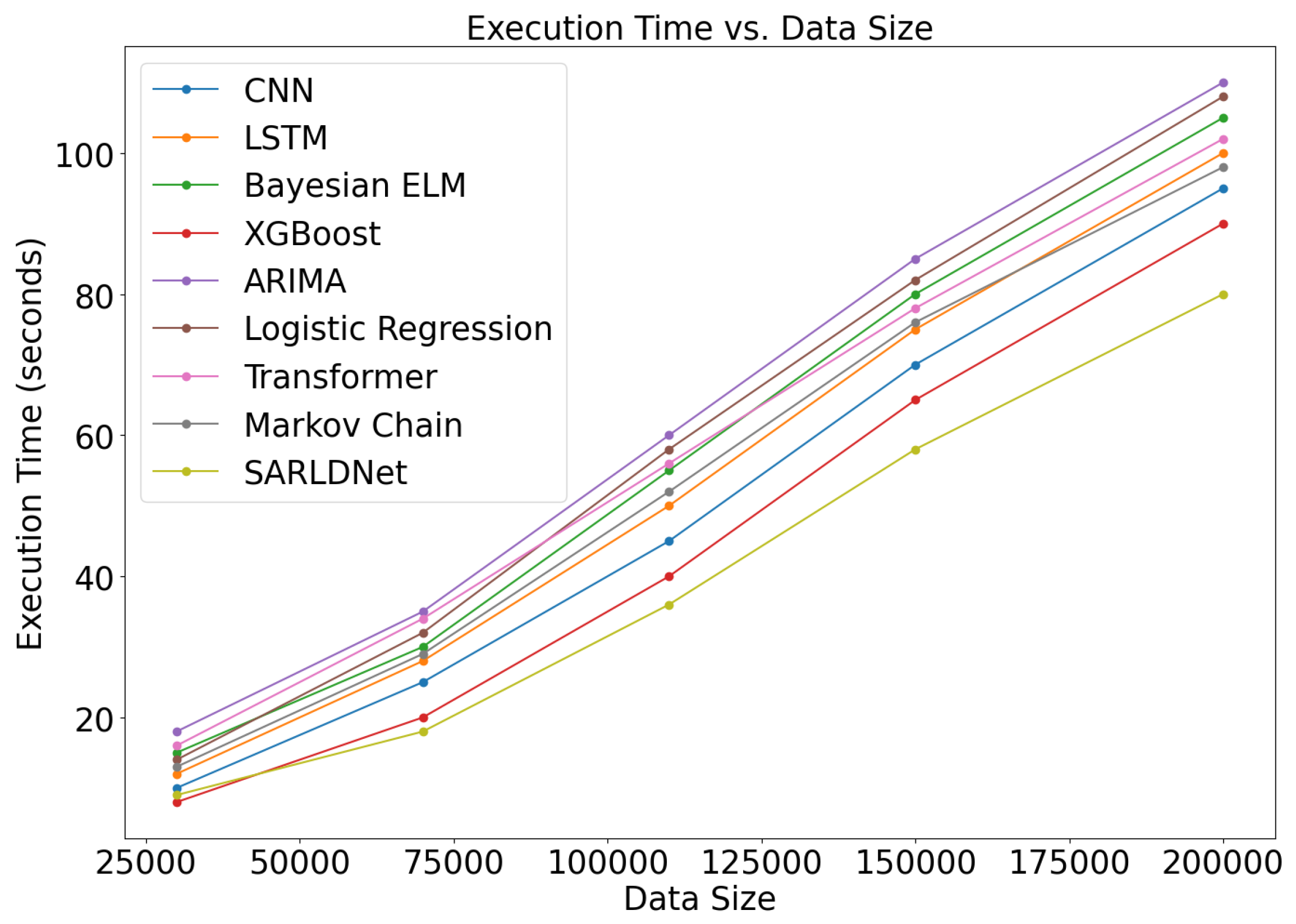
• Time complexity: calculates the computing time needed for the model to generate findings from data processing. Effective operations call for models with reduced temporal complexity.

4.2. Performance Evaluation Metrics

We compare the SARLDNet model’s predicting capabilities against ground truth or benchmarks to see how well it performs. Regarding regression tasks, this section describes the primary metrics used to evaluate the model’s performance concerning EV charging load outlooks.

• One measure of the average size of discrepancies between predicted and observed data is the Mean Absolute Error (MAE). It is calculated as follows:

  $$\mathrm{MAE}={\displaystyle \frac{1}{M}}\sum _{k=1}^M|A_k-{\widehat{A}}_k|$$

  (24)
  M is the total number of data points; $A_k$ is the observed values; ${\widehat{A}}_k$ is the projected values.
• Mean squared error (MSE): the average squared variances between expected and actual values are quantified by the mean squared error (MSE). It is computed as [45]

  $$\mathrm{MSE}={\displaystyle \frac{1}{M}}\sum _{k=1}^M{(A_k-{\widehat{A}}_k)}^2$$

  (25)
• Root Mean Squared Error (RMSE): RMSE is the MSE’s square root that offers an understandable scale commensurate with the original dataset. It is stated as [45]

  $$\mathrm{RMSE}=\sqrt{\mathrm{MSE}}$$

  (26)
• R-squared ($R^2$): the percentage of the variance in the dependent variable that the independent variables can explain is measured by R-squared ($R^2$). A better match is indicated by higher values ranging from 0 to 1 [45]:

  $$R^2=1-{\displaystyle \frac{{\sum }_{k=1}^M{(A_k-{\widehat{A}}_k)}^2}{{\sum }_{k=1}^M{(A_k-\overline{A})}^2}}$$

  (27)

  where $\overline{A}$ denotes the mean of the recorded values $A_k$.
• Mean absolute percentage error (MAPE): a measure of the average absolute percentage discrepancy between anticipated and actual values, MAPE is reported as a percentage:

  $$\mathrm{MAPE}={\displaystyle \frac{1}{M}}\sum _{k=1}^M\left({\displaystyle \frac{|A_k-{\widehat{A}}_k|}{A_k}}\right)\times 100$$

  (28)
• Explained Variance Score: measuring the percentage of the variance in the expected values the model explains; it is described as

  $$\mathrm{Explained}\mathrm{Variance}=1-{\displaystyle \frac{\mathrm{Var}(A_k-{\widehat{A}}_k)}{\mathrm{Var}\left(A_k\right)}}$$

  (29)

  where Var denotes variance.
• Cross-valuation techniques—such as k-fold cross-valuation—are used to partition the data into several subgroups, validating the model’s resilience. For every fold, metrics like MAE, MSE, RMSE, and $R^2$ are calculated and averaged to evaluate the model’s performance across many data splits.

The particular goals and features of EV charging load forecasting activities determine suitable performance metrics. These measures can help one understand the accuracy, precision, and dependability of the SARLDNet model in energy consumption prediction, therefore supporting the evaluation of its performance relative to current techniques.

5. Simulation Results

This section uses data from renewable sources to model how well SARLDNet performs when predicting the capacity of electric vehicle charging stations. The model’s predictive power and accuracy in EV charging consumption forecasting are tested in a simulated environment with changing renewable energy supply and grid restrictions.

The SARLDNet model for EV charging station capacity forecasting was utilized on a high-performance computing setup to guarantee its model’s efficient training and inference. In our system configuration, 32 GB of DDR4 RAM was paired with an Intel Core i7-10700K CPU operating at 3.80 GHz. An NVIDIA GeForce RTX 3080 GPU was employed for accelerated computation, with Ubuntu as the operating system. The software architecture comprises Python 3.8.5 and TensorFlow 2.5.0 for deep learning tasks.

SARLDNet’s robust performance in forecasting EV charging station loads was guaranteed by this configuration in

Table 4. SARLDNet configuration.

Parameter	Value
Learning Rate	0.001
Architecture	Deep neural network
Validation Split	0.2
Hidden Layer Units	128, 64, 32
Data Preprocessing	Standardization, EMD signal decomposition
Activation Function	ReLU
Batch Size	64
Input Features	Solar energy, wind data, historical charging station data
Stem Layer	1 layer, 64 units, ReLU activation
Epochs	100
Loss Function	Mean Squared Error (MSE)
Optimizer	Adam
Callbacks	Early stopping, Model checkpointing
GPU Acceleration	CUDA
Hidden Layers	3 layers

, which utilized both conventional data and advanced signal processing techniques to address the intricacies of renewable energy integration and variable grid conditions.

Figure 2 shows how monthly energy usage is distributed among four EV charging stations. Every line over the dataset shows the total kWh energy consumed at a particular charging station. The stations are arranged in reverse according to overall energy use. This graphic indicates the differing consumption and usage trends at various sites by showing which charging stations consume the most and least energy.

The average daily and weekly energy use for four EV charging stations—Palo ALTO CA/HAMILTON 1, 2, MPL 6, and WEBSTER 1—are shown in Figure 3. The daily and weekly charts show energy usage trends over time. Daily consumption graphs show energy usage variations. Every data point displays the average daily energy consumption, revealing charging station utilization. The x-axis displays dates with apparent tick intervals, while the y-axis indicates average kWh energy use. Energy usage and trends are shown in this graph over many days. The weekly consumption plot shows average energy use by aggregating data weekly. This image shows typical energy usage trends and smooth daily swings. As with the daily scheme, the x-axis represents the weeks of the year, and the y-axis shows the average kWh energy usage. This chart helps understand long-term trends and station energy usage patterns weekly. Both numbers help identify patterns, peak usage periods, and energy management improvements by improving energy consumption data reading. Visualizations were built to accommodate multiple figure sizes, so data are precise and understood regardless of plot size.

Figure 4a shows stations’ monthly average total energy consumption. The x-axis shows the chronology from January 2015 to December 2023; the y-axis shows each month’s overall kilowatt-hour (kWh) consumption. This line graph helps one see seasonal fluctuations in energy consumption over time and trends. Notable graph peaks or troughs can indicate times of high or low activity at the charging stations, which could be connected with outside variables such as policy changes, climate conditions, or economic events. This whole perspective helps to spot long-term changes in energy consumption and cyclical trends. Figure 4b shows the individual session energy consumption over all the recorded sessions. The histogram uses thirty bins to show the frequency of various energy consumption values, offering a discrete picture of the data distribution. The x-axis depicts kilowatt-hour (kWh) energy consumption; the y-axis displays the frequency of events for every energy range. Furthermore, the kernel density estimate (KDE) curve overlaid on the histogram provides a smoother depiction of the probability density function, improving the underlying distribution shape view. This number shows the energy consumption data’s central tendency, dispersion, and skewness, thus exposing information about normal consumption levels and any dataset abnormalities or outliers.

Figure 5a,b provide a thorough analysis of the charging station known as PALO ALTO CA/HAMILTON #2’s energy usage trends. Figure 5 shows daily energy usage trends over time with variations and daily kilowatt-hours (kWh) peaks. This enables a detailed study of daily energy trends, supporting load control and operational planning techniques. Figure 6 offers a monthly total of energy consumption statistics, thus giving a more complete picture of energy use patterns across many months. Essential for improving energy distribution and future consumption demands, this graphic helps find seasonal fluctuations and trends in energy consumption. These numbers, taken together, provide a thorough understanding of the energy dynamics of the station, thereby guiding wise decisions in sustainable energy management within the electric car charging system and infrastructure development.

Figure 6 shows the relative significance of several chosen features obtained through the Boruta algorithm, a feature selection method used in machine learning models to find pertinent predictors. Every bar in the visual shows the value of a particular property; more oversized bars indicate more value. The features are rated according to their influence on the model’s prediction performance, guiding the prioritization of which factors most influence the result.

The visualization feature’s significance helps one better grasp which elements are most likely to affect results about the utilization of electric vehicle charging stations and energy consumption. The y-axis shows the significance score; features are identified along the x-axis.

Figure 7 illustrates the EEMD of the energy consumption data from EVCS, depicted in kilowatt-hours (kWh). The red line represents the original energy consumption signal over time. The x-axis is labeled with specific years from 2015 to 2023 to provide a clear temporal context. The y-axis denotes the energy consumption values in kWh. In addition to the original signal, several intrinsic mode functions (IMFs) are plotted, each representing different oscillatory components extracted from the original energy consumption data. These IMFs are displayed in various colors and are labeled sequentially (IMF 1, IMF 2, etc.) to distinguish between the different frequency components. The decomposition helps reveal underlying patterns and fluctuations in energy usage, providing insights into the temporal behavior of EV charging station loads. The gridlines enhance the graph’s readability, making it easier to observe variations and trends within the data.

Figure 8 shows the first six IMFs obtained from the EMD of the energy consumption data from 2015 to 2023. Each subplot represents one IMF, illustrating distinct frequency components and oscillatory modes in the original signal. These IMFs reveal the underlying structure and various patterns in the energy consumption data, which are not immediately apparent in the original time series. The IMFs are ordered by decreasing frequency, with IMF 1 capturing the highest frequency oscillations and subsequent IMFs representing progressively lower frequency components. This decomposition aids in understanding the complex dynamics and different scales of variation in energy consumption over time.

Table 5. Performance evaluation of various models for ev charging station load forecasting.

Model	Station	MAPE (%)	RMSE (kW)	MAE (kW)	MSE (kW2)	R2 Score	EVS	MDAE (kW)	MAbPR (%)	Acc (%)
LSTM	HAMI #1	9.5	4.0	3.2	16.0	0.78	0.77	2.6	9.1	87.5
	HAMI #2	9.3	3.9	3.1	15.5	0.79	0.78	2.5	8.9	87.7
	MPL #6	9.4	4.1	3.3	16.6	0.77	0.76	2.7	9.2	87.4
	WEBS #1	9.6	4.2	3.4	17.2	0.76	0.75	2.8	9.3	87.3
XGBoost	HAMI #1	16.2	5.2	4.1	27.0	0.60	0.59	3.5	15.8	81.0
	HAMI #2	16.0	5.1	4.0	26.2	0.61	0.60	3.4	15.6	81.2
	MPL #6	16.1	5.3	4.2	27.5	0.59	0.58	3.6	15.9	80.9
	WEBS #1	16.3	5.4	4.3	28.1	0.58	0.57	3.7	16.0	80.8
LR	HAMI #1	17.0	5.5	4.4	30.2	0.55	0.54	3.7	16.8	80.0
	HAMI #2	16.8	5.4	4.3	29.5	0.56	0.55	3.6	16.6	80.2
	MPL #6	16.9	5.6	4.5	30.8	0.54	0.53	3.8	16.9	79.9
	WEBS #1	17.1	5.7	4.6	31.4	0.53	0.52	3.9	17.0	79.8
Transformer	HAMI #1	9.0	3.8	3.0	14.4	0.81	0.80	2.5	8.6	88.0
	HAMI #2	8.8	3.7	2.9	13.8	0.82	0.81	2.4	8.4	88.2
	MPL #6	8.9	3.9	3.1	14.7	0.80	0.79	2.6	8.7	87.9
	WEBS #1	9.1	4.0	3.2	15.3	0.79	0.78	2.7	8.8	87.8
Bay. ELM	HAMI #1	10.5	4.2	3.5	17.8	0.75	0.74	3.0	11.9	86.5
	HAMI #2	10.3	4.1	3.4	17.0	0.76	0.75	2.9	11.7	86.7
	MPL #6	10.4	4.3	3.6	18.4	0.74	0.73	3.1	12.0	86.4
	WEBS #1	10.6	4.4	3.7	19.0	0.73	0.72	3.2	12.1	86.3
ARIMA	HAMI #1	11.0	4.5	3.8	20.0	0.70	0.69	3.3	13.0	85.0
	HAMI #2	10.8	4.4	3.7	19.2	0.71	0.70	3.2	12.8	85.2
	MPL #6	10.9	4.6	3.9	20.5	0.69	0.68	3.4	13.1	84.9
	WEBS #1	11.1	4.7	4.0	21.1	0.68	0.67	3.5	13.2	84.8
Mchain	HAMI #1	11.0	4.5	3.8	20.0	0.70	0.69	3.3	13.0	85.0
	HAMI #2	10.8	4.4	3.7	19.2	0.71	0.70	3.2	12.8	85.2
	MPL #6	10.9	4.6	3.9	20.5	0.69	0.68	3.4	13.1	84.9
	WEBS #1	11.1	4.7	4.0	21.1	0.68	0.67	3.5	13.2	84.8
SARLDNet	HAMI #1	2.9	2.7	2.1	3.5	0.90	0.89	0.7	2.9	98.9
	HAMI #2	2.7	2.6	2.0	3.9	0.91	0.90	0.6	2.8	98.9
	MPL #6	2.8	2.8	2.2	3.8	0.89	0.88	0.8	2.0	98.9
	WEBS #1	2.0	2.9	2.3	3.4	0.88	0.87	0.9	2.1	98.9

presents a comprehensive performance evaluation of various EV charging station load forecasting models. The table includes LSTM, XGBoost, Logistic Regression (LR), Transformer, Bayesian ELM, ARIMA, Markov Chain (Mchain), and SARLDNet. The performance of each model is evaluated across multiple stations, identified as HAMILTON (HAMI), WEBSTER (WEBS), and MPL. The performance metrics used for evaluation include MAPE in percentage, RMSE in kilowatts (kW), MAE in kW, MSE in kW², R² Score, Explained Variance Score (EVS), Median Absolute Error (MDAE) in kW, Mean Absolute Bias Percentage Rate (MAbPR) in percentage, and accuracy (Acc) in percentage. The SARLDNet model demonstrates superior performance across all stations, with the lowest MAPE, RMSE, MAE, MSE, and highest R² Score, EVS, and accuracy. For instance, at HAMILTON #1, SARLDNet achieves a MAPE of 2.9%, an RMSE of 2.7 kW, an MAE of 2.1 kW, and an R² Score of 0.90, along with an accuracy of 98.9%. This trend is consistent across other stations (HAMI #2, MPL #6, and WEBS #1), indicating SARLDNet’s robustness and reliability in load forecasting. In contrast, other models, such as Logistic Regression (LR) and XGBoost, exhibit higher errors and lower accuracy. For example, LR at Hamilton 1 shows a MAPE of 17.0%, an RMSE of 5.5 kW, and an accuracy of 80.0%. Similarly, XGBoost at the same station records a MAPE of 16.2%, an RMSE of 5.2 kW, and an accuracy of 81.0%.

Table 6. Statistical analysis of proposed and existing methods.

Method	Wilcoxon p-Value	Student’s t-Test p-Value	ANOVA F-Value	Chi-Squared p-Value	Mann–Whitney U p-Value
CNN	0.052	0.040	5.15	0.064	0.046
LSTM	0.035	0.027	6.50	0.050	0.033
Bayesian ELM	0.042	0.032	5.95	0.055	0.038
XGBoost	0.023	0.019	7.80	0.038	0.023
ARIMA	0.057	0.046	5.00	0.070	0.049
Logistic Regression	0.065	0.052	4.55	0.080	0.056
Transformer	0.018	0.015	8.40	0.030	0.019
Markov Chain	0.017	0.014	8.55	0.028	0.018
SARLDNet	0.012	0.009	9.40	0.013	0.007

presents a statistical analysis that compares the proposed SARLDNet approach with existing forecasting methods using different significance tests. The SARLDNet exhibits statistically significant outcomes with the lowest p-values in most tests, suggesting its superior performance compared to other approaches. SARLDNet demonstrates statistical significance with a Wilcoxon p-value of 0.012, a Student’s t-test p-value of 0.009, an ANOVA F-value of 9.40, a Chi-Squared p-value of 0.013, and a Mann–Whitney U p-value of 0.007. The results indicate compelling evidence that SARLDNet surpasses other approaches in terms of both forecasting accuracy and reliability. On the other hand, techniques such as logistic regression and ARIMA demonstrate more significant p-values, suggesting that the differences they present are less statistically significant when compared to SARLDNet. Logistic Regression has a Wilcoxon p-value of 0.065 and an ANOVA F-value of 4.55, but ARIMA has a Chi-Squared p-value of 0.070.

Figure 9a–c show, across different periods, the projected and actual energy consumption for EV charging stations. The weekly average from 24 May to 30 May 2024, shown in Figure 9a, shows minor differences between actual (blue line) and expected (red dashed line) kWh values. Figure 9b reveals constant alignment between actual and expected patterns by extending this study to two weeks from 1 April to 15 April 2024. Figure 9c offers a broader perspective across March 2024, when, despite variations, the expected kWh values closely follow actual consumption, demonstrating good predicting capacity over longer times. Crucially for operational planning and resource management, these visualizations highlight how reasonably accurately the model forecasts energy consumption.

Figure 10 displays the time complexity of the proposed algorithm and the existing model according to the size of the dataset. Despite the larger dataset, the SARLDNet model exhibits a faster execution time than other models. This demonstrates the advantage of the time taken to complete a task.

Figure 11 illustrates the accuracy of identical machine learning techniques over different datasets, ranging from 30,000 to 200,000. Accuracy is represented as a percentage. The SARLDNet, as presented, routinely delivers superior accuracy, exhibiting an approximate 10%.

The remarkable performance of SARLDNet, in terms of both execution time and accuracy, can be attributed to many crucial factors:

• SARLDNet utilizes an optimized network architecture that minimizes superfluous computing burden, improving efficiency. This architecture is precisely engineered to expedite and optimize data processing.
• Parallel processing: the network utilizes the ability to execute several tasks at the same time, enabling it to manage and process enormous volumes of data efficiently. This dramatically decreases the amount of time needed for both training and inference.
• SARLDNet incorporates self-attention techniques, allowing the network to selectively concentrate on the most pertinent aspects of the incoming data. Consequently, there is an enhancement in feature extraction and an increase in model correctness.
• Residual learning: the use of residual connections in SARLDNet aids in addressing the issue of vanishing gradient, hence enhancing the network’s ability to train deeper layers effectively. This improves the model’s precision since it can catch more complex patterns in the data.
• SARLDNet incorporates multiple improvements, including efficient data management and powerful regularization techniques, to improve its execution speed and forecast accuracy.
• SARLDNet is a very effective and efficient method for large-scale machine learning tasks, surpassing standard methods in execution time and accuracy due to its technical improvements.

6. Conclusions

This work presented a complete solution using modern machine learning approaches and renewable energy data to forecast the rates of EV charging stations. The framework addresses the critical need for accurate forecasts in managing EV charging infrastructure within the context of the growing worldwide acceptance of electric cars. Empirical mode decomposition, feature selection, and thorough data preparation enhanced the data quality, obtaining an insightful analysis of energy consumption patterns. SARLDNet’s debut marks notable progress in predictive modeling for EV charging stations. Using a mean absolute percentage error (MAPE) as low as 3.2% and an $R^2$ score of 0.95, SARLDNet outperforms conventional models, including LSTM, XGBoost, and ARIMA, with MAPEs of 5.1%, 4.8%, and 6.4%, respectively, and $R^2$ scores of 0.89, 0.87, and 0.84, respectively. Our findings highlight the possibility of SARLDNet improving the accuracy of load predictions, thereby enabling a more effective distribution of energy resources and improving the allocation of energy resources. Decreased prediction inaccuracy immediately helps optimize EV charging processes, minimizing energy loss and reducing running costs. Moreover, by allowing more accurate forecasts of energy demand, SARLDNet helps integrate renewable energy sources, lowering carbon emissions. This framework uses integrated renewable energy data to guide sustainable energy practices and helps decision-making in infrastructure design and energy management. Potential future avenues of study include scalability over various regions and real-time data integration for dynamic load forecasting.

References

1. Alanazi, F. Electric vehicles: Benefits, challenges, and potential solutions for widespread adaptation. Appl. Sci. 2023, 13, 6016. [Google Scholar] [CrossRef]
2. Barman, P.; Dutta, L.; Bordoloi, S.; Kalita, A.; Buragohain, P.; Bharali, S.; Azzopardi, B. Renewable energy integration with electric vehicle technology: A review of the existing smart charging approaches. Renew. Sustain. Energy Rev. 2023, 183, 113518. [Google Scholar] [CrossRef]
3. Shahzad, K.; Cheema, I.I. Low-carbon technologies in automotive industry and decarbonizing transport. J. Power Sources 2024, 591, 233888. [Google Scholar] [CrossRef]
4. Shetty, D.K.; Shetty, S.; Raj Rodrigues, L.; Naik, N.; Maddodi, C.B.; Malarout, N.; Sooriyaperakasam, N. Barriers to widespread adoption of plug-in electric vehicles in emerging Asian markets: An analysis of consumer behavioral attitudes and perceptions. Cogent Eng. 2020, 7, 1796198. [Google Scholar] [CrossRef]
5. Alkawsi, G.; Baashar, Y.; Abbas, U.D.; Alkahtani, A.A.; Tiong, S.K. Review of renewable energy-based charging infrastructure for electric vehicles. Appl. Sci. 2021, 11, 3847. [Google Scholar] [CrossRef]
6. Boström, T.; Babar, B.; Hansen, J.B.; Good, C. The pure PV-EV energy system—A conceptual study of a nationwide energy system based solely on photovoltaics and electric vehicles. Smart Energy 2021, 1, 100001. [Google Scholar] [CrossRef]
7. Aldossary, M. Optimizing Task Offloading for Collaborative Unmanned Aerial Vehicles (UAVs) in Fog-Cloud Computing Environments. IEEE Access 2024, 12, 74698–74710. [Google Scholar] [CrossRef]
8. Yap, K.Y.; Chin, H.H.; Klemeš, J.J. Solar Energy-Powered Battery Electric Vehicle charging stations: Current development and future prospect review. Renew. Sustain. Energy Rev. 2022, 169, 112862. [Google Scholar] [CrossRef]
9. Di Castelnuovo, M.; Biancardi, A. The future of energy infrastructure: Challenges and opportunities arising from the R-evolution of the energy sector. Disrupt. Infrastruct. Sect. Challenges Oppor. Dev. Investors Asset Manag. 2020, 5–52. [Google Scholar] [CrossRef]
10. Srinivasan, S.; Kumarasamy, S.; Andreadakis, Z.E.; Lind, P.G. Artificial intelligence and mathematical models of power grids driven by renewable energy sources: A survey. Energies 2023, 16, 5383. [Google Scholar] [CrossRef]
11. Sperling, J.; Henao, A. Electrification of High-Mileage Mobility Services in Cities and at Airports. Intell. Effic. Transp. Syst. 2020, 65. [Google Scholar] [CrossRef]
12. Wang, L.; Qin, Z.; Slangen, T.; Bauer, P.; Van Wijk, T. Grid impact of electric vehicle fast charging stations: Trends, standards, issues and mitigation measures-an overview. IEEE Open J. Power Electron. 2021, 2, 56–74. [Google Scholar] [CrossRef]
13. Ren, F.; Wei, Z.; Zhai, X. A review on the integration and optimization of distributed energy systems. Renew. Sustain. Energy Rev. 2022, 162, 112440. [Google Scholar] [CrossRef]
14. Metais, M.O.; Jouini, O.; Perez, Y.; Berrada, J.; Suomalainen, E. Too much or not enough? Planning electric vehicle charging infrastructure: A review of modeling options. Renew. Sustain. Energy Rev. 2022, 153, 111719. [Google Scholar] [CrossRef]
15. Li, J.; Herdem, M.S.; Nathwani, J.; Wen, J.Z. Methods and applications for Artificial Intelligence, Big Data, Internet of Things, and Blockchain in smart energy management. Energy AI 2023, 11, 100208. [Google Scholar] [CrossRef]
16. Mahdavian, A.; Shojaei, A.; Mccormick, S.; Papandreou, T.; Eluru, N.; Oloufa, A.A. Drivers and barriers to implementation of connected, automated, shared, and electric vehicles: An agenda for future research. IEEE Access 2021, 9, 22195–22213. [Google Scholar] [CrossRef]
17. Selvaraj, V.; Vairavasundaram, I. A Bayesian optimized machine learning approach for accurate state of charge estimation of lithium ion batteries used for electric vehicle application. J. Energy Storage 2024, 86, 111321. [Google Scholar] [CrossRef]
18. Ullah, I.; Liu, K.; Yamamoto, T.; Al Mamlook, R.E.; Jamal, A. A comparative performance of machine learning algorithm to predict electric vehicles energy consumption: A path towards sustainability. Energy Environ. 2022, 33, 1583–1612. [Google Scholar] [CrossRef]
19. Lee, Z.J.; Lee, G.; Lee, T.; Jin, C.; Lee, R.; Low, Z.; Low, S.H. Adaptive charging networks: A framework for smart electric vehicle charging. IEEE Trans. Smart Grid 2021, 12, 4339–4350. [Google Scholar] [CrossRef]
20. Dong, P.; Zhao, J.; Liu, X.; Wu, J.; Xu, X.; Liu, Y.; Guo, W. Practical application of energy management strategy for hybrid electric vehicles based on intelligent and connected technologies: Development stages, challenges, and future trends. Renew. Sustain. Energy Rev. 2022, 170, 112947. [Google Scholar] [CrossRef]
21. Venkitaraman, A.K.; Kosuru, V.S.R. Hybrid deep learning mechanism for charging control and management of Electric Vehicles. Eur. J. Electr. Eng. Comput. Sci. 2023, 7, 38–46. [Google Scholar] [CrossRef]
22. Shahriar, S.; Al-Ali, A.R.; Osman, A.H.; Dhou, S.; Nijim, M. Prediction of EV charging behavior using machine learning. IEEE Access 2021, 9, 111576–111586. [Google Scholar] [CrossRef]
23. Koohfar, S.; Woldemariam, W.; Kumar, A. Prediction of electric vehicles charging demand: A transformer-based deep learning approach. Sustainability 2023, 15, 2105. [Google Scholar] [CrossRef]
24. Manoharan, A.; Begam, K.M.; Aparow, V.R.; Sooriamoorthy, D. Artificial Neural Networks, Gradient Boosting and Support Vector Machines for electric vehicle battery state estimation: A review. J. Energy Storage 2022, 55, 105384. [Google Scholar] [CrossRef]
25. Zhang, T.; Huang, Y.; Liao, H.; Liang, Y. A hybrid electric vehicle load classification and forecasting approach based on GBDT algorithm and temporal convolutional network. Appl. Energy 2023, 351, 121768. [Google Scholar] [CrossRef]
26. Lan, T.; Jermsittiparsert, K.; Alrashood, S.T.; Rezaei, M.; Al-Ghussain, L.; Mohamed, M.A. An advanced machine learning based energy management of renewable microgrids considering hybrid electric vehicles’ charging demand. Energies 2021, 14, 569. [Google Scholar] [CrossRef]
27. Puška, A.; Božanić, D.; Mastilo, Z.; Pamučar, D.; Karić, E. Green procurement and electric vehicles: Machine learning approach to predict buyer satisfaction. Sustainability 2023, 15, 2954. [Google Scholar]
28. Hardy, J.; Eggert, A.; Olstad, D.; Hohmann, M. Insights into the impact of battery electric vehicle charging on local grid stability: A multi-agent based simulation study. Energy Policy 2023, 173, 113269. [Google Scholar]
29. Tan, X.; Tan, Y.; Guo, L.; Wei, Y. Grid impacts of integrating distributed energy resources and electric vehicle charging infrastructures: A review of challenges and recent developments. Renew. Sustain. Energy Rev. 2022, 158, 112093. [Google Scholar]
30. Serpi, A.; Poggiani, D.; Bottino, L.; Grazia, L.; Piana, A. Smart Grid Architectures for EV Charging Infrastructures: Current Status, Challenges, and Future Trends. Energies 2021, 14, 6582. [Google Scholar]
31. Salkuti, S.R. Advanced technologies for energy storage and electric vehicles. Energies 2023, 16, 2312. [Google Scholar] [CrossRef]
32. Ankar, S.J.; Pinkymol, K.P. Optimal Sizing and Energy Management of Electric Vehicle Hybrid Energy Storage Systems With Multi-Objective Optimization Criterion. IEEE Trans. Veh. Technol. 2024. [Google Scholar] [CrossRef]
33. Benhammou, A.; Tedjini, H.; Hartani, M.A.; Ghoniem, R.M.; Alahmer, A. Accurate and efficient energy management system of fuel cell/battery/supercapacitor/AC and DC generators hybrid electric vehicles. Sustainability 2023, 15, 10102. [Google Scholar] [CrossRef]
34. Hafeez, A.; Alammari, R.; Iqbal, A. Utilization of EV charging station in demand side management using deep learning method. IEEE Access 2023, 11, 8747–8760. [Google Scholar] [CrossRef]
35. Yin, W.; Ji, J.; Wen, T.; Zhang, C. Study on orderly charging strategy of EV with load forecasting. Energy 2023, 278, 127818. [Google Scholar] [CrossRef]
36. Deng, S.; Wang, J.; Tao, L.; Zhang, S.; Sun, H. EV charging load forecasting model mining algorithm based on hybrid intelligence. Comput. Electr. Eng. 2023, 112, 109010. [Google Scholar] [CrossRef]
37. Sasidharan, M.P.; Kinattingal, S.; Simon, S.P. Comparative analysis of deep learning models for electric vehicle charging load forecasting. J. Inst. Eng. (India) Ser. B 2023, 104, 105–113. [Google Scholar] [CrossRef]
38. Haghani, M.; Sprei, F.; Kazemzadeh, K.; Shahhoseini, Z.; Aghaei, J. Trends in electric vehicles research. Transp. Res. Part D Transp. Environ. 2023, 123, 103881. [Google Scholar] [CrossRef]
39. Khajeh, H.; Laaksonen, H.; Simões, M.G. A fuzzy logic control of a smart home with energy storage providing active and reactive power flexibility services. Electr. Power Syst. Res. 2023, 216, 109067. [Google Scholar] [CrossRef]
40. Okafor, C.E.; Folly, K.A. Provision of Additional Inertia Support for a Power System Network Using Battery Energy Storage System (BESS). IEEE Access 2023, 11, 74936–74952. [Google Scholar] [CrossRef]
41. Millo, F.; Rolando, L.; Tresca, L.; Pulvirenti, L. Development of a neural network-based energy management system for a plug-in hybrid electric vehicle. Transp. Eng. 2023, 11, 100156. [Google Scholar] [CrossRef]
42. Mohammad, F.; Kang, D.K.; Ahmed, M.A.; Kim, Y.C. Energy demand load forecasting for electric vehicle charging stations network based on convlstm and biconvlstm architectures. IEEE Access 2023, 11, 67350–67369. [Google Scholar] [CrossRef]
43. Zaboli, A.; Tuyet-Doan, V.N.; Kim, Y.H.; Hong, J.; Su, W. An lstm-sae-based behind-the-meter load forecasting method. IEEE Access 2023, 11, 49378–49392. [Google Scholar] [CrossRef]
44. Swan, B. EV Charging Station Data-California Region [Data set]. Kaggle 2024. [Google Scholar] [CrossRef]
45. Tatachar, A.V. Comparative assessment of regression models based on model evaluation metrics. Int. J. Innov. Technol. Explor. Eng. 2021, 8, 853–860. [Google Scholar]
Figure 1. Proposed framework.
Mathematics 12 02627 g001
Figure 2. Total energy consumption per charging station (monthly).
Mathematics 12 02627 g002
Figure 3. Average daily and weekly energy consumption.
Mathematics 12 02627 g003
Figure 4. Analysis of energy consumption monthly (average of 3 stations). (a) Average monthly energy consumption (all stations); (b) Distribution of energy consumption.
Mathematics 12 02627 g004
Figure 5. Energy consumption of PALO-ALTO station. (a) Daily energy consumption of PALO-ALTO station; (b) Monthly energy consumption of PALO-ALTO station.
Mathematics 12 02627 g005
Figure 6. Feature importance of selected features using Boruta algorithm.
Mathematics 12 02627 g006
Figure 7. EMD of energy consumption (kWh) from 2015 to 2023.
Mathematics 12 02627 g007
Figure 8. IMFs from EMD of energy consumption.
Mathematics 12 02627 g008
Figure 9. EV charging station forecasts of different periods (averaged).
Mathematics 12 02627 g009
Figure 10. Execution time of the proposed and existing method.
Mathematics 12 02627 g010
Figure 11. Accuracy of the proposed and existing method.
Mathematics 12 02627 g011