H_∞ Differential Game of Nonlinear Half-Car Active Suspension via Off-Policy Reinforcement Learning

Abstract

This paper investigates a parameter-free H_∞ differential game approach for nonlinear active vehicle suspensions. The study accounts for the geometric nonlinearity of the half-car active suspension and the cubic nonlinearity of the damping elements. The nonlinear H_∞ control problem is reformulated as a zero-sum game between two players, leading to the establishment of the Hamilton–Jacobi–Isaacs (HJI) equation with a Nash equilibrium solution. To minimize reliance on model parameters during the solution process, an actor–critic framework employing neural networks is utilized to approximate the control policy and value function. An off-policy reinforcement learning method is implemented to iteratively solve the HJI equation. In this approach, the disturbance policy is derived directly from the value function, requiring only a limited amount of driving data to approximate the HJI equation’s solution. The primary innovation of this method lies in its capacity to effectively address system nonlinearities without the need for model parameters, making it particularly advantageous for practical engineering applications. Numerical simulations confirm the method’s effectiveness and applicable range. The off-policy reinforcement learning approach ensures the safety of the design process. For low-frequency road disturbances, the designed H_∞ control policy enhances both ride comfort and stability.

1. Introduction

The active suspension system is a critical component for intelligent vehicle operation, significantly impacting driving, steering, braking, and obstacle navigation [1]. With advancements in actuators and drive-by-wire technology, the application of active suspensions is becoming increasingly widespread. Particularly during the pilot phase of intelligent driving technology, active suspension control based on AI large models has emerged as a challenging and vital research area [2,3].

In recent years, researchers have proposed numerous actuator and controller design methods for active suspension systems, including air suspension, electromagnetic suspension, and a magneto-rheological damper [4,5,6]. Reference [7] investigated finite-time neural control of electromagnetic suspension, taking partial actuator failures into account. Reference [8] designed a static output feedback controller for active suspension, which reduces implementation costs. With the advancement of sensing technology, road preview-based active suspension control techniques have also been developed, such as wheelbase preview control [9,10] and comfort-oriented longitudinal velocity planning [11].

In the design of active suspension control, it is crucial to consider the system’s nonlinearity and fault tolerance. References [12,13] developed a nonlinear model predictive controller and a robust fault-tolerant controller with saturation for a quarter-car active suspension, achieving favorable practical results. Additionally, various robust control methods have been extensively researched, including finite-time H_∞ control [14], fuzzy sampled H_∞ control [15], and finite-frequency H_∞ control [16], all of which address system robustness. Reference [17] explored model predictive control for active suspension, achieving optimal control performance while satisfying constraints. However, most methods assume known model parameters or only consider vertical dynamics, with limited focus on nonlinear coupling models in complex and variable environments. Some researchers have investigated model-free control methods, such as neuro-fuzzy H₂/H_∞ control [18], adaptive optimal control based on neural networks [19], and approximation-free preset-time control [20]. Given that parameter calibration is time-consuming and parameters often vary in complex and dynamic environments, model-free control methods are more practical for real-world applications.

As a technical approach within AI large models, data-driven reinforcement learning (RL) methods have garnered considerable attention. References [21,22,23] proposed data-driven optimal control methods for active suspensions, utilizing driving data to train and optimize control policies. Data-driven RL algorithms are highly effective for nonlinear H_∞ differential games, nonlinear optimal control, static output-feedback, and event-triggered control [24,25,26]. While some researchers have applied data-driven RL methods to active suspensions, most have only considered vertical dynamics, neglecting the nonlinear coupling characteristics of front and rear wheels and pitch stability. In previous studies on H_∞ control [21,23,27,28], the system is typically assumed to be linear, and only simplified quarter-car active suspension models are considered, which deviates from real-world scenarios. Additionally, most methods require system model parameters, which inevitably increase control costs and complexity. This is the primary motivation for our research. In summary, research on nonlinear H_∞ differential games for active suspensions remains insufficient. This paper establishes a more realistic half-car active suspension model and transforms the nonlinear H_∞ control problem into a differential game between two players. An off-policy RL algorithm, which does not require model parameters, is designed to approximate the solution to the Hamilton–Jacobi–Isaacs (HJI) equation by collecting a portion of vehicle vibration data. Finally, the effectiveness of control optimization and implementation is verified through hardware-in-the-loop simulation, and the effective vibration reduction range of the control policy is analyzed in detail. The main contributions of this paper are as follows:

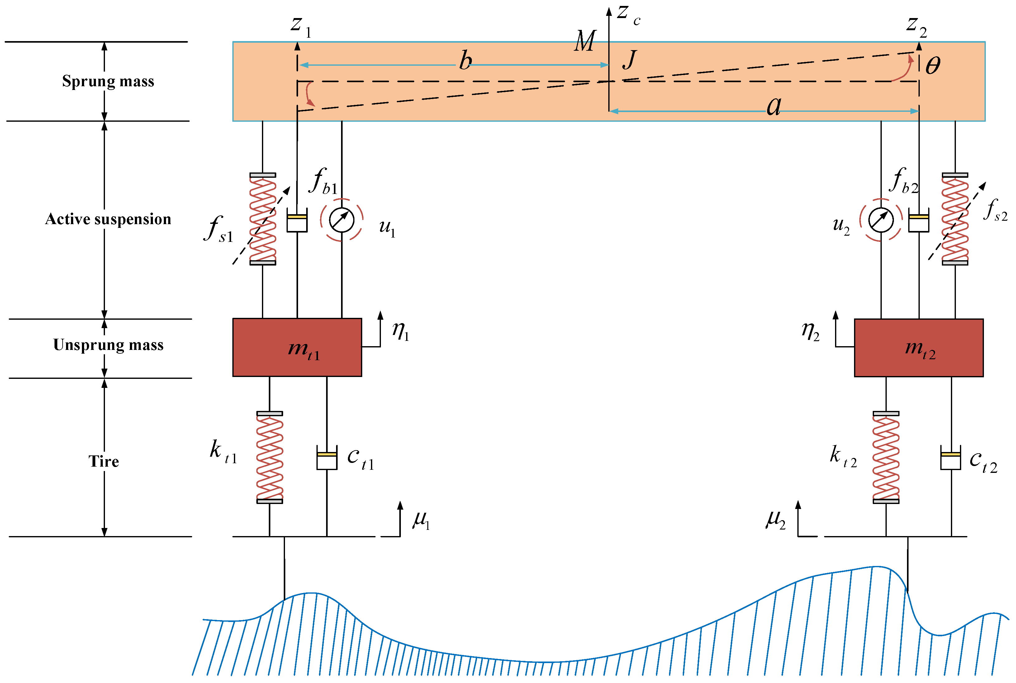
• To enhance the vibration control performance of active suspension systems, a more realistic half-car suspension dynamics model is established, and a nonlinear H_∞ differential game method is proposed;
• A neural network-based approach is utilized to derive an off-policy RL algorithm for solving the HJI equation, providing an optimal solution without requiring any model parameters;
• A hardware-in-the-loop simulation platform is developed, validating the effectiveness and feasibility of the proposed method through numerical simulations.

The remainder of the paper is structured as follows. Section 2 introduces the nonlinear half-car active suspension control model. Section 3 describes the methodology in detail. Section 4 presents the numerical simulation results. Section 5 concludes with a summary of the findings.

2. Mathematical Model

To represent the nonlinear coupling relationship between the front and rear suspensions, a widely used half-car active suspension model is established, as shown in Figure 1, with the symbols defined in

Table 1. Symbol definitions.

Symbol	Meaning
$M$	Sprung mass
$J$	Pitch moment of inertia
$m_{t1}$, $m_{t2}$	Unsprung mass
$a$	Distance from front axle to center of mass
$b$	Distance from rear axle to center of mass
$k_{t1}$, $k_{t2}$	Tire stiffness
$k_{s1}$, $k_{s2}$	Suspension spring linear stiffness
$k_{sn1}$, $k_{sn2}$, $k_{sn3}$, $k_{sn4}$	Suspension spring nonlinear stiffness
$b_{s1}$, $b_{s2}$	Suspension hydraulic linear damping
$b_{sn1}$, $b_{sn2}$	Suspension hydraulic nonlinear damping
$u_1$, $u_2$	Active control force
$z_c$	Vertical displacement of the center of mass
$\theta$	Pitch angle
${\eta }_1$, ${\eta }_2$	Vertical displacement of unsprung mass
${\mu }_1$, ${\mu }_2$	Road disturbance

. According to the second kind of Lagrange’s equations, the dynamic equations for the half-car active suspension are as follows [9,10,29,30]:

$$\begin{array}{c}M{\ddot{z}}_c=f_1+f_2\\ J\ddot{\theta }=a{f}_1-b{f}_2\\ m_{t1}{\ddot{\eta }}_1=-k_{t1}\left({\eta }_1-{\mu }_1\right)-f_1\\ m_{t2}{\ddot{\eta }}_2=-k_{t2}\left({\eta }_2-{\mu }_2\right)-f_2\end{array}$$

(1)

where

$$\begin{array}{l}{f}_1=f_{s1}+f_{d1}+u_1\\ f_2=f_{s2}+f_{d2}+u_2\\ f_{s1}=k_{s1}\left({\eta }_1-z_1\right)+k_{sn1}{\left({\eta }_1-z_1\right)}^2+k_{sn2}{\left({\eta }_1-z_1\right)}^3\\ f_{d1}=b_{s1}\left({\dot{\eta }}_2-{\dot{z}}_2\right)+b_{sn1}{\left({\dot{\eta }}_2-{\dot{z}}_2\right)}^2\\ f_{s2}=k_{s2}\left({\eta }_2-z_2\right)+k_{sn3}{\left({\eta }_1-z_1\right)}^2+k_{sn4}{\left({\eta }_1-z_1\right)}^3\\ f_{d2}=b_{s2}\left({\dot{\eta }}_2-{\dot{z}}_2\right)+b_{sn2}{\left({\dot{\eta }}_2-{\dot{z}}_2\right)}^2\end{array}$$

In Equation (1), the quadratic and cubic nonlinearities of the spring and damper are considered, along with the nonlinear coupling of the front and rear suspensions. For larger road excitations, these nonlinear characteristics should not be ignored.

Define

$$\begin{array}{l}{z}_1=z_c+a\sin \theta \\ z_2=z_c-b\sin \theta \end{array}$$

(2)

Choose the state variables of the system as

$$x={\left[\begin{array}{cccccccc}{x}_1& x_2& x_3& x_4& x_5& x_6& x_7& x_8\end{array}\right]}^T$$

(3)

where

$$\begin{array}{c}{x}_1=z_c+a\sin \theta -{\eta }_1, x_2=z_c-b\sin \theta -{\eta }_2, x_3={\eta }_1-{\mu }_1, x_4={\eta }_2-{\mu }_2,\\ x_5={\dot{z}}_c+a\cos \theta \cdot \dot{\theta }, x_6={\dot{z}}_c-b\cos \theta \cdot \dot{\theta }, x_7={\dot{\eta }}_1, x_8={\dot{\eta }}_2\end{array}$$

Define

$$a_1={\displaystyle \frac{1}{M}}+{\displaystyle \frac{a^2\cos \theta }{J}}, a_2={\displaystyle \frac{1}{M}}-{\displaystyle \frac{ab\cos \theta }{J}}, a_3={\displaystyle \frac{1}{M}}+{\displaystyle \frac{b^2\cos \theta }{J}}$$

(4)

combining Equations (1) to (4), the nonlinear state-space equations of the half-car active suspension are obtained:

$$\begin{array}{c}\dot{x}\left(t\right)=A\left(x\right)+B\left(x\right)u+C\omega \\ y\left(t\right)=x\left(t\right)\end{array}$$

(5)

where

$$\begin{array}{c}A\left(x\right)=\left[\begin{array}{c}{x}_5-x_7\\ x_6-x_8\\ x_7\\ x_8\\ -a_1{k}_{s1}{x}_1-a_2{k}_{s2}{x}_2-b_{s1}{a}_1{x}_5-b_{s2}{a}_2{x}_6+a_1{b}_{s1}{x}_7+a_2{b}_{s2}{x}_8-a\sin \theta \cdot {\dot{\theta }}^2+a_1{f}_{n1}+a_2{f}_{n2}\\ -a_2{k}_{s1}{x}_1-a_3{k}_{s2}{x}_2-b_{s1}{a}_2{x}_5-b_{s2}{a}_3{x}_6+a_2{b}_{s1}{x}_7+a_3{b}_{s2}{x}_8+b\sin \theta \cdot {\dot{\theta }}^2+a_2{f}_{n1}+a_3{f}_{n2}\\ -{\displaystyle \frac{k_{t1}}{m_{t1}}}{x}_3+{\displaystyle \frac{k_{s1}}{m_{t1}}}{x}_1-{\displaystyle \frac{b_{s1}}{m_{t1}}}{x}_7+{\displaystyle \frac{b_{s1}}{m_{t1}}}{x}_5-{\displaystyle \frac{1}{m_{t1}}}{f}_{n1}\\ -{\displaystyle \frac{k_{t2}}{m_{t2}}}{x}_4+{\displaystyle \frac{k_{s2}}{m_{t2}}}{x}_2-{\displaystyle \frac{b_{s2}}{m_{t2}}}{x}_8+{\displaystyle \frac{b_{s2}}{m_{t2}}}{x}_6-{\displaystyle \frac{1}{m_{t2}}}{f}_{n2}\end{array}\right],\\ B\left(x\right)=\left[\begin{array}{cc}{0}_{4\times 1}& 0_{4\times 1}\\ a_1& a_2\\ a_2& a_3\\ -{\displaystyle \frac{1}{m_{t1}}}& 0\\ 0& -{\displaystyle \frac{1}{m_{t2}}}\end{array}\right],C=\left[\begin{array}{cc}0& 0\\ 0& 0\\ -1& 0\\ 0& -1\\ 0_{4\times 1}& 0_{4\times 1}\end{array}\right],u=\left[\begin{array}{c}{u}_1\\ u_2\end{array}\right],\omega =\left[\begin{array}{c}{\omega }_1\\ {\omega }_2\end{array}\right]=\left[\begin{array}{c}{\dot{\mu }}_1\\ {\dot{\mu }}_2\end{array}\right]\\ \begin{array}{l}{f}_{n1}=k_{sn1}{\left({\eta }_1-z_1\right)}^2+k_{sn2}{\left({\eta }_1-z_1\right)}^3+b_{sn1}{\left({\dot{\eta }}_2-{\dot{z}}_2\right)}^2\\ f_{n2}=k_{sn3}{\left({\eta }_1-z_1\right)}^2+k_{sn4}{\left({\eta }_1-z_1\right)}^3+b_{sn2}{\left({\dot{\eta }}_2-{\dot{z}}_2\right)}^2\end{array}\end{array}$$

In the Equation (5), the dimensions of all matrices are $A\left(x\right)\in {\Re }^{8\times 1}$, $B\left(x\right)\in {\Re }^{8\times 2}$, and $C\left(x\right)\in {\Re }^{8\times 2}$.

Define the evaluation metrics for control performance as follows:

$$\begin{array}{c}{\mathsf{\Lambda }}_1={\left[\begin{array}{cc}{\ddot{z}}_c& \ddot{\theta }\end{array}\right]}^T\\ {\mathsf{\Lambda }}_2={\left[\begin{array}{cccccc}{\displaystyle \frac{z_1-{\eta }_1}{z_{1\max }}}& {\displaystyle \frac{z_2-{\eta }_2}{z_{2\max }}}& {\displaystyle \frac{k_{t1}\left({\eta }_1-{\mu }_1\right)}{9.8\left(\frac{bM}{a+b}+m_{t1}\right)}}& {\displaystyle \frac{k_{t2}\left({\eta }_2-{\mu }_2\right)}{9.8\left(\frac{aM}{a+b}+m_{t2}\right)}}& {\displaystyle \frac{u_1}{u_{1\max }}}& {\displaystyle \frac{u_2}{u_{2\max }}}\end{array}\right]}^T\end{array}$$

(6)

Here, ${\mathsf{\Lambda }}_1$ represents the variables that need to be minimized, namely vertical body acceleration and pitch acceleration. ${\mathsf{\Lambda }}_2$ signifies that suspension dynamic travel, tire dynamic load, and control forces must all be below their physical limits, i.e., ${\mathsf{\Lambda }}_2\left(i\right)<1$,$i=1,2,\cdots 6$.

For vehicles traveling at a certain speed, instantaneous impacts caused by road irregularities typically have a significant effect on ride comfort and stability. Therefore, the following road excitation model is considered [31]

$$\mu \left(t\right)={\displaystyle \frac{\hslash }{2}}\left(1-\cos \left({\displaystyle \frac{2\pi \upsilon }{ƛ}}t\right)\right)$$

(7)

where $\hslash$ is the height of the road irregularity, $ƛ$ represents the width of the road irregularity, and $\upsilon$ denotes the vehicle speed. The excitation frequency of the impact model is related to the vehicle speed, allowing the evaluation of different excitation frequencies by adjusting the vehicle speed.

3. Methodology

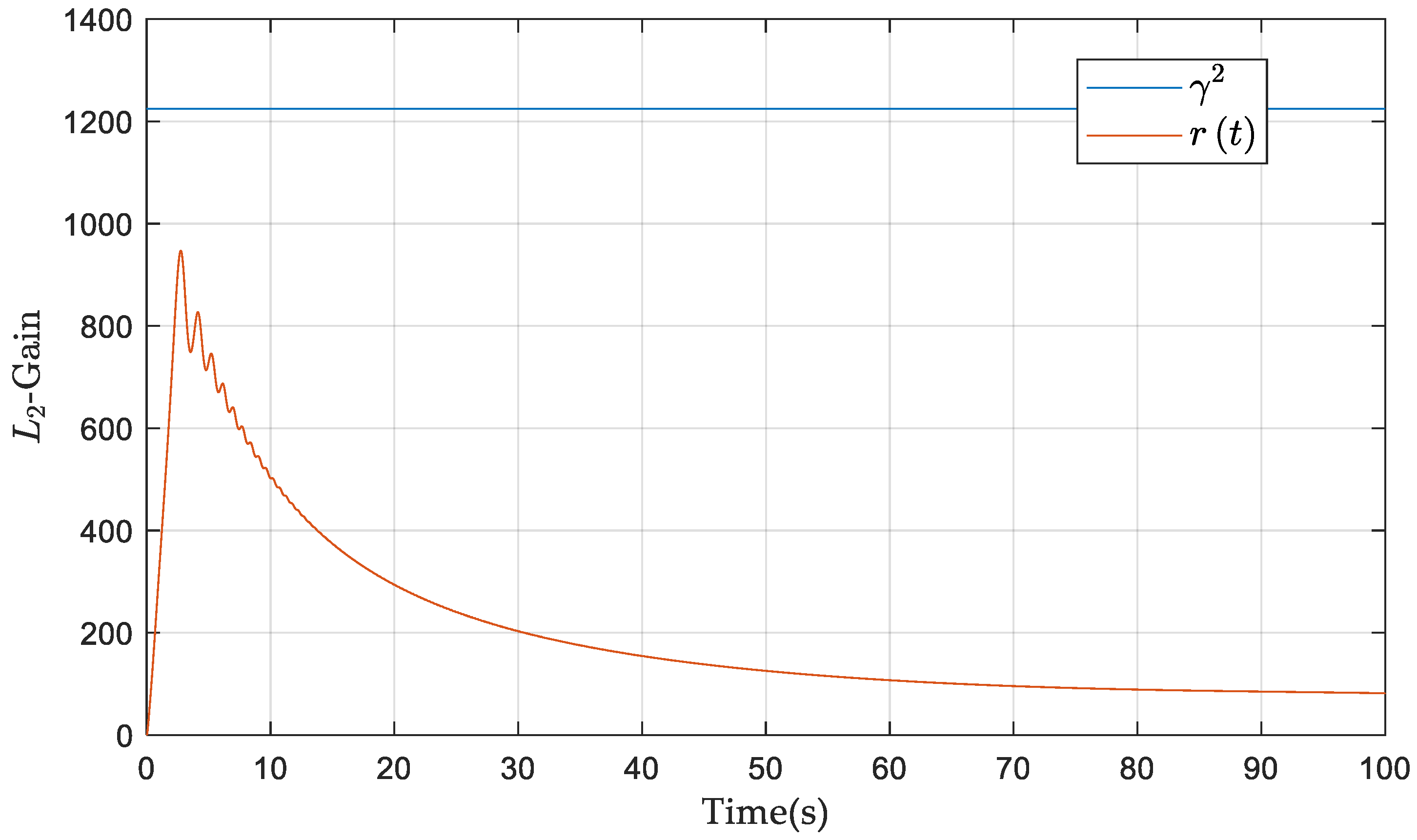
3.1. H_∞ Differential Game

In this section, we design a nonlinear H_∞ controller based on off-policy RL for the established nonlinear active suspension state-space Equation (5). The road and the controller are considered as two independent players; thus, the design of the H_∞ controller can be transformed into an H_∞ differential game.

First, define the cost function as follows:

$$\begin{array}{l}J\left(x\left(0\right),\hspace{0.33em}u,\hspace{0.33em}\omega \right)\\ ={\displaystyle {\int }_0^{\infty }\left(x^{T}Qx+u^{T}Ru-{\gamma }^2{‖\omega ‖}^2\right)}dt\end{array}$$

(8)

where $Q$ and $R$ are positive definite matrices, and $\gamma$ is a positive constant. $Q$ and $R$ are also the weight matrices of the cost function and are closely related to the performance metrics (6). Under zero initial conditions, if $J\left(x\left(0\right),\hspace{0.33em}u,\hspace{0.33em}\omega \right)\le 0$, then the system has an H_∞ performance, and $\gamma$ is called the disturbance attenuation level.

Define the value function of the H_∞ differential game as

$$\begin{array}{l}V\left(x\left(t\right)\right)\\ ={\displaystyle {\int }_t^{\infty }\left(x^{T}Qx+u^{T}Ru-{\gamma }^2{‖\omega ‖}^2\right)}d\tau \end{array}$$

(9)

Combining Equations (8) and (9), the H_∞ differential game can be expressed as

$$V^{\ast }\left(x\left(t\right)\right)=\underset{u}{\min }\underset{d}{\max }J\left(x\left(0\right),\hspace{0.33em}u,\hspace{0.33em}\omega \right)$$

(10)

where $V^{\ast }\left(x\left(t\right)\right)$ is the optimal value function.

In Equation (10), the control policy $u$ needs to minimize the cost function, while the disturbance policy $\omega$ needs to maximize the cost function. Therefore, there exists the following Nash equilibrium point:

$$\begin{array}{l}{u}^{\ast }=\underset{u}{\arg \min } J\left(x\left(0\right),\hspace{0.33em}u,\hspace{0.33em}\omega \right)\\ {\omega }^{\ast }=\underset{\omega }{\arg \max } J\left(x\left(0\right),\hspace{0.33em}u,\hspace{0.33em}\omega \right)\end{array}$$

(11)

Equation (11) is also referred to as the optimal game policy.

Definition 1.

If inequality (12) holds, the policy pair $\left\{u^{\ast },{\omega }^{\ast }\right\}$ is a Nash equilibrium point for the H_∞ differential game.

$$J\left(x\left(0\right),\hspace{0.33em}{u}^{\ast },\hspace{0.33em}\omega \right)\le J\left(x\left(0\right),\hspace{0.33em}{u}^{\ast },\hspace{0.33em}{\omega }^{\ast }\right)\le J\left(x\left(0\right),\hspace{0.33em}u,\hspace{0.33em}{\omega }^{\ast }\right)$$

(12)

To find the Nash equilibrium point of the H_∞ differential game, first establish the Hamilton–Jacobi–Isaacs (HJI) equation for the active suspension. By differentiating the value function (9), we get

$$\begin{array}{l}{x}^{T}Qx+u^{T}Ru-{\gamma }^2{‖\omega ‖}^2\\ +\nabla V^T\left(A\left(x\right)+B\left(x\right)u+C\omega \right)=0\end{array}$$

(13)

where $\nabla V=\partial V/\partial x$. Equation (13) is called the Bellman equation, and solving this partial differential equation yields the value function $V\left(x\right)$.

Define the Hamiltonian function of Equation (13) as

$$\begin{array}{l}H\left(x,\nabla V,u,\omega \right)\\ =x^{T}Qx+u^{T}Ru-{\gamma }^2{‖\omega ‖}^2\\ +\nabla V^T\left(A\left(x\right)+B\left(x\right)u+C\omega \right)\end{array}$$

(14)

Based on the static condition of (14), ${\displaystyle \frac{\partial H}{\partial u}}=0$ and ${\displaystyle \frac{\partial H}{\partial \omega }}=0$, the Nash equilibrium point of the H_∞ differential game can be obtained as [1–1]

$$\begin{array}{l}{u}^{\ast }=u^{\ast }\left(V\left(x\right)\right)=-{\displaystyle \frac{1}{2}}{R}^{-1}B{\left(x\right)}^T\nabla V\\ {\omega }^{\ast }={\omega }^{\ast }\left(V\left(x\right)\right)={\displaystyle \frac{1}{2{\gamma }^2}}{C}^T\nabla V\end{array}$$

(15)

Equation (15) is the saddle point of the Hamiltonian function, and substituting it into Equation (13) yields the HJI equation

$$\begin{array}{l}{x}^{T}Qx+{\displaystyle \frac{1}{4}}\nabla V^{T}B\left(x\right)R^{-1}B{\left(x\right)}^T\nabla V-{\displaystyle \frac{1}{4{\gamma }^2}}\nabla V^{T}C{C}^T\nabla V\\ +\nabla V^T\left(A\left(x\right)-{\displaystyle \frac{1}{2}}B\left(x\right)R^{-1}B{\left(x\right)}^T\nabla V+{\displaystyle \frac{1}{2{\gamma }^2}}C{C}^T\nabla V\right)=0\end{array}$$

(16)

The analytical solution of (16) is the optimal value function $V^{\ast }\left(x\left(t\right)\right)$, and $V^{\ast }\left(x\left(t\right)\right)$ satisfies the positive semi-definite condition.

From the above analysis, it is evident that solving the HJI equation can yield the optimal value function and the optimal game policies. Substituting the analytical solution back into Equation (14) gives $H\left(x,\nabla V^{\ast },u^{\ast },{\omega }^{\ast }\right)=0$. However, directly solving the HJI equation is extremely difficult. This paper will design a method based on off-policy RL for approximate solutions.

Theorem 1.

If a positive semi-definite solution $V^{\ast }\left(x\left(t\right)\right)$ exists for the HJI Equation (16), then$\left\{u^{\ast },{\omega }^{\ast }\right\}$ satisfies the following conditions: (1) For all $\omega \in L_2\left[0,\infty \right]$, the half-car active suspension closed-loop system (5) under zero initial conditions meets H_∞ performance and is asymptotically stable in the absence of disturbances; (2) $\left\{u^{\ast },{\omega }^{\ast }\right\}$ is the Nash equilibrium of the H_∞ differential game.

Proof. 

Since $V^{\ast }\left(x\left(t\right)\right)\ge 0$ is a solution of the HJI equation and $V^{\ast }\left(x\right)=0$ with $x=0$, we choose $V\left(x\left(t\right)\right)$ as the Lyapunov function. Differentiating it, we obtain

$$\begin{array}{l}\dot{V}\left(x\right)\\ =\nabla V^T\left(A\left(x\right)+B\left(x\right)u+C\omega \right)\\ =-\left(x^{T}Qx+u^{T}Ru-{\gamma }^2{‖\omega ‖}^2\right)\end{array}$$

(17)

Clearly, combining Equation (17) with Equation (15), we obtain

$$\begin{array}{l}\nabla V^T\left(A\left(x\right)+B\left(x\right)u+C\omega \right)\\ +\left(x^{T}Qx+u^{T}Ru-{\gamma }^2{‖\omega ‖}^2\right)\\ =H\left(x,\nabla V,u,\omega \right)\\ =H\left(x,\nabla V,u^{\ast },{\omega }^{\ast }\right)+{\left(u-u^{\ast }\right)}^{T}R\left(u-u^{\ast }\right)\\ -{\gamma }^2{\left(\omega -{\omega }^{\ast }\right)}^T\left(\omega -{\omega }^{\ast }\right)\end{array}$$

(18)

If $u=u^{\ast }$ and $V=V^{\ast }$, then Equation (18) satisfies the condition

$$H\left(x,\nabla V^{\ast },u^{\ast },\omega \right)=-{\gamma }^2{\left(\omega -{\omega }^{\ast }\right)}^T\left(\omega -{\omega }^{\ast }\right)\le 0$$

(19)

Further integrating Equation (17) gives

$$\begin{array}{l}{V}^{\ast }\left(x\left(T\right)\right)-V^{\ast }\left(x\left(0\right)\right)\\ \le -{\displaystyle {\int }_0^T\left(x^{T}Qx+{u^{\ast }}^{T}R{u}^{\ast }-{\gamma }^2{‖\omega ‖}^2\right)d\tau }\end{array}$$

(20)

Since $V^{\ast }\left(x\left(0\right)\right)=0$ and $V^{\ast }\left(x\left(T\right)\right)\ge 0$, the closed-loop system satisfies H_∞ performance under zero initial conditions as

$${\displaystyle {\int }_0^T\left(x^{T}Qx+{u^{\ast }}^{T}R{u}^{\ast }\right)d\tau }\le {\displaystyle {\int }_0^T{\gamma }^2{‖\omega ‖}^{2}d\tau },\forall \omega \in L_2\left[0,\infty \right]$$

(21)

Note that when $\omega =0$, Equation (17) satisfies ${\dot{V}}^{\ast }\left(x\right)\le 0$, indicating asymptotic stability of the closed-loop system in the absence of disturbances.

To prove that $\left\{u^{\ast },{\omega }^{\ast }\right\}$ is a Nash equilibrium point of the H_∞ differential game, rewrite the cost function (8) as

$$\begin{array}{l}J\left(x\left(0\right),\hspace{0.33em}u,\hspace{0.33em}\omega \right)\\ ={\displaystyle {\int }_0^{\infty }\left(x^{T}Qx+u^{T}Ru-{\gamma }^2{‖\omega ‖}^2\right)}dt\\ +{\displaystyle {\int }_0^{\infty }\dot{V}}dt-V\left(x\left(\infty \right)\right)+V\left(x\left(0\right)\right)\\ ={\displaystyle {\int }_0^{\infty }H}\left(x,\nabla V,u,\omega \right)dt-V\left(x\left(\infty \right)\right)+V\left(x\left(0\right)\right)\end{array}$$

(22)

Considering $t\to \infty$ and $V\left(x\left(\infty \right)\right)\to 0$, we have

$$\begin{array}{l}J\left(x\left(0\right),\hspace{0.33em}u,\hspace{0.33em}\omega \right)\\ ={\displaystyle {\int }_0^{\infty }H}\left(x,\nabla V,u^{\ast },{\omega }^{\ast }\right)dt+V\left(x\left(0\right)\right)\\ +{\displaystyle {\int }_0^{\infty }\left[{\left(u-u^{\ast }\right)}^{T}R\left(u-u^{\ast }\right)-{\gamma }^2{\left(\omega -{\omega }^{\ast }\right)}^T\left(\omega -{\omega }^{\ast }\right)\right]}dt\end{array}$$

(23)

Let $V\left(x\right)=V^{\ast }\left(x\right)$, and from (23) we obtain inequality (12). According to Definition 1, $\left\{u^{\ast },{\omega }^{\ast }\right\}$ is indeed a Nash equilibrium point of the H_∞ differential game. Thus, the proof is complete. □

3.2. Off-Policy RL Algorithm

To solve the HJI Equation (16) numerically, this section designs an off-policy RL algorithm. Compared to on-policy RL algorithms, off-policy methods do not require real-time updates, making them safer as they do not affect the actual physical system. Additionally, this method does not require any model parameter information, which can reduce design costs. The algorithm structure is illustrated in Figure 2. In Figure 2, the state data of the active suspension during the vehicle’s operation is first collected as input. The actor and critic neural networks are then employed to learn the solution to the integral Bellman equation online, with the neural network (NN) weights being continuously updated until convergence is achieved. A portion of the active suspension vibration data is extracted and used to update the value function, control policy, and disturbance policy in real time within an actor–critic RL framework.

Firstly, rewrite the nonlinear state-space equations of the active suspension as

$$\begin{array}{l}\dot{x}=A\left(x\right)+B\left(x\right)u_k+C{\omega }_k\\ +B\left(x\right)\left(u-u_k\right)+C\left(\omega -{\omega }_k\right)\end{array}$$

(24)

where $u$ and $\omega$ are arbitrary but reasonable control inputs and road disturbances, and $u_k$ and ${\omega }_k$ are the control and disturbance policies to be updated.

Combining (15) and (24), differentiating the value function (9) yields

$$\begin{array}{l}{\dot{V}}_k\left(x\right)\\ =\nabla {V_k}^T\left(A\left(x\right)+B\left(x\right)u_k+C{\omega }_k\right)\\ +\nabla {V_k}^T\left(B\left(x\right)\left(u-u_k\right)+C\left(\omega -{\omega }_k\right)\right)\\ =-\left(x^{T}Qx+{u_k}^{T}R{u}_k-{\gamma }^2{‖{\omega }_k‖}^2\right)\\ -2{u_{k+1}}^{T}R\left(u-u_k\right)+\nabla {V_k}^{T}C\left(\omega -{\omega }_k\right)\end{array}$$

(25)

Integrating (25) yields

$$\begin{array}{l}{\left.V_k\right|}_{x\left(t\right)}^{x\left(t+T\right)}=\\ -{\displaystyle {\int }_t^{t+T}\left(x^{T}Qx+{u_k}^{T}R{u}_k-{\gamma }^2{‖{\omega }_k‖}^2\right)d\tau }\\ -{\displaystyle {\int }_t^{t+T}2{u_{k+1}}^{T}R\left(u-u_k\right)}d\tau \\ +{\displaystyle {\int }_t^{t+T}\nabla {V_k}^{T}C\left(\omega -{\omega }_k\right)}d\tau \end{array}$$

(26)

In Equation (26), to simultaneously solve for $V_k$ and $u_{k+1}$, define the actor NN and critic NN as follows:

$$\begin{array}{l}{u}_{k+1}\left(x\right)={\mathsf{\Theta }}_{k+1}^T\sigma \left(x\right)\\ V_k\left(x\right)=W_k^T\varphi \left(x\right)\end{array}$$

(27)

where $\sigma \left(x\right)\in {\Re }^{\alpha }$ and $\varphi \left(x\right)\in {\Re }^{\beta }$ are the basis functions of the NNs, and ${\mathsf{\Theta }}_{k+1}^T$ and $W_k^T$ are appropriate weight coefficients.

Substituting (27) into (26) gives

$$\begin{array}{l}{\left.W_k^T\varphi \left(x\right)\right|}_{x\left(t\right)}^{x\left(t+T\right)}=\\ -{\displaystyle {\int }_t^{t+T}\left(x^{T}Qx+{u_k}^{T}R{u}_k-{\gamma }^2{‖{\omega }_k‖}^2\right)d\tau }\\ -{\displaystyle {\int }_t^{t+T}2\sigma {\left(x\right)}^T{\mathsf{\Theta }}_{k+1}R\left(u-u_k\right)}d\tau \\ +{\displaystyle {\int }_t^{t+T}{W}_k^T\left[\begin{array}{cccc}\frac{\partial \varphi \left(x\right)}{\partial x_1}& \frac{\partial \varphi \left(x\right)}{\partial x_2}& \cdots & \frac{\partial \varphi \left(x\right)}{\partial x_8}\end{array}\right]C\left(\omega -{\omega }_k\right)}d\tau \end{array}$$

(28)

From Equation (28), it can be seen that the NN weight coefficients can be solved offline without the need for model parameters. To ensure the uniqueness of solution in Equation (28), define

$${\left.\xi \left(t\right)=\varphi {\left(x\right)}^T\right|}_{x\left(t\right)}^{x\left(t+T\right)}-{\displaystyle {\int }_t^{t+T}{\left(\omega -{\omega }_k\right)}^T{C}^T{\left[\begin{array}{cccc}\frac{\partial \varphi \left(x\right)}{\partial x_1}& \frac{\partial \varphi \left(x\right)}{\partial x_2}& \cdots & \frac{\partial \varphi \left(x\right)}{\partial x_8}\end{array}\right]}^T}d\tau$$

(29)

$$\zeta \left(t\right)={\displaystyle {\int }_t^{t+T}2{\left(u-u_k\right)}^T{R}^T\otimes \sigma {\left(x\right)}^T}d\tau$$

(30)

$$\varsigma \left(t\right)=-{\displaystyle {\int }_t^{t+T}\left(x^{T}Qx+{u_k}^{T}R{u}_k-{\gamma }^2{‖{\omega }_k‖}^2\right)d\tau }$$

(31)

where

$$\begin{array}{l}t=t_{k,1},t_{k,2},\cdots t_{k,𝓁}\\ 0\le t_{k,i}+T\le t_{k,i+1}\\ t_{k,i}+T\le t_{k+1,1},k=0,1,\cdots \infty ,i=1,2,\cdots 𝓁\end{array}$$

Combining (29)–(31), Equation (28) can be rewritten compactly as the following equation:

$${\mathsf{\Phi }}_k\cdot {\mathsf{\Xi }}_k={\mathsf{\Omega }}_k$$

(32)

where

$${\mathsf{\Phi }}_k=\left[\begin{array}{cc}\xi \left(t_{k,1}\right)& \zeta \left(t_{k,1}\right)\\ \xi \left(t_{k,2}\right)& \zeta \left(t_{k,2}\right)\\ ⋮& ⋮\\ \xi \left(t_{k,𝓁}\right)& \zeta \left(t_{k,𝓁}\right)\end{array}\right],{\mathsf{\Xi }}_k=\left[\begin{array}{c}vec\left(W_k\right)\\ vec\left({\mathsf{\Theta }}_{k+1}\right)\end{array}\right],{\mathsf{\Omega }}_k=\left[\begin{array}{c}\varsigma \left(t_{k,1}\right)\\ \varsigma \left(t_{k,2}\right)\\ ⋮\\ \varsigma \left(t_{k,𝓁}\right)\end{array}\right]$$

To ensure Equation (32) has a unique solution, it is necessary to satisfy

$$rank\left({\mathsf{\Phi }}_k\right)\ge \alpha +\beta$$

(33)

where $𝓁\ge \alpha +\beta$ is the dimension of the data, and $\alpha$ and $\beta$ are the dimensions of the basis functions of the actor NN and critic NN, respectively. Thus, the off-policy RL algorithm (Algorithm 1) can be summarized as follows:

Algorithm 1. Off-policy RL algorithm for nonlinear active suspension H∞ differential game.

Step 1: set $k=1$, initialize parameters ${\mathsf{\Theta }}_1$ and $W_0$, apply any reachable $u$ and $\omega$, and collect data $x_1\cdots x_{𝓁}$;

Step 2: Solve the Equation (32) to obtain NN weight coefficients ${\mathsf{\Theta }}_{k+1}^T$ and $W_k^T$ if the Equation (33) holds;

Step 3: Update the actor $u_{k+1}$, ${\omega }_{k+1}$ and critic $V_k$ using (15) and (27);

Step 4: Set $k=k+1$, repeat steps 2–3 until $‖{\mathsf{\Xi }}_k-{\mathsf{\Xi }}_{k-1}‖\le \epsilon$ ($\epsilon$ is a small positive number).

4. Numerical Simulation

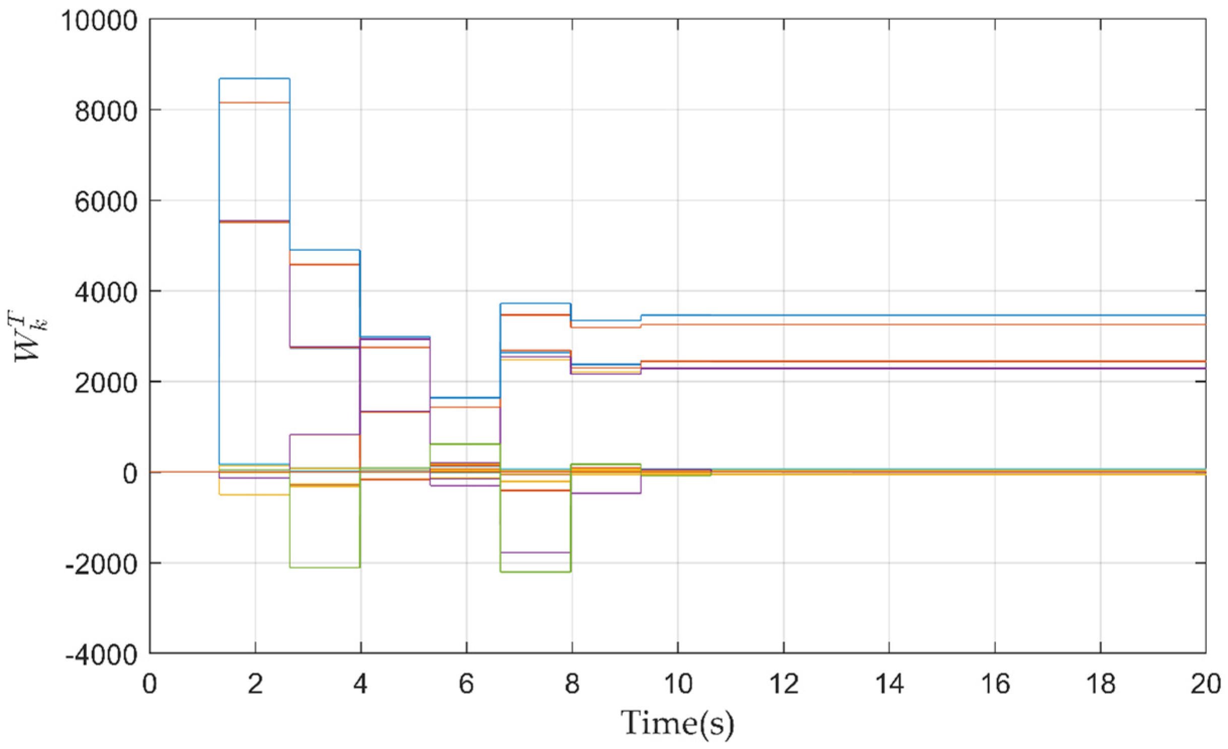
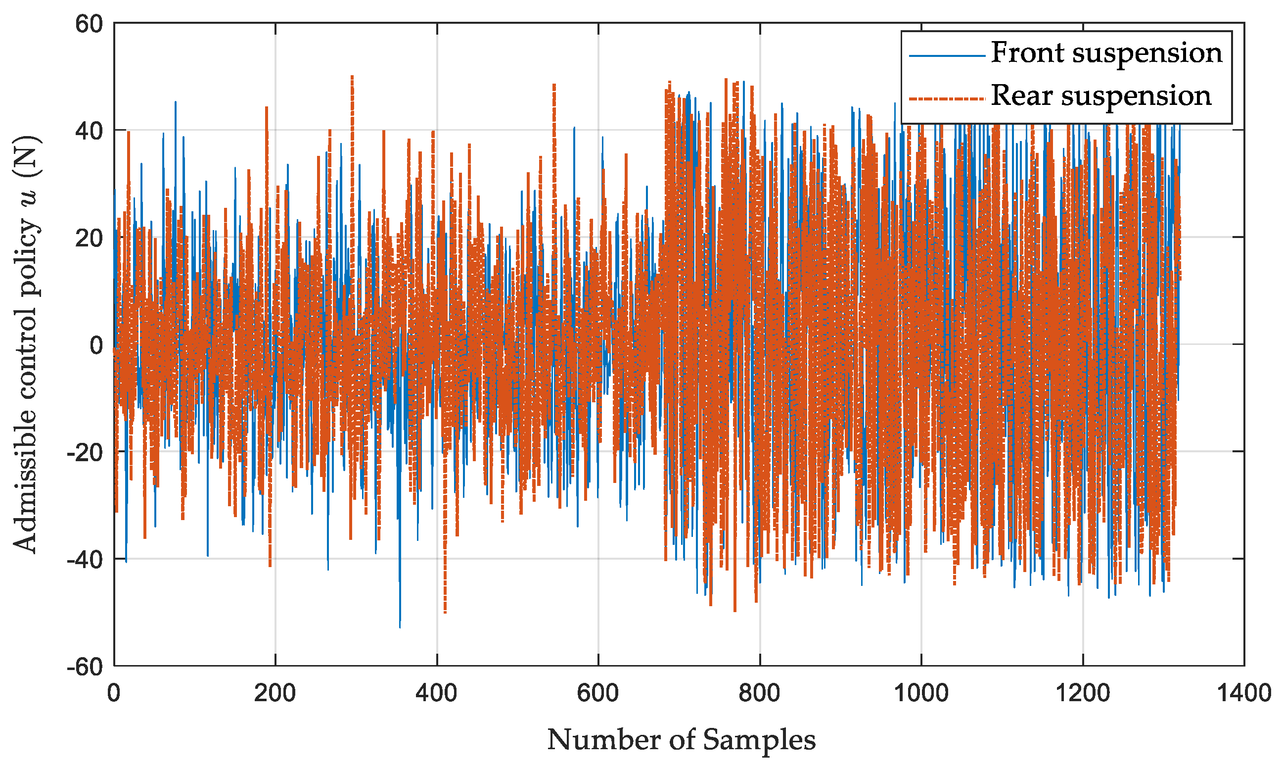
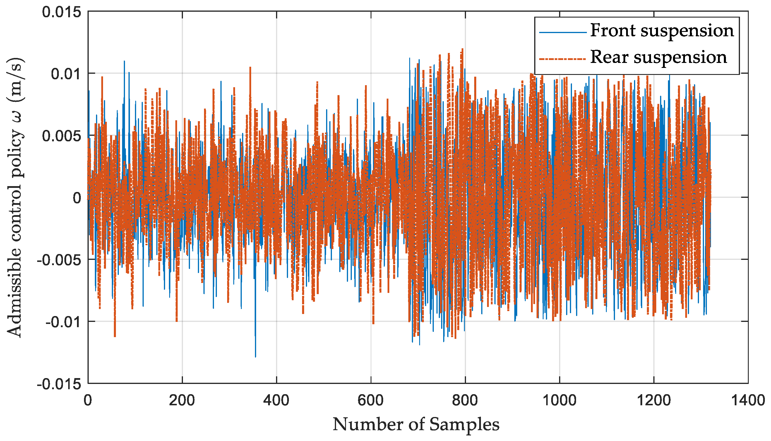
4.1. Implementation of Algorithm 1

To validate the feasibility of the off-policy RL algorithm for the nonlinear active suspension differential game, this section applies Algorithm 1 for policy optimization. The simulation setup uses a hardware-in-the-loop platform, as depicted in Figure 3. The nonlinear active suspension model runs on the MicroAutoBox II, while Algorithm 1 operates on the Speedgoat Controller. The MicroAutoBox II was purchased from the German company dSPACE. The Speedgoat Controller was purchased from Speedgoat in Bern, Switzerland. The MicroAutoBox II is equipped with an IBM PPC 750GL processor (900 MHz), and the Speedgoat Controller features an Intel Celeron 2 GHz CPU with four cores. Real-time data are displayed on the host computer, and the Simulink program runs concurrently.

During the simulation process, the parameters of the vehicle active suspension are listed in

Table 2. Model parameters.

Parameter	Value	Parameter	Value
$M\left(\mathrm{kg}\right)$	500	$a\left(\mathrm{m}\right)$	1.25
$J\left(\mathrm{kg}\cdot {\mathrm{m}}^2\right)$	910	$b\left(\mathrm{m}\right)$	1.45
$m_{t1}\left(\mathrm{kg}\right)$	30	$k_{s1}\left(\mathrm{N}/\mathrm{m}\right)$	10,000
$m_{t2}\left(\mathrm{kg}\right)$	40	$k_{s2}\left(\mathrm{N}/\mathrm{m}\right)$	10,000
$k_{sn1}\left(\mathrm{N}/{\mathrm{m}}^2\right)$	1000	$k_{sn3}\left(\mathrm{N}/{\mathrm{m}}^2\right)$	1000
$k_{sn2}\left(\mathrm{N}/{\mathrm{m}}^3\right)$	20,000	$k_{sn4}\left(\mathrm{N}/{\mathrm{m}}^3\right)$	20,000
$b_{s1}\left(\mathrm{Ns}/\mathrm{m}\right)$	1000	$b_{s2}\left(\mathrm{Ns}/\mathrm{m}\right)$	1000
$k_{t1}\left(\mathrm{N}/\mathrm{m}\right)$	100,000	$u_{1\max }\left(\mathrm{N}\right)$	2000
$k_{t2}\left(\mathrm{N}/\mathrm{m}\right)$	100,000	$u_{2\max }\left(\mathrm{N}\right)$	2000
$z_{1\max }\left(\mathrm{m}\right)$	0.1	$b_{sn1}\left({\mathrm{Ns}}^2/{\mathrm{m}}^2\right)$	200
$z_{2\max }\left(\mathrm{m}\right)$	0.1	$b_{sn2}\left({\mathrm{Ns}}^2/{\mathrm{m}}^2\right)$	200

. The simulation parameters for Algorithm 1 are set as follows: $T=0.01 \mathrm{s}$, $𝓁=132$, $\epsilon =1$, $Q=\mathrm{diag}\left(\right[10,10,10,10,1000,1000,10,10\left]\right)$, $R=0.00001\times \mathrm{eye}\left(2\right)$, $\gamma =35$. All other parameters are set to zero. The NN basis functions are defined as

$$\begin{array}{l}\varphi \left(x\right)={\left[\begin{array}{l}{x}_1^2,2x_1{x}_2,2x_1{x}_3,2x_1{x}_4,2x_1{x}_5,2x_1{x}_6,2x_1{x}_7,2x_1{x}_8,x_2^2,2x_2{x}_3,2x_2{x}_4,2x_2{x}_5,2x_2{x}_6,2x_2{x}_7,2x_2{x}_8,\\ x_3^2,2x_3{x}_4,2x_3{x}_5,2x_3{x}_6,2x_3{x}_7,2x_3{x}_8,x_4^2,2x_4{x}_5,2x_4{x}_6,2x_4{x}_7,2x_4{x}_8,x_5^2,2x_5{x}_6,2x_5{x}_7,2x_5{x}_8,\\ x_6^2,2x_6{x}_7,2x_6{x}_8,x_7^2,2x_7{x}_8,x_8^2,x_1^3,x_2^3,x_3^3,x_4^3,x_5^3,x_6^3,x_7^3,x_8^3\end{array}\right]}^T\\ \sigma \left(x\right)={\left[\begin{array}{l}{x}_1,x_2,x_3,x_4,x_5,x_6,x_7,x_8,x_1^2,2x_1{x}_2,2x_1{x}_3,2x_1{x}_4,2x_1{x}_5,2x_1{x}_6,2x_1{x}_7,2x_1{x}_8,x_2^2,\\ 2x_2{x}_3,2x_2{x}_4,2x_2{x}_5,2x_2{x}_6,2x_2{x}_7,2x_2{x}_8,x_3^2,2x_3{x}_4,2x_3{x}_5,2x_3{x}_6,2x_3{x}_7,2x_3{x}_8,x_4^2,\\ 2x_4{x}_5,2x_4{x}_6,2x_4{x}_7,2x_4{x}_8,x_5^2,2x_5{x}_6,2x_5{x}_7,2x_5{x}_8,x_6^2,2x_6{x}_7,2x_6{x}_8,x_7^2,2x_7{x}_8,x_8^2\end{array}\right]}^T\end{array}$$

The simulation results are shown in Figure 4, Figure 5, Figure 6, Figure 7 and Figure 8. Figure 4 displays the training results of the critic NN weight coefficients, Figure 5 shows the training results of the actor NN weight coefficients, and Figure 6 illustrates the number of policy updates. It can be observed from the figures that the convergence condition is met after 10 updates. Given the sampling time of 0.01 s, the total update time amounts to 13.2 s. Notably, the control and disturbance inputs required for data collection are random white noise signals, which do not necessitate a specific functional form, thereby offering greater applicability. Figure 7 and Figure 8 illustrate the control and disturbance inputs during the data collection process, demonstrating that small inputs are sufficient to meet the requirements. This method ensures the safety of real vehicle data collection.

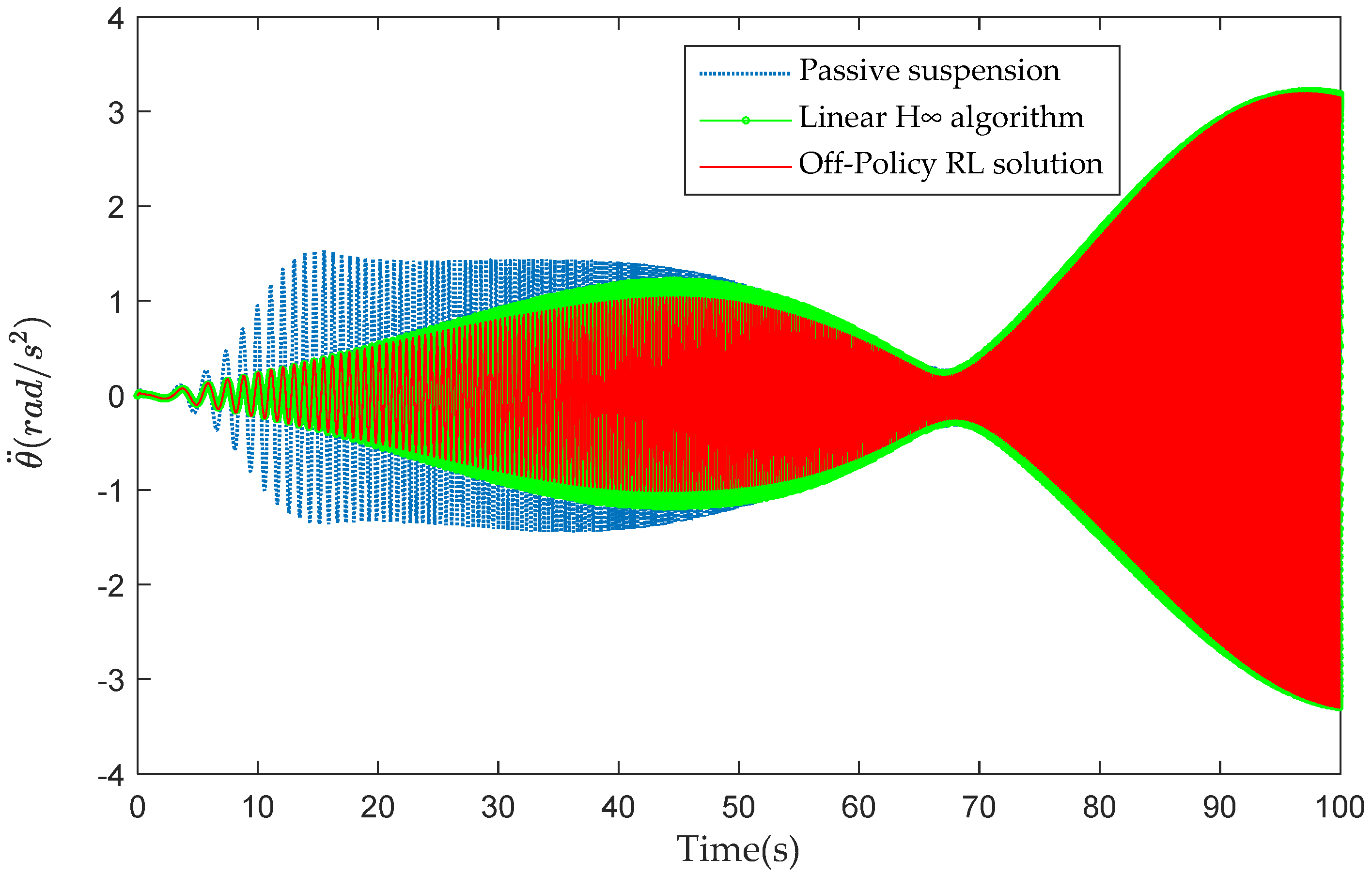
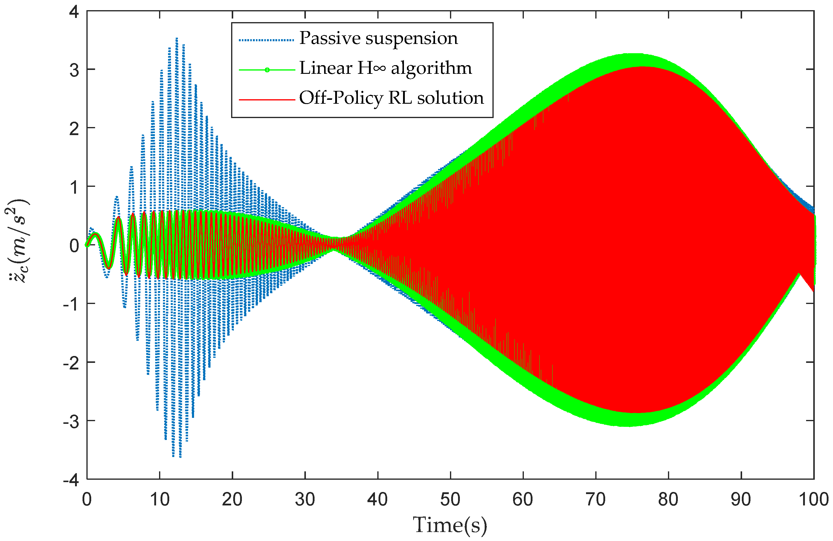
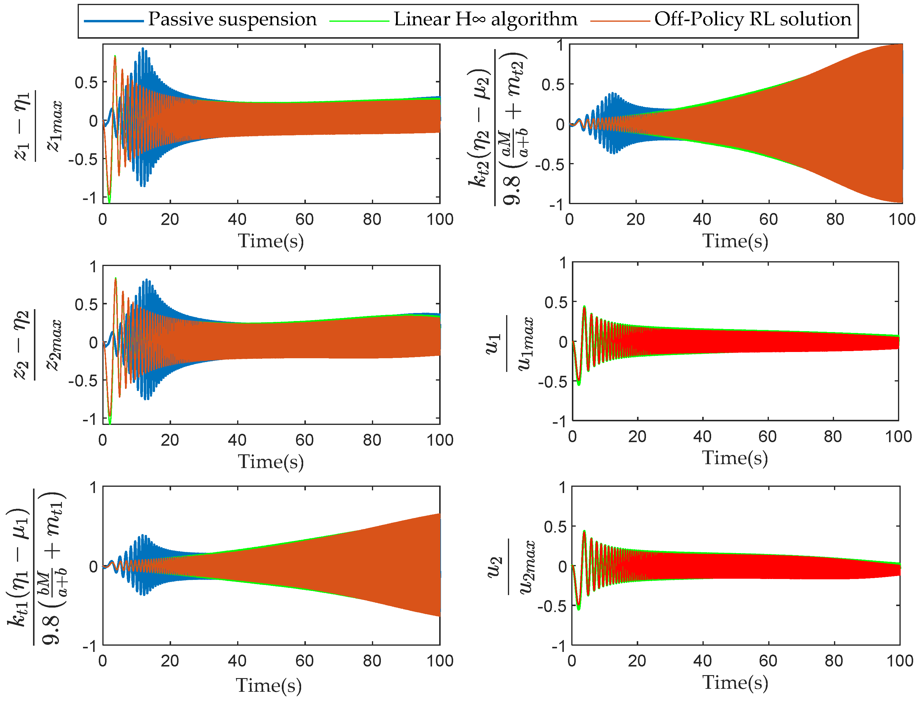
4.2. Vibration Control Performance Analysis

To further verify the effectiveness of the trained control policies, simulations are conducted using a road impact model (7). The vehicle speed is set to $\upsilon =0.36~108 \mathrm{km}/\mathrm{h}$, $L=5 \mathrm{m}$, corresponding to a frequency range from 0.1 Hz to 8 Hz, covering typical road conditions. The simulation results are depicted in Figure 9, Figure 10, Figure 11, Figure 12 and Figure 13. The classic linear H_∞ algorithm [23,27,28] is compared.

Figure 9 shows the road excitation profile, Figure 10 displays the pitch acceleration of the vehicle, Figure 11 illustrates the vertical acceleration of the vehicle body, and Figure 12 presents the response of the suspension performance constraints. From Figure 10 and Figure 11, it can be observed that the trained control policies effectively attenuate vibrations in the frequency range of 0.1–6 Hz, corresponding to vehicle speeds below $80 \mathrm{km}/\mathrm{h}$. For intelligent driving vehicles equipped with visual sensors, vehicle speed can be controlled and planned according to road conditions [1]. Figure 10 and Figure 11 show that, in terms of ride comfort, the off-policy RL solution outperforms traditional linear H_∞ algorithm and passive suspension system. This advantage arises from the method’s ability to account for system nonlinearities, resulting in more effective control performance. Notably, this method requires no model information. Figure 12 indicates that the suspension travel index of the linear H_∞ algorithm exceeds the maximum limit, whereas the proposed method consistently remains within a reasonable range. Additionally, Figure 12 demonstrates that all constraint indicators of the proposed method are less than 1, thereby satisfying the physical constraints during actual driving conditions.

To quantitatively evaluate the simulation results,

Table 3. RMS evaluation of simulation results.

Method	${\ddot{\mathit{z}}}_{\mathit{c}}$(m/s2)	$\ddot{\mathit{\theta }}$(rad/s2)	${\mathit{u}}_1$(N)	${\mathit{u}}_2$(N)
Passive suspension	1.371	1.081	——	——
Linear H∞ algorithm	1.228	1.004	253.6	255.1
Off-Policy RL solution	1.131	0.964	247.2	249.2

presents the root mean square (RMS) values for ${\mathsf{\Lambda }}_1$ and $u$. As shown in Table 3, the off-policy RL solution achieves smaller RMS values, whereas traditional linear H_∞ algorithms, which do not account for nonlinearities, exhibit deviations in control performance.

Table 4. Peak evaluation of simulation results.

Method	${\mathsf{\Lambda }}_2$(1)	${\mathsf{\Lambda }}_2$(2)	${\mathsf{\Lambda }}_2$(3)	${\mathsf{\Lambda }}_2$(4)	${\mathsf{\Lambda }}_2$(5)	${\mathsf{\Lambda }}_2$(6)
Passive suspension	0.9301	0.8131	0.5832	0.9135	——	——
Linear H∞ algorithm	1.076	1.082	0.6153	0.899	0.5484	0.5513
Off-Policy RL solution	0.9725	0.9735	0.6514	0.9894	0.4921	0.4928

provides the peak values for ${\mathsf{\Lambda }}_2$. As evident from Table 4, the off-policy RL solution meets the constraint condition, i.e., ${\mathsf{\Lambda }}_2\left(i\right)<1$. In contrast, the linear H_∞ algorithm’s suspension travel index exceeds the constraint value, resulting in a loss of constraint effectiveness. This occurs because the linear H_∞ method does not account for system nonlinearities, leading to certain indicators being uncontrolled.

To further illustrate the H_∞ performance of the closed-loop system, define the function

$$r\left(t\right)={\displaystyle \frac{{\displaystyle {\int }_0^t\left(x^{T}Qx+u^{T}Ru\right)}d\tau }{{\displaystyle {\int }_0^t{‖\omega ‖}^2}d\tau }}$$

(34)

Figure 13 shows the response of $r\left(t\right)$, indicating that its value remains consistently below the maximum value ${\gamma }^2$, thereby satisfying the H_∞ performance requirement.

5. Conclusions

This paper investigates the H_∞ differential game problem for nonlinear active suspensions, accounting for both geometric nonlinearity and higher-order nonlinearity of the damping elements in the design scheme. An off-policy RL method utilizing an actor–critic structure is employed to approximate the solution to the HJI equation without requiring any model parameters. The simulation results demonstrate the method’s effectiveness. By extracting a portion of the vehicle driving data, the policies can be optimized and converge to the optimal solution after several iterations. Frequency sweep excitation tests reveal that the control policy is effective within the low-frequency range of 0–6 Hz, significantly reducing body vibrations at the first mode while maintaining the physical constraints of the vehicle suspension. Compared to passive suspension and traditional methods, the proposed method reduces vertical acceleration by 20% and 10%, respectively, and pitch acceleration by 10% and 5%. Additionally, the peak control force of the proposed method is 10% smaller than that of traditional methods. All other metrics of the proposed method are below 1, satisfying the time-domain constraints. Future research will explore multi-player collaborative game mechanisms, control saturation constraints, and finite-frequency constraints to further enhance the nonlinear vibration control performance of active suspensions.

References

- Yu, M.; Evangelou, S.A.; Dini, D. Advances in Active Suspension Systems for Road Vehicles. Engineering 2023, 33, 160–177. [Google Scholar] [CrossRef]
- Pan, H.; Zhang, C.; Sun, W. Fault-tolerant multiplayer tracking control for autonomous vehicle via model-free adaptive dynamic programming. IEEE Trans. Reliab. 2022, 72, 1395–1406. [Google Scholar] [CrossRef]
- Li, Q.; Chen, Z.; Song, H.; Dong, Y. Model predictive control for speed-dependent active suspension system with road preview information. Sensors 2024, 24, 2255. [Google Scholar] [CrossRef]
- Zhang, J.; Yang, Y.; Hu, C. An adaptive controller design for nonlinear active air suspension systems with uncertainties. Mathematics 2023, 11, 2626. [Google Scholar] [CrossRef]
- Su, X.; Yang, X.; Shi, P.; Wu, L. Fuzzy control of nonlinear electromagnetic suspension systems. Mechatronics 2014, 24, 328–335. [Google Scholar] [CrossRef]
- Humaidi, A.J.; Sadiq, M.E.; Abdulkareem, A.I.; Ibraheem, I.K.; Azar, A.T. Adaptive backstepping sliding mode control design for vibration suppression of earth-quaked building supported by magneto-rheological damper. J. Low Freq. Noise Vib. Act. Control 2022, 41, 768–783. [Google Scholar] [CrossRef]
- Liu, L.; Sun, M.; Wang, R.; Zhu, C.; Zeng, Q. Finite-Time Neural Control of Stochastic Active Electromagnetic Suspension System with Actuator Failure. IEEE Trans. Intell. Veh. 2024, 1–12. [Google Scholar] [CrossRef]
- Kim, J.; Yim, S. Design of Static Output Feedback Suspension Controllers for Ride Comfort Improvement and Motion Sickness Reduction. Processes 2024, 12, 968. [Google Scholar] [CrossRef]
- Li, P.; Lam, J.; Cheung, K.C. Multi-objective control for active vehicle suspension with wheelbase preview. J. Sound Vib. 2014, 333, 5269–5282. [Google Scholar] [CrossRef]
- Pang, H.; Wang, Y.; Zhang, X.; Xu, Z. Robust state-feedback control design for active suspension system with time-varying input delay and wheelbase preview information. J. Frankl. Inst. 2019, 356, 1899–1923. [Google Scholar] [CrossRef]
- Liu, Z.; Si, Y.; Sun, W. Ride comfort oriented integrated design of preview active suspension control and longitudinal velocity planning. Mech. Syst. Signal Process. 2024, 208, 110992. [Google Scholar] [CrossRef]
- Rodriguez-Guevara, D.; Favela-Contreras, A.; Beltran-Carbajal, F.; Sotelo, C.; Sotelo, D. A Differential Flatness-Based Model Predictive Control Strategy for a Nonlinear Quarter-Car Active Suspension System. Mathematics 2023, 11, 1067. [Google Scholar] [CrossRef]
- Guo, X.; Zhang, J.; Sun, W. Robust saturated fault-tolerant control for active suspension system via partial measurement information. Mech. Syst. Signal Process. 2023, 191, 110116. [Google Scholar] [CrossRef]
- Xue, W.; Li, K.; Chen, Q.; Liu, G. Mixed FTS/H∞ control of vehicle active suspensions with shock road disturbance. Veh. Syst. Dyn. 2019, 57, 841–854. [Google Scholar] [CrossRef]
- Li, H.; Jing, X.; Lam, H.K.; Shi, P. Fuzzy sampled-data control for uncertain vehicle suspension systems. IEEE Trans. Cybern. 2013, 44, 1111–1126. [Google Scholar]
- Sun, W.; Gao, H.; Kaynak, O. Finite frequency H∞ control for vehicle active suspension systems. IEEE Trans. Control Syst. Technol. 2010, 19, 416–422. [Google Scholar] [CrossRef]
- Dogruer, C.U. Constrained model predictive control of a vehicle suspension using Laguerre polynomials. Proc. Inst. Mech. Eng. Part C J. Mech. Eng. Sci. 2020, 234, 1253–1268. [Google Scholar] [CrossRef]
- Esmaeili, J.S.; Akbari, A.; Farnam, A.; Azad, N.L.; Crevecoeur, G. Adaptive Neuro-Fuzzy Control of Active Vehicle Suspension Based on H2 and H∞ Synthesis. Machines 2023, 11, 1022. [Google Scholar] [CrossRef]
- Han, X.; Zhao, X.; Karimi, H.R.; Wang, D.; Zong, G. Adaptive optimal control for unknown constrained nonlinear systems with a novel quasi-model network. IEEE Trans. Neural Netw. Learn. Syst. 2021, 33, 2867–2878. [Google Scholar] [CrossRef]
- Huang, T.; Wang, J.; Pan, H. Approximation-free prespecified time bionic reliable control for vehicle suspension. IEEE Trans. Autom. Sci. Eng. 2023, 1–11. [Google Scholar] [CrossRef]
- Qin, Z.C.; Xin, Y. Data-driven H∞ vibration control design and verification for an active suspension system with unknown pseudo-drift dynamics. Commun. Nonlinear Sci. Numer. Simul. 2023, 125, 107397. [Google Scholar] [CrossRef]
- Mazouchi, M.; Yang, Y.; Modares, H. Data-driven dynamic multiobjective optimal control: An aspiration-satisfying reinforcement learning approach. IEEE Trans. Neural Netw. Learn. Syst. 2021, 33, 6183–6193. [Google Scholar] [CrossRef]
- Wang, G.; Li, K.; Liu, S.; Jing, H. Model-Free H∞ Output Feedback Control of Road Sensing in Vehicle Active Suspension Based on Reinforcement Learning. J. Dyn. Syst. Meas. Control 2023, 145, 061003. [Google Scholar] [CrossRef]
- Wang, A.; Liao, X.; Dong, T. Event-driven optimal control for uncertain nonlinear systems with external disturbance via adaptive dynamic programming. Neurocomputing 2018, 281, 188–195. [Google Scholar] [CrossRef]
- Wu, H.N.; Luo, B. Neural Network Based Online Simultaneous Policy Update Algorithm for Solving the HJI Equation in Nonlinear H∞ Control. IEEE Trans. Neural Netw. Learn. Syst. 2012, 23, 1884–1895. [Google Scholar] [PubMed]
- Luo, B.; Wu, H.N.; Huang, T. Off-policy reinforcement learning for H∞ control design. IEEE Trans. Cybern. 2014, 45, 65–76. [Google Scholar] [CrossRef]
- Kiumarsi, B.; Lewis, F.L.; Jiang, Z.P. H∞ control of linear discrete-time systems: Off-policy reinforcement learning. Automatica 2017, 78, 144–152. [Google Scholar] [CrossRef]
- Wu, H.N.; Luo, B. Simultaneous policy update algorithms for learning the solution of linear continuous-time H∞ state feedback control. Inf. Sci. 2013, 222, 472–485. [Google Scholar] [CrossRef]
- Valadbeigi, A.P.; Sedigh, A.K.; Lewis, F.L. H∞ Static Output-Feedback Control Design for Discrete-Time Systems Using Reinforcement Learning. IEEE Trans. Neural Netw. Learn. Syst. 2019, 31, 396–406. [Google Scholar] [CrossRef]
- Sun, W.; Zhao, Z.; Gao, H. Saturated adaptive robust control for active suspension systems. IEEE Trans. Ind. Electron. 2012, 60, 3889–3896. [Google Scholar] [CrossRef]
- Li, W.; Du, H.; Feng, Z.; Ning, D.; Li, W.; Sun, S.; Tu, L.; Wei, J. Singular system-based approach for active vibration control of vehicle seat suspension. J. Dyn. Syst. Meas. Control 2020, 142, 091003. [Google Scholar] [CrossRef]