Abstract
Graph query languages such as Cypher are widely adopted to match and retrieve data in a graph representation, due to their ability to retrieve and transform information. Even though the most natural way to match and transform information is through rewriting rules, those are scarcely or partially adopted in graph query languages. Their inability to do so has a major impact on the subsequent way the information is structured, as it might then appear more natural to provide major constraints over the data representation to fix the way the information should be represented. On the other hand, recent works are starting to move towards the opposite direction, as the provision of a truly general semistructured model (GSM) allows to both represent all the available data formats (Network-Based, Relational, and Semistructured) as well as support a holistic query language expressing all major queries in such languages. In this paper, we show that the usage of GSM enables the definition of a general rewriting mechanism which can be expressed in current graph query languages only at the cost of adhering the query to the specificity of the underlying data representation. We formalise the proposed query language in terms declarative graph rewriting mechanisms described as a set of production rules while both providing restriction to the characterisation of L, and extending it to support structural graph nesting operations, useful to aggregate similar information around an entry-point of interest. We further achieve our declarative requirements by determining the order in which the data should be rewritten and multiple rules should be applied while ensuring the application of such updates on the GSM database is persisted in subsequent rewriting calls. We discuss how GSM, by fully supporting index-based data representation, allows for a better physical model implementation leveraging the benefits of columnar database storage. Preliminary benchmarks show the scalability of this proposed implementation in comparison with state-of-the-art implementations.
Keywords:
direct acyclic graphs; generalised semistructured model; graph grammars; graph query languages; algorithms; operator algebras MSC:
68W40; 68P15; 68Q42; 68Q55; 68R10; 68U35
1. Introduction
Query languages [1] fulfill the aim of retrieving and manipulating data after being adequately processed according to a physical model requiring preliminary data loading and indexing operations. Good declarative languages for manipulating information, such as SQL [2], are agnostic from the underlying physical model while expressing the information need of combining (JOIN), filtering (WHERE) and grouping (e.g., COUNT(*) over GROUP BY-s) data over its logical representation. This language can also be truly declarative as it does not require a user to explicitly convey this in terms of operations to be performed over the data rather than instructing the machine which information should be used and which types of transformations should be applied. Due to the intrinsic nature of graph data representation, graph query languages such as Gremlin [3], Cypher [4], or SPARQL [5] are procedural (i.e., navigational) due to the navigational structure of the data, thus heavily requiring the user to inform the language how to match and transform the data. These considerations extend to how edge and vertex data should be treated, thus adding further complexity [6,7].
On the other hand, graph grammars [8] provide a high-level declarative way to match specific sub-graphs of interest from vertex-labelled graphs for then rewriting them into another subgraph of interest, thus updating the original graph of interest. These consist in a set of rules , where each rule consists of two graphs and possibly sharing a common subgraph K: while specifies a potential removal of either vertices or edges, specifies their addition. Automating the application of such rules requires explicitly following a graph navigational order for applying each matched subgraph to the structure [9] to guarantee the generation of a unique acceptable graph representation resulting from the querying data. As a by-product of exploiting topological sorts for scheduling visiting and rewriting operations, we then require to precisely identify an entry match vertex for each from a rule, thus precisely determining from which position within the graph the rewriting rule should be applied, and in which order.
At the time of writing, the aforementioned graph query languages are not able to express graph grammars natively without resorting to explicitly instructing the query language how to restructure the underlying graph data representation (Lemma 7); furthermore, the replacement of previously matched vertices with new ones invalidates previous matches, thus forcing the user to pipeline different queries until convergence is reached. On the other hand, we would expect any graph query language to directly express the rewriting mechanism by directly expressing the set of rules, without necessarily instructing the querying language in which order such operations shall be performed. Furthermore, when a property-graph model is chosen, and morphisms are expressed through the properties associated with the vertices and edges rather than their associated IDs as per the current Cypher and Neo4j v5.20 specifications, this makes the deletion of vertices and their update through the resulting morphisms quite impractical, as such data model provides no clear way to refer to both vertices and edges via unique identifiers. As a result of these considerations, we then derive that, at the time of writing, both the graph query languages and their underlying representational model are insufficient to adequately express rewriting rules as general as the ones postulated by graph grammars over graphs containing property-value associations, independently from their representation of choice [10].
To overcome the aforementioned limitations, we propose a query language, for the first time directly expressing such rewriting desiderata: we restrict the set of all the possible matching graphs into ego-nets containing one entry-point while incorporating nesting operations (Section 6.1); as updating graph vertices’ properties breaks the declarative assumption as the user should specify the order in which the operations are performed, we relax the language declarativity for the sole rewritings. To better support this query language, we completely shift the data model of interest to object-oriented databases, where relationships across objects are expressed through object “containment” relationships, and where both objects and such containments are uniquely identified. By also requiring that any object shall never contain itself at any nesting level [6], we obtain cycle-free containment relationships.
The paper is structured as follows: after providing some preliminary notation used throughout the paper (Section 2), we introduce the relational and the graph data models from current literature, while focusing on both their data representation and associated query languages (Section 3). Their juxtaposition motivates the proposal of our Generalised Semistructured Model (Section 4), for which we outline both the logical and physical data model, where the latter leverages state-of-the-art columnar relational database representations [11]; we also introduce the concept of a view for a generalised semistructured model, as well as introduce some morphism notation used throughout the paper. After introducing the designated operator for instantiating the morphisms by joining matched containments stored in distinct sets of tables (Section 5), we finally propose our query language for matching and rewriting object-oriented databases expressed in the aforementioned GSM model (Section 6). We characterise the formal semantics of such novel graph query language in pseudocode notation (Algorithm from Section 6) characterised in terms of both algorithmic and algebraic notation (Section 6.3 and Section 6.4) for the matching part, as well as in terms of Structured Operational Semantics (SOS) [12] for describing the rewriting steps (Section 6.5). The remaining sections discuss some of the expressiveness properties of such query language if compared to Cypher (Section 7), discuss its time complexity (Section 8), and benchmark it against Cypher running over Neo4j v5.20, showing the extreme inefficiency of property graph computational model (Section 9), which are fairly restricted due to the impossibility of conveying a novel single query for any possible graph schema (Lemmas in Section 7). Scalability tests show that our solution outperforms Cypher and Neo4j v5.20, providing the query language standard nearer to the recently proposed GQL, by two orders of magnitude (Section 9.1) while providing a computational throughput being 600 times faster than Neo4j by solving more queries in the same comparable amount of time (Section 9.1). Last, we draw our final conclusions where we propose some future works (Section 10). To improve the paper’s readability, we move some definitions (Appendix A) and the full set of proofs for the Lemmas and Corollaries (Appendix B) to the Appendix.
These main contributions are then obtained in terms of the following ancillary results:
- Definition of a novel nested relational algebra natural equi-join operator for composing nested morphisms, also supporting left outer joins by parameter tuning (Section 5).
- Definition of an object-oriented database view for updating the databases on the fly without the need for heavy restructuring of the loaded and indexed physical model (Section 4.3).
- As the latter view relies on the definition of a logical model extending GSM (Section 4.1), we show that the physical model is isomorphic to an indexed set of GSM databases expressed within the logical model (Lemma 1).
2. Preliminary Notation
We denote sets of cardinality as standard. The power set of any set S is the set of all subsets of S, including the empty set ∅ and S itself. Formally, .
We define a finite function via its graph explicating the association between a value from the domain of f () and a non-NULL codomain value. Using an abuse of notation, we denote the restriction as the evaluation of f over a domain , i.e., . We can also denote where C is the definition of the function over x as . With an abuse of notation, we denote as the cardinality of its domain, i.e., . We say that two functions f and are equivalent, , if and only if they both share the same domain and, for each element of their domain, both functions return the same codomain value, i.e., .
A tuple or indexed set of length is defined as a finite function in where has i as a natural-valued independent variable representing the index of the tuple, and the dependent variable corresponds to the element in the tuple.
A binary relation ℜ on a set A is said to be an equivalence relation if and only if it is reflexive (), symmetric (), and transitive (). Given a set A and an equivalence relationship ℜ, an equivalence class for is the set of all the elements in A that are equivalent to x, i.e., . Given a set A and an equivalence relationship ℜ, the quotient set is the set of all the equivalence classes of A, i.e., . We denote as the equivalence relationship denoting two functions as equivalent if they are equivalent after the same restriction over X, i.e., .
Given a set of all the possible string attributes and a set of all the possible values , a record is defined as a finite function with [13]. Given two records represented as finite functions f and , we denote as the overriding of f by returning for each and otherwise. Given this, we can also denote the graph of a function as . We denote as NULL a void value not representing a sensible value in : using the usual notation in the database area at the cost of committing an abuse of notation, we say that returns NULL if and only if f is not defined over x (i.e., ). We say that a record is empty if no attribute is associated with a value in (i.e., and ).
Higher-Order Functions
Higher-Order Functions (HOFs) are functions that either take one or more functions as arguments or return a function as a result. We provide the definition of some HOFs used in this paper:
- The zipping operator maps n tuples (or records) to a record of tuples (or records) r defined as if and only if all n tuples are defined over i:
- Given a function and a generic collection C, the mapping operator returns a new collection by applying f to each component of C:
- Given a binary predicate p and a collection C, the filter function trims C by restricting it to its values satisfying p:
- Given a binary function , an initial value (accumulator), and a tuple C, the (left) fold operator is a tail-recursive function returning either for an empty tuple, or for a tuple :
- Given a collection of strings C and a separator s, collapse (also referred to as join in programming languages such as Javascript or Python ) returns a single string where all the strings in C are separated by s. Given “^” the usual string concatenation operator, this can be expressed in terms of as follows:When s is a space “␣”, then we can use as a shorthand.
- Given a function and two values and , the update of f so that it will return b for a and will return any other previous value for otherwise is defined as follows:
- Given a (finite) function f and an input value y, the HOF optionally obtaining the value of if and returning z otherwise is defined as:Please observe that we can use this function in combination with Put to set multiple nested functions:
3. Related Works
This section outlines different logical models and query languages for both graph data (Section 3.1.1 and Section 3.1.2) and the nested relational model (Section 3.2.1 and Section 3.2.2), while starting from their mathematical foundations. We then discuss an efficient physical model used for the relational model (Section 3.2.3).
3.1. Graph Data
3.1.1. Logical Model
Direct Acyclic Graphs (DAGs) and Topological Sort
A digraph consists of vertices V and edges E being a subset of . We say that such a graph is weighted if its definition is extended as where is a weight function associating each edge in the graph to a real value. A closed trail is a sequence of distinct edges which edge is such that and if any, and where . We say that a digraph is acyclic if it contains no closed trails consisting of at least one edge, and we refer to it as a Direct Acyclic Graph (DAG).
If we assume that edges in a graph reflect dependency relationships across their vertices, a natural way to determine the visiting order of the vertices is first to sort its vertices topologically [14], thus inducing an operational scheduling order [11]. This requires the underlying graph to be a DAG. Notwithstanding this, any DAG might come with multiple possible valid topological sorts; among these, the scheduling of tasks operations usually prefers visiting the operations bottom-up in a layered way, thus ensuring the operations are always applied starting from the sub-graphs having less structural-refactoring requirements that the higher ones [11].
We say that a topological sort of a DAG is a linear ordering of its vertices in a tuple t with so that for any edge we have i and such that and . Given this linear ordering of the vertices, we can always define a layering algorithm [15] where vertices sharing no mutual interdependencies are placed in the same layer, and where all the vertices appearing in the shallowest layer will be connected by transitive closure to all the vertices in the deeper layers, while the vertices in the deepest layer will share no interconnection with the other vertices in the graph. To do so, we can use Algorithm 1: we use timestamps for determining the layer ID: we associate all vertices with no outgoing edge to the deepest layer 0 (Line 5) and, for all the remaining vertices, we set the vertex to the layer immediately below to the one of the deepest outgoing vertex (Line 9).
| Algorithm 1 Layering DAGs from a vertex topological order in t |
|
When the graph is cyclic, we can use heuristics to approximate the vertex order, such as using the progressive ID associated with the vertices to disambiguate and choose an ordering when required.
Property Graphs
Property graphs [16] represent multigraphs (i.e., digraphs allowing for multiple edges among two distinct vertices) expressing both vertices and edges as multi-labelled records. The usefulness of this data model is remarked by its implementation in almost all recent Graph DBMSs, such as Neo4j [4].
Definition 1
(Property Graph). A property graph [9] is a tuple , where V and E are sets of distinct integer identifiers (, , ). L is a set of labels, A is a set of attributes and U is a set of values. maps each vertex or edge to a set of labels; maps each vertex or edge within the graph and each attribute within A, to a value in U; last, maps each edge to a pair of vertices , where s is the source vertex and t is the target.
Property graphs do not support aggregated values, as values in U cannot contain either vertices or edges, nor U is made to contain a collection of values.
RDF
The Resource Description Framework (RDF) [17] distinguishes resources via Unique Resource Identifiers (URI), be them vertices or edges within a graph; those are linked to their properties or other resources via triples, acting as edges. RDF is commonly used in the semantic web and in the ontology field [18,19]. Thus, modern reasoners such as Jena [20] or Pellet [21] assume such data structure as the default graph data model.
Definition 2 (RDF (Graph Data) Model).
An RDF (Graph data) model [9] is defined as a set of triples , where s is called “subject”, p is the “predicate” and o is the “object”. Such triple describes an edge with label p linking the source vertex s to the destination vertex o. Such predicate can also be a source vertex [10]. Each vertex is either identified by a unique URI identifier or by a blank vertex . Each predicate is only described by a URI identifier.
Despite this model using unique resource identifiers for either vertices or edges differently from property graphs, RDF is forced to express attribute-value associations for vertices as additional edges through reification. Thus, property graphs can be entirely expressed as RDF triplestore systems as follows:
Definition 3
(Property Graph over Triplestore). Given a property graph , each vertex induces a set of triples for each such that having . Each edge induces a set of triples such that and another set of triples for each such that having .
The inverse transformation is not always possible as RDF properties as property graphs do not allow the representation of edges departing from other edges. RDF also supports the unique identification of distinct databases being loaded within the same physical storage through named graphs via a resource identifier. Even though it allows named graphs to appear as triplet subjects, such named graphs can appear as neither objects nor properties, thus not overcoming property graphs’ limitations on representing nested data.
Notwithstanding the model’s innate ability to represent both vertices and edges via URIs, the inability of the data model to directly associate each URI with a data record while requiring it to express the property-value associations via triplets, requires the expression of property updates via the deletion and subsequent creation of new triplets of the data, which might be quite impractical. Given all the above, we still focus our attention on the Property Graph model, as it better matches our data representation desiderata by associating to vertices labels, property-value associations, as well as binary relationships without any data duplications.
3.1.2. Query Languages
Despite the recent adoption of a novel graph query language standard, GQL, (https://www.iso.org/obp/ui/en/#!iso:std:76120:en accessed on 19 April 2024), its definition has still to be implemented yet in existing systems. This motivates us to briefly survey currently available languages. Different from the more common characterisation of graph query languages in terms of their potential of expressing traversal queries [22], a better analysis of such languages involves their ability to generate new data. Our previous work [9] proposed the following characterisation:
- Graph Traversal and Pattern Matching: these are mainly navigational languages performing the graph visit through “tractable” algorithms through polynomial time visits with respect to the graph size [18,23,24]. Consequently, such solutions do not necessarily involve running a subgraph isomorphism problem, except when expressly requested by specific semantics [22,25].
- (Simple) Graph Grammars: as discussed in the forthcoming paragraph, they can add and remove new vertices and edges that do not necessarily depend on previously matched data, but they are unable to express full data transformation operations.
- Graph Algebras: these are mainly designed either to change the structure of property graphs through unary operators or to combine them through n-ary (often binary) ones. These are not to be confused with the path-algebras for expressing graph traversal and pattern-matching constructs, as they allow us to completely transform graphs alongside the data associated with them as well as deal with graph data collections [26,27,28,29].
- “Proper” Graph Query Languages: We say that a graph query language is “proper” when its expressive power includes all the aforementioned query languages, and possibly expresses the graph algebraic operators while being able to express, to some extent, graph grammar rewriting rules independently from their ability to express them in a fully-declarative way. This is achieved to some extent in commonly available languages, such as SPARQL and Cypher [4].
Graph Grammars
Graph grammars [30] are the theoretical foundations of current graph query languages, as they express the capability of matching specific patterns L [31] within the data through reachability queries while applying modifications to the underlying graph database structure (graph rewriting) R, thus producing a single graph grammar production rule , where there is an implicit morphism between some of the vertices (and edges) matched in L and the ones appearing in R: the vertices (and edges) only appearing in R are considered as newly inserted vertices, while the vertices (and edges) only appearing in L are considered as removed edges; we preserve the remaining matched vertices. Each rule is then considered as a function f, taking a graph database as an input and returning a transformed graph.
The process of matching L is usually expressed in terms of subgraph isomorphism: given two graphs G and L, we determine whether G contains a subgraph that is isomorphic to L, i.e., there is a bijective correspondence between the vertices and edges of L and . In graph query languages, we consider G as our graph database and return for each matched subgraph . When no rewriting is considered, each possible match for L is usually represented in a tabular form [31,32], where the column header provides the vertex and edge identifiers (e.g., variables) j from L, each row reflects each matched graph , and each cell corresponding to the column j represents . Figure 1 shows the process of querying a graph g (Figure 1a) through a pattern L (Figure 1b), for which all the subgraphs matching in the former could be reported as morphisms listed as rows within a table, which column headers reflect the vertex and edge variables occurring in the graph pattern (Figure 1c).
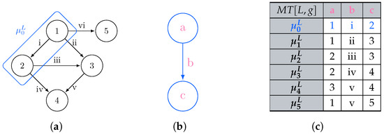
Figure 1.
Listing all the subgraphs of g being a solution of the subgraph isomorphism problem of g over L. (a) Graph g to be mathed; (b) Graph pattern L; (c) Morphism table where each row describes a morphism between the graph matching L and the graph g.
Figure 2 illustrates graph grammar rules as defined in GraphLog [33] for both matching and transforming any graph: we can first create the new vertices required in R, while updating or removing x as determined by the vertex or edge occurring in R. Deletions can be performed as the last operations from R. GraphLog still allows running of one single grammar rule at a time, while authors assume to have a graph where vertices are associated with data values and edges are labelled. Then, the rewriting operations derived from R will be applied to every subgraph being matched via a previously identified morphism in for each graph g of interest. Still, GraphLog considered neither the possibility of simultaneously applying multiple rewriting rules to the same graph nor a formal definition of which order the rules should be applied. The latter is required to ensure that any update on the graph can be performed incrementally while ensuring that any update to a vertex u via th information stored in its neighbours will always rely on the assumption that each neighbour will not be updated in any other subsequent step, thus guaranteeing that the information in u will never become stale.
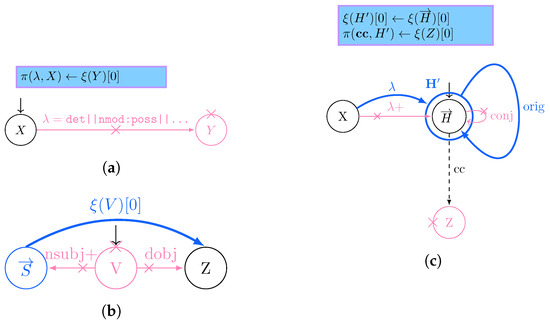
Figure 2.
Graph grammar production rules à la GraphLog [33] in this paper’s use case scenario: thick denotes insertions, crosses deletions, and optional matches are dashed. We extended it with multiple optional edge label matches (‖), key-value association for property and vertex X, and multiple vertex values . (a) Injecting the articles/possessive pronouns () in Y for an entity X as its own properties, while deleting and Y; (b) Expressing the verb as a binary relationship between subject and direct object; (c) Generating a new entity coalescing the ones under the same conjunction Z, while referring to its original constituents via orig.
This paper solves the ordering issue by applying the changes on the vertices according to their inverse topological order, thus updating the vertices sharing the least dependencies with their direct descendants first.
Furthermore, as GraphLog authors are considering a no-property graph model, authors do not consider the possibility of updating multiple property value associations over a vertex, while not providing a formal definition of how aggregation functions over vertex data should be defined. While the first problem can be solved only by properly exploiting a suitable data model, the latter is solved by the combined provision of nested morphism, explicitly nesting the vertices associated with a grouped variable, while exploiting a scripting language for expressing how level data manipulations when strictly required. Given these considerations, we will also discuss graph data models (Section 3.1) and their respective query languages (Section 3.1.2).
Proper Graph Query Languages
Given the above, we will mainly focus our attention on the last type of language. Even though these languages can be closed under either property graphs or RDF, graphs must not be considered as their main output result, since specific keywords like RETURN for Cypher and CONSTRUCT for SPARQL must be used to force the query result to return graphs. Given also the fact that such languages have not been formalised from the graph returning point of view, such languages prove to be quite slow in producing new graph outputs [6,7].
GQL is largely inspired by Cypher, for which this standard might be considered its natural extension. Such query language enables the partial definition of graph grammar operations by supporting the following operators restructuring vertices and edges within the graph: SET, for setting new values within vertices and edges, MERGE, for merging a set of attributes within a single vertex or edges, REMOVE for removing labels and properties from vertices and edges and CREATE for the creating of new vertices, edges and paths.
Notwithstanding the former, such language cannot express all the possible data transformation operations, thus requiring an extension via its APOC library (https://Neo4j.com/developer/Neo4j-apoc/, accessed on 13 November 2023) for defining User-Defined Functions (UDF) in a controlled way, like concatenating the properties associated with vertices’ multiple matches:

Thus, Cypher can collect values for then generating one single vertex (See also Listing A2) but, due to the structural limitations of the query language (not supporting nested morphisms) and data model (not supporting explicit identifiers for both vertices and edges), it does not support the nesting of entire sub-patterns of the original matching.
A further limitation of Cypher is the inability to create a relationship with a variable as the name, as standard Cypher syntax only allows a string parameter. Using the APOC library we can use apoc.create.relationship to pass a variable name from an existing vertex for example. Given our last query creating the vertex x, we can continue the aforementioned query:

As there are no associated formal semantics for the entirety of this language’s operators except its fragment related to graph traversal and matching [16], for our proofs regarding this language (e.g., Lemma 7) we are forced to reduce our arguments to common-sense reasoning an experience-driven observation from the usage of Cypher over Neo4j similarly to the considerations in the former paragraph. In fact, such algebra does not involve the creation of new graphs: this is also reflected by its query evaluation plan, which preferred evaluation is a morphism table rather than expressing the rewriting in terms of updated and resulting property graph. As a result, the process of creating or deleting vertices and edges is not optimised.
Overall, Cypher suffers from the limitations posed by the property graph data model which, by having no direct way to refer to the matched vertices or edges by reference, forces the querying user to always refer to the properties associated with them; as a consequence, the resulting morphism tables are carrying out redundant information that cannot reap the efficient data model posed by columnar databases, where entire records can be referenced by their ID. This is evident for  statements, voiding objects represented within the morphisms. This limitation of the property graph model, jointly with the need for representing acyclic graphs, motivates us to use the Generalised Semistructured Model (GSM) as an underlying data model for representing graphs, thus allowing us to refer to the vertices and edges by their ID [34]. Consequently, our implementation represents morphisms for acyclic property graphs as per Figure 1c.
statements, voiding objects represented within the morphisms. This limitation of the property graph model, jointly with the need for representing acyclic graphs, motivates us to use the Generalised Semistructured Model (GSM) as an underlying data model for representing graphs, thus allowing us to refer to the vertices and edges by their ID [34]. Consequently, our implementation represents morphisms for acyclic property graphs as per Figure 1c. Figure 3a provides a possible property graph instantiation of the digraph originally presented in Figure 1a. Notwithstanding the former definition, Neo4j’s implementation of the Property Graph model substantially differs from the aforementioned mathematical definition, as it does not allow the definition of an explicit resource identifier for both vertices and edges. After expressing the matching query in Figure 1b in Cypher as  *, the resulting morphism table from Figure 3b does not explicitly reference the IDs referring to the specific vertices and edges, thus making it quite impractical to update the values associated with the vertices while continuing to restructure the graph, as this will require to re-match the previously updated data to retain it in the match. Although this issue might be partially solved by exploiting explicit incremental views over the property graph model [32], this solution had no application in Neo4j v5.20, thus making it impossible to fully test its feasibility within the available system. Furthermore, the elimination of an object previously matched within a morphism will update the table by providing an empty object rather than providing a NULL match. This will motivate us to investigate other ID-based graph data models.
*, the resulting morphism table from Figure 3b does not explicitly reference the IDs referring to the specific vertices and edges, thus making it quite impractical to update the values associated with the vertices while continuing to restructure the graph, as this will require to re-match the previously updated data to retain it in the match. Although this issue might be partially solved by exploiting explicit incremental views over the property graph model [32], this solution had no application in Neo4j v5.20, thus making it impossible to fully test its feasibility within the available system. Furthermore, the elimination of an object previously matched within a morphism will update the table by providing an empty object rather than providing a NULL match. This will motivate us to investigate other ID-based graph data models.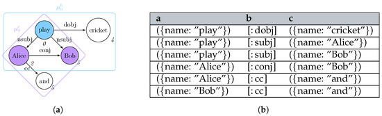
Figure 3.
Framing Figure 1 in the context of Neo4j’s implementation of the Property Graph model. (a) Dependency graph for “Alice and Bob play cricket”; (b) Neo4j’s property graph morphism table.
Neo4j lists some additional existing limitations beyond APOC and the expressibility of graph grammars in a declarative way with Cypher within their documentation (https://Neo4j.com/docs/operations-manual/current/authentication-authorization/limitations/, accessed on 13 November 2023), mainly related to the interplay between data access security requirements and query computations.
At the time of writing, the most studied graph query language both in terms of semantics and expressive power is SPARQL, which allows a specific class of queries that can be sensibly optimised [5,31]. The algebraic language used to formally represent SPARQL performs queries’ incremental evaluations [35], and hence allows for boosting the querying process while data undergoes updates (both incremental and decremental).
While the clauses represented within the WHERE statement are mapped to an optimisable intermediate algebra [31,36], thus including the execution of “optional joins” paths [37] for the optional matching of paths, such considerations do not apply for the constraints related to the graph update or return, such as CONSTRUCT, INSERT, and DELETE. While CONSTRUCT is required for returning a graph view as a final outcome, INSERT and DELETE create and remove RDF triplets by chaining them with matching operations. These operations also come with sensible limitations: while the first does not allow the return of updated graphs that can be subsequently queried by the same matching algorithm, the two latter statements merely update the underlying data structure and require the re-computation of the overall matching query to retain the updated results. We will partially address these limitations in our query language and data model by associating ID properties directly via an object-oriented representation while keeping track of the updated information on an intermediate view, which is always accessible within the query evaluation phase.
Last but not least, the usage of so-called named graphs allows for the selection of over two distinct RDF graphs, which substantially differs from the queries expressible on Cypher, where those can be only computed by one graph database at a time. Notwithstanding the former, the latest graph query language standard is very different from SPARQL, hence, for the rest of the paper, we are going to draw our attention to Cypher.
3.2. Nested Relational Model
3.2.1. Logical Model
A nested relational model describes data represented in tabular format, where each table, composed of multiple records, comes with a schema.
Given a set of attributes and a set of datatypes, a schema is a finite function mapping each string attribute in to its associated data type (). A schema is said to be not nested if it maps attributes to all basic data types, and nested otherwise. This syncretises the traditional function-based notation for schemas within the traditional relational model [13] with the tree-based characterisation of nested schemas
In this paper, we restrict the basic datatypes in to the following ones: vertex-ID ni, containment-ID ci, and a label or string str. Each of these types is associated with a set of possible values through a function: vertex- and containment-ID are associated with natural numbers (), while the string type is associated with the set of all the possible strings ().
A record , associated with a schema , is also a finite function mapping each attribute in to a possible value, either a natural number, a string, or a list of records (tables) as specified by the associated schema S (). We define a table T with schema as a list of records all having schema S, i.e., .
3.2.2. Query Languages
Relational algebra [13] is the de facto standard to decompose relational queries expressed in SQL to its most fundamental operational constituents while providing well-founded semantics for SQL. This algebra was later extended [38,39] to consider nested relationships. Relational algebra was also adapted to represent the combination of single edge/triple traversals in SPARQL, so as to express the traversal semantics of both required and optional patterns [5].
We now detail a set of operators of interest that will be used across the paper.
We relax the union operation from standard relational algebra by exploiting the notion of outer union [40]: given two tables t and s, respectively, with schema S and U, their outer union is a table with schema and containing each record from each table where shared attributes are associated with the same types ():
A restriction [13] or projection [41] operation over a relational table t with schema S returns a new table with schema in where both its schema and its records have a domain restricted to the attributes in L:
A renaming [41] operation over a relational table t with schema S and replaces all the occurrences of attributes in L with ones in R, thus returning a new table with schema :
A nesting [38] operation over a table t with schema S returns a new table with schema , where all the attributes referring to B are nested within the attribute A, which is associated with the type resulting from the nested attributes. Operatively, it coalesces all the tuples in t sharing the same values not in B as a single equivalence class c: we then restrict one representative of this class to the attributes not in B for then extending it by associating to a novel attribute A the projection of c over the attributes in B, i.e., :
A (natural) join [42] between two non-nested tables t and s with schemas S and U, respectively, if then it combines records from both tables that share the same attributes, and otherwise extends each record from the left table with a record coming from the right one (cross product):
Given a sequence of attributes , this operation can be extended to join the relationship coming from the right at any desired depth level by specifying a suitable path to traverse the nested schema from the left relationship [38]:
This paper will automate the determination of given the schemas of the two tables (Section 5). Although it can be shown that the nested relational model can be easily represented in terms of the traditional not-nested relational model [43], this paper uses the nested relational model for compactly representing graph nesting operations over morphisms. Last, the left (outer) join t  s extends the results from by also adding all the records from t having no matching tuples in s:

s extends the results from by also adding all the records from t having no matching tuples in s:
As per SPARQL semantics, the left outer join represents patterns that might optionally appear.
3.2.3. Columnar Physical Model
Columnar physical models offer a fast and efficient way to store and retrieve data where each table ℜ with a schema having a domain is decomposed into distinct binary relations with a schema with domain for each attribute in , thus requiring to only refer to one record by its ID while representing data boolean conditions through algebraic operations. As this decomposition guarantees that the full-outer natural join  of the decomposed tables is equivalent to the initial relation ℜ, we can avoid listing NULL values in each , thus limiting our space allocation to the values effectively present in our original table ℜ. Another reason for adopting a logical model compatible with this columnar physical model is to keep provenance information [44] while querying and manipulating the data while carrying out data transformations. By exploiting the features of the physical representation, we are no longer required to use the logical model for representing both data and provenance information as per previous attempts for RDF graph data [45], as the columnar physical model allows natively supporting id information for both objects (i.e., vertices) and containments (i.e., edges), thus further extending the RDF model by extensively providing unique ID similarly to what was originally postulated by the EPGM data model for allowing efficient distributed computation [46]. These considerations remark on the generality of our proposed model relying upon this representation.
of the decomposed tables is equivalent to the initial relation ℜ, we can avoid listing NULL values in each , thus limiting our space allocation to the values effectively present in our original table ℜ. Another reason for adopting a logical model compatible with this columnar physical model is to keep provenance information [44] while querying and manipulating the data while carrying out data transformations. By exploiting the features of the physical representation, we are no longer required to use the logical model for representing both data and provenance information as per previous attempts for RDF graph data [45], as the columnar physical model allows natively supporting id information for both objects (i.e., vertices) and containments (i.e., edges), thus further extending the RDF model by extensively providing unique ID similarly to what was originally postulated by the EPGM data model for allowing efficient distributed computation [46]. These considerations remark on the generality of our proposed model relying upon this representation.We now discuss a specific instantiation of this columnar relational model for representing temporal logs: KnoBAB [11]. Although this representation might sound distant from the aim of supporting an Object-Oriented database, Section 4.2 will outline how this might be achieved. KnoBAB stores each temporal log into three distinct types of tables: (i) a CountingTable storing the number of occurrences n of a specific activity label in a trace as a record . Such a table, created in almost linear time while scanning the log, comes at no significant cost at data loading. (ii) An ActivityTable preserving the traces’ temporal information through records asserting that the j-th event of the i-th log trace comes with an activity label a and it is stored as the id-th record of such a table. p (and x) points to the records containing the immediately preceding (and following) event of the trace, thus allowing linear scans of the traces. This is of the uttermost importance as the records are sorted by activity label, trace ID, and event ID for enhancing query run times. (iii) The model also instantiates as many AttributeTableκ as the keys in the data payload associated with temporal events, where each record remarks that the event occurring as the -th element within the table with activity label a associates a key to a non-NULL value v. This data model also come with primary and secondary indices further enhancing the access to the underlying data model; further details are provided in [11].
At the time of writing, no property graph database exploits such a model for efficiently querying data, in particular, Neo4j v5.20 stores property graphs using a simple data model representation where the whole vertices, relationships, or properties are stored in distinct tables (https://Neo4j.com/developer/kb/understanding-data-on-disk/, accessed on 24 August 2024). This substantially differs from the assumptions of the columnar physical model, prescribing the necessity for decomposing any data representation in multiple different tables, thus making the overall search more efficient by assuming that each data record can be associated with a unique ID. To implement a model under these assumptions, we then require both our logical (Section 4.1) and physical (Section 4.2) model to support explicit identifiers for both objects (acting as graph vertices) and containment relationships (acting as graph edges). Although Neo4j v5.20 guarantees to represent records in fixed-size to fasten up the data retrieval process, this is insufficient to ensure fast access to edges or vertices associated with a specific label. On the other hand, our solution tries to address this limitation by explicitly indexing objects and containments by label information.
Concerning triple stores for RDF data. The only database effectively using column-based storage is Virtuoso v1.1 (https://virtuoso.openlinksw.com/whitepapers/Virtuoso_a_Hybrid_RDBMS_Graph_Column_Store.html, accessed on 24 August 2024): this solution is mainly exploited for fast retrieving the data based on the subject, predicate, and object values. As the underlying physical model does not differentiate between vertices and edges due to the specificity of the logical model requiring that both relationships among vertices (URIs) and properties associated with those must be represented via triples, it is not possible to further optimise the data access by reducing the overall size of the data to be navigated and searched. On the other hand, our proposed physical model (Section 4.2) will store this information into separate tables: the ActivityTable, registering all the objects (and therefore, vertices) being loaded, an AttributeTableκ storing key-value properties associated with the objects, and a PhiTableκ for representing the containment relationships (and therefore, edges).
Last, both Virtuoso v1.1 and Neo4j v5.20 do not exploit query caching mechanisms as the ones proposed in [47] for also enhancing the execution of multiple relational queries. This approach, on the other hand, was recently implemented in KnoBAB, thus reinforcing our previous claims for extending such previous implementation to adapt it to a novel logical model. In particular, the Algorithm presented in Section 6.3 partially implements this mechanism for caching intermediate traversal queries that might be shared across patterns to be matched, thus avoiding visiting the same data multiple times for different pattern matching.
4. Generalised Semistructured Model v2.0
We continue the discussion of this paper’s methodology by discussing the logical model (Section 4.1) as a further extension of the Generalised Semistructured Model [34] to explicitly support property-value associations for vertices via . Although we propose no property-value extension for containments, we argue that this is minor and does not substantially change the theoretical and implementation results discussed in this paper for Generalised Graph Grammar. We also introduce a novel columnar-oriented physical model (Section 4.2 on the next page) being a direct application of our previous work on temporal databases [11] already supporting collections of databases (log of traces): this will be revised for loading and indexing collection of GSM databases defining our overall physical storage. As the external data to be loaded into the physical model directly represents the logical model, we show that these two representations are isomorphic (Lemma 1) by defining explicitly the loading and serialisation operations (Algorithm from Section 4.2).
As directly updating the physical model with the changes specified in the rewriting steps of the graph grammar rules might require massive restructuring costs, we instead keep track of such changes in a separate non-indexed representation acting as an incremental view to the entire database. We then refer to this additional structure as a GSM view for each GSM database g loaded in the physical model (Section 4.3). We then characterise the semantics of by defining the updating function for g as a materialisation function considering the incremental changes recorded in (Section 4.3.2 on page 19).
Last, as we consider the execution of the rewriting steps for each graph as a transformation of the vertices and edges as referenced within each morphism, modulo the updates tracked in , it becomes necessary to introduce some preliminary notation for resolving vertex and edge variables from such morphism (Section 4.4).
4.1. Logical Model
The logical model for GSM describes a single object-oriented database g as a tuple , where is a collection of objects (references). Each object is associated with a tuple of possible types and to a tuple of string-representations providing its human-readable descriptions. As an object might be the result of an automated entity-relationship extraction process, each object is associated with a list of confidence values describing the trustworthiness of the provided information. Differently from the previous definition [34], we extend the previous model to also associate each object to an explicit property-value association for each object through a finite function .
Differently from our previous definition of our GSM model, we express object relationships through uniquely identified vertex containments similar to edges as in Figure 1a, to explicitly reference such containments in morphism tables similarly to Figure 1c. We associate each object o with a containment attribute referring to multiple containment IDs via . An explicit index maps each of these IDs to a concrete containment denoting that is contained in o through the containment relationship with a confidence score of w. This separation between indices and values is necessary to allow the removal of containment values when computing queries efficiently. This also guarantees the correct correspondence between each value in the domain of to the label associated with the -th containment requiring each will be associated with one solve containment relationship (e.g., ).
We avoid objects containing themselves at any nesting level by imposing a recursion constraint [6] to be checked at indexing time: this allows both the definition of sound structural aggregations, which can be then conveniently used to represent multi-dimensional data-warehouses [34]. Thus, we freely assume that no object shall store the same containment reference across containment attributes [6]: . This property can also be adapted to conveniently represent Direct Acyclic Graphs, by representing each vertex of a weighted property-graph as a GSM object, and each edge with weight w and label reflects a containment . Given this isomorphism , we can also apply a layered and reverse topological ordering of the vertices of g and denote it as .
The Python code provided in Appendix A.5 showcases the possibility of instantiating Python objects within the GSM model via the implementation of an adequate transformation function, mapping all native types as key-value properties of a GSM object, while associating the others to and containment relationships (Line 222). Containments also enable the representation of other object-oriented data structures, such as dictionaries/maps (Line 144) and linear data structures (Line 164), thus enabling a direct representation of JSON and nested relational data (Line 53). As per our previous work [9], GSM also supports the representation of XML (Line 117) and property graph data (Line 65). This also achieves the representation aim of EPGM by natively supporting unique identifiers for both vertices and edges, to better operate on those by directly referring to their IDs without the need to necessarily carry out all of its associated payload information [46]. As such, this model leverages all the pros and cons of the previous graph data models by framing them within an object-oriented semistructured model.
4.2. Physical Model
We now describe how the former model can be represented in primary memory for fastening up the matching and rewriting mechanism.
First, we would like to support the loading of multiple GSM databases while being able to operate over them simultaneously similar to the named graphs in the RDF model. Differently from Neo4j v5.20 and similarly to RDF’s named graphs, we ensure a unique and progressive ID across different databases.
We directly exploit our ActivityTable for listing all the objects appearing within each loaded GSM: as such, the id-th record will refer to the i-th object in the g-th GSM database, while a will refer to the first label of , that is .
We extend KnoBAB’s ActivityTable to represent the containment relationship; the result is a PhiTableκ for each containment attribute : each record refers to a specific GSM database g through which object associated with the first label contains with an uncertainty score of w and is associated with an index : this expresses the idea that with . At the indexing phase, the table is sorted by lexicographical order over the record’s constituents. We extend this table with two indices: a primary index mapping each first occurring ℓ value to the first and the last object within the collection, and a secondary index mapping such each database ID g and object ID to a collection of containment records expressing for each and such that .
We retain the AttributeTableκ for expressing the properties associated with the GSM vertices, for which we keep the same interpretation from Section 3.2.3 on page 12: thus, each record refers to where appears as the id-th record within the , now used to list all the objects occurring across GSM models.
Last, ℓ and properties are stored in a one-column table and a secondary index mapping each database ID and object ID to a list of records referring to the strings associated with the object ID. The same approach is also used to store the confidence values associated with each GSM object.
Algorithm 2 shows the algorithms used for loading all of the GSM databases to be loaded of interest to a single columnar database representation , as well as providing the algorithm used to serialize back the stored data into a GSM model for data visualisation and materialisation purposes. Given this, we can easily prove the isomorphism between the two shared data structures, thus also providing proof of the correctness of the two transformations which, as a result, explains the formal characterisation of such an algorithm.
| Algorithm 2 Loading a Logical Model into the Physical Model and serialising it back |
|
Lemma 1.
A collection of logical model GSM databases is isomorphic to the ones loaded and indexed physical model.
The proof is given in Appendix B.1. We refer to Section 8 for proofs related to the time complexity for loading, indexing, and serialising operations.
4.3. GSM View
To avoid massive restructuring costs while updating the information indexed in the physical model, we use a direct extension of the logical model to keep track of which objects were newly generated, removed, or updated during the application of the rule rewriting mechanisms. At query time, we instantiate a view for each being loaded within the physical model (Section 6.5). We want our view to support the following operations: (i) creation of new objects, (ii) update of the type/labelling information ℓ, (iii) updating the human-readable value characterisation , (iv) update of the containment values, (v) removal of specific objects, and (vi) substitution of previously matched vertices with newly-created or other previously matched ones. While we are not explicitly supporting the removal of specific properties or values, these can be easily simulated by setting specific fields to empty strings or values. A view for is defined as follows:
where is a GSM database holding all the objects being newly inserted alongside with the properties as well as the updated properties for the objects within the graph g (i–iv), refers to the nested morphism being considered while evaluating the query, denotes the extension of such morphism with the newly inserted objects through variable declaration, which resulting objects are then collected in (i). (and ) tracks all the removed objects (and specific containment objects, resp.) through their ID (v). Last, is a replacement map to be used when evaluating the transformations over morphisms occurring at a higher topological sort layer, stating to refer to an object when occurs (vi). and are used to retain the updated information locally to each evaluated morphism, while the rest are shared across the evaluation of each distinct morphism.
We equip with update operations reflecting the insertion, deletion, update, and replacement operations as per rewriting semantics associated with each graph grammar production rule. Such operations are the following:
- Start:
- re-initialises the view to evaluating a new morphism by discarding any information being local to each specific morphism:
- DelCont:
- We remove the i-th containment relationship from the database:
- NewObj:
- Generates a new empty object associated with a variable j and with a new unique object ID :
- ReplObj:
- replaces with if and only if was not removed ():
- DelObj:
- We remove an object only if this was already in g or if this was inserted in a previous evaluation of a morphism and, within the evaluation of the current morphism, we remove the original object being replaced by :
- Update:
- updates one of the object property functions by specifying which of those should be updated. In other words, this is the extension of Put2 (Equation (2)) as a higher function for updating the view alongside one of these components:
Concerning the time complexity, we can easily see that all operations take time to compute by assuming efficient hash-based sets and dictionaries. Concerning , this operation takes time, as we are merely inserting one pair at a time.
4.3.1. Object Replacement and Resolution
As our query language will have variables to be resolved via matched morphisms and view updates (Appendix A.1), we focus on specific variable resolution operations. Replacement operations should be interpreted as a reflexive and transitive closure over the step-wise replacement operations performed while running the rewriting query (Section 6.5 on page 33).
Definition 4
(Active Replacement). The active replacement function resolves any object ID x into its final replacement vertex following the chain of subsequent unique substitutions of each single vertex in ρ, or otherwise returns x:
During an evaluation of a morphism to be rewritten, such replacements and changes should be effective from the next morphism while we would like to preserve the original information while evaluating the current morphism.
Definition 5
(Local Replacament). The local replacement function blocks any notion of replacement while evaluating the original data matched by the current morphism while activating the changes from the evaluation of any subsequent morphism where such newly-created vertices from the current morphism will not be considered:
We consider objects as removed if they have no effective replacements to be enacted in any subsequent morphism evaluation: . Thus, we also need to resolve objects’ properties (such as ℓ, , , and ) by considering the changes registered in . We want to define a HOF property extraction that is independent of the specific function of choice. By exploiting the notion of local replacement (Definition 5), we obtain the following definition:
Definition 6
(Property Resolution). Given any property access function , a GSM database and a corresponding view we define the following property resolution high-order function:
where we ignore any value associated with a removed vertex in (first case), we consider any value stored in as overriding any other value originally in the loaded graph (second case), while returning the original value if the object underwent no updates (last case).
4.3.2. View Materialisation
Last, we define a materialisation function as a function updating a GSM database with the updates stored in the incremental view . We consider all the objects being inserted (implicitly associated with a score) and removed, as well as extending all the properties as per the view, thus removing containment relationships originating from or arriving at GSM objects.
As a rewriting mechanism might add edges violating the recursion constraint, we prune the containments loading to its violation by adopting the following heuristic: after approximating the topological sort by prioritising the object ID, we remove all the containments generating a cycle where the contained object has an ID with a lower value than its container ID. From this definition, we then derive the definition of the update of all the GSM databases loaded in the physical model G with their corresponding updates in via the following expression:
4.4. Morphism Notation
We consider nested relationships mapping attributes to either basic data types or to not nested schemas, as our query language will syntactically avoid the possibility of arbitrary nesting depths. Given this, any attribute can nest at a maximum level 1 of depth. This will then motivate a similar requirement for the envisioned operator for composing matched containments (collected in relational tables) into nested morphisms (Section 5).
As our query language requires resolving variables by associating each variable to the values stored in a specific morphism , we need a dedicated function enabling this. We can define a value extraction function for each morphism and attribute , returning directly the value associated with in if directly appears in the schema of (), and otherwise returns the list of all the possible values associated with it within a nested relationship having in its domain:
When resolving a variable, we need to determine whether this refers to a containment or to an object, thus selecting to remove the most appropriate type of constituent indicated within a morphism. So, we can define a function similar to the former for extracting the basic datatypes associated with a given attribute:
We also need a function determining the occurrence of an attribute x nested in one of the attributes of S. This will be used for both automating the discovery of the path for joining nested tables from our recently designed operator (Section 5) or for determining whether two variables belong to the same nested cell of the morphism while updating the GSM view. This boils down to defining a function returning if is an attribute of a table nested in , and NULL otherwise.
Last, we need a function for returning all the object and containment IDs under the circumstance that these contribute to the satisfaction of a boolean expression. We then define such a function returning such IDs at any level of depth of a nested morphism:
5. Nested Natural Equi-Join
Although previous literature defines nested natural join, no known algorithmic implementation is available. As our query language will return nested morphisms by gradually composing intermediate tables through natural or left joins is, therefore, important to provide an implementation for such an operator. This will be required to combine tables derived from the containment matching (Section 6.3) into nested morphisms, where it is required to join via attributes appearing within nested tables (Section 6.4). Our lemmas show the necessity of this operator by demonstrating the impossibility of expressing it via Equation (6) directly, while capturing the desired features for generating nested morphisms.
We propose for the first time Algorithm 3 for computing the nested (left outer) equi-join with a path of depth at most 1. The only parameter provided to the algorithm is whether we want a left outer equi-join or a natural one otherwise (isLeft) and, given that the determination of the nesting path will depend on the schema of both the left and right operand, we automate (Line 9) the determination of the path along which compute the nested join for which, we freely assume that we navigate on the nested schema of the left operand similarly to Equation (6): this assumption comes from our practical use case scenario that we are gradually composing the morphisms provided as a left operand argument with the containment relationships provided as the right operand. Furthermore, to apply the definition from Equation (6) while automating the discovery of the path to navigate to nest the relationship, we require that each attribute appearing from the right table schema might appear as nested in one single attribute from the left table or, otherwise, we cannot automatically determine which left attribute to choose to nest the graph visit (Line 8). Otherwise, we determine a unique attribute from the left table alongside which apply the path descent (Line 9).
| Algorithm 3 Nested Natural Equi-Join |
|
The algorithm also takes into account whether no nesting path is derivable, thus resorting to traditional relational algebra operations: if there are no shared attributes, we boil down to the execution of a cross product (Line 4) and, if none of the attributes from the right table appear within a nested attribute from the left table, then we boil down to a classical left-outer or natural equijoin depending on the isLeft parameter (Line 6).
Otherwise, we know that some attributes from the right table appear as nested within the same attribute N of the left table and that the two tables share the same non-nested attributes. Then, we initialize the join across the two tables by first identifying the nested attribute N from the left (Line 9). Given , the attributes appearing as nonnested attributes from the left table also appear in the right one, we partition the tables by , thus identifying the records having the same values for the same attributes in (Lines 10–11). Then, we start producing the results for the nested join by iterating over the values k appearing in either of the two tables (Line 12): if k appears only over the left table and we want to compute a left nested join (Line 13), we reconstruct the original rows appearing from such table and return them (Line 14). Last, we only consider values k for IR appearing on both tables and, for each row y from the left table having values in k, we compute the left (or natural equi-)join of with each row z from the right table and combine the results with k (Line 18).
Properties
We prove that cannot trivially boil down to ⋈ unless ; otherwise, if is in not appearing as an attribute for the to-be-joined table schemas, we will be left out with the left table and not a classic un-nested natural join. Proofs are postponed to Appendix B.2.
Lemma 2.
Given and , if , then
As this is not a desired feature for an operator whose application should be automated, this justifies the need for a novel nested algebra operator for composing nested morphisms, which should shift to left joins [37] for composing optional patterns provided within the right operand (isLeft), while also backtracking to natural joins or cross products if no nested attribute is shared across matched containments. The following lemma discards the possibility of the aforementioned limitation to occur from our operator, by instead capturing the notion of cross-products when tables are not sharing non-nested attributes.
Lemma 3.
Given tables L and R, respectively, with schema S and U with non-shared attributes (), either
NestedNaturalEquijoinFalse() or NestedNaturalEquijoinTrue() compute .
We also demonstrate that the proposed operator falls back to the natural join when no attribute nested in the left operand appears in the right one, while also capturing the notion of left join by changing the isLeft
Lemma 4.
Given tables L and R, respectively, with schema S and U where no nested attribute appearing in the left table appears in the schema of the second, thenNestedNaturalEquijoinfalse() andNestedNaturalEquijointrue()R.
R.The next lemma observes that our proposed operator not only nests the computation of the join operator within a table, but also implements an equijoin doing a value match across the table fields that are shared within the shallowest level. This is a desideratum to guarantee the composition of nested morphisms within the same GSM database ID, thus requiring sharing at least the same dbid field (Section 6.3). Still, these operations cannot be expressed through the nested join operator available from the current literature (Equation (6)).
Lemma 5.
Given tables L and R, respectively, with schema S and U, that is and , where the left table has a column N ( ) being nested () and also appearing in the right table (), NestedNaturalEquijoinfalse() cannot be expressed in terms of for , , and .
6. Generalised Graph Grammar
After a preliminary and example-driven representation of the proposed query language (Section 6.1), we characterise the semantics of the proposed query language in terms of procedural semantics being subsumed in Algorithm 4. This is defined by the following phases: after determining the order of application of the matching and rewriting rules (Line 2), we match and cache the traversal of each containment relationship to reduce the number of accesses to the physical model (Line 3), from which we then proceed to the instantiation of the morphisms, to produce the table (Line 4). This fulfills the matching phase. Finally, by visiting the objects from each GSM database in reverse topological order, we then access each morphism stored in for then applying (Line 5) the rewriting rules according to the sorting in Line 2. As this last phase produces the views for each GSM database we then materialise this view and store the resulting logical model on disk (Line 6). Each of the forthcoming sections discusses each of the aforementioned phases.
| Algorithm 4 Generalised Graph Grammar (gg) evaluation |
|
6.1. Syntax and Informal Semantics
We now discuss our novel’s proposed matching and rewriting language by taking inspiration from graph grammar. To achieve language declarativeness, we do not force the user to specify the order of application of the rules as in graph rewriting.
Figure 4 provides the Backus-Naur Form (BNF) [48] for the proposed query language for matching and rewriting object-oriented databases by extending the original definition of graph grammars. Each query (gg) is a list of semi-colon-separated rules (rule), where each of those describes a matching and rewriting rule, . For each uniquely identified rule (pt), we identify a match (obj cont+joining*) and an optional (?) rewrite (op*obj). Those are separated by an optional condition predicate (Appendix A.2 on page 43), providing the conditions upon which the rewriting needs to be applied to the database view, and ↪.
is characterised by one single entry-point similarly to GraphQL [49] as well as other navigational approaches to visiting graph-based data [50], thus defining the main GSM object through which we relativise the graphs’ structural changes or update around its neighbouring vertices, as defined by its ego-network cont of objects being either contained (- - clabel -> obj) or containing (<- clabel - - obj) the entry-point obj. While objects should be always referred to through variables, containment relationships might be optionally referred to through a variable. Edge traversal beyond the ego-net is expressed through additional edges (joining). We require that at least one of the edges should be a mandatory one. Differently from Cypher, we can match containments by providing more possible alternatives for the containment label rather than just considering one single alternative: this acts as the SPARQL’s union operator across differently matched edges, each for a distinct edge label. Please observe that this boils down to a potentially polynomial sub-problem of the usual subgraph isomorphism problem, being still in NP despite the results in Section 8 proposed for the present query language.
Up to this point, all these features are shared with graph query languages. We now start discussing features extending those: we generate nested embeddings by structurally grouping entry-point matches sharing the same containing vertex: this is achieved by specifying the need to group an object (≫) along one of its containment vertices via a containment relationship remarked with ∀. Last, we use return statements in the rewritings to specify which entry-point objects should be replaced by any other matched or newly created objects.
Example 1.
Listing 1 expresses the graph grammar rules from Figure 2 in our proposed language with minor extensions: we achieve declarativeness when associating multiple string values coming from nested vertices (and therefore, associated with a single variable) to one single vertex, as strings will be normally space-joined (Line 12) with a syntax equivalent to setting such properties where no nestings are in a morphism (Line 2). A return statement at Line 22 guarantees that, while considering matching a GSM database from Figure 3a, objects 2 and 3 for Alice and Bob in X will be replaced by the newly instantiated “Alice Bob” object h when considering the subsequent creation of the edge “plays” (Line 31). This remarks the need for visiting the GSM database in topological order to minimise the rewriting costs when the updates are applied. This is also guaranteed by the matching assumption only considering objects within the entry-point’s ego-net, as we ensure to pass on the information by layers via return statements. Figure 5a shows the result of this rewrite.

Figure 4.
Proposed language for Graph Grammars over the GSM expressed in ANTLR4-flavoured BNF notation [51]. Terminal symbols are expressed in green. refers to a double-quoted string representing a program in the Script v2.0 language [34]. Similarly to Regular Expression syntax [48], ? refer to optional sub-expressions, + (or *) indicate one (or zero) or more occurrences of a given sub-expression.


Figure 5.
Applying the rewriting rules expressed in Figure 2 to the graph originally presented in Figure 3a: different colours refer to different matching rules. Filled vertices in the left (and right) graph refer to the distinct vertex entry-points (and newly generated components), while uparrows ↑ are used to differentiate containment IDs from the ones for the objects. (a) Generating a binary relationship between the subject as a single entity and the direct object. (b) Morphisms . (c) Morphisms , where * refers to sub-matches nested over the entry point (See Algorithm from Section 6.4).

Listing 1. 
Expressing the graph grammar rules represented visually in Figure 2 in our proposed language (file: paper_simple.txt).
When grouping entry-points, we require those to be grouped over one same containing object, to unambiguously refer the nested entry-points to one single morphism. This allows the query language to coalesce morphisms.
Example 2.
The usefulness of a nested morphism representation can be promptly shown with the example in Figure 5 while focusing on the morphism tables referring to the matching of the subject-verb.object structure of a sentence (Figure 5b). Each morphism can contain two distinct nested relationships, one referring to the subject (S) and one to the object (Z). The possibility of representing such values in a nested morphism allows us to better group vertices to be considered while referring to those with the same variable while keeping unique entry-point instances.
Example 3.
With reference to the morphism resulting from matching (con-)/dis-junctions with a sentence (Figure 5c), entry-point grouping allows the creation of one single vertex matching as a single subject for the sentence, thus ensuring the creation of one final single vertex per group of matched entry-points.
We also show how the language allows us to break the declarativeness assumption when we want to specifically compose values according to a specific value composition function:
Example 4.
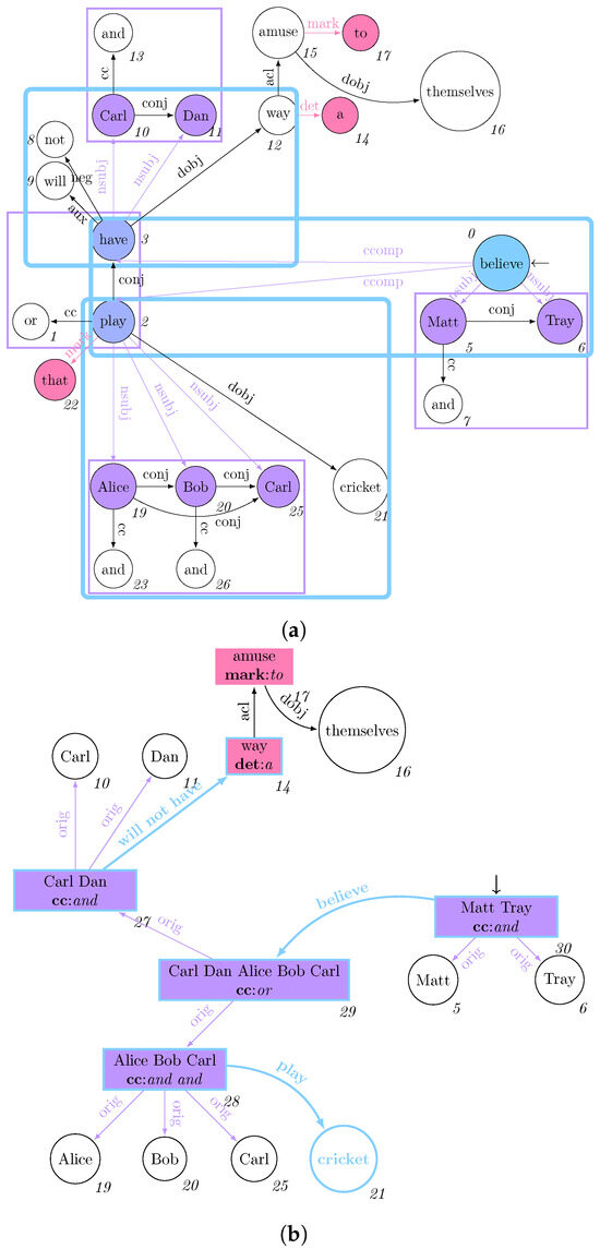
The user is free to break this declarative assumption by directly specifying the order of combination when it is required to combine the values from different variables. This can be observed in a longer query considering more morphosyntactic language features, which is provided online (https://github.com/datagram-db/datagram-db/blob/v2.0/data/test/einstein/einstein_query.txt, accessed on 18 July 2024). This can be used to fully rewrite the database as per Figure 6. As the creation of the will-not-have containment in this will require combining values from vertices 3, 8, and 9 and, respectively, associated with variables V,A, and N, we can use a scripting language as a direct extension of Script v2.0 [34] for determining the order of strings’ composition. Please observe that this formulation, contrary to Neo4j’s APOC in v5.20, also supports optional object matches, where the values associated with non-existingNULLobjects are resolved into empty strings (see Proof for Lemma 7 in Appendix B.3).
Figure 6.
Applying the rewriting rules expressed in Figure 2: different colours refer to different graph grammar rules (b and c), filled vertices in the left (and right) graph refer to the distinct vertex entry-points (and newly generated components). (a) Dependency graph for “Matt and Tray believe that either Alice and Bob and Carl play cricket or Carl and Dan will not have a way to amuse themselves”. While object IDs are presented as numbers, containment IDs are omitted. (b) Generating a binary relationship between the subject as a single entity and the direct object.
By explicitly expressing a containment relationship across the nested entry-point X via so-called hook containments defining equivalence classes, we split the nested morphism into as many new morphisms as the equivalence classes in (see Section 6.3).
Example 5.
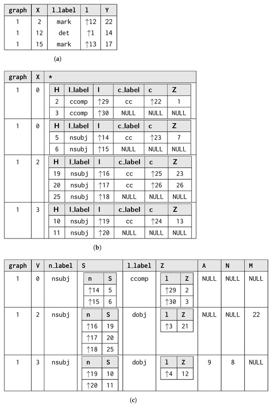
We appreciate the usefulness of such morphism splitting while looking at a more convoluted example, as the one considering the rewriting in the sentence depicted in Figure 6a: vertices Matt and Trayand play and havefrom conjunctions but at different branches of the sentence structure. Furthermore, all four constituent vertices have the same containing vertex believe for which, if no hook relationship was considered, they would have been added within the same morphism as per the previous example.
Still, given that those vertices are associated with different conjas they appear in different coordinating conjunctions, we can use this as a hook relationship to distinguish those, for then obtaining two separate morphisms as illustrated by the first two rows in Figure 7b. Thus, hooks help in splitting nested entry-points structurally by identifying similar elements through structural information.
Figure 7.
Resulting morphisms from the application of the graph grammar rules from Listing 1 over the GSM database in Figure 6a, from which the resulting rewritten database Figure 6b is then obtained. (a) Morphisms . (b) Morphisms , where * refers to sub-matches nested over the entry point (See Algorithm from Section 6.4). (c) Morphisms .
Last, these examples provide an intuitive motivation for why the matching within our query language can express distances of at most one containment relationship from the entry-point match. We want to guarantee that, given two objects matching the query entry-points, located at different distances from the vertex appearing last within the reverse topological order, these are still reachable within the distance of crossing a single containment. Similarly to semistructured data literature, we refer to one as its (direct) ancestor and to the other as its (direct) descendant. If the entry point considering in its match the aforementioned direct descendant object is replaced with another object, be it recently created during the application of the rewriting rules or already existing within the database, we want this information to be passed directly during the execution of the rewriting associated with the match of the object of the direct descendant. For this, we need both an explicit return mechanism, which allows the possibility of explicitly telling the objects appearing at the higher layers induced by the topological order that the previous object has been replaced, and to keep the match size compact, so that we can guarantee that any entry-point value updated at a lower level is retrieved immediately.
6.2. Determining the Order of Application of the Rules
We determine the application order of our language rules for each entry-point vertex of interest (Algorithm 5). This boils down to solving a scheduling problem, which requires first determining the interdependencies across the graph grammar rules. All the matching constructs for each rule in our query gg have variables that might be shared across morphisms.
| Algorithm 5 Sorting the Graph Grammar rules by application order |
|
As per Example 1, each rewriting might replace the entry-points with a single new object, or we preserve the previously matched ones otherwise. These are then input to any later morphism being considered while applying the rewritings. For this, we might consider the variables across patterns as hints to the query language on how the updated or matched objects are going to influence their updates, thus declaring their interdependencies. By reducing this to a dependency ordering, we consider the dependency graphs for the matching and rewriting rules, (Line 4), where each vertex represents a rule (Line 2). Each edge connecting two vertices (or patterns) represents a connection between the entry-point or returned variable from the source pattern and any other non-entrypoint variable occurring in the target pattern (Line 3). As the resulting graph might contain loops as some patterns might exhibit mutual dependencies, we are then forced to run an approximated topological sorting algorithm (Line 5) to determine an approximated scheduling order across such tasks through a DFS visit of the graph [52]: we start traversing the graph from the first rule appearing in the graph grammar while avoiding visiting edges leading to already-visited vertices; if we visited all the vertices reachable from such initial vertex while still having unvisited ones, we recommence the same visit starting from the earliest vertex that was not already visited. We add each visited vertex inside a stack after each of its children has been fully visited. By doing so, we prioritise the rules’ declaration order which then acts as a heuristic for guiding the algorithm to decide upon a specific visiting order.
6.3. Containment Matching
With Algorithm 6, we define the steps realising containment matching for each from a rule to later on generate a morphism table per GSM database , as discussed in Section 6.4. The algorithm works as follows: (i) after caching the PhiTableκ referenced by the containments in the matching patterns to minimize the tables’ access in a uniform schema specification, (ii) we specialise such tables to the specific schema induced by the variables’ names and nesting occurring in the matching . Last, (iii) we collect the matching containments by separating them between required or optional ones.
| Algorithm 6 Intermediate Edge Result Caching |
|
6.3.1. Pseudocode Notation for
We describe the notation used in our pseudocode being the machine readable representation of the query syntax discussed in Section 6.1.
We define each object variable as a pair , where x is the variable name and agg denotes whether the vertex should be aggregated (1) or not (0). In our pseudocode, each matching is represented as the tuple , where specifies the pattern entry-point and each ingoing (or outgoing) edge is represented by a pair , where remarks the variable associated with the container (or contained) object alongside the containment relationship through and , provides a potentially empty-set of containment relationships, is an optional containment variable, all determines whether the edges should be considered in the aggregation or not, and opt determines whether the match should be considered as optional or not. The join edges extend such records as by specifying both the containment () and container () variable explicitly, and hook determines whether the aggregated entry-points over the single incoming container should be subdivided in equivalence classes according to the containment labels in hook, and we perform no clustering otherwise.
6.3.2. Procedural Semantics for Matching and Caching Containments
We now narrate the operations required to match each containment occurring across patterns while representing those as relational tables expressing either required (reqi), optional (opti), or hook-driven equivalence relationships (hooki) per pattern .
First, we define the semantics associated with the matching of each object ego-net as described in ToTable from Algorithm 6 (Line 15): either containment (src)- -[]->(dst) or (dst)<-[]- -(src) are represented as records with fixed schema (Line 9) where each record refers to a single containment (edge) in for a container src, where and dst refers to the contained object; in this, we also retain the containing db as dbid and the containment (edgeLabel). At this stage, all containments are associated with the same schema and are not specialised to abide by a specific schema induced by a matching specification. This allows us to easily cache PhiTableκ containments (Line 30).
Next, we discuss how we specialise the results from the cache according to the schema induced by the variables occurring in each matching . This is carried out by renaming generic containing/containment/contained object labels (src/edge/dst) with the variable names in associated with them; if the patterns also contain references to the edge variable (), we also retain each ID in as , and ’s label (Line 17) and we discard such information otherwise (Line 16). If the edge expresses an aggregation from the container to the content (e.g., (src)–[]–(≫ dst)), we nest (if available) and dst from the table obtained at the previous step (Line 18). This makes the major difference with existing graph query languages, as we consider containment identifiers as a separate class from object ones (thus differently from SPARQL) and we also produce nested morphisms according to the query annotations.
Last, we collect the tables while differentiating where those are associated with a required or optional pattern (Lines 35, 39, and 43), acting as the basic building step for defining nested morphisms as in the subsequent section.
6.3.3. Algorithmic Choices for Optimisation
After discussing the procedural semantics of the matching of containments occurring across all -s, we describe the algorithmic choices for optimisation purposes. First, to minimize the access to a relational database, we ensure that each is accessed at most once across all the edges by collecting all the labels of interest across table-matched containments in queryCache (Line 5). If some containments have no containment attribute specified, we remember the existence of such containment (Line 3) for which we will then require considering all the records, as a containment for which no label is specified forces to consider all the containments (Line 29). Only after this, we access the physical model to transform each PhiTableκ per queryCache to a containment table to be then composed into the final nested morphism table, thus ensuring minimal memory access (Line 30).
6.4. Morphism Instantiation and Indexing
Algorithm 7 combines each table produced from the previous phase to generate the morphisms describing the result of matching through the generation of morphisms being recorded within an table for each GSM database . Similarly to SPARQL’s triple navigation semantics, we generate the morphisms for all GSM databases by natural joining all the tables associated with the mandatory containments (Line 10), while left-joining (the resulting table from the natural join of the required containments) against the optional patterns set and updating with such a result (Line 13).
| Algorithm 7 Morphism instantiation and indexing |
|
We further nest the morphism if and only if the entry-point is aggregated via a single containment object obj (Line 14), for which we then nest in a fresh attribute ⋆ all the attributes except the database where obj is contained, obj itself, and optionally the edge labels for the containment if the pattern exhibits its variable (Line 16).
Hooks derive an equivalence relationship per GSM database having a ⋆-nested morphism through which to optionally split the morphisms. We retain only the container and containment relationship and their containing database ID (Line 32 from Algorithm 6), for then obtaining a suitable equivalence relationship by computing the reflextive, symmetric, and transitive closure of that relationship (Line 17). Then, we potentially split the table nested in ⋆according to the equivalence classes associated with each equivalence relationship obtained from hooks (Line 19) and update the morphism table accordingly.
Concerning the composition of cached tables, to reduce the equi-join time we first sort the tables by increasing size (Line 6) for then stopping the joins as soon as we find or compute an empty morphism, thus entailing that no collection of objects across all dbs can match (Lines 5 and 9). As a last optimisation, we populate collecting the morphisms by database ID and rule ID (Lines 20 and 23). Last, we sort each morphism in by entry-point (Line 4) reverse topological order (Line 26) or, if these were nested in ⋆, by their container object (Line 15). This induces a primary block indexing mapping each elected vertex to a set of morphisms containing it.
6.5. Graph Rewriting Operations (op from )
Finally, we apply the transformation operations required by the rewriting side of the rule for each instantiated morphism in across all GSM databases. This works by keeping track of the desired changes within a GSM view per loaded GSM database.
We now discuss Algorithm 8. For updating GSM views, we apply the rewriting query for each database as described by the rewriting patterns in gg (Line 2): we visit per GSM database its objects according to the reverse topological order from (Line 4) while retaining the objects v appearing in the aforementioned primary block index of a non-empty morphism table for each production rule (Line 5): we skip the morphisms associated with v if either a previously matched vertex was deleted and not replaced with a new one (Line 6), or if the current morphism does not satisfy a possible WHERE condition associated with (Line 8). For the remaining morphisms, we run the operations listed in in order of appearance (Line 9).
| Algorithm 8 Rewriting phase |
|
We now discuss the definition of through SOS semantics enclosed within the evaluation of Line 9 in detail. Figure 8 describes the interpretation of all rewriting rules updating the GSM view , where the first three updates and exploit the functions from Section 4.3. All the y-s are interpreted as evaluated expressions without intermediate assignments. Rule NewObject creates a new object and refers it to the variable j. Rule DelObject deletes a pre-existing or a newly-created object, and Rule DelObject deletes a single container-containment relationship that was defined at loading time. We can easily distinguish between variables referring to objects or containments by the simple type associated with the attribute. For now, we do not allow the explicit removal of containments at run-time unless the containment is explicitly specified via containment update.
We discuss the set update for the vertices’ label values; we distinguish the following cases: if both the number of variable and values are in the same number, we assign for each i-th variable the u-th occurring resolved value (labelZip); otherwise, we assign to each object associated with the resolved variable the collapsed string values (LabelValFlat). We can obtain similar rules for which are omitted here for conciseness, but that can be retrieved in the appendix (Figure A4).


Figure 8.
Graph Rewriting SOS for view update.
Figure 8.
Graph Rewriting SOS for view update.


We treat the property and the containment updates differently, as they deal with the resolution of three variables. We are also interested in whether different resolved variables belong to the same nested table within the morphism or not, with the rationale being that we can freely associate each value within the same nesting row-by-row (P2Zip, P2’Zip, and P2″Zip), while we need to compute the cross-product between the assignments if the value belongs to distinct nestings (Clearly in P3Zip). This is determined via the second parameter of expression evaluation (Appendix A.3) by transferring the attribute information originated by the variable resolution (Appendix A.1). In all the remaining occasions, we arbitrarily decide to flatten the associated expressions. Please observe that, if the querying user wants more control over the precise value to be associated, they can always refer to SCRIPT expressions, thus breaking the declarative assumptions for a more controlled output.
Even in this case, we can formulate the rules for setting the -s similarly to our previous discussion for the -s. Therefore, we defer to Figure A5 provided in the Appendix A.4.
We conclude by analysing the semantics associated with the replacement via ’s return statement, the last and mandatory operation for declared rewriting operations. We apply no rewriting if the returned variable is the variable entry-point (NoRewr). Otherwise, if the entry-point variable is not aggregated, we resolve the replacement and entry-point (Repl and Orig, respectively) and we replace any object in Orig associated with the entry-point variable with an object in Repl associated with the replacing variable (NoAggrRewr). Otherwise (AggrRewr), the rewriting occurs by replacing the objects in Orig, associated with the entry-point’s container and the objects in Repl, associated with the returned variable p′. Furthermore, given C the containment labels for which the entry-point is contained by its aggregating object in cont, we also update the containing for the cont objects to also contain via C the replacing objects in Repl. As this provides the final update, we then consider this last resulting GSM view of the resulting view for our rewriting step.
As no SOS rule matches the empty string, no further operation is conducted, and the rewriting program terminates after considering the final rewriting statement.
7. Language Properties
Given the previous language description, we want to characterise its properties by juxtaposing them with Cypher’s. Full proofs are provided in Appendix B.3. We start by showing that, unlike current graph query languages, we propose a rewriting language framed as generalised graph grammars: we relate our proposed language to the graph grammars as, similarly to these, the absence of a matched pattern leads to no view updates. Still, we claim that such language provides a generalisation of the former by supporting explicit data-aware update operations over the objects and containments, while also defining explicit semantics determining the order of the application of such rules, both across rules and within each GSM database.
Lemma 6.
If either we query all the GSM databases with no rules, or all the rules have no rewritings, or none of the matches returned a morphism, or none of the ones being matched pass the associated Θ condition, then we return the same GSM databases as the ones being originally loaded.
Next, we ensure that the rules are applied in reverse topological order, thus minimising the restructuring cost of the GSM database while achieving declarativeness for rule application, as the user does not specify this within the query formulation, as no matched pattern leads to no view updates.
Property 1.
The rules are applied in (reversed) topological order while visiting each GSM.
On the other hand, we can show that Cypher forces the user to specify in which order the updates shall be applied, thus breaking the declarative assumption for a good query language.
Lemma 7.
The application of the rewriting in Cypher in lexicographical order requires explicitly determining the order of the morphisms’ application and the order of the graph’s visit.
Next, we state the usefulness of an explicit return statement within the interpretation of a rule as it allows us to propagate the updates on the subsequently evaluated morphisms.
Lemma 8.
If an entry-point match is deleted and a new object is re-created inheriting all of its properties, this new object will not be connected to the entry point’s containers unless the newly-returned object was applied.
To a minor extent, we also show a greater amount of declarativeness if compared to current graph query languages by automatically generating a new object if an update operation occurs with reference to an optionally matched variable that was not matched to an existing object.
Lemma 9.
The setting of properties to variables not associated with a newly-created object variable and not associated with an actual GSM object due to an optional match reduces to the creation of a new object associated with the variable, which then always receives this and any following update associated with the same variable.
At this point, it could be argued that, although our proposed rewriting language performs queries that cannot be expressed in other graph query languages, this does not return the matched subgraphs as in such other languages, similar to Cypher’s return statement due to the considerations from Lemma 6. The following Lemma shows otherwise. Thanks to this, this language is considered more expressive than Cypher.
Lemma 10.
The proposed graph grammar query language can express traversal queries retaining only the objects and containments being matched and traversed.
Corollary 1.
The proposed graph query language is more expressive than current graph query languages.
8. Time Complexity
We now study the computational complexity associated with the algorithms discussed in the previous section and infer this from the implementation details discussed while reasoning on the SOS discussion. Proofs are postponed to Appendix B.4. Please observe that, as previously noted from previous graph query language literature (Section 3.1.2), the following results do not intend to prove P vs NP, as we are deliberately expressing a sub-problem of the more generic subgraph isomorphism problem that can be easily captured through algebraic operations.
Lemma 11.
The time complexity of sorting the rules within the query is quadratic over the number of query rules.
Lemma 12.
The intermediate edge result caching time complexity has a polynomial cost being linear in both the loaded databases and the number of available objects.
Corollary 2.
The cost for generating the nested morphisms is polynomial with the size of the entire data loaded within the physical model.
Lemma 13.
The rewriting cost is polynomial and linear with the number of rewriting operations and the number of the morphisms.
Corollary 3.
The time complexity of the whole Generalised Graph Grammars is polynomial with the size of the loaded physical model.
9. Empirical Evaluation
For our empirical evaluation, we study the use case of graph grammar in the context of rewriting graphs representing the grammatical structure of a natural-language sentence. Universal dependencies [53] capture these syntactical features across languages by exploiting a shared annotation scheme. In this context, the usual approach to graph rewriting boils down to rewriting a PROLOG-like logical program by applying declarative rewriting rules (https://github.com/opencog/relex accessed on 22 April 2024) via a unification algorithm [54], where compound terms are equivalently expressing binary relationship and properties associated with specific vertices. Given the general interest for such an approach within the domain of Natural Language Processing (NLP), the present paper is going to specifically focus on use case scenarios within such domain. This will also give us the opportunity to re-use freely available datasets for sentences for our experiments (https://osf.io/btjqw/?view_only=f31eda86e7b04ac886734a26cd2ce43d and https://osf.io/rpu37/, accessed on 21 April 2024), which can be then deemed as repeatable.
Notwithstanding the previous approaches, we want to achieve a more data-driven approach to sentence rewriting, where atoms can also be associated with properties and labels, thus motivating the definition of the proposed query language. Furthermore, the extension of the graph grammar language with a script can be used to compose data and define boolean conditions allowing us to break the declarativeness assumption only when the user wants more control over how data are processed. Thus, we postulate that our proposed query language extends the current literature in several aspects way beyond graph database literature while postulating the possibility of applying concurrently multiple rewriting rules over disparate sentences via a sole declarative query. The proposed approach shares some similarities with programming language research where, after representing a program in terms of its operational semantics, we can apply graph rewriting rules over abstract semantic graphs [55], which are usually represented as trees, for which similar considerations like the former can be applied.
We test the implementation of our physical model and associated query language as implemented in our novel object-oriented database, named DatagramDB, which source code associated with the current paper is freely available online (https://github.com/datagram-db/datagram-db/releases/tag/v2.0, accessed on the 22 April 2024). We conducted all our benchmarks on a Dell Precision mobile workstation 5760 running Ubuntu 22.04 LTS. The specifications of the machine include an Intel® Xeon(R) W-11955M CPU @ 2.60 GHz x16, 64 GB DDR4 3200 MHz RAM.
9.1. Comparing Cypher and Neo4j with Our Proposed Implementation
Given the problems being evidenced by the Cypher query language from Lemma 7, we cannot automate the benchmarking of Cypher for all the possible sentences coming from an online available dataset. By recalling the results of this lemma, we observe that, when the query is not able to capture a pattern albeit optionally, this will have a cascade effect on the entire query for which none of the following rewriting operations will be applied. Given this, the same query might not necessarily provide the same output across different sentences having a different sentence structure. Thus, we cannot use one single query for dealing with unpredictable sentence structure that, in the worst-case scenario, would require us to write one single query per input sentence. We then preferred to limit our comparison to two sentences, for which we designed the minimal Cypher query exactly capturing the syntactical features expressed by these sentences while using the same query for DatagramDB across all the sentences.
We considered two distinct dependency graphs: “Alice and Bob play cricket”, the one in Figure 3a, and the one resulting from the dependency parsing of the “Matt and Tray...” sentence from Figure 6a. We loaded them in both Neo4j v5.20 and our proposed GSM database. In Cypher, we then run the query as formulated in the previous section, while we construct a fully declarative query in our proposed graph query language syntax directly representing an extension of the patterns in Figure 2. From now on, when referring to Neo4j, we will always refer to version 5.20.
Examining Table 1, we can see our solution consistently outperforms the Neo4j solution by two orders of magnitude. Furthermore, the data materialisation phase does not significantly impact the overall running time, as its running times are always negligible compared to the other ones. Additionally, Neo4j does not consider a materialisation phase, as the graph resulting from the graph rewriting pattern is immediately returned and stored as a distinct connected component of the previously loaded graph. This then clearly remarks the benefit of the proposed approach for rewriting complex sentences into a more compact machine representation of the dependency graphs.

Table 1.
Table displaying results from rewriting the aforementioned sentences.
9.2. Scalability for the Proposed Implementation
For testing the scalability of our implemented system, we used a corpora of sentences used for natural-language common-sense question answering [56] which we rewrote into dependency graphs using Stanford NLP [57]. As its output is failing systematically at correctly recognising verbs in passive form when at the present time and at recognising negations due to its training-based nature [58], we provide a piece of software amending its output so that all the syntactic and the semantic information retained within the sentence could pertain in a graph structure. This server also transforms the internal Stanford NLP dependency graph into a collection of GSM databases serialised in textual format. The resulting server is available online (https://github.com/datagram-db/stanfordnlp_dg_server accessed on 19 April 2024).
Given the resulting GSM representation of the two sentences, we provide two distinct scalability tests: in the first one, we sample the dataset into sentences to determine the algorithm’s scalability in terms of both the number of GSM databases and the number of vertices, while in the second we will only consider scalability regarding the sole number of GSM databases while maintaining the sample distribution of the sentence’s lengths, thus reflecting the number of GSM objects within the database.
Concerning the first scenario, we choose the sentences containing words, and for each of them we choose 300 sentences each, thus obtaining sample sets . Then, we further sample into three distinct subsets having cardinality of for which for and . This will be useful to then plot the rewriting running times using for the x-axis either the number of sentences (or GSM databases) or the sequence length, to better analyze the overall time complexity. The results for these experiments are reported in Figure 9.
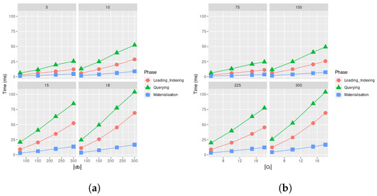
Figure 9.
Analysing DatagramDB. (a) Results grouped by number of words per sentence. (b) Results grouped by number of databases.
From these plots, we can clearly remark that querying and materialisation times are clearly linear over the size of objects being loaded or GSM databases being matched and rewritten, thus remarking the efficiency for the overall envisioned approach: please observe that we cannot achieve a better time complexity that a linear scan without additional heuristics, as we still have to perform the visit over each GSM database by also performing a linear scan of the database objects in reverse topological (layered) order. We can also motivate these results by having graphs in which the branching factor is relatively small compared to the overall number of available vertices, thus for each GSM database . We also observe that, for these smaller datasets, the resulting materialisation time is almost negligible compared to the query time, which, across the board, dominates the loading and indexing time.
By comparing such running times with the ones from Neo4j, we can easily observe that, while we were able to process 300 GSM databases in 100 milliseconds, Neo4j could rewrite just one single graph in double time. Given this, our approach has a throughput of almost 600 times over Neo4j. This further remarks the impracticality of using the competing solution for analysing more sentences in the future, e.g., while considering sentences crawled from the web.
While it might initially seem that all phases (loading, querying, and materialisation) exhibit linear time complexity, we will try to consider a larger set of data to better outline the time complexity associated with our implementation.
Concerning the second scenario, we decided to sample the internet dataset in a subset of sentences where . S represents the entire dataset while ensuring that each dataset of a lesser size is always contained in the larger dataset. Furthermore, we ensure that the number of words, and therefore, of objects on each sampled database reflects a similar frequency distribution of the number of objects per resulting GSM database (Figure 10). By doing so, for our final scalability tests in which we consider more data, we make up for the lack of long sentences with the number of sentences reflected in the number of the GSM databases to be processed.
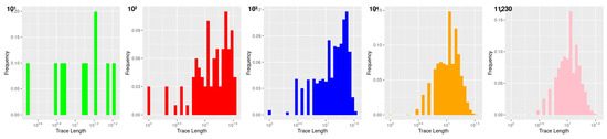
Figure 10.
Sampled probability density function associated with the number of words within the sentences for each subset of traces.
Figure 11 provides the benchmarks for these experiments: a non-linear but polynomial loading time might be possibly related to the data parsing time and the time to store such data in primary memory, while the remaining running times keep a linear time complexity concerning the increase in the number of the GSM databases to be rewritten, similarly to the previous experiments. Querying time always dominates in indexing time by at least one order of magnitude, thus showing that most of the significant computations occur while matching and rewriting. Materialisation times are on the same order of magnitude as indexing time, thus also showing that this cost does not exceed the actual querying phase. Overall, the efficiency of our system is also reflected by a linear querying time for the datasets being considered.
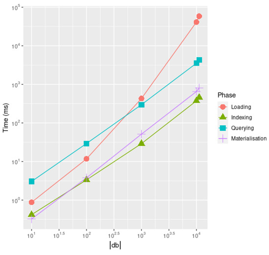
Figure 11.
Running time of each algorithm with different sentence samples.
10. Conclusions and Future Works
This paper offers the definition of a matching and rewriting mechanism similar to the one provided by graph grammar implemented over object-oriented databases. As our definition supports both data matches and complex data update operations over the objects of interest, whose features were not considered in previous graph grammar formulations, we name our proposed language Generalised Graph Grammars. Our theoretical results prove the impossibility of expressing the same query with the same degree of generality of Cypher, which requires specifying a different query for any potential graph to be queried, thus posing a major limitation to automating rewriting operations over graphs. Empirical results prove that our query language offers an implementation faster than the ad-hoc query formalised in Cypher and run over Neo4j v5.20, in terms of both running time and throughput expressed in the number of queries runnable per comparable amount of time. These results aim to observe the inadequacy of graph-centric implementations of data representations since a large amount of literature now agrees in stating that more traditional and relational representations often offer better performances with respect to queries both natively supported by graph languages [59] and in representing new operations on graphs that require their rewriting [6,7].
At this stage, we considered nested morphisms of at most depth of 1, thus requiring that each cell of a morphism table should contain at most one non-nested table. Future works will investigate whether there might be any benefit for further generalising this nesting to arbitrary depth, thus requiring further extending the definition of the Nested Natural Equi-Join operator to arbitrary depths.
Notwithstanding the possibility of the current model expressing uncertainty within the data, the rewriting operations always assume to deal with perfect information, thus generating objects or containments containing no uncertainty. Future works will address this gap by further extending the SOS semantics of these rewriting steps while considering provenance information [44], thus relieving the user from explicitly defining the uncertainty of the generated data by adding further declarativeness to the query language here proposed.
Although Lemma 10 showed that the proposed graph query language is also able to remove the unmatched objects and contents, our current algorithm is not tailored for effectively matching this case, as the removing pattern will be forced to return all the objects and containments for then removing them. Future works will extend this by optimising testing conditions for our general language while matching the objects and containments. As a direct consequence of this, our returned morphisms are not pruned after testing the condition, which is just evaluated in the rewriting phase due to the fact that any updates to the GSM views will also alter the outcome of . Future works will use static analysis approaches to determine when can be effectively used for pruning morphisms before being returned in the matching phase, and condition rewriting strategies to push condition evaluations towards the generation of the morphism as discussed in Section 6.3 and Section 6.4.
Although the current language supports the update of objects and containments within GSM objects, the provided query semantics do not consider the possibility that such updates can be still matched by the query, thus triggering additional rewriting operations. Future works will also consider further generalising the database matching and rewriting approach by considering the fix-point over the loaded database until convergence is met, thus meeting the former desiderata. We will also consider extending our containments with property-values associations similarly to the property graph model, and considering updating the objects’ and containments’ costs while performing the rewriting operations.
Last, preliminary experiments [34] conducted on a physical model being the direct mapping of the logical model in memory provide promising results showcasing the possibility of expressing not only JSON files but also representing indexing data structures in GSM that eventually lead to scalable query processing for JSON data. Future works will also compare the efficiency of DatagramDB if compared to other databases supporting object-oriented representations such as MongoDB or MySQL [60].
Author Contributions
Conceptualisation, G.B. and O.R.F.; methodology, G.B.; software, G.B. and O.R.F.; validation, G.B. and O.R.F.; formal analysis, G.B.; investigation, O.R.F.; resources, G.B.; data curation, O.R.F.; writing—original draft preparation, G.B.; writing—review and editing, O.R.F. and G.M.; visualisation, G.B. and O.R.F.; supervision, G.B. and G.M.; project administration, G.B.; funding acquisition, G.B. All authors have read and agreed to the published version of the manuscript.
Funding
This research received no external funding.
Data Availability Statement
The datasets are available at the following repositories: https://osf.io/btjqw/?view_only=f31eda86e7b04ac886734a26cd2ce43d and https://osf.io/rpu37/. The codebase associated with the implementation of the data model and query language interpretation are available on GitHub: https://github.com/datagram-db/datagram-db/releases/tag/v2.0. All the URLs were accessed on the 21 April 2024.
Conflicts of Interest
The authors declare no conflicts of interest.
Abbreviations
| BNF | Backus-Naur Form |
| DAG | Direct Acyclic Graph |
| GSM | Generalised Semistructured Model |
| HOF | Higher-Order Function |
| NLP | Natural Language Processing |
| SOS | Structured Operational Semantics |
Appendix A. Full Definitions
Appendix A.1. Variable Resolution
Before discussing value or boolean expression evaluation, we need to consider their base case first, which is the evaluation of variables occurring in such expressions. We, therefore, discuss these first before introducing the other steps. We consider variables referring to both objects and containments while supporting the update operations only for the latter. We, therefore, resolve the variables while returning the IDs for either matched objects or containments.
We, furthermore, want to achieve declarativeness while considering variables: if associated with NULL values as a result of a missed optimal match, we want to return empty values, while if we set values to them, we want to create implicitly new vertices. We need to then provide a new parameter to explicitly consider the creation of new objects when the expression context allows us to do so over unreferenced and unmatched variables. Furthermore, the single variable might be associated with multiple objects if referring to a morphism attribute within a nested relationship. Since the resolution of variables within our language may require to access previously replaced or substituted values such as from , we also have to refer to and g to carry out the variable resolution.
Since these operations can also involve updating the environment, we express these operations via SOS rather than using algebraic notation. Figure A1 shows the SOS for the sole variable resolution, returning a tuple containing (in order of appearance) the resolved variables, the possibly updated view due to object insertion, and the potentially nested attribute containing a nested table expressing the variable as an attribute.
If the variable belongs to the morphism’s schema and is associated with a non NULL value within the morphism while being associated with a basic type, we return the value stored in it (ExRes). If the variable refers to a nested attribute, we resolve the variable (, Equation (11)) and return all the associated values via (Definition 6, ExResNest). If the variable was declared within the rewriting pattern alongside the creation of a new object, we return the ID associated with the newly created object (NewRes). If the variable is neither newly declared nor in the morphism’s schema, we return no result, as there os no binding and the query language is not expected to return a value (NoRes). Last, if we require the object to be created (new=true) as we set values associated with an object and the morphism did not return an object ID associated with x due to an optional match, we then create a new object in the GSM view associated with a fresh value, while returning the updated view (ForceRes). This behaviour is completely disabled and no view is updated if the original expression does not force the creation of a new object due to an expression evaluation (NoFRes). In all the other circumstances, we resolve no reference IDs (NoFCRes).

Figure A1.
Variable resolution with potential view updates ().
Figure A1.
Variable resolution with potential view updates ().

Appendix A.2. Predicate Evaluation (Θ)
We now discuss boolean predicate evaluation: given that the variables might refer to nested attributes referring to multiple objects or containment, for which we are interested in comparing the labels, values, or properties associated with them, we might be interested in returning not only one single boolean value but one single boolean value per comparison outcome. Given this, we need a notion of sets explicitly remarking that some elements were not inserted. A maximum cardinality set is a pair of a set S and a natural number n denoted as such that . This type of set can be used to efficiently represent how many elements satisfy a given condition if the number of elements is previously known. So, if , we know that not all the n elements of interest satisfy a given condition. We also constrain such sets to contain at most n items. We can easily override traditional set operations over such sets as follows
We say a maximum cardinality set is full if the cardinality of S is equal to n: . We say that such maximum cardinality set is empty if S is empty: . The cardinality of the maximum cardinality set is the cardinality of its constituent set: .
Figure A2 provides the definition providing the considered semantics. For this, we require that two original variables refer to the same cardinality of values, or that at least one of them is associated with one single value (TestComp). For this, we can then return a maximal cardinality set where S indicates the resulting tuple indices associated with a true value, and M refers to the maximum size of the morphisms.

Figure A2.
Predicate Evaluation semantics .
Figure A2.
Predicate Evaluation semantics .

Furthermore, we might also be interested in determining whether objects being matched in the current morphism also appear (TestMatch) or not (TestUmatch) in another morphism L associated with a variable y. Given that we are interested in the objects actually being matched and not in later changes provided by subsequent transformations, we can simply refer to listing the reference IDs associated with an attribute X in . This can be easily represented as a maximum cardinality set by stripping the NULL values, while returning the intersection (TestMatch) or the difference (TestUmatch) for those IDs.
As the tests in the second last paragraph will return no sets whose indices are released to neither object nor containment ID while the former will return such indices, we need an intermediate predicate where these two set-boolean results are computed, to return for the former a full maximum cardinality set containing all the ID references from the morphism if the underlying expression will not return an empty maximum cardinality set (TestFill).
We associate a similar behaviour to the typecasting of a script evaluation to a boolean value, for which we return an empty set if this is false and tall the occurring references within the morphism otherwise (TestScript).
Last, we interpret the conjunction and the disjunction of such multivalued boolean semantics as the intersection (TestConj) or the union (TestDisj) at the set of reference ID satisfying the base case candidates.
Appendix A.3. Expression Evaluation (expr)
Last, we are interested in evaluating expressions exploiting the variables withheld by each morphism. Please also observe that these expressions will have different operational semantics if compared to the ones associated with assignments, as the former will only retrieve values associated with the expressions, and the latter describe how to update the view with the newly assigned value. For this, these expressions will only return the final value associated with them. As the morphisms might be also nested, their final representation will be a one-column table with an arbitrary attribute, for which time is one of the basic types.
Figure A3 shows the SOS associated with the expression evaluation. From this, we provide as a shorthand for the above relationship:
In other words, computes the first projection of , being the evaluation of an expression x.


Figure A3.
Expression evaluation (E) with no view update, where is an expression returning y if x holds and z otherwise.
Figure A3.
Expression evaluation (E) with no view update, where is an expression returning y if x holds and z otherwise.


For the evaluation of the attribute associated with a containment ID (LabelE), we directly apply to all the non-NULL matches, as containment IDs are never updated in this version of the language. For extracting values (XiE) or labels (EllE) associated with the object x at the numerical index idx not associated with an evaluated expression, we resort instead to the Property Resolution function also encompassing the changes in the GSM view (Definition 6). The interpretation of considers both x and str as expressions, where only the former is forced to be interpreted as a variable if is a string: if x and str are associated with a tuple of values V and P of the same cardinality, we then return for (ContZipE), and if otherwise we return for (ContE).
Last, for conditional expressions, we first evaluate a condition which, as per the forthcoming discussion, will return a set of object or containment IDs for which the entire expression holds. If such a set is full, we return the evaluation of the expression associated with the “then” branch (AllTrueE), if it is empty, we return the evaluation of the expression associated with the “else” branch (AllFalseE), and otherwise, we first interpret over the IDs referenced by a variable x, and then return the i-th value from the left expression if the MES associated with contains the i-th object reference after x, and the i-th value from the else branch otherwise.
If we need to evaluate the string as a variable as it appears as the leftmost argument of a label, , ℓ, or , then we use variable resolution (Appendix A.1 on page 42) to evaluate the values associated with the variable (VarE), and we consider this as a simple string otherwise (StrE). Please observe that this invented value is then associated with an unexisting nested morphism .
Appendix A.4. Full SOS Rewriting Specifications
This section describes through Figure A4 and Figure A5 the remaining set-update operations that were not reported in Figure 8 for conciseness. These refer to updates (Figure A5), similar to the ones for ℓ, and (Figure A5), similar to the ones for .

Figure A4.
Remaining setting functions for -s being the extension of Figure 8.
Figure A4.
Remaining setting functions for -s being the extension of Figure 8.


Figure A5.
Remaining setting functions for -s being the extension of Figure 8.
Figure A5.
Remaining setting functions for -s being the extension of Figure 8.

Appendix A.5. Converting GSM from Any Data Representation
Listing A1. 


Python code showing the conversion of an arbitrary Python object representation of some data to a GSM representation. In particular, we showcase the conversion of (possibly nested) Pandas dataframes, XML data, NetworkX graphs, and XML trees. As we also showcase the representation of arbitrary Python objects, thus including linear collections and dictionaries, we also support JSON conversion.
Appendix B. Proofs
Appendix B.1. Transformation Isomorphism
Proof (for Lemma 1).
Proving this reduces to prove that and . We can prove this by extending the definition of the transformations being given in Algorithm 2.
- : We can consider one GSM database being returned at a time, for which we consider its constituents . To do this, we want to show that such a returned database is equivalent to the originally loaded . To conduct this, we need to show that each of the constituents is equivalent.We can prove that as follows:We can prove that , , and as follows:We can also prove that the properties are preserved:For , we can easily show that this is associated with no value only if there are no records referring to a containment for j in the loaded database, which we can easily show that this derives from an originally empty contained from the loaded database . On the other hand, this function returns a set S of identifiers only if there exists at least one containment record in PhiTableκ, for which we can derive the following:Given that and , this sub-goal is closed by transitivity closure over the equality predicate.We can prove similarly the equivalence as a corollary of the previous sub-cases:
- : In this case, we need to show that each table in is equivalent to those in . We can prove similarly to the previous step that , , and .Next, we need to prove that the ActivityTables being returned are equivalent. We can achieve this by guaranteeing that both tables should contain the same records. After remembering that the values of p and x are determined through the indexing phase, from which we determine the offset where the objects with immediately preceding and following IDs are stored, we can then guarantee that these values will be always the same under the condition that the two tables will always contain the same records, for which these values will be the same. After remembering from the previous proof that , for and , we can also have that :Given that the first three components of the record always correspond, this entails that we will preserve the number of records across the board, hence preserving the same record ordering, thus also guaranteeing that and .By adopting the equivalence of the previous and next offset for the AttributeTable from the previous sub-proof, we can then also prove that each record of the always corresponds to an equivalent one in the AttributeTable.Given that we can prove that also by the previous sub-case and as the records’ index will always correspond after sorting and indexing, we can close this sub-goal.Last, we need to prove that the tables are equivalent, which can be closed as follows:
□
Appendix B.2. Nested Equi-Join Properties
Proof (for Lemma 2).
If with , then we can rewrite the definition of as follows:
If , then by assuming to represent a NULL value as an empty table by default. While doing so and by by former assumption, the former result can be rewritten as:
□
Proof (for Lemma 3).
Given the hypothesis and with reference to Algorithm 3, we have , which then yields (Line 4). □
Proof (for Lemma 4).
Given the hypothesis and with reference to Algorithm 3, this satisfies the condition at Line 5, for which we can then immediately close our goal. □
Proof (for Lemma 5).
As , this violates the condition for the rewriting Lemma 3, which is not then rewritten accordingly. Furthermore, the condition violates the condition for the rewriting Lemma 4, which is then not applied. Given as defined in Line 3 of Algorithm 3, we show that this algorithm computes the following:
This equates to equi-joining the tables over the records where by construction, and by nesting all the records from the right table sharing the same values with the records from the left table. Last, we can easily observe that this cannot be easily expressed in terms of , as the rewriting of the former expression in the following way, for which it is evident that the former operator did not consider the recursive natural joining of the records by considering the commonly-shared attributes during its descent:
This can be easily observed by the lack of component that captures the essence of such a natural join condition. □
Appendix B.3. Language Properties
Proof (for Lemma 6).
As by the conditions stated in the current Lemma we either generate an empty morphism table (no rules, no rewritings, no matches) or all the generated morphisms are ignored as all the values are falsified (Line 8 from Algorithm 8), then we will always have an empty view for all the GSM databases loaded in the physical model. Considering this, the proof is an application of Equation (10), by which the materialisation of a GSM database with a view containing no changes simply returns . As is stored in a physical model, this result is also validated via Lemma 1. □
Proof (for Property 1).
This condition is generated by Line 4 from Algorithm 8, as we use the reverse topological order index associated with each GSM DB to visit the entry-point objects or, when nested, their containing object associated with the reported morphism in . □
Proof (for Lemma 7). 
As per previous discussions, the proof for this lemma will be given intuitively by analysing the Cypher representation of the graph grammar represented visually in Figure 2 and previously represented by our proposed Generalised Graph Grammar language in Listing 1. We then provide the query required for rewriting the sentence expressed in Figure 6a:
The current Neo4j v5.20 implementation does not support the theorised graph incremental views for Cypher [32]. As we require to update the graph while querying, it is not possible to entirely create a new graph without restructuring or expanding a previously loaded one as per graph joins [7] or nesting [6] by simply returning some newly-created relationships or vertices; returning a new graph and rewriting a previous match will come at the cost of either restructuring the previously loaded graph, thus requiring additional overhead costs for re-indexing and updating the database while querying, or by creating a new distinct connected component within the loaded graph ( statements from Listing A2). As it is impossible to refer by the vertices and edges through their ID, thus exploiting graph provenance techniques for mapping the newly created vertices to the ones from the previously loaded graph [45], we are forced to join the loaded vertices (e.g., Lines 35–37, 50–52, and 67) with the newly created ones (e.g., Lines 38, 53, and 68, respectively) by their property values (e.g., Lines 39, 54, and 70, respectively). Our proposed approach avoids such cost via the aforementioned objects’ and containments’ ID-based morphism representation while keeping track of the restructuring operations (property Update, insertion NewObj, deletion DelObj and DelCont, and substitution ReplObj) over a graph g within an incremental view (Section 4.3).
statements from Listing A2). As it is impossible to refer by the vertices and edges through their ID, thus exploiting graph provenance techniques for mapping the newly created vertices to the ones from the previously loaded graph [45], we are forced to join the loaded vertices (e.g., Lines 35–37, 50–52, and 67) with the newly created ones (e.g., Lines 38, 53, and 68, respectively) by their property values (e.g., Lines 39, 54, and 70, respectively). Our proposed approach avoids such cost via the aforementioned objects’ and containments’ ID-based morphism representation while keeping track of the restructuring operations (property Update, insertion NewObj, deletion DelObj and DelCont, and substitution ReplObj) over a graph g within an incremental view (Section 4.3).


Cypher does not ensure to apply the graph rewriting rules as intended in our scenarios: let us consider the dependency graph generated from the recursive sentence “Matt and Tray believe that either Alice and Bob and Carl play cricket or Carl and Dan will not have a way to amuse themselves” and let us try to express patterns in Figure 2b,c as two distinct  -es with their respective update operations as per the following Listing:
-es with their respective update operations as per the following Listing:Instead of generating one single connected component representing the result, we will generate as many distinct connected components as subgraphs being identified as matching the patterns, while this does not occur with a simple sentence structure (Figure 3a) where we achieve the correct result as in Figure 5. We must elements of the graph multiple times, constantly rejoining on data previously -ed in earlier stages of the query for establishing relationships over previously grouped vertices (Lines 108 and 118 from Listing A2). This then postulates the inability of such language to automatically apply an order of visit for restructuring the loaded graph (e.g., we need to tell the query language to first group-by the vertices—Lines 2–15—and then establish the orig relationships—Lines 18–24) while not expressing an automated way to merge each distinct transformed graph into one cohesive, connected component. This then forces the expression of a generic graph matching and rewriting mechanism to be dependent on the specific recursive structure of the data. Thus, requiring the creation of a broader query, where we need to explicitly instruct the query language on the correct way to visit the data while instructing how to reconcile each generated subgraph from each morphism within one final graph.
elements of the graph multiple times, constantly rejoining on data previously -ed in earlier stages of the query for establishing relationships over previously grouped vertices (Lines 108 and 118 from Listing A2). This then postulates the inability of such language to automatically apply an order of visit for restructuring the loaded graph (e.g., we need to tell the query language to first group-by the vertices—Lines 2–15—and then establish the orig relationships—Lines 18–24) while not expressing an automated way to merge each distinct transformed graph into one cohesive, connected component. This then forces the expression of a generic graph matching and rewriting mechanism to be dependent on the specific recursive structure of the data. Thus, requiring the creation of a broader query, where we need to explicitly instruct the query language on the correct way to visit the data while instructing how to reconcile each generated subgraph from each morphism within one final graph.During the delineation of the final Cypher query succeeding in obtaining the correct rewritten graph (also Listing A2), we also highlighted the impossibility of Cypher propagating the temporary result generated by a rewriting rule and propagating it to another rule to be applied upstream: this requires carrying out intermediate sub-queries establishing connections across patterns sharing intermediate vertices, and the re-computation of the same intermediate solutions, such as vertex grouping (cfr. Line 4 and Line 116). Since Cypher also does not support the explicit grouping of vertices based on a pattern as in [46], this required us to identify the vertices satisfying each specific pattern, label them appropriately in a unique way (e.g. Line 9), and then compare the result obtained (e.g., Line 20 for generating orig relationships). This limitation can be overcome by providing two innovations: first, using nested relational tables for representing morphisms, where each nest will contain the sub-pattern of interest possibly to be grouped. Second, we track any vertex substitution for entry-point vertex matches via incremental views. This substitution can be easily propagated at any level by considering the transitive closure of the substitution function (Definition 5), while the order of visit in the graph guarantees the correctness of the application of such substitution (Algorithm 8).
Listing A2, constructed for the specific matches referring to the sentence “Matt and Tray...”, will not fully execute on a different sentence without the given dependencies, as no match is found, and therefore, no rewriting can occur. Current graph query languages are meant to return a subgraph from the given patterns. In Cypher, you must abide by what is contained within the data, if the data are not there we need to remove the match from the query, which we cannot forecast in advance. This results in constant analysis of the data. For us, the intention is to have graph grammar rewriting rules whereby if a match is not made, no rewriting occurs.
By leveraging such limitations of Cypher while juxtaposing the desired behaviour of the language, we derive a declarative graph query language where patterns can be expressed similarly to Figure 5. □
Proof (for Lemma 8).
This is a direct application of the SOS rules from Figure 8: any removed vertex will not be replaced by a newly inserted vertex within the matched entry-point ego-net if not explicitly updating the containment to also add the newly created object. If an entry-point was removed, the only way to preserve the connectivity of the GSM objects is to exploit the replacement, through which we will explicitly state that, for any explicitly declared container within the matched pattern, we will insert the created object or any other previously matched object of choice within the container’s containment relationships also containing the object. □
Proof (for Lemma 9).
This requires discussing the SOS rules from Figure 8, from which we set or update values, labels, containments, and properties associated with objects. Concerning label updates, such updates occur over variable x, in which variable resolution is always in the form : if the variable does not appear in the morphism, we expand the first two cases from Figure A1. We need to exclude the case it was declared with a new statement from Figure 8, as we will have otherwise x in from . As we have the parameter true, this also excludes the rule NoFRes (Figure A1). We can then see that we do not create an optimally matched containment, as expected by the intended semantics. Thus, we restrict our case to ForceRes (Figure A1), on which we see that a new object is created, thus updating , and that we know the ID of this object as it will be naturally the next incrementally number being available. Then, the label update will always occur, which will then preserve the update in . These choices are reflected in the materialisation phase by extending each database g and prioritising the changes described in the view . □
Proof. 
Given the possibility of visiting several patterns , we can express the matching of those in our proposed query language as rules for , where both objects and containments must be explicitly referenced with a variable. Still, this formulation will not explicitly remove any object or containment not being visited. Enabling this requires the extension of the former query with two additional rules, one for removing all the vertices not visited in the different pattern (om), and the other for explicitly removing unmatched containments (cm). Given the variables referring to matched objects and to matched containments in , we can then express om and cm as the following rules being defined immediately after :
As we rewrite the same matching object, no replacement will occur and given that the matching (Z) and (X)–[Y:]->(Z) will return all the objects and containments across the databases, we have to further test those to delete only the ones being not matched in . □
Proof (for Corollary 1).
This follows from our previous proof, for which we clearly showed that our proposed language can match and rewrite graphs declaratively while considering optional rewrites. Cypher has some limitations in this regard, as it forces the user to specify the order in which the matching and rewriting rules should be applied. Furthermore, our language can return the matched morphisms similarly to SPARQL while allowing the generation of multiple morphism tables rather than just one, and selecting just the objects and containments being matched while removing the remaining ones similarly to Cypher. Therefore, the proposed language over GSM generalizes over current graph query languages over a novel generalised semistructured model enabling this. □
Appendix B.4. Time Complexity
Proof (for Lemma 11).
Regarding Algorithm 5, as we defined a graph connecting each rule appearing in the query, which will be then represented as a vertex, in the worst-case scenario, we will have a fully connected graph with . Thus, the cost of creating this graph is quadratic, as is in . Given that the approximate topological sort uses a DFA visit of the resulting graph and that the layering is linear over the size of the vertices, and given that by construction we, therefore, obtain an overall global quadratic time complexity over the size of the query when expressed via the number of available rules. □
Proof (for Lemma 12).
Suppose that each rule has at most c containment relationships, which will be provided by disjunction reference to all the k containment labels recorded in the physical model. Thus, the caching phase will take at most time, as we might still consider all of these labels if we have containments for which the containment relationship is not specified.
Thus, the caching mechanism will guarantee sole access to each once. By estimating an average branching factor across the loaded GSM in the physical model and by assuming that, in the worst case scenario, all the objects will contain containments for all the k labels, then the cost of caching the tables to make them ready to the morphism representation takes time, where is the average number of objects stored across GSM databases.
Now, we consider the cost associated with a table of size . We can freely assume that rewriting operations are in , as in our implementation, morphisms are striped by schema information and are merely represented as tuples while associating the schema to the sole table. Similarly, the projection costs are linear over the size of the table, while the nesting operation can be performed in linear time while reducing the size of the table to due to the ego-net assumptions enforced within the structure of the matching pattern. Overall, this comes at time.
In the worst-case scenario, the association of containment to a table will take cost , thus totalling an overall cost in , which also dominates the time complexity of the other phases. □
Proof (for Corollary 2).
This proof refers to the time complexity of Algorithm 7, which can be seen as a corollary of the previous lemma, for which we already derived the estimated table size for each required table composing the final morphism. Let us denote r (and o) as the maximum number of required (and optional) matches appearing across all from -s. As the nested relational algebra can be always expressed in terms of “flat” relational algebra, we can upper-bound the time complexity of Algorithm 3 by . This gives us a worst-case scenario time complexity of for computing for each rule , which is a linear time complexity over the size of the worst-case scenario yielded table.
The nesting operator from Equation (5) being optionally used to nest morphisms if entry-point vertices are grouped by a direct ancestor can be easily implemented with a linear time complexity over the size of the table that we want to nest: this boils down to computing the equivalence class of over the fields and holding such information as a map from the values for each to the collection of rows for which . Thus, Line 16 comes with a linear cost over the size of the table .
Given that the time complexity of computing the symmetric closure of a relationship is trivially linear while the time complexity of computing the transitive closure for a relationship is upper-bounded by the Floyd–Warshall algorithm with a cubic time, this leads to a worst-case time complexity of time for computing each (Lines 17 and 18).
We can freely assume that the insertion cost of each morphism within the table comes at a linear cost, while the sorting of each comes with a cost of with . This phase clearly dominates over all the previous ones, and thus we can freely assume that the time complexity of computing each morphism is in . This leads to an overall time complexity of for generating all the morphisms, which can be still upper-bounded by a polynomial time complexity. □
Proof (for Lemma 13).
In Section 4.3, we observed that all the functions that were there introduced can be computed in time via the GSM view update; these operations also occur with the definition of at the basis of the graph rewriting operations outlined in Section 6.5 and Figure 8: the worst case scenario for the evaluation of such expressions refers to the evaluation of variables associated with nested relationships, thus referring to at most object per morphism . Given that each rewriting operation considers one single morphism at a time and that, within the worst-case scenario, we consider the cross-product of the objects associated with both variables, the computation of each operation shall take at most time.
Given the number of possible nested morphisms as determined from the previous corollary, this overall leads to an overall time complexity of for overall computing Algorithm 8. □
Proof (for Corollary 3).
This is a corollary for all the previous lemmas, as the composition of polynomial-time algorithms leads to an overall algorithm of polynomial-time complexity. □
References
- Schmitt, I. QQL: A DB&IR Query Language. VLDB J. 2008, 17, 39–56. [Google Scholar] [CrossRef]
- Chamberlin, D.D.; Boyce, R.F. SEQUEL: A Structured English Query Language. In Proceedings of the 1974 ACM-SIGMOD Workshop on Data Description, Access and Control, Ann Arbor, MI, USA, 1–3 May 1974; Altshuler, G., Rustin, R., Plagman, B.D., Eds.; ACM: New York, NY, USA, 1974; Volume 2, pp. 249–264. [Google Scholar] [CrossRef]
- Rodriguez, M.A. The Gremlin graph traversal machine and language (invited talk). In Proceedings of the 15th Symposium on Database Programming Languages, New York, NY, USA, 27 October 2015; pp. 1–10. [Google Scholar] [CrossRef]
- Robinson, I.; Webber, J.; Eifrem, E. Graph Databases; O’Reilly Media, Inc.: Sebastopol, CA, USA, 2013. [Google Scholar]
- Angles, R.; Gutierrez, C. The Expressive Power of SPARQL; Springer: Berlin/Heidelberg, Germany, 2008; pp. 114–129. [Google Scholar]
- Bergami, G.; Petermann, A.; Montesi, D. THoSP: An algorithm for nesting property graphs. In Proceedings of the 1st ACM SIGMOD Joint International Workshop on Graph Data Management Experiences & Systems (GRADES) and Network Data Analytics (NDA), New York, NY, USA, 10–15 June 2018. GRADES-NDA ’18. [Google Scholar] [CrossRef]
- Bergami, G. On Efficiently Equi-Joining Graphs. In Proceedings of the 25th International Database Engineering & Applications Symposium, New York, NY, USA, 14–16 July 2021; IDEAS ’21. pp. 222–231. [Google Scholar] [CrossRef]
- Ehrig, H.; Habel, A.; Kreowski, H.J. Introduction to graph grammars with applications to semantic networks. Comput. Math. Appl. 1992, 23, 557–572. [Google Scholar] [CrossRef][Green Version]
- Bergami, G. A New Nested Graph Model for Data Integration. Ph.D. Thesis, University of Bologna, Bologna, Italy, 2018. [Google Scholar]
- Das, S.; Srinivasan, J.; Perry, M.; Chong, E.I.; Banerjee, J. A Tale of Two Graphs: Property Graphs as RDF in Oracle. In Proceedings of the 17th International Conference on Extending Database Technology, EDBT 2014, Athens, Greece, 24–28 March 2014; pp. 762–773. [Google Scholar] [CrossRef]
- Bergami, G.; Appleby, S.; Morgan, G. Quickening Data-Aware Conformance Checking through Temporal Algebras. Information 2023, 14, 173. [Google Scholar] [CrossRef]
- Turi, D.; Plotkin, G.D. Towards a Mathematical Operational Semantics. In Proceedings of the 12th Annual IEEE Symposium on Logic in Computer Science, Warsaw, Poland, 29 June–2 July 1997; IEEE Computer Society. pp. 280–291. [Google Scholar] [CrossRef]
- Codd, E.F. A relational model of data for large shared data banks. Commun. ACM 1970, 13, 377–387. [Google Scholar] [CrossRef]
- Kahn, A.B. Topological sorting of large networks. Commun. ACM 1962, 5, 558–562. [Google Scholar] [CrossRef]
- Sugiyama, K.; Tagawa, S.; Toda, M. Methods for Visual Understanding of Hierarchical System Structures. IEEE Trans. Syst. Man Cybern. 1981, 11, 109–125. [Google Scholar] [CrossRef]
- Hölsch, J.; Grossniklaus, M. An Algebra and Equivalences to Transform Graph Patterns in Neo4j. In Proceedings of the Workshops of the EDBT/ICDT 2016 Joint Conference, EDBT/ICDT Workshops 2016, Bordeaux, France, 15 March 2016; Volume 1558. [Google Scholar]
- Gutierrez, C.; Hurtado, C.A.; Mendelzon, A.O.; Pérez, J. Foundations of Semantic Web databases. J. Comput. Syst. Sci. 2011, 77, 520–541. [Google Scholar] [CrossRef]
- Fionda, V.; Pirrò, G.; Gutierrez, C. NautiLOD: A Formal Language for the Web of Data Graph. ACM Trans. Web TWEB 2015, 9, 1–43. [Google Scholar] [CrossRef]
- Hartig, O.; Pérez, J. Chapter LDQL: A Query Language for the Web of Linked Data. In Proceedings of the Semantic Web-ISWC 2015 14th International Semantic Web Conference, Bethlehem, PA, USA, 11–15 October 2015; Proceedings, Part I. Springer International Publishing: Cham, Switzerland, 2015; pp. 73–91. [Google Scholar] [CrossRef]
- Carroll, J.J.; Dickinson, I.; Dollin, C.; Reynolds, D.; Seaborne, A.; Wilkinson, K. Jena: Implementing the Semantic Web Recommendations. In Proceedings of the 13th International World Wide Web Conference on Alternate Track Papers & Posters, New York, NY, USA, 17–20 May 2004; WWW Alt. ’04. pp. 74–83. [Google Scholar] [CrossRef]
- Sirin, E.; Parsia, B.; Grau, B.C.; Kalyanpur, A.; Katz, Y. Pellet: A practical OWL-DL reasoner. Web Semant. Sci. Serv. Agents World Wide Web 2007, 5, 51–53. [Google Scholar] [CrossRef]
- Angles, R.; Arenas, M.; Barceló, P.; Hogan, A.; Reutter, J.L.; Vrgoc, D. Foundations of Modern Query Languages for Graph Databases. ACM Comput. Surv. 2017, 50, 1–40. [Google Scholar] [CrossRef]
- Fan, W.; Li, J.; Ma, S.; Tang, N.; Wu, Y. Adding regular expressions to graph reachability and pattern queries. Front. Comput. Sci. 2012, 6, 313–338. [Google Scholar] [CrossRef]
- Barceló, P.; Fontaine, G.; Lin, A.W. Expressive Path Queries on Graphs with Data. In Logic for Programming, Artificial Intelligence, and Reasoning, Proceedings of the 19th International Conference, LPAR-19, Stellenbosch, South Africa, 14–19 December 2013; McMillan, K., Middeldorp, A., Voronkov, A., Eds.; Springer: Berlin/Heidelberg, Germany, 2013; pp. 71–85. [Google Scholar] [CrossRef]
- Junghanns, M.; Kießling, M.; Averbuch, A.; Petermann, A.; Rahm, E. Cypher-based Graph Pattern Matching in Gradoop. In Proceedings of the Fifth International Workshop on Graph Data-management Experiences & Systems, GRADES@SIGMOD/PODS 2017, Chicago, IL, USA, 14–19 May 2017; pp. 1–8. [Google Scholar] [CrossRef]
- Ghrab, A.; Romero, O.; Skhiri, S.; Vaisman, A.A.; Zimányi, E. GRAD: On Graph Database Modeling. arXiv 2016, arXiv:1602.00503. [Google Scholar]
- Ghrab, A.; Romero, O.; Skhiri, S.; Vaisman, A.; Zimányi, E. Advances in Databases and Information Systems. In Proceedings of the 19th East European Conference, ADBIS 2015, Poitiers, France, 8–11 September 2015; Chapter A Framework for Building OLAP Cubes on Graphs. Springer International Publishing: Cham, Switzerland, 2015; pp. 92–105. [Google Scholar] [CrossRef]
- Junghanns, M.; Petermann, A.; Teichmann, N.; Gomez, K.; Rahm, E. Analyzing Extended Property Graphs with Apache Flink. In Proceedings of the SIGMOD Workshop on Network Data Analytics (NDA), San Francisco, CA, USA, 1 July 2016. [Google Scholar]
- Wolter, U.; Truong, T.T. Graph Algebras and Derived Graph Operations. Logics 2023, 1, 10. [Google Scholar] [CrossRef]
- Rozenberg, G. (Ed.) Handbook of Graph Grammars and Computing by Graph Transformation: Volume I. Foundations; WSP: Anchorage, AK, USA, 1997. [Google Scholar]
- Pérez, J.; Arenas, M.; Gutierrez, C. Semantics and Complexity of SPARQL. ACM Trans. Database Syst. (TODS) 2009, 34, 16:1–16:45. [Google Scholar] [CrossRef]
- Szárnyas, G. Incremental View Maintenance for Property Graph Queries. In Proceedings of the 2018 International Conference on Management of Data, SIGMOD, Houston, TX, USA, 10–15 June 2018; ACM: New York, NY, USA, 2018; pp. 1843–1845. [Google Scholar]
- Consens, M.P.; Mendelzon, A.O. GraphLog: A Visual Formalism for Real Life Recursion. In Proceedings of the Ninth ACM SIGACT-SIGMOD-SIGART Symposium on Principles of Database Systems, PODS, Nashville, TN, USA, 2–4 April 1990; ACM: New York, NY, USA, 1990; pp. 404–416. [Google Scholar]
- Bergami, G.; Zegadło, W. Towards a Generalised Semistructured Data Model and Query Language. SIGWEB Newsl. 2023, 2023, 1–22. [Google Scholar] [CrossRef]
- Shmedding, F. Incremental SPARQL Evaluation for Query Answering on Linked Data. In Proceedings of the Second International Workshop on Consuming Linked Data, Bonn, Germany, 23 October 2011. COLD2011. [Google Scholar]
- Huang, J.; Abadi, D.J.; Ren, K. Scalable SPARQL Querying of Large RDF Graphs. Proc. VLDB Endow. PVLDB 2011, 4, 1123–1134. [Google Scholar] [CrossRef]
- Atre, M. Left Bit Right: For SPARQL Join Queries with OPTIONAL Patterns (Left-outer-joins). In Proceedings of the SIGMOD Conference, Melbourne, Australia, 31 May–4 June 2015; ACM: New York, NY, USA, 2015; pp. 1793–1808. [Google Scholar]
- Colby, L.S. A recursive algebra and query optimization for nested relations. In Proceedings of the 1989 ACM SIGMOD International Conference on Management of Data, Portland, OR, USA, 31 May–2 June 1989; SIGMOD ’89. pp. 273–283. [Google Scholar] [CrossRef]
- Liu, H.C.; Ramamohanarao, K. Algebraic equivalences among nested relational expressions. In Proceedings of the Third International Conference on Information and Knowledge Management, Gaithersburg, MD, USA, 29 November–1 December 1994; CIKM ’94. pp. 234–243. [Google Scholar] [CrossRef]
- Leser, U.; Naumann, F. Informationsintegration: Architekturen und Methoden zur Integration Verteilter und Heterogener Datenquellen; dpunkt.verlag: Heidelberg, Germany, 2006. [Google Scholar]
- Elmasri, R.A.; Navathe, S.B. Fundamentals of Database Systems, 7th ed.; Pearson: New York, NY, USA, 2016. [Google Scholar]
- Atzeni, P.; Ceri, S.; Paraboschi, S.; Torlone, R. Database Systems—Concepts, Languages and Architectures; McGraw-Hill Book Company: New York, NY, USA, 1999. [Google Scholar]
- den Bussche, J.V. Simulation of the nested relational algebra by the flat relational algebra, with an application to the complexity of evaluating powerset algebra expressions. Theor. Comput. Sci. 2001, 254, 363–377. [Google Scholar] [CrossRef][Green Version]
- Green, T.J.; Karvounarakis, G.; Tannen, V. Provenance semirings. In Proceedings of the Twenty-Sixth ACM SIGMOD-SIGACT-SIGART Symposium on Principles of Database Systems, Beijing, China, 11–13 June 2007; PODS ’07. pp. 31–40. [Google Scholar] [CrossRef]
- Chapman, A.; Missier, P.; Simonelli, G.; Torlone, R. Capturing and querying fine-grained provenance of preprocessing pipelines in data science. Proc. VLDB Endow. 2020, 14, 507–520. [Google Scholar] [CrossRef]
- Junghanns, M.; Petermann, A.; Rahm, E. Distributed Grouping of Property Graphs with GRADOOP. In Datenbanksysteme für Business, Technologie und Web (BTW 2017); Gesellschaft für Informatik: Bonn, Germany, 2017; pp. 103–122. [Google Scholar]
- Bellatreche, L.; Kechar, M.; Bahloul, S.N. Bringing Common Subexpression Problem from the Dark to Light: Towards Large-Scale Workload Optimizations. In Proceedings of the 25th International Database Engineering & Applications Symposium, IDEAS, Montreal, QC, Canada, 14–16 July 2021; ACM: New York, NY, USA, 2021. [Google Scholar]
- Aho, A.V.; Lam, M.S.; Sethi, R.; Ullman, J.D. Compilers: Principles, Techniques, and Tools, 2nd ed.; Addison-Wesley Longman Publishing Co., Inc.: San Francisco, CA, USA, 2006. [Google Scholar]
- Ulrich, H.; Kern, J.; Tas, D.; Kock-Schoppenhauer, A.; Ückert, F.; Ingenerf, J.; Lablans, M. QL4MDR: A GraphQL query language for ISO 11179-based metadata repositories. BMC Med. Inform. Decis. Mak. 2019, 19, 1–7. [Google Scholar] [CrossRef]
- Zhang, T.; Subburathinam, A.; Shi, G.; Huang, L.; Lu, D.; Pan, X.; Li, M.; Zhang, B.; Wang, Q.; Whitehead, S.; et al. GAIA—A Multi-media Multi-lingual Knowledge Extraction and Hypothesis Generation System. In Proceedings of the 2018 Text Analysis Conference, TAC 2018, Gaithersburg, MD, USA, 13–14 November 2018. [Google Scholar]
- Parr, T. The Definitive ANTLR 4 Reference, 2nd ed.; Pragmatic Bookshelf: Raleigh, NC, USA, 2013. [Google Scholar]
- Tarjan, R.E. Edge-Disjoint Spanning Trees and Depth-First Search. Acta Inform. 1976, 6, 171–185. [Google Scholar] [CrossRef]
- de Marneffe, M.C.; Manning, C.D.; Nivre, J.; Zeman, D. Universal Dependencies. Comput. Linguist. 2021, 47, 255–308. [Google Scholar] [CrossRef]
- Martelli, A.; Montanari, U. Unification in Linear Time and Space: A Structured Presentation; Technical Report Vol. IEI-B76-16; Consiglio Nazionale delle Ricerche, Pisa: Pisa, Italy, 1976. [Google Scholar]
- Rozenberg, G. (Ed.) Handbook of Graph Grammars and Computing by Graph Transformation: Volume II; WSP: Anchorage, AK, USA, 1999. [Google Scholar]
- Talmor, A.; Herzig, J.; Lourie, N.; Berant, J. CommonsenseQA: A Question Answering Challenge Targeting Commonsense Knowledge. In Proceedings of the 2019 Conference of the North American Chapter of the Association for Computational Linguistics: Human Language Technologies, NAACL-HLT 2019, Minneapolis, MN, USA, 2–7 June 2019; Volume 1 (Long and Short, Papers). Burstein, J., Doran, C., Solorio, T., Eds.; Association for Computational Linguistics: Stroudsburg, PA, USA, 2019; pp. 4149–4158. [Google Scholar] [CrossRef]
- de Marneffe, M.; MacCartney, B.; Manning, C.D. Generating Typed Dependency Parses from Phrase Structure Parses. In Proceedings of the Fifth International Conference on Language Resources and Evaluation, LREC 2006, Genoa, Italy, 22–28 May 2006; Calzolari, N., Choukri, K., Gangemi, A., Maegaard, B., Mariani, J., Odijk, J., Tapias, D., Eds.; European Language Resources Association (ELRA): Paris, France, 2006; pp. 449–454. [Google Scholar]
- Chen, D.; Manning, C.D. A Fast and Accurate Dependency Parser using Neural Networks. In Proceedings of the 2014 Conference on Empirical Methods in Natural Language Processing, EMNLP 2014, Doha, Qatar, 25–29 October 2014; A Meeting of SIGDAT, a Special Interest Group of the ACL. Moschitti, A., Pang, B., Daelemans, W., Eds.; ACL: Doha, Qatar, 2014; pp. 740–750. [Google Scholar] [CrossRef]
- Kotiranta, P.; Junkkari, M.; Nummenmaa, J. Performance of Graph and Relational Databases in Complex Queries. Appl. Sci. 2022, 12, 6490. [Google Scholar] [CrossRef]
- Győrödi, C.; Győrödi, R.; Pecherle, G.; Olah, A. A comparative study: MongoDB vs. MySQL. In Proceedings of the 2015 13th International Conference on Engineering of Modern Electric Systems (EMES), Oradea, Romania, 11–12 June 2015; pp. 1–6. [Google Scholar] [CrossRef]


Disclaimer/Publisher’s Note: The statements, opinions and data contained in all publications are solely those of the individual author(s) and contributor(s) and not of MDPI and/or the editor(s). MDPI and/or the editor(s) disclaim responsibility for any injury to people or property resulting from any ideas, methods, instructions or products referred to in the content. |
© 2024 by the authors. Licensee MDPI, Basel, Switzerland. This article is an open access article distributed under the terms and conditions of the Creative Commons Attribution (CC BY) license (https://creativecommons.org/licenses/by/4.0/).