$\mathcal{H}$-Nacci Sequence and Its Role in Virus Mutation

Abstract

In this research, we proposed a new concept called as the $\mathcal{H}$-Nacci sequence. The $\mathcal{H}$-Nacci sequence (Fibonacci sequences of length h) is a collection of numbers developed from the coefficients of the generalized m-th Fibonacci equation. After that, we determined the golden ratio for each type of $\mathcal{H}$-Nacci sequence, which also coincided with an existing Fibonacci sequence. As each Fibonacci sequence has a unique advantage, first of all, we have applied the $\mathcal{H}$-Nacci sequence to the virus mutation process to show the key benefits of the $\mathcal{H}$-Nacci sequence, and then we found the Fibonacci risk model to analyze the risk factor of each mutant virus using the $\mathcal{H}$-Nacci sequence.

1. Introduction

The Fibonacci sequence is named after Italian mathematician Leonardo Pisano, popularly known as Fibonacci, who was active between the years of 1170 and 1250. The sum of the values along the diagonal of Pascal’s triangle also illustrates a Fibonacci sequence. The Fibonacci sequences are a set of numbers based on the principle that each number is equal to the sum of the two numbers before it. They can also be evaluated by the general formula $F_n=F_{n-1}+F_{n-2}$, where $F_n$ denotes the n-th Fibonacci number, and n is an index. The ratio of consecutive terms in this sequence exhibits the same convergence to the golden ratio. For years, the Fibonacci sequence and golden ratio has attracted mathematicians, artists, designers, and scientists; as a result, it is believed that it represents an essential feature in everyday life. Articles [1,2,3,4,5] provide more information on the practical applications of Fibonacci numbers and the golden ratio.

Several authors are currently proposing ideas connected to the Fibonacci sequence, because most natural phenomena in the world follow this order. The book [6] provides a in-depth explanation of the Fibonacci sequence’s history, significance, and manifestations throughout the nature. The authors of [7] investigate the number of Fibonacci number generalizations that apply to a larger class of sequences called second-order recurrences. In [8], an explanation of the convergence characteristics of generalized Fibonacci sequences and the series of partial sums are provided. The authors of [9] introduce new types of k-Fibonacci numbers defined by a recurrence relation, incorporating a new parameter r alongside k. This explores the differences between these sequences and examines various properties of the numbers. By using k-generalized Fibonacci sequences, the authors of [10] demonstrated that the Diophantine problem had two solutions. In [11], the Diophantine equations are used to verify the perfect squares of the Fibonacci, Lucas, and other integer sequences. The authors of [12,13] give interesting information about the relationship between the Fibonacci sequence and Lucas sequence. The sums of k-Fibonacci numbers in [14] gives an arithmetic sequence of the form $an+r$, where a and r are fixed integers. In [15], the general k-Fibonacci sequence is derived from recursive applications of two geometric transformations in the four-triangle longest-edge (4TLE) partition, generalizing both the Fibonacci and Pell sequences. This concept explores various properties of these numbers, relating them to the Pascal two-triangle. The generalized Fibonacci reciprocals given in [16] are the basis of infinite sums. The spacing between terms of k-Generalized Fibonacci sequences is given in [17], and following this, the distance between the k-Generalized Fibonacci sequences is given in [18]. The triples number of the generalized Fibonacci sequence in discussed in [19]. For thorough knowledge on generalized Fibonacci numbers, one can refer to [20,21,22,23]. In relation to mathematics, the Fibonacci sequence is important in fields such as physics, botany, and zoology. By utilizing the generalized Fibonacci sequence, the author of [24] propagated the load and flow capacity phenomenon. In 2020, [25] provided a basic model for the virus’s spread using Fibonacci numbers [25], in 2020, offered a simple model for the transmission of the virus. The authors of [26] have examined the evidence for the Fibonacci sequence in the human body. Furthermore, the Fibonacci numbers can be interpreted in a variety of ways using graph theory (see [27,28,29,30]).

However, apart from the Leonardo Pisano’s Fibonacci numbers, there are several special cases of Fibonacci sequences. For more understanding on those special cases, one can refer to [31,32,33,34,35,36,37,38,39,40,41,42,43], and they are clearly provided in

Table 1. Some of the special cases of Fibonacci sequences.

Name of the Sequence	Fibonacci	Tribonacci	Tetranacci	⋯
Generalization	$W_n(0,1;1,1)$	$W_n(0,1,1;1,1,1)$	$W_n(0,1,1,2;1,1,1,1)$	⋯
Lucas	$W_n(2,1;1,1)$	$W_n(3,1,3;1,1,1)$	$W_n(4,1,3,7;1,1,1,1)$	⋯
Pell	$W_n(0,1;2,1)$	$W_n(0,1,2;2,1,1)$	$W_n(0,1,2,5;2,1,1,1)$	⋯
Pell–Lucas	$W_n(2,2;2,1)$	$W_n(2,2,6;2,1,1)$	$W_n(4,2,6,17;2,1,1,1)$	⋯
Modified Pell	$W_n(0,1;2,1)$	$W_n(0,1,1;2,1,1)$	$W_n(0,1,1,3;2,1,1,1)$	⋯
Jacobsthal	$W_n(0,1;1,2)$	$W_n(0,1,1;1,1,2)$	$W_n(0,1,1,1;1,1,1,2)$	⋯
Jacobsthal–Lucas	$W_n(2,1;1,2)$	$W_n(2,1,5;1,1,2)$	$W_n(2,1,5,10;1,1,1,2)$	⋯
Modified Jacobsthal	$W_n(3,1;1,2)$	$W_n(3,1,3;1,1,2)$	$W_n(3,1,3,10;1,1,1,2)$	⋯
Jacobsthal–Perrin	$W_n(3,0;1,2)$	$W_n(3,0,2,;0,1,2)$	$W_n(3,0,2,8;1,1,1,2)$	⋯
Adjusted Jacobsthal	$W_n(0,1;1,2)$	$W_n(0,1,1;1,1,2)$	$W_n(0,1,1,2;1,1,1,2)$	⋯
Modified Jacobsthal–Lucas	$W_n(2,1;1,2)$	$W_n(3,1,3;1,1,2)$	$W_n(4,1,3,7;1,1,1,2)$	⋯
Narayana	$W_n(1,0;1,1)$	$W_n(0,1,0;1,2,3)$	$W_n(0,0,1,0;1,2,4,7)$	⋯
Primes	$W_n(1,2;2,3)$	$W_n(0,1,2;2,3,5)$	$W_n(0,0,1,2;2,3,5,7)$	⋯
Lucas-Primes	$W_n(2,2;2,3)$	$W_n(3,2,10;2,3,5)$	$W_n(4,2,10,41;2,3,5,7)$	⋯
Modified Primes	$W_n(1,1;2,3)$	$W_n(0,1,1;2,3,5)$	$W_n(0,0,1,1;2,3,5,7)$	⋯
Padovan–Perrin	$W_n(0,1;1,2)$	$W_n(0,0,1;1,2,3)$	$W_n(1,0,0,1;1,2,3,6)$	⋯
⋮	⋮	⋮	⋮	⋱

.

In this paper, we proposed the idea of the $\mathcal{H}$-Nacci sequence, which acts as a generalization of all other Fibonacci sequences listed in Table 1. In order to highlight the advantage of the $\mathcal{H}$-Nacci sequence, we have been using the $\mathcal{H}$-Nacci sequence on the virus mutation process and the Fibonacci risk factor model.

The structure of this paper is as follows: Section 1 is the introduction. In Section 2, we discuss the basic definitions of the Fibonacci sequence and its golden ratio. In Section 3, we demonstrate how the Fibonacci sequence with length h is obtained from the coefficients of the generalized Fibonacci equation. Section 4 deals with the generalization of the $\mathcal{H}$-Nacci sequence, and its golden ratio is discussed in Section 5. In Section 6, we show that the $\mathcal{H}$-Nacci sequence serves as the generalization of other Fibonacci-like sequences. Section 7 focuses on a basic explanation of virus mutation, and in Section 8, we deal with the application of the $\mathcal{H}$-Nacci sequence to the virus mutation process. The risk factor of the $\mathcal{H}$-Nacci sequence by utilizing the Fibonacci risk model is established in Section 9. Section 10 is devoted to the conclusion.

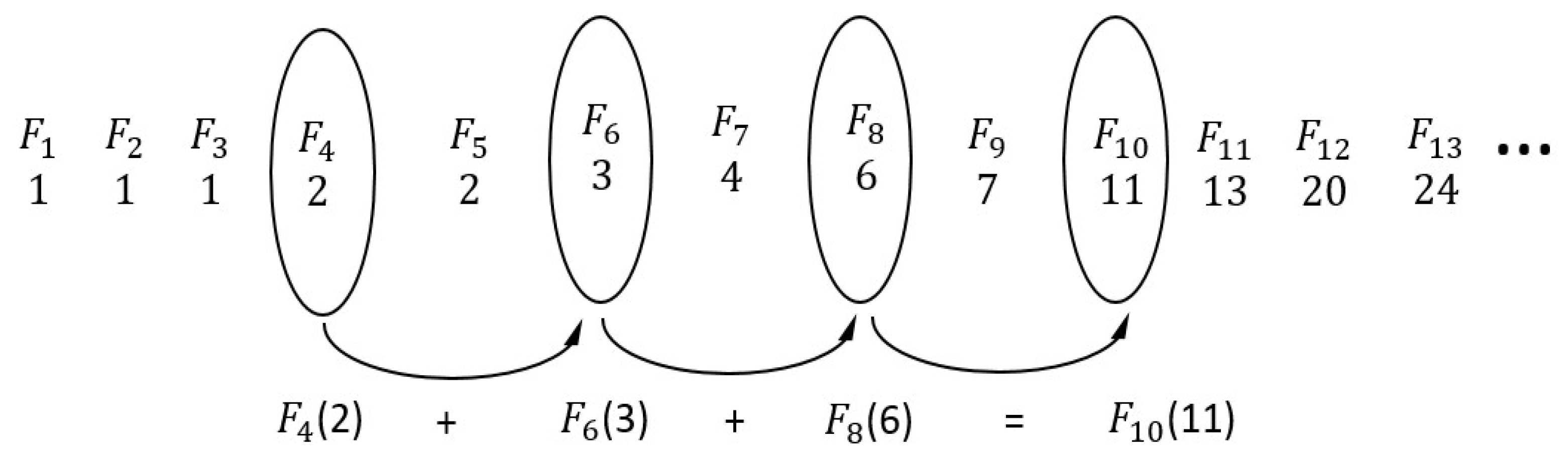
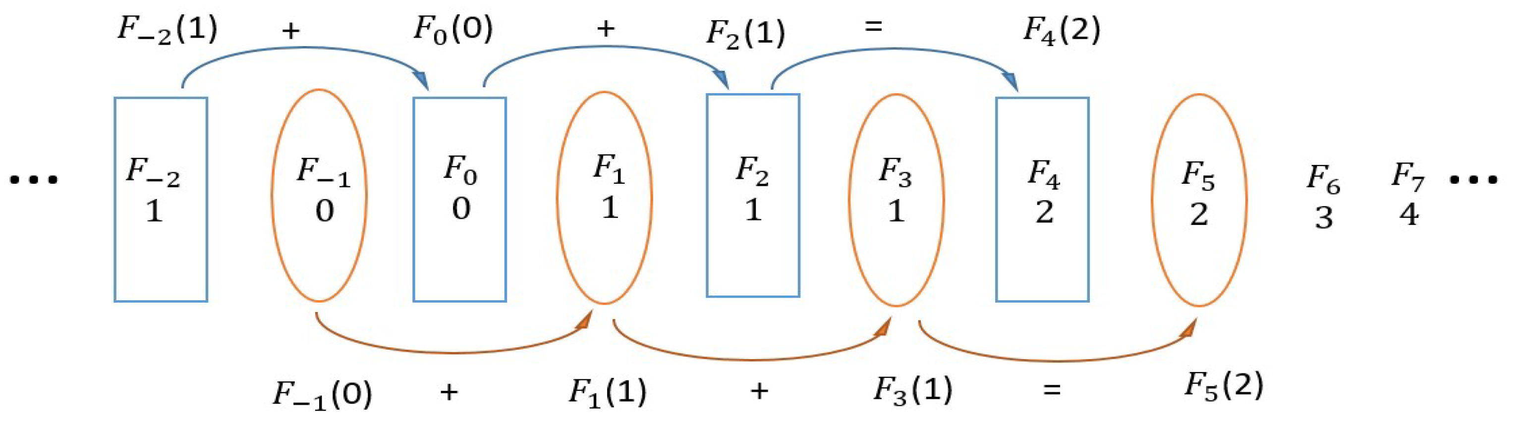
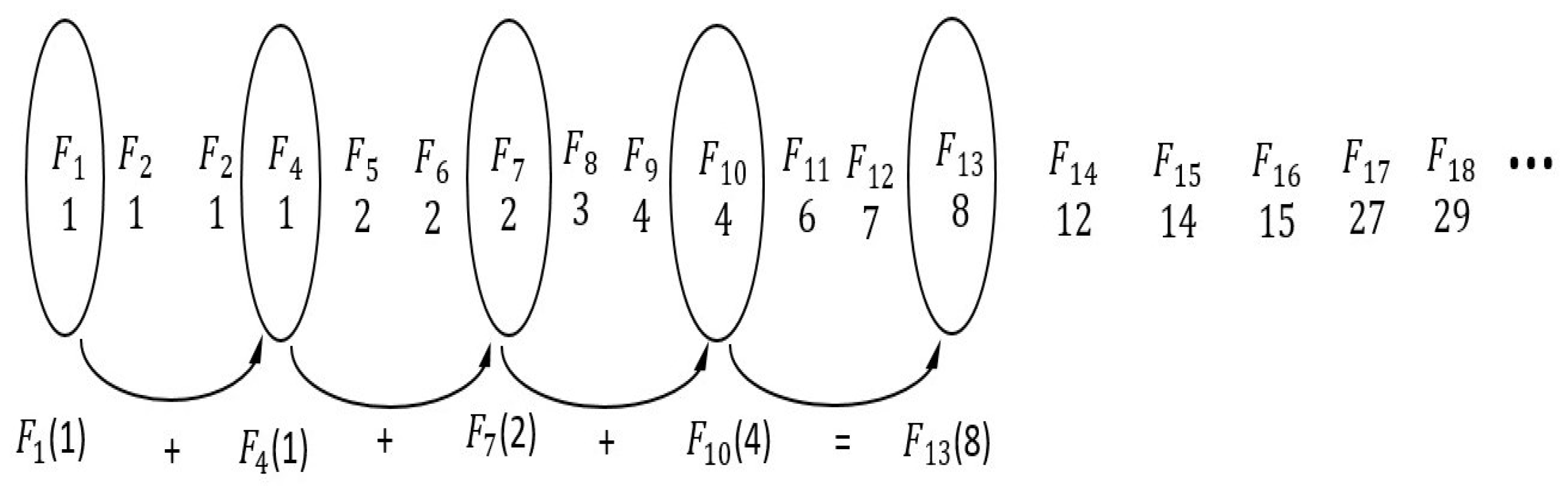
2. Basic Concepts of Fibonacci Sequence

The definitions of Fibonacci numbers in relation to the m-step and generalized m-Fibonacci sequences are provided in this section. Furthermore, we have demonstrated the binomial expansion of the Fibonacci series and the golden ratio of each Fibonacci sequence.

Definition 1.

For any positive integer k, the sequence of Fibonacci numbers is defined by the recurrence relation

$$F_k=\left\{\begin{array}{c}0,k=0\hfill \\ 1,k=1\hfill \\ F_{k-1}+F_{k-2},k\ge 2.\hfill \end{array}\right.$$

(1)

Illustration 1.

Consider the sequence of numbers defined in (1). Then, we have the ratio sequence $F_1/F_0=1$, $F_2/F_1=2$, $F_3/F_2=1.5$, $F_4/F_3=1.67$ and so on. Therefore, we obtain the ratio sequence of the form $\left\{F_1/F_0,F_2/F_1,F_3/F_2,\dots \right\}$. The ratio of two consecutive Fibonacci numbers is called the golden ratio, which is approximately 1.618. That is, it is well known that $\underset{k\to \infty }{lim}{F}_{k+1}/F_k\approx 1.618$ [44].

Definition 2 is a generalized version of Definition 1.

Definition 2

([40]). Let $k\ge 0$, $m\ge 2$ be an integer, and $F_k$ be as defined in (1). Then, the generalized m-Fibonacci sequence is defined as

$$F_k^{(m-1)}=\left\{\begin{array}{c}0,k=0\hfill \\ 1,0<k\le m\hfill \\ {\displaystyle \sum _{r=1}^m}{F}_{k-r},k>m\hfill \end{array}\right.,$$

(2)

and also, the m-step Fibonacci sequence is defined as

$$F^{k,m-1}=\left\{\begin{array}{c}0,k<0\hfill \\ 1,k\in \{1,2\}\hfill \\ {\displaystyle \sum _{r=1}^m}{F}_{k-r},k>2\hfill \end{array}\right..$$

(3)

Applying a similar procedure to Illustration 1, we obtain a unique limit for each sequence given in Definition 2. The limit values for each sequence are stated in

Table 2. Golden ratios of the generalized Fibonacci sequences given in Definition 2.

For $\mathit{m}\ge 2$	List of Sequences	Golden Ratio
$F_k^{\left(1\right)}$	$1,1,2,3,5,8,13,21,34,55,\cdots$	$\underset{k\to \infty }{lim}{F}_{k+1}^{\left(1\right)}/F_k^{\left(1\right)}\approx 1.618$
$F^{k,1}$	$1,1,2,3,5,8,13,21,34,55,\cdots$	$\underset{k\to \infty }{lim}{F}^{k+1,1}/F^{k,1}\approx 1.618$
$F_k^{\left(2\right)}$	$1,1,1,3,5,9,17,31,57,105,\cdots$	$\underset{k\to \infty }{lim}{F}_{k+1}^{\left(2\right)}/F_k^{\left(2\right)}\approx 1.84$
$F^{k,2}$	$1,1,2,4,7,13,24,44,81,\cdots$	$\underset{k\to \infty }{lim}{F}^{k+1,2}/F^{k,2}\approx 1.84$
$F_k^{\left(3\right)}$	$1,1,1,1,4,7,13,25,49,94,\cdots$	$\underset{k\to \infty }{lim}{F}_{k+1}^{\left(3\right)}/F_k^{\left(3\right)}\approx 1.93$
$F^{k,3}$	$1,1,2,4,8,15,29,56,108,\cdots$	$\underset{k\to \infty }{lim}{F}^{k+1,3}/F^{k,3}\approx 1.93$
$F_k^{\left(4\right)}$	$1,1,1,1,1,5,9,17,33,65,\cdots$	$\underset{k\to \infty }{lim}{F}_{k+1}^{\left(4\right)}/F_k^{\left(4\right)}\approx 1.97$
$F^{k,4}$	$1,1,2,4,8,16,31,61,120,\cdots$	$\underset{k\to \infty }{lim}{F}^{k+1,4}/F^{k,4}\approx 1.97$
$F_k^{\left(5\right)}$	$1,1,1,1,1,1,6,11,21,41,81,\cdots$	$\underset{k\to \infty }{lim}{F}_{k+1}^{\left(5\right)}/F_k^{\left(5\right)}\approx 1.98$
$F^{k,5}$	$1,1,2,4,8,16,32,63,125,\cdots$	$\underset{k\to \infty }{lim}{F}^{k+1,5}/F^{k,5}\approx 1.98$
$F_k^{\left(6\right)}$	$1,1,1,1,1,1,1,7,13,25,49,\cdots$	$\underset{k\to \infty }{lim}{F}_{k+1}^{\left(6\right)}/F_k^{\left(6\right)}\approx 1.99$
$F^{k,6}$	$1,1,2,4,8,16,32,64,127,\cdots$	$\underset{k\to \infty }{lim}{F}^{k+1,6}/F^{k,6}\approx 1.99$

, and these limit values are said to be the golden ratio. Note that the m-Fibonacci $\left(say{F}_k^{(m-1)}\right)$ and m-step Fibonacci $\left(say{F}^{k,m-1}\right)$ are not the same.

Lemma 1.

For $n\in \mathbb{N}$ and $k\ge 2n$, the binomial expansion of Fibonacci series is given by

$${ }_n{F}_k=F_{k-n}+{ }_n{C}_1{F}_{k-(n+1)}+{ }_n{C}_2{F}_{k-(n+2)}+\cdots +{ }_n{C}_n{F}_{k-2n},$$

(4)

where ${ }_n{C}_j(j=1,2,\dots ,n)$ represents the constant coefficients of Pascal’s triangle.

Proof. 

Let us consider the Fibonacci equation as

$${ }_1{F}_k=F_{k-1}+F_{k-2}.$$

(5)

Now, replacing k by $k-1$ and $k-2$ in Equation (5), and then substituting the values of $F_{k-1}$ and $F_{k-2}$, respectively, into Equation (5), we obtain

$${ }_2{F}_k=F_{k-2}+2F_{k-3}+F_{k-4}.$$

(6)

Again, replacing k by $k-2$, $k-3$ and $k-4$ in Equation (5), and then substituting the values of $F_{k-2}$, $F_{k-3}$ and $F_{k-4}$, respectively, into (6), we obtain

$${ }_3{F}_k=F_{k-3}+3F_{k-4}+3F_{k-5}+F_{k-6}.$$

(7)

Similarly, proceeding like this up to n times, we arrive at Equation (4). □

3. Coefficients of the Generalized Fibonacci Equation

In this section, we have first determined the coefficients of the generalized m-th Fibonacci equation. From these coefficients, we can deduce a list of sequences that serve as a new kind of Fibonacci sequence with length h. Also, by utilizing the Fibonacci sequence with length h, we have derived several theorems.

Theorem 1.

Let $F_k$ be defined as in (1). For any positive integers n, and $k\ge n+1$, the general form of Fibonacci equation is given by

$${ }_n{F}_k^{\left(1\right)}=a_n{F}_{k-n}+a_{n-1}{F}_{k-(n+1)};a_0=a_1=1.$$

(8)

Here, the coefficients are obtained as $a_n=a_{n-1}+a_{n-2}$.

Proof. 

Equation (1) can be written in the form of

$${ }_1{F}_k^{\left(1\right)}=F_{k-1}+F_{k-2},\mathrm{where}{a}_0=1,a_1=1.$$

(9)

Now, replacing $F_{k-1}$ by $F_{k-2}+F_{k-3}$ in Equation (9), we arrive at

$${ }_2{F}_k^{\left(1\right)}=F_{k-2}+F_{k-3}+F_{k-2},$$

which implies

$${ }_2{F}_k^{\left(1\right)}=2F_{k-2}+F_{k-3},\mathrm{where}{a}_2=2,a_1=1.$$

(10)

Again, replacing $F_{k-2}$ by $F_{k-3}+F_{k-4}$ in Equation (10), we obtain

$${ }_3{F}_k^{\left(1\right)}=3F_{k-3}+2F_{k-4},\mathrm{where}{a}_3=3,a_2=2.$$

(11)

Similarly, we can find the other terms as

$${ }_4{F}_k^{\left(1\right)}=5F_{k-4}+3F_{k-5},\mathrm{where}{a}_4=5,a_3=3.$$

(12)

$${ }_5{F}_k^{\left(1\right)}=8F_{k-5}+5F_{k-6},\mathrm{where}{a}_5=8,a_4=5.$$

(13)

$${ }_6{F}_k^{\left(1\right)}=13F_{k-6}+8F_{k-7},\mathrm{where}{a}_6=13,a_5=8.$$

(14)

By repeatedly replacing the term $F_{k-r}(6\le r\le n)$, and then substituting in the preceding equation n times, we obtain (8). □

Theorem 2.

For any integers $n,m\ge 1$ and $k\ge n+m$, the general form of generalized m-th Fibonacci equation is given by

$${ }_n{F}_k^{\left(m\right)}=\sum _{r=0}^m{a}_{mn-r}{F}_{k-(n+r)}.$$

(15)

Here, the coefficient values of $a_{mn}$, $a_{mn-1}$, $a_{mn-2}$, …, and $a_{mn-m}$ will be

$$\left\{\begin{array}{c}{a}_{mn}={\displaystyle \sum _{r=1}^{m+1}}{a}_{mn-rm}\hfill \\ a_{mn-1}={\displaystyle \sum _{r=1}^{m+1}}{a}_{mn-(rm+1)}\hfill \\ a_{mn-2}={\displaystyle \sum _{r=1}^{m+1}}{a}_{mn-(rm+2)}\hfill \\ ⋮\hfill \\ a_{mn-m}={\displaystyle \sum _{r=1}^{m+1}}{a}_{mn-(rm+m)},\hfill \end{array}\right.$$

where $a_m=1$, $a_{m-1}=1$, …, $a_1=1$, $a_0=1$.

Proof. 

We shall prove this theorem using the induction method. If $m=1$, the proof is given in Theorem 1.

For $m=2$, the Tribonacci equation is

$$F_k^{\left(2\right)}=F_{k-1}+F_{k-2}+F_{k-3}.$$

(16)

The above equation can be written as

$${ }_1{F}_k^{\left(2\right)}=a_2{F}_{k-1}+a_1{F}_{k-2}+a_0{F}_{k-3},\mathrm{where}{a}_2=1,a_1=1,a_0=1.$$

(17)

Replacing $F_{k-1}$ by $F_{k-2}+F_{k-3}+F_{k-4}$ in the above equation, we obtain

$${ }_2{F}_k^{\left(2\right)}=a_4{F}_{k-2}+a_3{F}_{k-3}+a_2{F}_{k-4},\mathrm{where}{a}_4=2,a_3=2,a_2=1.$$

(18)

Again replacing $F_{k-2}$ by $F_{k-3}+F_{k-4}+F_{k-5}$, we have

$${ }_3{F}_k^{\left(2\right)}=a_6{F}_{k-3}+a_5{F}_{k-4}+a_4{F}_{k-5},\mathrm{where}{a}_6=4,a_5=3,a_4=2.$$

(19)

Proceeding like this n times, we obtain

$${ }_n{F}_k^{\left(2\right)}=a_{2n}{F}_{k-n}+a_{2n-1}{F}_{k-(n+1)}+a_{2n-2}{F}_{k-(n+2)},$$

(20)

where $\left\{\begin{array}{c}{a}_{2n}=a_{2n-2}+a_{2n-4}+a_{2n-6}\hfill \\ a_{2n-1}=a_{2n-3}+a_{2n-5}+a_{2n-7}\hfill \\ a_{2n-2}=a_{2n-4}+a_{2n-6}+a_{2n-8}\hfill \end{array}\right.$.

For $m=3$, the Tetranacci equation is $F_k^{\left(3\right)}=F_{k-1}+F_{k-2}+F_{k-3}+F_{k-4}$ and proceeding similar steps from (17) to (19), we obtain the general form as

$${ }_n{F}_k^{\left(3\right)}=a_{3n}{F}_{k-n}+a_{3n-1}{F}_{k-(n+1)}+a_{3n-2}{F}_{k-(n+2)}+a_{3n-3}{F}_{k-(n+3)},$$

(21)

where the coefficients are $\left\{\begin{array}{c}{a}_{3n}=a_{3n-3}+a_{3n-6}+a_{3n-9}+a_{3n-12}\hfill \\ a_{3n-1}=a_{3n-4}+a_{3n-7}+a_{3n-10}+a_{3n-13}\hfill \\ a_{3n-2}=a_{3n-5}+a_{3n-8}+a_{3n-11}+a_{3n-14}\hfill \\ a_{3n-3}=a_{3n-6}+a_{3n-9}+a_{3n-12}+a_{3n-15}\hfill \end{array}\right.$.

Similarly, for $m=m-1$, we obtain

$${ }_n{F}_k^{(m-1)}=a_{(m-1)n}{F}_{k-n}+a_{\left(\right(m-1\left)n\right)-1}{F}_{k-(n+1)}+\dots +a_{(m-1)n-(m-1)}{F}_{k-(n+(m-1\left)\right)},$$

(22)

where the coefficients are $\left\{\begin{array}{c}{a}_{(m-1)n}=a_{(m-1)n-(m-1)}+a_{(m-1)n-2(m-1)}+a_{(m-1)n-3(m-1)}+\cdots +a_{(m-1)n-(m-1)m}\hfill \\ a_{\left(\right(m-1\left)n\right)-1}=a_{(m-1)n-\left(\right(m-1)+1)}+a_{(m-1)n-\left(2\right(m-1)+1)}+\cdots +a_{(m-1)n-\left(\right(m-1)m+1)}\hfill \\ a_{\left(\right(m-1\left)n\right)-2}=a_{(m-1)n-\left(\right(m-1)+2)}+a_{(m-1)n-\left(2\right(m-1)+2)}+\cdots +a_{(m-1)n-\left(\right(m-1)m+2)}\hfill \\ ⋮\hfill \\ a_{\left(\right(m-1\left)n\right)-(m-1)}=a_{(m-1)n-2(m-1)}+a_{(m-1)n-3(m-1)}+\cdots +a_{(m-1)n-\left(\right(m-1)m+(m-1\left)\right)}\hfill \end{array}\right.$.

Hence, the proof completes. □

Taking the coefficients from Theorem 1, we obtain a sequence of the form

$$1,1,2,3,5,8,13,21,34,55,89,\dots$$

(23)

The above sequence is known as the Fibonacci sequence, and is clearly explained in Definition 1.

Theorem 3.

Let $F_{k-2r}=\left\{\begin{array}{c}1,\mathrm{if}k-2r\in \{-2-3n:n\in \mathbb{N}(0\left)\right\}\hfill \\ 0,\mathrm{if}k-2r\notin \{-2-3n:n\in \mathbb{N}(0\left)\right\}\hfill \end{array}\right.$ for $k-2r<0$. Then, for any positive integer k, the h-Tribonacci equation is given by

$$F_{k,2}=F_{k-2}+F_{k-4}+F_{k-6},F_0=0\mathrm{and}{F}_1=1.$$

(24)

Proof. 

Taking the coefficients from Theorem 2 for $m=2$, we have the $F_{k,2}$ sequence as

$$1,1,1,2,2,3,4,6,7,11,13,20,24,\dots$$

(25)

Simply, the proof follows by referring Figure 1 and Figure 2. □

Note 1.

In Figure 1 and Figure 2, the number in the brackets is the value of $F_n$.

Theorem 4.

Let $F_{k-rh}=\left\{\begin{array}{c}1,\mathrm{if}k-rh\in \{-h-(h+1)n:n\in \mathbb{N}(0\left)\right\}\hfill \\ 0,\mathrm{if}k-rh\notin \{-h-(h+1)n:n\in \mathbb{N}(0\left)\right\}\hfill \end{array}\right.$

for $k-rh<0$ and $r>1$. Then, for any positive integers k and h, the generalized h-length Fibonacci equation is given by

$$F_{k,h}=F_{k-h}+F_{k-2h}+F_{k-3h}+F_{k-4h}+\cdots +F_{k-h(h+1)}.$$

(26)

Proof. 

We shall prove this theorem using the Induction method.

For $h=1$, the proof is obvious.

For $h=2$, the proof is provided in Theorem 3.

For $h=3$, taking the coefficients from Theorem 2 for $m=3$, we obtain the sequence of the form $1,1,1,1,2,2,2,3,4,4,6,7,8,\dots$ This sequence can easily obtained by using the h-Tetranacci equation, which is given below.

$$F_{k,3}=F_{k-3}+F_{k-6}+F_{k-9}+F_{k-12}.$$

(27)

From Figure 3, one can clearly find the value of Equation (27). If $k<0$, then Figure 4 yields

Here, the initial conditions are $F_1=F_2=F_3=F_4=1$ and $F_{k-3r}=\left\{\begin{array}{c}1,\mathrm{if}k-3r\in \{-3-4n:n\in \mathbb{N}(0\left)\right\}\hfill \\ 0,\mathrm{if}k-3r\notin \{-3-4n:n\in \mathbb{N}(0\left)\right\}\hfill \end{array}\right.$ for $k-3r<0$.

Similarly, the fourth, fifth, sixth, … sequence can be found by the following equations.

$$F_{k,4}=F_{k-4}+F_{k-8}+F_{k-12}+F_{k-16}+F_{k-20}$$

(28)

$$F_{k,5}=F_{k-5}+F_{k-10}+F_{k-15}+F_{k-20}+F_{k-25}+F_{k-30}$$

(29)

$$⋮$$

$$F_{k,h}=F_{k-h}+F_{k-2h}+F_{k-3h}+F_{k-4h}+F_{k-5h}+\cdots +F_{k-(h+1)h}.$$

(30)

Hence, the proof completes. □

Remark 1.

If $h=1$, then Equation (26) becomes Equation (1).

Theorem 5.

For $n,h\in \mathbb{N}$ and $k\ge 2nh$, the binomial expansion of the h-length Fibonacci equation is given by

$${ }_n{F}_{k,h}=F_{k-nh}+{ }_n{C}_1{F}_{k-(n+1)h}+{ }_n{C}_2{F}_{k-(n+2)h}+\cdots +{ }_n{C}_n{F}_{k-2nh},$$

(31)

where ${ }_n{C}_j(j=1,2,\dots ,n)$ represents the constant coefficients of Pascal’s triangle.

Proof. 

The proof is similar to Lemma 1 by applying the h-Fibonacci equation $(\mathrm{say}{F}_{k,h}=F_{k-h}+F_{k-2h})$. □

4. $\mathcal{H}$-Nacci Sequence: A Generalization

From the coefficients of Theorem 2 for $m=1,2,3,\dots$, we have developed a new kind of Fibonacci sequence, known as the $\mathcal{H}$-Nacci sequence (or generalized Fibonacci sequence with length h). This $\mathcal{H}$-Nacci sequence serves as a generalized form of other Fibonacci-like sequences that already exist.

Definition 3.

For $k,h\in \mathbb{N}$, the generalized $\mathcal{H}$-Nacci sequence is defined by

$$F_{k,h}=\left\{\begin{array}{c}1,\mathit{if}k\in \{-h-(h+1)n:n\in \mathbb{N}(0\left)\right\}\hfill \\ 0,\mathit{if}-\infty <k-\{-h-(h+1)n:n\in \mathbb{N}(0\left)\right\}\le 0\hfill \\ {\displaystyle \sum _{r=1}^{h+1}}{F}_{k-rh},\mathit{if}k\ge 1\hfill \end{array}\right..$$

(32)

Theorem 6.

For $h\in \mathbb{N}$, there exists a real L, such that

$$\underset{r\to \infty }{lim}(F_{r+h,h}/F_{r,h})=L.$$

(33)

Proof. 

Since $\{F_{r-h,h}/F_{r,h}\}$ is a monotonic bounded real sequence, it has an unique limit L. Hence, we say that $(F_{r+h,h}/F_{r,h})\to L$ as $r\to \infty$ for large r. □

Result 1.

If we take $h=1$ in Theorem 6, then Illustration 1 gives the solution.

Illustration 2.

Let $\{1,1,1,2,2,3,4,6,7,11,13,20,\cdots \}$ be the sequence obtained from Equation (32) for $h=2$. Then, we have the ratio sequence $F_{3,2}/F_{1,2}=1$, $F_{4,2}/F_{2,2}=2$, $F_{5,2}/F_{3,2}=2$ and so on. Therefore, we obtain the ratio sequence of the form $\left\{F_{3,2}/F_{1,2},F_{4,2}/F_{2,2},F_{5,2}/F_{3,2},\dots \right\}$. Now, for any arbitrary small number $ϵ$, there exists a natural number N and real L such that distance between ${\left\{F_{r+2,2}/F_{r,2}\right\}}_{r\ge N}$ and L is less than $ϵ$. Hence, $F_{r+2,2}/F_{r,2}\to L$ as $r\to \infty$ for all large r.

Remark 2.

From Illustration 2, we obtain the limit value as $L\approx 1.84$, so that $F_{r+2,2}/F_{r,2}$ tends to $1.84$ as $r\to \infty$ for $r\ge N$.

Illustration 3.

Let $\{1,1,1,1,2,2,2,3,4,4,6,7,8,\cdots \}$ be a sequence of positive integers from Equation (32) for $h=3$ and if $F_{4,3}/F_{1,3}=2$, $F_{5,3}/F_{2,3}=2$, $F_{6,3}/F_{3,3}=2$, …, then we obtain the ratio sequence of the form $\left\{F_{4,3}/F_{1,3},F_{5,3}/F_{2,3},F_{6,3}/F_{3,3},\dots \right\}$. Now, for any arbitrary small number $ϵ$, there exists a natural number N and real L, such that the distance between ${\left\{F_{r+3,3}/F_{r,3}\right\}}_{r\ge N}$ and L is less than $ϵ$. Hence, $F_{r+3,3}/F_{r,3}\to a$ as $r\to \infty$ for all large r.

Remark 3.

From Illustration 3, we obtain the limit value as $L\approx 1.93$, so that $F_{r+3,3}/F_{r,3}$ tends to $1.93$ as $r\to \infty$ for $r\ge N$.

5. Golden Ratio for $\mathcal{H}$-Nacci Sequence

The limit values for each $\mathcal{H}$-Nacci sequence can be determined through Theorem 6, and this is known as the golden ratio. The golden ratios for each sequence and its names are provided in

Table 3. $\mathcal{H}$-Nacci sequences and their golden ratios.

$\mathcal{H}$-Nacci Names	List of $\mathcal{H}$-Nacci Sequence	Golden Ratio
h-Fibonacci	$1,1,2,3,5,8,13,21,34,55,\dots$	$\underset{n\to \infty }{lim}{F}_{n+1,1}/F_{n,1}\approx 1.618$
h-Tribonacci	$1,1,1,2,2,3,4,6,7,11,13,20,\dots$	$\underset{n\to \infty }{lim}{F}_{n+2,2}/F_{n,2}\approx 1.84$
h-Tetranacci	$1,1,1,1,2,2,2,3,4,4,6,7,8,\dots$	$\underset{n\to \infty }{lim}{F}_{n+3,3}/F_{n,3}\approx 1.93$
h-Pentanacci	$1,1,1,1,1,2,2,2,2,3,4,4,4,6,\dots$	$\underset{n\to \infty }{lim}{F}_{n+4,4}/F_{n,4}\approx 1.97$
h-Hexanacci	$1,1,1,1,1,1,2,2,2,2,2,3,4,4,\dots$	$\underset{n\to \infty }{lim}{F}_{n+5,5}/F_{n,5}\approx 1.98$
h-Heptanacci	$1,1,1,1,1,1,1,2,2,2,2,2,2,3,\dots$	$\underset{n\to \infty }{lim}{F}_{n+6,6}/F_{n,6}\approx 1.99$
$⋮$	$⋮$	$⋮$

.

From Table 2 and Table 3, it is clearly shown that the golden ratio for the $\mathcal{H}$-Nacci sequence and the already existing sequence are exactly same. For the already existing model, the golden ratio can be obtained by taking the ratio between two consecutive numbers, but in the case of the $\mathcal{H}$-Nacci sequence, we find the golden ratio by taking the ratio for two consecutive numbers with length h, where $h\in \{1,2,3,\dots \}$.

6. The Generalization of Other Fibonacci-like Sequence

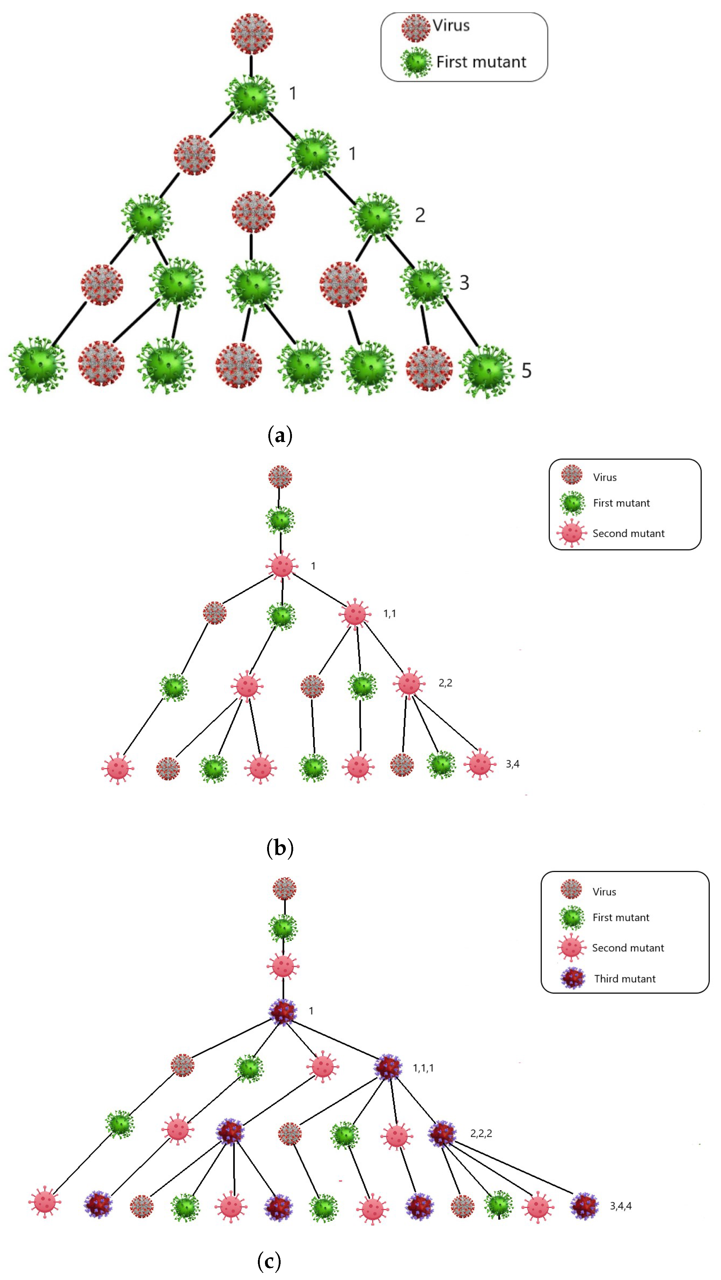
This section will demonstrate how each existing Fibonacci sequence can be generalized using the $\mathcal{H}$-Nacci sequence. By taking $h=1$ in Equation (32), we obtain the sequence given in (23).

Taking $h=2$ in (32) yields (25). From (25), we split the h-Tribonacci sequence into two sequences, such as $F_{1,2},F_{3,2},F_{5,2},F_{7,2},\dots$ and $F_{2,2},F_{4,2},F_{6,2},F_{8,2},\dots$. The two sequences can be expressed as the form

$$1,1,2,4,7,13,24,44,81,149,280,\dots (\mathrm{Tribonacci}m\text{-step}\mathrm{sequence})$$

(34)

$$1,2,3,6,11,20,37,68,125,230,423,\dots (\mathrm{Narayana}\mathrm{Tribonacci}\mathrm{sequence})$$

(35)

For $h=3$, we obtain the h-Tetranacci sequence given in (27). Now, splitting the h-Tetranacci sequence into three forms, such as $F_{1,3},F_{4,3},F_{7,3},F_{10,3},\dots$, $F_{2,3},F_{5,3},F_{8,3},F_{11,3},\dots$, and $F_{3,3},F_{6,3},F_{9,3},F_{12,3},\dots$, we obtain

$$1,1,2,4,8,15,29,56,108,208,401,773,\dots (\mathrm{Tetranacci}m\text{-step}\mathrm{sequence})$$

(36)

$$1,2,3,6,12,23,44,85,164,316,609,\dots \left(\text{Padovan-Perrin}\mathrm{Tetranacci}\mathrm{sequence}\right)$$

(37)

$$1,2,4,7,14,27,52,100,193,372,717,\dots (\mathrm{Narayana}\mathrm{Tetranacci}\mathrm{sequence})$$

(38)

Similarly, from the h-Pentanacci sequence, one can split the sequence into four forms, each of which will match any of the sequences shown in Table 1. Therefore, by repeating this for every $\mathcal{H}$-Nacci sequence, we obtain lot of sequences, each of which must match the sequence that is listed in Table 1. Thus, we refer to the $\mathcal{H}$-Nacci sequence as the generalization of other sequences that already exist.

7. Virus Mutation

Mutation is the ultimate cause of all genetic variation [45,46,47]. Because it generates a new DNA sequence for a specific gene, mutation is essential as the first stage of evolution, because it results in the creation of a new allele. A mutation is a change in our DNA sequence that can be brought on by environmental factors like cigarette smoke and UV light, or mistakes made when the DNA is copied.

Many mutations are inactive, meaning they have no impact on the organism in which they occur. Certain mutations are advantageous and increase fitness. One illustration is a mutation that causes bacteria to become resistant to antibiotics. Some mutations, such as those that lead to genetic diseases, are harmful and reduce fitness; such types of viruses are flu, coronavirus, etc.

Usually, DNA and RNA both undergo the mutation process. The structure of DNA and RNA is given in Figure 5. Single-stranded viruses change more quickly than double-stranded viruses, and the size of the genome appears to be negatively correlated with the rate of mutation. DNA is a double-stranded molecule with a lengthy chain of nucleotides. A single-stranded molecule, called RNA, contains a shorter chain of nucleotides than other molecules. DNA is self-replicating; it duplicates itself. RNA cannot replicate on its own. Compared to DNA systems, RNA viruses exhibit higher mutation rates. A virus that has undergone one or more mutations is known as a “variant” of the parent virus [48]. To have a better understanding, we will look at how the virus has mutated in coronavirus.

8. Fibonacci Numbers in Virus Mutation

Each Fibonacci sequence has an unique character. By utilizing the virus mutation process, we clearly explain the characterization of each Fibonacci sequence given in Definitions 2 and 3. In this section, we analyze the key benefits of the generalized m-Fibonacci, m-step Fibonacci and $\mathcal{H}$-Nacci sequence in terms of the virus mutation process.

(i)

Generalized m-Fibonacci sequence:

We can clearly understand from Figure 6 that the parent virus has undergone three mutations: the first mutation in Figure 6a, the second mutation in Figure 6b, and the third mutation in Figure 6c. While counting the number for each spreadness, we obtain the sequences of the form $1,1,2,3,5,8,\cdots$, $1,1,1,3,5,9,\cdots$ and $1,1,1,1,4,7,13,\cdots$. As a result, the generalized m-Fibonacci sequence can be used to calculate the total number of viral spread over all types.

(ii)

m-step Fibonacci sequence:

In this case, we have just provided the numbers for the last mutant virus. As a result, we obtain the sequences $1,1,2,3,5,8,\cdots$ from Figure 7a, $1,1,2,4,7,13,\cdots$ from Figure 7b, and $1,1,2,4,8,15,\cdots$ from Figure 7c, which is obviously shown in Figure 7. With this kind of sequence, it is simple to determine the spreading ratio of the final mutant virus.

(iii)

$\mathcal{H}$-Nacci sequence:

In this case, we have provide the numbers for each mutant virus from the finally mutated virus. From Figure 8, we obtain the sequence $1,1,2,3,4,5,\cdots$ from Figure 8a, the sequence $1,1,1,2,2,3,4,\cdots$ from Figure 8b, and the sequence $1,1,1,1,2,2,2,3,$$4,4,\cdots$ from Figure 8c. The spreading ratio of the first and second mutant viruses is shown in Figure 8a,b in two separate numbers, and in Figure 8c, it gives three separate numbers for the first, second, and third mutant viruses. Because of this, it is simple to determine the spreading ratios of the first, second, and third mutations separately using this sequence.

Therefore, Figure 6 gives us the total number of mutant viruses, while Figure 7 gives us the total number of the final mutant virus. However, the sequence from Figure 8 helps us to find the overall number of each mutant virus.

9. Fibonacci Risk Modeling

Risk ratings are always based on comparison. As an illustration, it is dangerous to jump off a moving train. The most rational course of action, though, is to jump if the train is about to crash off a cliff. Risk cannot be measured in absolute terms; instead, it can only be compared to other options. Therefore, each activity is not always risk-free if the risk value is 0. We can reduce the activity risk if the risk value is zero. Similarly, a risk value of 1 just indicates that we can increased the activity risk.

9.1. Fibonacci Risk Formula

The Fibonacci series is a set of numbers where each number is the sum of the two before it, apart from the fact that the first two values are always specified as 1. This definition produces the numbers $1,1,2,3,5,8,13,\cdots$ in a sequence.

To find the risk factor, let us first provide a risk value to each risk level by color coding. A risk factor is nothing but one’s risk value. Therefore, it is entirely our choice to choose the risk value for varying danger level. The level of risk factor is given in Figure 9.

The critical risk formula is

$$Risk={\displaystyle \frac{R{L}_L\times N_L+R{L}_{ML}\times N_{ML}+R{L}_M\times N_M+R{L}_{MH}\times N_{MH}+R{L}_C\times N_C}{R{L}_C\times N}},$$

(39)

where $N=N_L+N_{ML}+N_M+N_{MH}+N_C$ and other parameters are mentioned in

Table 4. The parameters and description of Equation (39).

Parameters	Description
$R{L}_L$	Low risk level activity
$R{L}_{ML}$	Medium-Low risk level activity
$R{L}_M$	Medium risk level activity
$R{L}_{MH}$	Medium-High risk level activity
$R{L}_C$	High risk (critical) level activity
$N_L$	Number of Low risk activities
$N_{ML}$	Number of Medium-Low risk activities
$N_M$	Number of Medium risk activities
$N_{MH}$	Number of Medium-High risk activities
$N_C$	Number of High risk (critical) activities

.

Let us assume any five consecutive numbers from the Fibonacci sequence as risk values, such as $144,233,377,610,987$. If $R{L}_L$ is the low level risk activity, then the other risk factors are:

$$R{L}_{ML}=\varphi R{L}_L$$

(40)

$$R{L}_M={\varphi }^{2}R{L}_L$$

(41)

$$R{L}_{MH}={\varphi }^{3}R{L}_L$$

(42)

$$R{L}_C={\varphi }^{4}R{L}_L$$

(43)

Substituting Equations (40)–(43) into Equation (39), we obtain

$$Risk={\displaystyle \frac{R{L}_L{N}_L+\varphi R{L}_L{N}_{ML}+{\varphi }^{2}R{L}_L{N}_M+{\varphi }^{3}R{L}_L{N}_{MH}+{\varphi }^{4}R{L}_L{N}_C}{{\varphi }^{4}R{L}_{L}N}},$$

(44)

which is same as

$$Risk={\displaystyle \frac{N_L+\varphi N_{ML}+{\varphi }^2{N}_M+{\varphi }^3{N}_{MH}+{\varphi }^4{N}_C}{{\varphi }^{4}N}}.$$

(45)

Now, substituting the $\varphi$, ${\varphi }^2$, ${\varphi }^3$, ${\varphi }^4$ values into the above equation, it becomes

$$Risk={\displaystyle \frac{N_L+1.62\times N_{ML}+2.62\times N_M+4.24\times N_{MH}+6.85\times N_C}{6.85\times N}}.$$

(46)

This risk model is referred to as the Fibonacci risk model.

9.2. Criticality Risk Values

If all of the activities are $R{L}_C$, the criticality risk’s maximum value reaches 1.0. Therefore, $N_L$, $N_{ML}$, $N_M$, and $N_{MH}$ are zero, and $N_C$ equals N:

$$Risk={\displaystyle \frac{0+1.62\times 0+2.62\times 0+4.24\times 0+6.85\times N}{6.85\times N}}=1.$$

(47)

When all of the activities are $R{L}_L$, the criticality risk has a minimum value of $R{L}_L$ over $R{L}_C$. Therefore, $N_{ML}$, $N_M$, $N_{MH}$ and $N_C$ are zero, and $N_L$ equals N:

$$Risk={\displaystyle \frac{N+1.62\times 0+2.62\times 0+4.24\times 0+6.85\times 0}{6.85\times N}}={\displaystyle \frac{1}{6.85}}=0.15.$$

(48)

Thus, 0.15 is the lowest possible risk value. There can never be zero criticality risk. The risk factor should never be zero; this is not always a bad thing.

9.3. Activity Risk

Broad categories of risk are used in the criticality risk model. For example, if you define large number of activities, we can use this activity risk model. Compared to the criticality risk, this model is far more discrete and accurate. The activity risk formula is

$$Risk=1-{\displaystyle \frac{F_1+\cdots +F_N}{F_N\times N}}=1-{\displaystyle \frac{{\displaystyle \sum _{r=1}^N}{F}_r}{F_N\times N}}.$$

(49)

where $F_r$ represents the rth-activity, N represents the total number of activities, and $F_N$ represents the maximum activity value.

9.4. Activity Risk Values

When all activities are critical, the activity risk model is undefinable. This model approaches 1 if the greater activity value is almost equivalent to the specified activities

$$Risk\approx 1-{\displaystyle \frac{M}{M\times N}}=1-{\displaystyle \frac{1}{N}}\approx 1.$$

(50)

When all activities have the same level of M, then the minimum value of the activity risk is 0. That is,

$$Risk=1-{\displaystyle \frac{{\displaystyle \sum _{i=1}^N}M}{M\ast N}}=1-{\displaystyle \frac{M\times N}{M\times N}}=0.$$

(51)

Although activity risk can theoretically approach zero, in reality, every risk has some non-zero amount of risk value.

Example 1.

Assuming the critical value as the 40-th activity ($N=40$) in the Fibonacci sequence, Equation (49) becomes

$$Risk=1-{\displaystyle \frac{{\displaystyle \sum _{r=1}^{40}}{F}_r}{F_{40}\times 40}}=1-{\displaystyle \frac{1+1+2+\cdots +102334155}{102334155\times 40}}=0.94.$$

(52)

Therefore, for larger N (critical), the risk value will approach to 1. If there is very low activity from the Fibonacci sequence, then Equation (49) becomes

$$Risk=1-{\displaystyle \frac{{\displaystyle \sum _{r=1}^2}{F}_r}{F_2\times 2}}=1-{\displaystyle \frac{1+1}{1\times 2}}=1-1=0.$$

(53)

Hence, Equations (50) and (51) are verified.

9.5. Risk Activity for Tribonacci Sequence

In this section, we are going to compare the maximum and minimum risk factor for Tribonacci sequence. Let us assume the critical value as 30-th activity in the Tribonacci sequence; then, Equation (49) becomes

$$Risk=1-{\displaystyle \frac{F_1+F_2+F_3+\cdots +F_{30}}{F_{30}\times 30}}.$$

(54)

Therefore, we obtain three cases, such as

$$Them-FibonacciactivityRisk=1-{\displaystyle \frac{1+1+1+\cdots +20603361}{20603361\times 30}}=0.93.$$

(55)

$$Them-stepFibonacciactivityRisk=1-{\displaystyle \frac{1+1+2+\cdots +24649061}{24649061\times 30}}=0.93.$$

(56)

$$The\mathcal{H}-NacciactivityRisk=1-{\displaystyle \frac{1+1+1+\cdots +35890}{35890\times 30}}=0.92.$$

(57)

From Equations (55)–(57), we say the risk factor is approximately approaching one. Thus, if the N value is much larger, then the activity becomes high in terms of criticality. Now, for a lower activity, Equation (49) becomes

$$Them-FibonacciactivityRisk=1-{\displaystyle \frac{1+1+1}{1\times 3}}=0.$$

(58)

$$Them-stepFibonacciactivityRisk=1-{\displaystyle \frac{1+1}{1\times 2}}=0.$$

(59)

$$The\mathcal{H}-NacciactivityRisk=1-{\displaystyle \frac{1+1+1}{1\times 3}}=0.$$

(60)

Hence, we obtain the minimum value. But the minimum value must be a non-zero value. The above three sequences are approaching the same risk factor, and thus we say the $\mathcal{H}$-Nacci sequence risk factor is equivalent to the already existing generalized Fibonacci sequence. The same procedure is used to find other Fibonacci sequence maximum and minimum risk factor.

9.6. Risk Metrics

Maintain risk at 0.2 to 0.75: Never allow for excessive risk values in your activity. A risk value of zero or one is obviously meaningless. Since the criticality risk model cannot be used for values lower than 0.15, the lower bound for any activity should be rounded from 0.15 up to 0.2. While compressing the activity, you should stop before the risk reaches one. It is still high risk, even with a risk value of 0.9 or 0.85. For the sake of consistency, if the bottom quarter of risk values between 0 and 0.15 is forbidden, you should stay away from the top quarter of risk values between 0.8 and 1.

(i)

Reduce compression to 0.5: a risk of 0.5 is the optimal decompression target, since it aims to reduce the risk to its lowest possible level.

(ii)

Do not decompress too much: decompression above the decompression range has a negative value, and over-decompression increases the danger.

(iii)

Normal solutions should not exceed 0.75: if a risk of 0.3 is the lower bound for all solutions, then a risk of 0.75 is the upper bound for a normal solution. High-risk normal solutions should always be decompressed.

As a result, if we take the appropriate precautions before the risk factor exceeds the maximum value, we can control the spread of disease; otherwise, the spread would become uncontrollable.

10. Conclusions

In this paper, we developed a new type of sequence, named the $\mathcal{H}$-Nacci sequence. This sequence behaves in the same way that every other Fibonacci and Fibonacci-like sequence does. Following that, we applied the $\mathcal{H}$-Nacci sequence to the virus mutation process in order to determine the spreadness of a mutant virus. In addition, we developed the Fibonacci risk factor model to calculate the maximum and minimum risk values of the $\mathcal{H}$-Nacci sequence. Here, if the risk factor is between $0.2$ to $0.75$, we can control the virus transmission by taking the safeguards. If the risk factor is between $0.8$ and 1, the virus transmission will be extremely harmful. Likewise, if the risk factor exceeds 1, the virus transmission becomes uncontrollable.

References

1. Blankenship, R.A. The Golden Ratio and Fibonacci Sequence in Music. Ph.D. Thesis, Ohio Dominican University, Columbus, OH, USA, 2021. [Google Scholar]
2. Debnath, L. A short history of the Fibonacci and golden numbers with their applications. Int. J. Math. Educ. Sci. Technol. 2011, 42, 337–367. [Google Scholar] [CrossRef]
3. Dunlap, R.A. The Golden Ratio and Fibonacci Numbers; World Scientific: Singapore, 1997. [Google Scholar]
4. Ilić, I.; Stefanović, M.; Sadiković, D. Mathematical Determination in Nature—The Golden Ratio. Acta Med. Median. 2018, 57, 124. [Google Scholar] [CrossRef]
5. Letchumanan, S.; Idris, R. Application of fibonacci series, golden proportions and golden rectangle to human hand using statistical analysis. Univ. Malays. Teren. J. Undergrad. Res. 2020, 2, 31–40. [Google Scholar] [CrossRef]
6. Grigas, A. The Fibonacci Sequence: Its History, Significance, and Manifestations in Nature. Ph.D. Thesis, Liberty University, Lynchburg, VA, USA, 2013. [Google Scholar]
7. Kalman, D.; Mena, R. The Fibonacci numbers—Exposed. Math. Mag. 2003, 76, 167–181. [Google Scholar]
8. García-Máynez, A.; Acosta, A.P. A method to construct Generalized Fibonacci Sequences. J. Appl. Math. 2016, 2016, 4971594. [Google Scholar] [CrossRef]
9. Falcon, S. Generalized (k,r)-Fibonacci numbers. Gen. Math. Notes 2014, 25, 148–158. [Google Scholar] [CrossRef]
10. Trojovský, P. On terms of generalized Fibonacci sequences which are powers of their indexes. Mathematics 2019, 7, 700. [Google Scholar] [CrossRef]
11. Cohn, J.H. Square fibonacci numbers. In Exploring University Mathematics; Pergamon: Oxford, UK, 1967; pp. 69–82. [Google Scholar]
12. Koshy, T. Fibonacci and Lucas Numbers with Applications; John Wiley & Sons: Hoboken, NJ, USA, 2019; Volume 2. [Google Scholar]
13. Singh, B.; Sisodiya, K.; Ahmad, F. On the Products of k-Fibonacci Numbers and k-Lucas Numbers. Int. J. Math. Math. Sci. 2014, 2014, 505798. [Google Scholar] [CrossRef]
14. Falcon, S.; Plaza, Á. The k-Fibonacci sequence and the Pascal 2-triangle. Chaos Solitons Fractals 2007, 33, 38–49. [Google Scholar] [CrossRef]
15. Falcon, S.; Plaza, A. On k-Fibonacci numbers of arithmetic indexes. Appl. Math. Comput. 2009, 208, 180–185. [Google Scholar] [CrossRef]
16. Holliday, S.H.; Komatsu, T. On the sum of reciprocal generalized Fibonacci numbers. Integers 2011, 11, 441–455. [Google Scholar] [CrossRef]
17. Marques, D. On the spacing between terms of generalized Fibonacci sequences. Colloquium Mathematicum 2014, 2, 267–280. [Google Scholar] [CrossRef]
18. Bravo, J.J.; Gómez, C.A.; Luca, F. On the distance between generalized Fibonacci numbers. Colloq. Math 2015, 140, 107–118. [Google Scholar] [CrossRef]
19. Shannon, A.G.; Horadam, A.F. Generalized Fibonacci number triples. Am. Math. Mon. 1973, 80, 187–190. [Google Scholar] [CrossRef]
20. Frontczak, R. Relations for generalized Fibonacci and Tribonacci sequences. Notes Number Theory Discret. Math. 2019, 25, 178–192. [Google Scholar] [CrossRef]
21. Marques, D.; Togbé, A. Perfect powers among Fibonomial coefficients. Comptes Rendus Math. 2010, 348, 717–720. [Google Scholar] [CrossRef]
22. Bacani, J.B.; Rabago, J.F.T. On generalized Fibonacci numbers. arXiv 2015, arXiv:1503.05305. [Google Scholar] [CrossRef]
23. Luca, F.; Shorey, T.N. Diophantine equations with products of consecutive terms in Lucas sequences. J. Number Theory 2005, 114, 298–311. [Google Scholar] [CrossRef]
24. Gu, A.; Xu, Y. The research of the generalized Fibonacci sequence-based propagation. Phys. Procedia 2012, 24, 1737–1741. [Google Scholar] [CrossRef]
25. Dundar, F.S. COVID-19 and the fibonacci numbers. In Proceedings of the 9th International Eurasian Conference on Mathematical Sciences and Applications, Skopje, North Macedonia, 25–28 August 2020; p. 74. [Google Scholar]
26. Persaud, D.; O’Leary, J.P. Fibonacci series, golden proportions, and the human biology. Austin J. Surg. 2015, 2, 1066. [Google Scholar]
27. Dosal-Trujillo, L.A.; Galeana-Sánchez, H. The Fibonacci numbers of certain subgraphs of circulant graphs. AKCE Int. J. Graphs Comb. 2015, 12, 94–103. [Google Scholar] [CrossRef]
28. Prodinger, H.; Tichy, R. Fibonacci numbers of graphs. Fibonacci Q. 1982, 20, 16–21. [Google Scholar]
29. Szynal-Liana, A.; Włoch, I.; Liana, M. Some identities for generalized Fibonacci and Lucas numbers. AKCE Int. J. Graphs Comb. 2020, 17, 324–328. [Google Scholar] [CrossRef]
30. Włoch, A. On generalized Fibonacci numbers and k-distance Kp-matchings in graphs. Discret. Appl. Math. 2012, 160, 1399–1405. [Google Scholar]
31. Dasdemir, A. On the Pell, Pell-Lucas and modified Pell numbers by matrix method. Appl. Math. Sci. 2011, 5, 3173–3181. [Google Scholar]
32. Catarino, P.; Campos, H. Incomplete k-Pell, k-Pell-Lucas and modi fied k-Pell numbers. Hacet. J. Math. Stat. 2017, 46, 361–372. [Google Scholar]
33. Falcón, S. Binomial Transform of the Generalized k-Fibonacci Numbers. Commun. Math. Appl. 2019, 10, 643. [Google Scholar] [CrossRef]
34. Kwon, Y. Binomial transforms of the modified k-Fibonacci-like sequence. arXiv 2018, arXiv:1804.08119. [Google Scholar]
35. Leyendekkers, J.V.; Shannon, A.G. Primes within generalized Fibonacci sequences. Notes Number Theory Discret. Math. 2015, 21, 56–63. [Google Scholar]
36. Noe, T.D.; Post, J.V. Primes in Fibonacci n-step and Lucas n-step sequences. J. Integer. Seq. 2005, 8, 4. [Google Scholar]
37. Rexma Sherine, V.; Gerly, T.G.; Britto Antony Xavier, G.; Abisha, A. Comparative Analysis on Virus Mutation with Fibonacci Numbers. J. Comput. Math. 2023, 7, 61–72. [Google Scholar] [CrossRef]
38. Singh, B.; Bhadouria, P.; Sikhwal, O.; Sisodiya, K. A formula for Tetranacci-like sequence. Gen. Math. Notes 2014, 20, 136–141. [Google Scholar]
39. Soykan, Y. Summing formulas for generalized Tribonacci numbers. Univers. J. Math. Appl. 2020, 3, 1–11. [Google Scholar] [CrossRef]
40. Soykan, Y. Binomial transform of the generalized Tribonacci sequence. Asian Res. J. Math. 2020, 16, 26–55. [Google Scholar] [CrossRef]
41. Soykan, Y. On generalized Narayana numbers. Int. J. Adv. Appl. Math. Mech. 2020, 7, 43–56. [Google Scholar]
42. Soykan, Y. A Study on Sum Formulas for Generalized Tetranacci Numbers: Closed Forms of the Sum Formulas k = 0 n kWk and k = 1 n kW−k. Asian J. Adv. Res. Rep. 2021, 15, 68–85. [Google Scholar] [CrossRef]
43. Taşyurdu, Y. Binomial Transforms of Generalized Fibonacci-Like Sequences. Int. J. Math. Trends Technol.-IJMTT 2018, 64, 59–64. [Google Scholar] [CrossRef]
44. Fibonacci Sequence. Available online: https://www.britannica.com/science/Fibonacci-number (accessed on 28 August 2024).
45. University of California Museum of Paleontology. Evolution from a Virus’s View. December 2007. Available online: https://evolution.berkeley.edu/evo-news/evolution-from-a-viruss-view/ (accessed on 1 October 2018).
46. CDC. Types of Influenza Viruses. Available online: https://www.cdc.gov/flu/about/viruses/types.htm (accessed on 30 March 2023).
47. CDC. How the Flu Virus Can Change: Shift and Drift. Available online: https://www.cdc.gov/flu/about/viruses/change.htm (accessed on 12 December 2022).
48. World Health Organization. Coronavirus Disease (COVID-19): Variants of SARS-COV-2, 20 November 2023. Available online: https://www.who.int/news-room/questions-and-answers/item/coronavirus-disease-(covid-19)-variants-of-sars-cov-2 (accessed on 20 November 2023).
Figure 1. h-Tribonacci sequence.
Mathematics 12 02695 g001
Figure 2. h-Tribonacci sequence with initial condition.
Mathematics 12 02695 g002
Figure 3. h-length Fibonacci sequence.
Mathematics 12 02695 g003
Figure 4. h-length Fibonacci sequence with initial condition.
Mathematics 12 02695 g004
Figure 5. Structure of RNA and DNA.
Mathematics 12 02695 g005
Figure 6. Generalized m-Fibonacci sequence. (a) Fibonacci sequence; (b) Tribonacci sequence; (c) Tetranacci sequence.
Mathematics 12 02695 g006
Figure 7. Generalized m-step Fibonacci sequence. (a) Fibonacci sequence; (b) Tribonacci sequence; (c) Tetranacci sequence.
Mathematics 12 02695 g007
Figure 8. H -Nacci sequence. (a) Fibonacci sequence; (b) Tribonacci sequence; (c) Tetranacci sequence.
Mathematics 12 02695 g008
Figure 9. Level of risk.
Mathematics 12 02695 g009