A Spatial Agent-Based Model for Studying the Effect of Human Mobility Patterns on Epidemic Outbreaks in Urban Areas

Abstract

The epidemic outbreaks of the last two decades have led governments to rely more on computational tools for establishing protection policies. Computational approaches to modeling epidemics traditionally rely on compartmental models, network models, or agent-based models (ABMs); however, each approach has its limitations, ranging from reduced realism to lack of tractability. Furthermore, the recent literature emphasizes the importance of points of interest (POIs) as sources of population mixing and potential outbreak hotspots. In response, this study proposes a novel urban spatial ABM validated using our augmented SICARQD epidemic model. To replicate daily activities more accurately, the urban area is divided into a matrix of points of interest (POIs) with agents that have unique paths that only permit infectious transmission within POIs. Our results provide a qualitative assessment of how urban characteristics and individual mobility patterns impact the infected population during an outbreak. That is, we study how population density, the total number of POIs (where the population concentrates), the average number of POIs visited by an agent, the maximum travel distance from the home location, and the quarantine ratio impact the dynamics of an outbreak. Our ABM simulation framework offers a valuable tool for investigating and controlling infectious disease outbreaks in urban environments with direct applicability to global policy makers.

1. Introduction

The dynamics of recent epidemics such as H1N1, SARS, and COVID-19 have been a significant challenge and top public health priority for many governments around the world [1,2,3]. Traditional epidemiological approaches employ compartmental models that categorize the population based on economic and demographic factors, among others. Despite the lack of complexity in individual behavior, these models have been shown to be effective in the formation and shaping of public health policies [4,5,6].

Most approaches in computational epidemics use compartmental models (analytical approach), complex network models, agent-based models (ABMs), or hybrid solutions. The sole usage of compartmental models offers reduced realism and tractability since all agents interact with other agents without any geo-spatial restrictions, omitting the complexity of human organization [6,7,8]. Network models solve this problem, as nodes only interact with their neighbors, but it is the infection that must spread to static node locations, instead of allowing nodes to move as in the case of dense urban environments [9,10]. More recently, agent-based models (ABMs) have become a powerful computational tool for the study of infectious disease outbreaks [11,12,13,14,15].

Unlike traditional approaches, such as compartmental models or network models, ABMs offer a high degree of realism by allowing agents to move freely and interact in a dynamic environment. This makes ABMs especially useful in modeling complex urban environments, where populations are dense and mobility patterns play a critical role in the spread of disease [16]. During the beginning of the COVID-19 pandemic, ABMs were successfully used in exchange for simpler compartmental models, such as the SIR and SIS [17,18].

Nevertheless, many ABMs also lack tractability, as agents are permitted to move anywhere and interact anywhere in the system. To this end, the recent literature has shown the increased importance of points of interest (POIs) as the main sources of population mixing and therefore outbreak hotspots [19,20,21]. In other words, it turns out to be more realistic to track human interaction inside POIs only and control the epidemic by limiting access to, or entirely closing, POIs during outbreaks.

Authors Chang et al. [19] showed that a fraction of POIs account for the majority of infections and that restricting POI occupancy is more effective than uniformly reducing mobility. By contrast, the authors use an SEIR epidemic model that cannot account for quarantine and patient recurrence as our SICARQD ($Susceptible - Incubating - Contagious - Aware - Recovered - Quarantined - Dead$) model [22]. The study in [11] by Hackl et al. concentrated on the Zurich (CH) transport network and used a SIR model to explain the dynamics of influenza. Conversely, our ABM provides a general framework for testing customizable urban areas and makes use of a more detailed epidemic model. In [14], authors Zhuge et al. created a hybrid ABM–social network model which establishes friendships between agents based on similarity and geographic information; their model is general purpose but lacks the mobility paradigm for agents. In [20], authors Li et al. provided a statistical study on population flow for POIs for 16 US cities, and showed which categories of POIs were more affected by quarantine. Authors Nian et al. [21] studied the relationship between residents’ mobility, POIs, and social activities from the perspective of taxi travel during COVID-19; their conclusions focused on the recovery of public transport in megacities during the post-epidemic period. Finally, we mention the study by Mao et al. [23], in which the authors employed the SLIR epidemic model for H1N1 and created an ABM for the Buffalo region (USA) with its local businesses (POIs); the authors concluded that certain POIs are critical in spreading the disease.

In light of these recent developments, we propose an urban spatial ABM that replicates the daily mobility of an average individual as much as possible. Specifically, the urban area is divided into a matrix of equidistant POIs, and all agents will have a unique random path of POIs to follow from and back to their home location. Agent interactions that trigger infectious transmission will only be possible inside a POI. In other words, two agents need to be at the same time and at the same POI to be able to transmit an airborne viral infection between each other.

The main motivation of this study is to define a general purpose, customizable, and computationally efficient urban spatial agent-based model which uses a points-of-interest (POIs) matrix as relevant interaction points for the spread of infectious diseases, opinion, innovation, rumors, etc. In terms of originality, agents move independently between a controlled number of POIs in their daily routine and may be restricted to move inside a variable area around their home location. Infection may only occur within POIs, reducing computational complexity from $O\left(A^2\right)$ ($Agent{s}^2$) to $O\left(AP\right)$ ($Agents·POIs$). Moreover, in this study, we focus on epidemic outbreaks and how their dynamics can be influenced by population density, the number of urban POIs, the average number of POIs visited by an agent, the maximum travel distance from the home location, and the impact of the quarantine ratio. To this end, we incorporate our previously validated SICARQD epidemic model [22], which allows patient quarantine and relapse, and supports three stages of infection.

In addition to detailing the urban spatial ABM, our study aims to answer the following questions relevant to epidemic outbreaks:

• How does population (density) in an urban environment affect outbreak dynamics?
• How does the number of population accumulation points (POIs) scale with the impact of an outbreak?
• How do mobility restrictions (reducing the maximum travel distance and the number of visited POIs) reduce the outbreak intensity?
• How does the quarantine policy for new cases reduce the impact of the outbreak?

By addressing these questions, we aim to prove the practicality of our ABM and implicitly define a set of qualitative directives to enhance effective epidemic control with both social and scientific impact in the ABM literature and in computational epidemics.

2. The Urban Spatial Agent-Based Model

We further detail the reasoning and methodology for developing the urban spatial agent-based model used to simulate epidemic outbreaks in a target population.

We set out to create an urban-like environment, where agents are distributed in a 2D space and move freely to various points of interest (POIs) in their daily business. Regardless of age and social status, these POIs represent common population accumulation points, such as shops, schools, university campus, office buildings, hospitals, churches, train/metro stations, hotels, administrative buildings, cinemas, etc.

As such, we start by defining a fixed rectangular area $S=w·h$, given by a width w and a height h. This area is divided into a matrix of uniform square areas based on a fixed distance parameter $P_d$ between two adjacent POIs. Furthermore, urban POIs are placed at each intersection of matrix cells, including along the margins of the urban area (see illustration in Figure 1a). For simplicity, all POIs are treated the same; no distinction is made in terms of maximum occupancy or time spent inside by an agent. In fact, future developments of this model may include several distinct classes of POIs with specific characteristics.

Given the constant orthogonal distance $P_d$ between adjacent POIs, we express the total number of POIs P, using the numbers $P_x$ and $P_y$, and define the coordinate matrix POIs (sized $P_x\times P_y$) based on area S:

$$\begin{array}{c}\hfill 0<P_d\le min\{w,h\}\\ \hfill P_x=\lfloor w/P_d\rfloor +1\\ \hfill P_y=\lfloor h/P_d\rfloor +1\\ \hfill P=P_x·P_y\end{array}$$

(1)

$$POIs=\left[\begin{array}{ccccc}(0,0)& ({\displaystyle \frac{1}{P_x-1}}S,0)& ({\displaystyle \frac{2}{P_x-1}}S,0)& \cdots & ({\displaystyle \frac{P_x-1}{P_x-1}}S,0)\\ (0,{\displaystyle \frac{1}{P_y-1}}S)& ({\displaystyle \frac{1}{P_x-1}}S,{\displaystyle \frac{1}{P_y-1}}S)& \cdots & \cdots & (S,{\displaystyle \frac{1}{P_y-1}}S)\\ ⋮& & \ddots & \\ (0,{\displaystyle \frac{P_y-1}{P_y-1}}S)& ({\displaystyle \frac{1}{P_x-1}}S,S)& \cdots & \cdots & (S,S)\end{array}\right]$$

(2)

Within the urban area S a number of A agents are randomly placed and constitute the fixed simulation population. All agents are considered equally and uniformly distributed within the area S. To simulate changes in population density, which is considered an important factor that influences the speed and impact of epidemics, we keep the urban area fixed and alter the agent population A (where population density $\delta =A/S$).

Each agent $a_i\in A$ receives a random home location ($h_i(h{x}_i,h{y}_i)$), and a maximum travel distance $T_d$ within the agent can move. Figure 1b exemplifies an agent $a_i$ (green dot) and its allowed travel area (gray square). In this area, an agent will receive a number of $N_p$ random POIs that the agent will visit repeatedly throughout the simulation process; each of these POIs matches a public urban POI. To determine a new POI for an agent, a random point $(x,y)$ is generated, and the nearest urban POI—within the permitted area, i.e., closer than $T_d$—is chosen as the POI $p_i^j$ that the agent will visit.

The last ABM specific phase is the agent mobility which implies any type of agent–agent interaction and transmission process (e.g., infection, opinion, rumor, innovation, and trade). Figure 1c exemplifies how an agent $a_i$ (green dot) continuously moves between its home and five POIs (numbered $p_i^0$ to $p_i^4$) along the green path. Once all POIs have been visited, the agent returns to its home position and waits for a short delay period; then, the same movement process repeats, i.e., the same agent POIs are visited in the order in which they were initially added to the list. Other agents (such as the blue dot in Figure 1c) have different POIs and thus different paths to follow. The interaction between two agents is only possible if the agents are at the same simulation time t at the same POI (e.g., like $p_i^1$ coinciding with $p_j^2$). The position of any agent $a_i$ at any time t is given by the coordinates $(x_i\left(t\right),y_i\left(t\right))$. The first two described steps represent the urban initialization and the setup phase before the simulation can begin. The pseudocode for the setup of each agent and its POIs is described below.

Additional details on the speed, direction of movement, and interactions of each agent are explained with the help of Figure 2. All agents have the same constant speed limit $A_v$ and move in a straight line to their next destination (i.e., a POI or their home location). The speed $A_v$ is used to move the agent in any direction using a horizontal $vx$ and a vertical $vy$ speed. The two speeds are updated when an agent reaches a destination point and the next point is set as the new destination; then, the distances to the next destination ($dx,dy$) are measured along the Ox and Oy axes; the ratio $dx/dy$ determines the new direction of movement. The ratio between the speeds satisfies $vx/vy\propto dx/dy$ and $v{x}^2+v{y}^2=A_v^2$ (see Figure 2a).

Each agent updates its position $(x_i,y_i)$ with $(vx,vy)$ in every simulation iteration t, and thus,

$$(x_i(t+1),y_i(t+1))=(x_i\left(t\right),y_i\left(t\right))+(v{x}_i\left(t\right),v{y}_i\left(t\right))$$

(3)

where each agent has its own movement speeds $(vx,vy)$ updated after reaching a new POI.

The example in Figure 2b details the movement update of three agents (green, yellow, and blue) that move to the same POI (orange). An agent is considered to have reached the POI when its position is within ${\delta }_{interact}/2$ of the POI position. Consequently, when an agent enters the target area (gray square), a new destination is automatically calculated, and the agent updates its speed $(vx,vy)$. The movement speed of all agents is $A_v$ as they move iteratively along the suggested arrows at each iteration (from $t_k$ to $t_{k+6}$). In Figure 2b, agents $a_1$ and $a_2$ enter the POI at time $t_{k+3}$ and exit the next iteration at $t_{k+4}$; agent $a_3$ enters the POI at $t_{k+1}$, updates course, and exits at $t_{k+4}$. In this example, all three agents interact with each other only for one iteration ($t_{k+3}$), whereas agent $a_3$ can interact with other agents for three iterations as shown in the upper right panel.

Given the current position of an agent $a_i$ at a destination, say, $p_i^k$, the movement parameters towards the next destination, say, $p_i^{k+1}$, are updated as follows:

$$\begin{array}{c}\hfill (dx,dy)=p_i^{k+1}(x,y)-p_i^k(x,y)\\ \hfill d=|dx/dy|\\ \hfill vx=sgn\left(dx\right)·{\displaystyle \frac{d·A_v}{\sqrt{d^2+1}}}\\ \hfill vy=sgn\left(dy\right)·{\displaystyle \frac{A_v}{\sqrt{d^2+1}}}\end{array}$$

(4)

$$v{x}^2+v{y}^2={\displaystyle \frac{sg{n}^2\left(dx\right)·d^2·A_v^2+sg{n}^2\left(dy\right)·A_v^2}{d^2+1}}={\displaystyle \frac{A_v^2(d^2+1)}{d^2+1}}=A_v^2$$

(5)

where $sgn$ is the sign function and is used to define the correct direction of each speed. Equation (5) confirms that the two agent speed vectors add up to the $A_v$ vector.

The full movement algorithm—through all POIs back home, and repeated for each agent—is detailed by the following pseudocode.

As a note on Algorithm 1, during the setup phase, each agent has their list of POIs ($a_i.pois$) initialized (see Algorithm 2), their next POI index initialized to $poi\_index=0$, and destination to $destination=pois\left[0\right]$.

Algorithm 1 Agent mobility update for agent $a_i$ during each iteration t.

Require: $A>0,{\delta }_{interact}>0,N_p>0,A_v>0$  if $stayHome>0$ then       ▹ Random timeout to stay home before leaving   $stayHome\leftarrow stayHome-1$  else   if $dist((x_i,y_i),destination)<{\delta }_{interact}$ then      ▹ Agent is within destination    if $destination==h_i(h{x}_i,h{y}_i)$ then         ▹ Agent has returned home     $(x_i,y_i)\leftarrow (h{x}_i,h{y}_i)$               ▹ Reset position and path     $stayHome\leftarrow rand(5,100)$     $poi\_index\leftarrow 0$     $destination\leftarrow a_i.pois[poi\_index]$     updateAgentDestination($destination(x,y),a_i(x_i,y_i),A_v$)    else                  ▹ Agent has reached another POI     $poi\_index\leftarrow poi\_index+1$     if $poi\_index\ge a_i.pois.length$ then       ▹ All POIs have been visited      $destination\leftarrow h_i(h{x}_i,h{y}_i)$     else             ▹ The next POI on the path will be visited      $destination\leftarrow a_i.pois[poi\_index]$     end if     updateAgentDestination($destination(x,y),a_i(x_i,y_i),A_v$)    end if   else                       ▹ Update agent position    $(x_i,y_i)\leftarrow (x_i,y_i)+(vx,vy)$   end if  end if    procedure updateAgentDestination($destination(x,y),a_i(x_i,y_i),A_v$)   $dx=destination\left(x\right)-x_i$   $dy=destination\left(y\right)-y_i$   $d=abs(dx/dy)$   $vx=sgn\left(dx\right)*d*A_v/sqrt(d*d+1)$   $vy=sgn\left(dy\right)*A_v/sqrt(d*d+1)$  end procedure

Algorithm 2 ABM setup phase.

Require: $S>0,0<P_d\le S,A>0,P_d\le T_d\le w,0<N_p\le P$  $POIs\left[\right]\left[\right]\leftarrow int[P_x+1][P_y+1]$             ▹ According to Equation (2)  for $\forall a_i\in A$ do   $h_i(x_i,y_i)\leftarrow (rand[0,S],rand[0,S])$      ▹ Random placement of agents inside S  end for  for $\forall a_i\in A$ do   for $j=0to{N}_p-1$ do    Generate $(x,y)\leftarrow (h_i(x_i,y_i)\pm rand[-T_d/2,T_d/2])$    ▹ Random points inside $T_d$    $p_i^j\leftarrow$ closest POIs to $(x,y)$ inside $(h_i\pm [-T_d/2,T_d/2])$    add ($p_i^j$) to $a_i.pois\left(\right)$                 ▹ Save to agent’s POI list   end for end for

Theoretical and Practical Performance Analysis

The originality of this urban spatial ABM was motivated by the fact that agent interactions do not happen everywhere all the time but are restricted to the areas inside urban POIs. To this end, our simulator reduces the computational complexity and enables a speedup of large simulations.

A standard ABM approach, in which any two agents $a_i,a_j\in A$ can interact at every iteration, would require the constant checking of all pairs of agents to determine whether they are within the interaction distance ${\delta }_{interact}$, leading to a time complexity of $O\left(A^2\right)$. We consider using only urban POIs as places of interaction also to improve the time complexity of the simulation. In this sense, at each iteration t, each agent checks its proximity to each urban POI; an agent may be outside of all POIs, or inside one at maximum (because POIs are spatially nonoverlapping). If proximity to one POI is detected, the iteration suspends and jumps to the next agent, reducing the check time for each agent. Furthermore, once proximity to an agent $a_i$ is detected, a POI $po{i}_k$ updates its list of currently visiting agents $po{i}_k\left(agents\right)\leftarrow a_i$. The final interaction step is the actual iteration over all POIs, and checking all pairs of agents for the relevant properties (e.g., infection status and opinion).

The number of agents inside POIs, at a given time, is estimated using the ratio between the area occupied by all POIs $S_p$ and the total urban area S. Given that the interaction range of a POI with an agent is ${\delta }_{interact}=4·A_v$ (see Figure 2b), the area occupied by all POIs is $S_p={(4·A_v)}^2·P$, and the ratio between the two area is

$${\displaystyle \frac{S_p}{S}}={\displaystyle \frac{{(4·A_v)}^2·P}{w·h}}$$

(6)

To estimate the ratio between the areas in a real example, we exemplify two extreme simulation settings: $\{S={1000}^2,A_v=2,P=1\}$ (small village) and $\{S={1000}^2,A_v=2,P=1000\}$ (large city). The difference between the two settings is the number of POIs P being $\times 1000$ greater. In the first setting, we obtain $S_p/S=0.0064\%$; in the second setting, we obtain $S_p/S=6.4\%$. This means that around 6% (or less) agents will be inside POIs at a certain time t. Therefore, we estimate the number of interacting agents per iteration, in all urban POIs, as $A·S_p/S\approx (0.006-6)\%·A$ (6% worst case). The pseudocode for the full interaction algorithm (Algorithm 3) is given below.

The function $updateAgentsStatus\left(\right)$ is given as an example for any placeholder function which checks the status between two agents (e.g., infection and opinion) and updates one or both of the agents in $O\left(1\right)$ time.

In conclusion, the time complexity for the agent interaction is summarized as follows:

• Reset agent lists in all urban POIs −$O\left(P\right)$.
• Check the proximity of all agents in all POIs −$O(A·P·(1-0.06\left)\right)=O(A·P·0.94)$ (approximated as worst case).
• Interaction between all pairs of agents in each POI −$O(P·{(A/P·S_p/S)}^2)\approx O(A^2/P·0.{06}^2$) (worst case).

The full complexity is approximated as $O(P+0.96·A·P+0.0036·A^2/P)\approx O(AP+0.0036·A^2/P)$, which, given the real-world values of $A\le {10}^6$ inhabitants and $P\le 1000$ POIs, can be further approximated to $O(AP$). Overall, we consider our model’s time complexity an important improvement over the standard $O\left(A^2\right)$, where, in most real-world scenarios, the number of individuals is much higher than the number of population accumulation points ($P\ll A$) in an urban area.

The underlying simulation software is written in Java entirely by the authors. Currently, the code—without a GUI—is available on GitHub at https://github.com/deltaalex/Urban_ABM_SICARQD (accessed on 1 September 2024).

Algorithm 3 Agent interactions inside POIs during each iteration t.

Require: $A>0,POIs>0,{\delta }_{interact}>0,updateAgentsStatus(a_i,a_j)$  for $\forall po{i}_k\in POIs$ do   $po{i}_k\left(agents\right)\leftarrow \left(\right)$               ▹ Clear stored agents inside POI  end for  for $\forall a_i\in A$ do   for $\forall po{i}_k\in POIs$ do    if $dist(a_i,po{i}_k)<{\delta }_{interact}$ then     $po{i}_k\left(agents\right)\leftarrow \left(a_i\right)$                ▹ Add agent to this POI     break loop                     ▹ Jump to next agent    end if   end for  end for  for $\forall po{i}_k\in POIs$ do   for ∀ pairs $(a_i,a_j)\in po{i}_k\left(agents\right)$ do    updateAgentsStatus($a_i,a_j$)    ▹$O\left(1\right)$ method that checks for infection status   end for  end for

3. Materials and Methods

Given the multitude of possible parameters in an epidemic model, as well as an ABM, we consider incorporating a straightforward and intuitive epidemic process on top of the presented urban spatial ABM. Specifically, we employ the previously developed SICARQD epidemic model [22] to showcase the practical utility of our ABM in the context of evaluating tracking and control strategies for an infectious outbreak.

In particular, SICARQD ($Susceptible-Incubating-Contagious-Aware-Recovered-Quarantined-Dead$) is an upgrade of our previous SICARS model [24] that was custom tailored for the COVID-19 pandemic and is a generalization of the popular SIR/SEIR model [25,26], explicitly aimed at the analysis of isolation strategies that were relevant to the early COVID-19 outbreak.

In this study, we employ discrete event simulation, a widely acknowledged approach in the field of computational epidemiology, to model intricate systems characterized by the interplay of multiple stochastic processes and the inherent structure of the system [27].

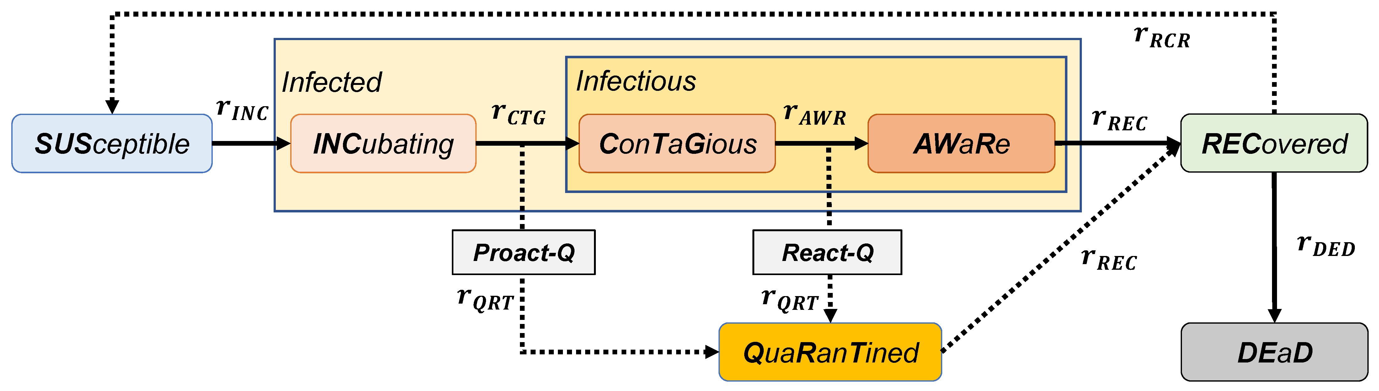
3.1. The SICARQD Epidemic Model

For the purpose of this study, we employ the complex epidemic model named SICARQD [22], summarized in Figure 3, and which defines the seven possible infectious states and particular transition rates. As such, an agent can be in one of the following states: susceptible SUS, incubating INC, contagious CTG, aware AWR, quarantined QRT, recovered REC, or dead DED. The transition from $SUS\to REC\to SUS$ is determined by several infection rates, the quarantine ratio, the quarantine policy, and the recurrence scenario. We summarize the main epidemic parameters as follows:

• $r_{INC}$: The rate of susceptible agents becoming infected in the vicinity of an infectious agent (which is in either of the two infectious states CTG or AWR). An agent in the $INC$ state will not infect other agents.
• $r_{CTG}$: The rate of incubating agents becoming contagious $CTG$ after a specific period (depending on the modeled virus). In this state, an agent does not know that it is infected (has no symptoms yet), but it infects others.
• $r_{AWR}$: The rate of contagious agents becoming aware after a specific period. In this state, an agent knows that it is infected (has symptoms) and infects other agents in its vicinity.
• $r_{REC}$: The rate of aware (or quarantined) agents recovering after an infectious period. The transition determines whether an agent has fully recovered, becoming temporarily immune ($REC$), or if the agent has died ($DED$) based on the death ratio $r_{DED}$. Recovered agents $REC$ may not be infected.
• $r_{RCR}$: The recurrence rate of recovered agents to become susceptible again after a specific period of recovery from infection.

In addition to the classical transition between susceptible, infected, and recovered states (SIR), SICARQD offers several transitions that increase the realism of epidemic modeling. First, a quarantine policy and a quarantine ratio $r_{QRT}$ will define when and how many agents transition to the $QRT$ state; in this state, agents are not be able to infect others and will transition directly to the $REC$ state (or, alternatively, to the $DED$ state). Second, our epidemic model adds a recurrence scenario, which determines whether or how fast agents transition back to $SUS$.

Since the epidemic model is not the main focus of this study, we briefly explain the quarantine and recurrence scenarios for agents. The quarantine policy is of three types:

• Proactive quarantine (proact-Q)—agents may be quarantined immediately as they become contagious $CTG$ and require real-time contact tracing and detection before symptoms appear).
• Reactive quarantine (react-Q)—agents may be quarantined as they become aware $AWR$, and require home isolation as symptoms appear.
• No quarantine (no-Q)—all infected agents remain active in the population.

In this study, we maintain the react-Q policy in most simulation scenarios, except when stated otherwise. We choose the reactive policy as the default because it is the most realistic in terms of large-scale real-world applicability when human and financial resources are limited, and quarantining is based largely on visible symptoms [28].

The recurrence scenario is of three types:

• Quick recurrence (quick-R)—short immunity duration of 3 months on average.
• Slow recurrence (slow-R)—longer immunity duration of 12 months on average.
• No recurrence (no-R)—meaning the rate $r_{RCR}=0$ and all recovered agents remain permanently immune.

In addition, in this study, we adopt the slow-R scenario in all cases since a `yearly’ recurrence is highly realistic for many ongoing/seasonal airborne viral infections (influenza [29] and COVID-19 [30]).

For additional details on the epidemic model, please refer to our previous study in [22].

3.2. Real-World Epidemic Parameters for SICARQD

The SICARQD allows customization for airborne infections, similar in complexity to influenza and coronaviruses. Therefore, given the ongoing relevance of the COVID-19 pandemic, in this study, we choose to parameterize our SICARQD model to the SARS-CoV-2 virus.

Table 1 details the values for each of the model’s parameters as found in the recent COVID-19 literature; we enumerate all the parameters illustrated in Figure 3, whose values are chosen based on an extensive literature review. In the situations where we find multiple parameter estimations, we choose either the worst case scenario (marked with ^**) or the average value (unmarked).

The impact of the last three parameters in Table 1 has been extensively studied in [22], being outside the scope of this paper. Relevant studies identify various recurrence rates for the SARS-CoV-2 virus, such as 3 months [31], 4–5 months [32], 6 months [33], and 1 year [34]. In this study, we adopt a slow-R scenario which translates to a fixed recurrence rate $r_{RCR}$ that causes agents to relapse back to $SUS$, on average, in 12 months’ simulation time. In terms of quarantine policy, we adopt a react-Q policy which means that agents may be quarantined—with a rate $r_{QRT}$—only once after in the $AWR$ state, when symptoms become visible. For all experiments, except one scenario, we assign the quarantine ratio to a fixed value.

Table 1. Parameterization of the SICARQD epidemic model detailing the values reported in the literature, the values selected in our model, and the relevant references. ** Assumed worst-case scenario based on the literature.

Model Parameter	Symbol	Literature Values	Assumed Value	References
Incubation rate	$r_{INC}$	0–5%	5% **	[26,35]
Incubation period	$r_{CTG}$	3–7 days	5 days	[36,37,38]
Contagion to symptoms onset	$r_{AWR}$	4–7 days	5.5 days	[35,36]
Symptoms onset to recovery	$r_{REC}$	10–14 days–6 w	14 days	[39,40,41]
Death ratio	$r_{DED}$	2–3.6%	3.6% **	[39,42]
Quarantine policy	$Q_{policy}$	various	react/proact-Q	[22,28]
Quarantine ratio	$r_{QRT}$	unknown	0–1	[22]
Recurrence scenario/rate	$r_{RCR}$	3–12 months	12 months	[31,34]

Table 1. Parameterization of the SICARQD epidemic model detailing the values reported in the literature, the values selected in our model, and the relevant references. ** Assumed worst-case scenario based on the literature.

Model Parameter	Symbol	Literature Values	Assumed Value	References
Incubation rate	$r_{INC}$	0–5%	5% **	[26,35]
Incubation period	$r_{CTG}$	3–7 days	5 days	[36,37,38]
Contagion to symptoms onset	$r_{AWR}$	4–7 days	5.5 days	[35,36]
Symptoms onset to recovery	$r_{REC}$	10–14 days–6 w	14 days	[39,40,41]
Death ratio	$r_{DED}$	2–3.6%	3.6% **	[39,42]
Quarantine policy	$Q_{policy}$	various	react/proact-Q	[22,28]
Quarantine ratio	$r_{QRT}$	unknown	0–1	[22]
Recurrence scenario/rate	$r_{RCR}$	3–12 months	12 months	[31,34]

All epidemic parameters are kept fixed (except for the $Q_{policy}$ in one simulation scenario) because the focus of this study is not to analyze the SICARQD model but rather to explore the realism and effectiveness of our urban spatial ABM. We note that in order to adjust the SICARQD model to another virus, it suffices to redefine the seven ratios in Table 1 according to the available epidemiological data.

3.3. Experimental Setup

In

Table 2. Input (upper panel) and output (lower panel) parameters for the ABM-SICARQD experimental setup, alongside the model symbols, default value in the model, and range of investigated values through simulation.

Model Parameter	Symbol	Default	Range
Agent population	A	1000	100–10,000 agents
Urban (total) POIs	P	100	1–1000 POIs
Agent POIs	$N_p$	10	1–50 POIs
Max. travel distance	$T_d$	500	100–1000
Quarantine ratio	$r_{QRT}$	0.5	0–1
Peak infection ratio	$\rho$	output	0–1
Total cases ratio	$\tau$	output	0...>1

, we enumerate the input and output parameters which are investigated during the simulation phase. The focus of this paper is to understand the influence of all the ABM parameters on the dynamics of an epidemic outbreak. Note that in order to reduce the complexity of the experiments, some of the parameters are kept fixed at all times, such as the urban area size $S=1000\times 1000$, the number of infectious seeds $N_s=1\%A$, the agent movement speed $A_v=2$, and the interaction radius with POIs ${\delta }_{interact}=4·A_v=8$.

We define the peak infection ratio $0\le \rho \le 1$ as the maximum number of daily cases, and it is expressed as a ratio of the total population A. To obtain $\rho$, we measure $\rho \left(t\right)$ at every time step t and keep the maximal value

$$\begin{array}{c}\hfill \rho \left(t\right)={\displaystyle \frac{Infected\left(t\right)}{A}}={\displaystyle \frac{INC\left(t\right)+CTG\left(t\right)+AWR\left(t\right)+QRT\left(t\right)}{A}}\\ \hfill \rho =max\left\{\rho \right(t\left)\right\}\end{array}$$

(7)

While $\rho$ quantifies the magnitude of the epidemic, we also measure the total number of cases $\tau$, for all simulation times, to obtain a perspective on the ratio between the peak and the duration of an outbreak. We define the ratio $\tau$ as the total number of susceptible $SUS$ agents who become incubating $INC$ over all agents in the population:

$$\tau ={\displaystyle \frac{{\sum }_t\left\{newcases\right\}}{A}}={\displaystyle \frac{{\sum }_t\left\{a_i\right|state\left(a_i\left(t\right)\right)=INC\&state\left(a_i(t-1)\right)=SUS\}}{A}}$$

(8)

In some cases where high population mixing allows for rapid contagion, the total cases ratio $\tau$ may be greater than 1; this means that agents are, on average, infected more than once during the simulation.

Figure 4 summarizes the ABM and SICARQD model input parameters, the agent setup phase, and the simulation steps with the end condition.

4. Simulation Results

In this section, we present the simulation results according to the experimental flow described in Figure 4 using the variable ABM input parameters from Table 2 and the epidemic parameters from Table 1. To this end, we investigate 6 values for the agent population $A\in \{100,\dots 10,000\}$, 6 values for the number of urban POIs $P\in \{1\dots 1000\}$, 6 values for the number of agent POIs $N_p\in \{1\dots 50\}$, 6 values of maximum travel distances $T_d\in \{100\dots 1000\}$, and 11 values for the quarantine ratio $r_{QRT}\in \{0,0.1\dots 1\}$. The pairs of simulations are $(A,P,r_{QRT}=0.5)$, $(A,N_p,r_{QRT}=0.5)$, $(A,r_{QRT})$, $(A,T_d,r_{QRT}=0.5)$, leading to 174 different scenarios. Each scenario is repeated 100 times and averaged, resulting in 17,400 simulations.

Since the number of numerical results is very high, we summarize all experiments by presenting only the peak infection ratio $\rho$ and the total cases ratio $\tau$ using intuitive plots instead of long tables. An example simulation using our SICARQD epidemic model, with slow-R and a quarantine ratio of $r_{QRT}=0.2$, is depicted in Figure 5.

The specific SICARQD infection recurrence is visible in Figure 5a as the number of susceptible $SUS$ agents increases slowly in time after the initial infection wave; similarly, the number of recovered $REC$ agents decreases after having reached a maximum right after the first wave. Furthermore, the three SICARQD specific infectious states and the quarantine state are visible in Figure 5b. Here, the total number of infected agents (red line) is the sum of all agents in either infected state, including $QRT$. The peak infection ratio $\rho$ is the maximum number of infected, namely, the peak of the infection wave; if more waves follow in time, then $\rho$ could be updated with a higher value. The three states $INC$, $CTG$, and $AWR$ follow quickly one after another as suggested by the vertical dotted lines through the peaks of each wave. Agents in the $QRT$ state become visible at the same time with $AWR$ because, due to the react-Q policy, an agent may only be quarantined after reaching the $AWR$ state and not sooner. Finally, the relatively small quarantine ratio $r_{QRT}=0.2$ determines the ratio between $AWR/QRT=(1-r_{QRT})/r_{QRT}=0.8/0.2=4$.

We start by measuring the two output epidemic measures defined in Table 2, namely, the peak infection ratio $\rho$ and the total cases ratio $\tau$ for an increasing agent population A. To put the results into perspective, Figure 6 plots the epidemic measures for different number of urban POIs P. In Figure 6a, we notice a linear increase from $\rho \approx$ 0–0.6 as the population increases, and are able to differentiate the impact of the total urban POIs P. Namely, for very few POIs P = 1–25 the epidemic reaches a higher peak sooner. As the population (density) increases, the results pinpoint towards a strong initial wave (i.e., a peak of $\rho$ = 0.5–0.6). In Figure 6b, we observe an accelerated increase in $\tau$ up to A = 500–1000, then a slower increase towards 100% of the population becoming infected. In the case of very few POIs, we report more than one new case per person on average due to the slow recurrence scenario.

In Figure 7, we highlight the importance of POIs in the urban area. Namely, both $\rho$ and $\tau$ drop abruptly as the number of urban POIs increases from P = 1–100 and then remain approximately constant regardless of the fact the P increases up to 1000 POIs. The initial drops are plotted in Figure 7a as percentages, and increase in magnitude, from 6% to 65%, as the population A decreases. This means that for a larger population density, the number of POIs is less impactful on the epidemic intensity. Here, we highlight the results only for a maximum population up to $A=2500$ (instead of A = 10,000) because the differences above $A=2500$ are insignificant in this plot. In panel Figure 7b, the total cases ratio $\tau$ follows a very similar trajectory. We note that for $P=1000$ POIs, the larger population results in $\times 21$ more cases than the lowest population.

Next, we provide a summary of how the epidemic measures are impacted by the maximum travel distance $T_d$. In Figure 8, we express the distance traveled $T_d\%S$ relative to the area S (in our case width $w=$ height h). The results prove that $T_d$ has a significant impact on the increase in both $\rho$ and $\tau$. In Figure 8a, the increase in $\rho$ starts with $T_d=200$, or $T_d\%S=0.2$ for the larger population densities, and with 0.4 for the smaller ones. Afterwards, the increase in the peak infection ratio remains linear up to $T_d\%S=1$. In Figure 8b, the increase in $\tau$ is more specific, with an accelerated increase between $T_d\%S$ = 0.2–0.4 followed by a stabilization around $\tau$ = 0.8–1 for higher values of $T_d$.

We further analyze how the number of agent POIs $N_p$ influences the epidemic outbreak measures (Figure 9). To this end, we find a significant increase in both epidemic measures but especially in the peak $\rho$ as the number of POIs increases from $N_p$ = 1–5. The results in Figure 9 can be corroborated by the results in Figure 7, where the epidemic intensity correlates with how well the population is distributed in multiple POIs. Here, when agents have a single POI on their path, the population mixing is highly reduced compared to when agents have five or more POIs to travel to. The increases in $\rho$ as $N_p$ increases are depicted in Figure 9a and range from 157% to 165% (depending on A). The total cases ratio $\tau$ also increases rapidly with the number of agent POIs, as shown in Figure 9b, and ranges from 97% to 105%.

Since we use the react-Q quarantine policy and the slow-R recurrence scenario in all presented results so far, we further explain the impact of the $Q_{policy}$ and the quarantine rate $r_{QRT}$ on the experimental setup. Figure 10 compares the epidemic dynamics from the perspective of react-Q and proact-Q policies. In Figure 10a, we show the drop in $\rho$ as the quarantine ratio increases and highlight the area $r_{QRT}$ = 0.6–1, where a rapid drop is noticeable. The measured drop in $\rho$ is more significant for a higher population (53%) than for a smaller population (8%).

In Figure 10b, the proact-Q underlines the importance of early quarantine, as the peak infection ratio drops sooner and more abruptly than for react-Q. We measure drops in $\rho$ of 79–92% for all populations starting with $r_{QRT}=0.4$. Nevertheless, while proact-Q is a more effective epidemic control policy, the real-world effort and costs are much higher than for adopting react-Q. For a full analysis aimed at the impact of patient quarantine and recurrence, please consult our previous study [22].

Please note that we do not plot the 95% CI for Figure 6, Figure 7, Figure 8, Figure 9 and Figure 10 (or similar statistic) in the results section because it would overload the already detailed plots, and make near lines hard to discern. Nevertheless, all results in Figure 6, Figure 7, Figure 8, Figure 9 and Figure 10 present the averages over 100 repeated simulations.

5. Discussion and Conclusions

Agent-based modeling is a powerful tool in computational epidemics for monitoring and managing infectious outbreaks. Unlike similar approaches, such as compartmental models or complex network-based approaches, ABMs can take into account the stochastic nature of human behavior and mobility, producing highly realistic computer-based simulations in dense urban environments [12,13,14,43].

Classic analytical modeling approaches employed in epidemics [5,44,45] include a time-dependent transmission rate to model changes in the infection rate caused by viral strain evolution, seasonality, social interactions, or governmental policies. By contrast to the differential equations of the compartmental models applied on the recent COVID-19 pandemic [5,44,45], ABMs study models of global mobility mechanisms based on emergent transmission dynamics. In this study, instead of a variable transmission rate, we use simulation on the ABM, resulting in a complex emergent population mixing instead of the compartmental models based on random uniform contact networks that are typically used to study epidemics spreading. Thus, modeling and quantifying human mobility is critical for studying the large-scale spatial transmission of infectious diseases [11,13,14].

In this study, we introduce a novel urban spatial agent-based model (ABM) based on the idea that urban points-of-interest (POIs) are hotspots for agent interaction (e.g., transmission of infection, opinion, and innovation) [19,20,21]. Therefore, we implement an agent’s travel routine as an independent random path from its home location through a number of $N_p$ POIs and back home. To this end, we only verify interaction within POIs and are able to reduce computational complexity considerably, from $O\left(A^2\right)$ to approximately $O(AP+0.0036A^2)\approx O\left(AP\right)$.

In addition, we incorporate the SICARQD epidemic model [22] to reproduce, analyze, and explain the parameters that affect the dynamics of an infectious outbreak in an urban setting. To showcase the efficiency of our ABM, we employ numerical simulation to measure the influence of urban-demographic parameters on the epidemic spreading based on complex and realistic agent mobility patterns.

We find that the agent population A (also interpreted as the population density given the fixed area $S=1000\times 1000\left[m\right]$) plays a crucial role in the development of an outbreak. Both the peak infection ratio $\rho$ and the total cases ratio $\tau$ increase linearly with A. Moreover, the number of total cases increases more rapidly up to A = 500–1000 then converges linearly towards $\tau \to 1$. If we relate to the real-world context, most metropolises have population densities between 4500 and 8000 inhabitants per km² [46]. By correlation, the density in our ABM is $A/S^2=A/(1000\left[m\right]x\times 1000\left[m\right])=A[/$km²]. Therefore, for large and dense cities, we notice that the impact of the number of urban POIs P is less important than the population A (see Figure 6).

A city having a very small number of urban POIs ($P\le 25$) can considerably increase the infection ratio (by 5–65%) as supported by the results in Figure 7. Nevertheless, most real-world mid- to large-size cities will have hundreds of POIs [19,20] so that the population concentration is more evenly distributed.

The maximum travel distance $T_d$ determines a delayed linear increase of the infection ratio, as shown in Figure 8. For very reduced mobility ($T_d<0.2$ of the available city area), the outbreak is mostly inhibited; as the permitted travel distance increases to $T_d$ = 0.2–0.4, we notice a rapid increase in the outbreak, proportional to the agent population A. Moreover, the total cases ratio $\tau$ presents a phase transition increase between $T_d$ = 0.2–0.6, earlier for the larger populations and later for the smaller ones.

The number of agent POIs $N_p$ are used to describe the number and diversity of the agent’s path. In this sense, we find that if agents are restricted to only one POI (except their home location), the outbreak is significantly reduced, compared to when agents may travel to $N_p\ge 5$ POIs (see Figure 9). We believe that more agent POIs translate to proportionally higher population mixing, which, in turn, increases the infection ratio. The increases in the peak infection ratio $\rho$, when increasing $N_p$ from 1 to 5, are between 149 and 165%; for the total cases ratio $\tau$, the increases are ≈$100\%$ (i.e., double the number of infections).

Our last analyzed scenario is supported by the mechanics of the SICARQD epidemic model, namely, a comparison between the impact of a reactive (react-Q) and a proactive (proact-Q) quarantine policy. In this sense, Figure 10 pinpoints that late quarantine react-Q (i.e., based on quarantining patients after they become aware of their symptoms) is much less effective than early quarantine proact-Q (i.e., based on quarantining patients preemptively, using contact tracing, and before their symptoms may appear). For react-Q, we measure a slow drop in the infection ratio, more pronounced between $r_{QRT}$ = 0.6–1, of 8–53%. Conversely, for proact-Q, we measure an abrupt drop in the infection ratio between $r_{QRT}$ = 0.4–0.8 of 79–92%. Thus, proact-Q can be 1.7–10× more effective (depending on population density) in reducing the peak infection ratio $\rho$. Nevertheless, the proact-Q scenario, with a high quarantine ratio, is very difficult to implement in a real context due to the high resource cost.

Overall, we summarize the findings validated through the usage of our urban spatial ABM and the SICARQD epidemic model as follows.

Urban/policy factors which increase the peak infection ratio $\rho$ and the total cases ratio $\tau$:

• Agent population (A)/density ($A/S$)—linear increase.
• Maximum permitted travel distance for agents ($T_d$)—linear increase but only above $T_d>0.2\%S$.
• Number of agent POIs ($N_p$)—logarithmic increase for $N_p$ = 1–5, then negligible increase after $N_p>5$.

Urban/policy factors which decrease the peak infection ratio $\rho$ and the total cases ratio $\tau$:

• Number of urban POIs (P)—logarithmic decrease for P = 1–100, then negligible decrease after $P\ge 100$.
• Ratio of quarantined infected individuals ($r_{QRT}$)—logarithmic decrease, pronounced after $r_{QRT}>0.4$.

Additionally, the nature of the virus will determine the immunization period, modeled as the recurrence scenario in our SICARQD model. A quick-R scenario will increase the infected ratio in time compared to a no-R or slow-R scenario. Also, a proactive quarantine policy will significantly decrease the infection count compared to a reactive policy, for quarantine ratios of $r_{QRT}>0.4$, by 1.7–10×, depending on the agent density.

Compared to other classic ABM approaches, such as [11,12], which do not employ POIs, our study is able to point out two important aspects of infectious dynamics:

• The epidemic recurrence phenomenon is induced by the emergent agent mobility modeled in our system. More specifically, recovered agents lose their immunity in time (based on either slow-R or quick-R) and may travel to infected POIs again, and thus, infectious hotspots will be maintained for a very long duration, replicating the residual waves seen after the COVID-19 pandemic started.
• The proactive quarantine (proact-Q) in correlation to a higher quarantine ratio ($r_{QRT}$) triggers a phase transition, reducing the total infected population by over 90% (Figure 10b) compared to the reactive quarantine (Figure 10a). Therefore, a proactive quarantine associated with a strict quarantine ratio can almost completely inhibit infectious spread.

Several limitations of this study are enumerated below. First, the agent model presented is confined to a closed area $S=w·h$ in order to replicate an urban setting. However, we plan to extend the ABM so that it can represent multiple independent cities, by running parallel simulations, or interdependent cities, by allowing a fraction of agents to travel between cities [47]. Second, all POIs are considered equal and are placed equidistant. The present agent redirection algorithm can use any mapping of POIs, so one can initialize POIs using any spatial distribution. In terms of equal POIs, our model can be augmented by defining specific classes of POIs, with their own maximum occupancy and time spent per agent. Third, we consider all agents identical: they have the same speed, the same number of POIs ($N_p$), and they do not belong to demographic groups (e.g., age and gender). However, our study maintains a generic focus on POIs rather than specific demographic aspects. Nevertheless, the ABM can be further improved to incorporate different individual traits, with different types of POI requirements.

An underestimated element in the adoption of quarantine policies during epidemics is the psychological human factor. We note as possible development directions in our methodology the consideration of the harmful mental effects caused by quarantine protocols [48], as well as the natural intervention fatigue of maintaining quarantine strictness over a longer period [49].

In addition to the scientific potential of our proposed general purpose, customizable, and computationally efficient ABM framework, our observations find immediate applicability in the ongoing COVID-19 pandemic, as well as foreseeable epidemics with similar airborne transmission. We validate our ABM in the context of epidemic outbreaks, but this model can be further adopted in social physics, or political and environmental sciences. For instance, our ABM can be used to analyze opinion injection strategies and competing influence dynamics [50,51,52], additional vaccination/immunization strategies for viral outbreaks [53,54], or political polarization and fake-news dynamics [55,56].

We believe that this study has great potential to have a consistent impact in the fields of computational epidemics, mathematical modeling, computer science, and public health by addressing major social and scientific challenges [2,3,57,58].

Future research directions may include (i) extending the ABM to a multi-urban model with interdependent cities, (ii) defining POI classes with unique characteristics and requirements, (iii) introducing multiple agent categories with unique mobility patterns and needs, and (iv) updating SICARQD to also model vaccination and tuning the epidemic parameters to custom regions and viruses of scientific interest.

References

1. Salathé, M.; Jones, J.H. Dynamics and control of diseases in networks with community structure. PLoS Comput. Biol. 2010, 6, e1000736. [Google Scholar] [CrossRef] [PubMed]
2. Keeling, M. The implications of network structure for epidemic dynamics. Theor. Popul. Biol. 2005, 67, 1–8. [Google Scholar] [CrossRef] [PubMed]
3. Keeling, M.J.; Rohani, P. Modeling Infectious Diseases in Humans and Animals; Princeton University Press: Princeton, NJ, USA, 2008. [Google Scholar]
4. Hellewell, J.; Abbott, S.; Gimma, A.; Bosse, N.I.; Jarvis, C.I.; Russell, T.W.; Munday, J.D.; Kucharski, A.J.; Edmunds, W.J.; Funk, S.; et al. Feasibility of controlling COVID-19 outbreaks by isolation of cases and contacts. Lancet Glob. Health 2020, 8, e488–e496. [Google Scholar] [CrossRef] [PubMed]
5. Kucharski, A.J.; Russell, T.W.; Diamond, C.; Liu, Y.; Edmunds, J.; Funk, S.; Eggo, R.M.; Centre for Mathematical Modelling of Infectious Diseases COVID-19 Working Group. Early dynamics of transmission and control of COVID-19: A mathematical modelling study. Lancet Infect. Dis. 2020, 20, 553–558. [Google Scholar]
6. Koo, J.R.; Cook, A.R.; Park, M.; Sun, Y.; Sun, H.; Lim, J.T. Interventions to mitigate early spread of COVID-19 in Singapore: A modelling study. Lancet Infect Dis. 2020, 20, 678–688. [Google Scholar] [CrossRef]
7. Cohen, J.; Kupferschmidt, K. Countries test tactics in ‘war’ against COVID-19. Science 2020, 367, 1287–1288. [Google Scholar] [CrossRef]
8. Ferguson, N.M.; Cummings, D.A.; Fraser, C.; Cajka, J.C.; Cooley, P.C.; Burke, D.S. Strategies for mitigating an influenza pandemic. Nature 2006, 442, 448–452. [Google Scholar] [CrossRef]
9. So, M.K.; Tiwari, A.; Chu, A.M.; Tsang, J.T.; Chan, J.N. Visualizing COVID-19 pandemic risk through network connectedness. Int. J. Infect. Dis. 2020, 96, 558–561. [Google Scholar] [CrossRef]
10. Silva, C.J.; Cantin, G.; Cruz, C.; Fonseca-Pinto, R.; Passadouro, R.; Dos Santos, E.S.; Torres, D.F. Complex network model for COVID-19: Human behavior, pseudo-periodic solutions and multiple epidemic waves. J. Math. Anal. Appl. 2022, 514, 125171. [Google Scholar] [CrossRef]
11. Hackl, J.; Dubernet, T. Epidemic spreading in urban areas using agent-based transportation models. Future Internet 2019, 11, 92. [Google Scholar] [CrossRef]
12. Nadini, M.; Zino, L.; Rizzo, A.; Porfiri, M. A multi-agent model to study epidemic spreading and vaccination strategies in an urban-like environment. Appl. Netw. Sci. 2020, 5, 68. [Google Scholar] [CrossRef] [PubMed]
13. De Oliveira, L.B.; Camponogara, E. Multi-agent model predictive control of signaling split in urban traffic networks. Transp. Res. Part C Emerg. Technol. 2010, 18, 120–139. [Google Scholar] [CrossRef]
14. Zhuge, C.; Shao, C.; Wei, B. An agent-based spatial urban social network generator: A case study of Beijing, China. J. Comput. Sci. 2018, 29, 46–58. [Google Scholar] [CrossRef]
15. Macal, C.M.; North, M.J. Agent-based modeling and simulation. In Proceedings of the 2009 Winter Simulation Conference (WSC), Austin, TX, USA, 13–16 December 2009; IEEE: Piscataway, NJ, USA, 2009; pp. 86–98. [Google Scholar]
16. Badr, H.S.; Du, H.; Marshall, M.; Dong, E.; Squire, M.M.; Gardner, L.M. Association between mobility patterns and COVID-19 transmission in the USA: A mathematical modelling study. Lancet Infect. Dis. 2020, 20, 1247–1254. [Google Scholar] [CrossRef] [PubMed]
17. Adam, D. Special report: The simulations driving the world’s response to COVID-19. Nature 2020, 580, 316–319. [Google Scholar] [CrossRef] [PubMed]
18. Hinch, R.; Probert, W.J.; Nurtay, A.; Kendall, M.; Wymant, C.; Hall, M.; Lythgoe, K.; Bulas Cruz, A.; Zhao, L.; Stewart, A.; et al. OpenABM-Covid19—An agent-based model for non-pharmaceutical interventions against COVID-19 including contact tracing. PLoS Comput. Biol. 2021, 17, e1009146. [Google Scholar] [CrossRef]
19. Chang, S.; Pierson, E.; Koh, P.W.; Gerardin, J.; Redbird, B.; Grusky, D.; Leskovec, J. Mobility network models of COVID-19 explain inequities and inform reopening. Nature 2021, 589, 82–87. [Google Scholar] [CrossRef]
20. Li, Q.; Bessell, L.; Xiao, X.; Fan, C.; Gao, X.; Mostafavi, A. Disparate patterns of movements and visits to points of interest located in urban hotspots across US metropolitan cities during COVID-19. R. Soc. Open Sci. 2021, 8, 201209. [Google Scholar] [CrossRef]
21. Nian, G.; Peng, B.; Sun, D.; Ma, W.; Peng, B.; Huang, T. Impact of COVID-19 on urban mobility during post-epidemic period in megacities: From the perspectives of taxi travel and social vitality. Sustainability 2020, 12, 7954. [Google Scholar] [CrossRef]
22. Topîrceanu, A. On the Impact of Quarantine Policies and Recurrence Rate in Epidemic Spreading Using a Spatial Agent-Based Model. Mathematics 2023, 11, 1336. [Google Scholar] [CrossRef]
23. Mao, L.; Bian, L. Spatial–temporal transmission of influenza and its health risks in an urbanized area. Comput. Environ. Urban Syst. 2010, 34, 204–215. [Google Scholar] [CrossRef] [PubMed]
24. Topirceanu, A.; Udrescu, M.; Marculescu, R. Centralized and decentralized isolation strategies and their impact on the COVID-19 pandemic dynamics. arXiv 2020, arXiv:2004.04222. [Google Scholar]
25. Newman, M.E. Spread of epidemic disease on networks. Phys. Rev. E 2002, 66, 016128. [Google Scholar] [CrossRef]
26. Pastor-Satorras, R.; Castellano, C.; Van Mieghem, P.; Vespignani, A. Epidemic processes in complex networks. Rev. Mod. Phys. 2015, 87, 925. [Google Scholar] [CrossRef]
27. Tako, A.A.; Robinson, S. Comparing discrete-event simulation and system dynamics: Users’ perceptions. In System Dynamics; Springer: Berlin/Heidelberg, Germany, 2018; pp. 261–299. [Google Scholar]
28. Peak, C.M.; Kahn, R.; Grad, Y.H.; Childs, L.M.; Li, R.; Lipsitch, M.; Buckee, C.O. Individual quarantine versus active monitoring of contacts for the mitigation of COVID-19: A modelling study. Lancet Infect. Dis. 2020, 20, 1025–1033. [Google Scholar] [CrossRef]
29. Dushoff, J.; Plotkin, J.B.; Levin, S.A.; Earn, D.J. Dynamical resonance can account for seasonality of influenza epidemics. Proc. Natl. Acad. Sci. USA 2004, 101, 16915–16916. [Google Scholar] [CrossRef]
30. Edridge, A.W.; Kaczorowska, J.; Hoste, A.C.; Bakker, M.; Klein, M.; Loens, K.; Jebbink, M.F.; Matser, A.; Kinsella, C.M.; Rueda, P.; et al. Seasonal coronavirus protective immunity is short-lasting. Nat. Med. 2020, 26, 1691–1693. [Google Scholar] [CrossRef]
31. Ward, H.; Cooke, G.; Atchison, C.J.; Whitaker, M.; Elliott, J.; Moshe, M.; Brown, J.C.; Flower, B.; Daunt, A.; Ainslie, K.E.; et al. Declining prevalence of antibody positivity to SARS-CoV-2: A community study of 365,000 adults. MedRxiv 2021. [Google Scholar] [CrossRef]
32. Gudbjartsson, D.F.; Norddahl, G.L.; Melsted, P.; Gunnarsdottir, K.; Holm, H.; Eythorsson, E.; Arnthorsson, A.O.; Helgason, D.; Bjarnadottir, K.; Ingvarsson, R.F.; et al. Humoral immune response to SARS-CoV-2 in Iceland. N. Engl. J. Med. 2020, 383, 1724–1734. [Google Scholar] [CrossRef]
33. Zuo, J.; Dowell, A.; Pearce, H.; Verma, K.; Long, H.; Begum, J.; Aiano, F.; Amin-Chowdhury, Z.; Hallis, B.; Stapley, L.; et al. Robust SARS-CoV-2-specific T-cell immunity is maintained at 6 months following primary infection. Nat. Immunol. 2020, 22, 620–626. [Google Scholar] [CrossRef]
34. Zayet, S.; Royer, P.Y.; Toko, L.; Pierron, A.; Gendrin, V.; Klopfenstein, T. Recurrence of COVID-19 after recovery? A case series in health care workers, France. Microbes Infect. 2021, 23, 104803. [Google Scholar] [CrossRef]
35. Jones, N.R.; Qureshi, Z.U.; Temple, R.J.; Larwood, J.P.; Greenhalgh, T.; Bourouiba, L. Two metres or one: What is the evidence for physical distancing in COVID-19? BMJ 2020, 370, m3223. [Google Scholar] [CrossRef] [PubMed]
36. Lauer, S.A.; Grantz, K.H.; Bi, Q.; Jones, F.K.; Zheng, Q.; Meredith, H.R.; Azman, A.S.; Reich, N.G.; Lessler, J. The incubation period of coronavirus disease 2019 (COVID-19) from publicly reported confirmed cases: Estimation and application. Ann. Intern. Med. 2020, 172, 577–582. [Google Scholar] [CrossRef] [PubMed]
37. Quesada, J.; López-Pineda, A.; Gil-Guillén, V.; Arriero-Marín, J.; Gutiérrez, F.; Carratala-Munuera, C. Incubation period of COVID-19: A systematic review and meta-analysis. Rev. Clin. Esp. (Engl. Ed.) 2021, 221, 109–117. [Google Scholar] [CrossRef] [PubMed]
38. Li, Q.; Guan, X.; Wu, P.; Wang, X.; Zhou, L.; Tong, Y.; Ren, R.; Leung, K.S.; Lau, E.H.; Wong, J.Y.; et al. Early transmission dynamics in Wuhan, China, of novel coronavirus–infected pneumonia. N. Engl. J. Med. 2020, 382, 1199–1207. [Google Scholar] [CrossRef] [PubMed]
39. Baud, D.; Qi, X.; Nielsen-Saines, K.; Musso, D.; Pomar, L.; Favre, G. Real estimates of mortality following COVID-19 infection. Lancet Infect. Dis. 2020, 20, 773. [Google Scholar] [CrossRef]
40. Eurosurveillance Editorial Team. Updated rapid risk assessment from ECDC on the novel coronavirus disease 2019 (COVID-19) pandemic: Increased transmission in the EU/EEA and the UK. Euro. Surveill. 2020, 25, 2003121. [Google Scholar]
41. Linton, N.M.; Kobayashi, T.; Yang, Y.; Hayashi, K.; Akhmetzhanov, A.R.; Jung, S.M.; Yuan, B.; Kinoshita, R.; Nishiura, H. Incubation period and other epidemiological characteristics of 2019 novel coronavirus infections with right truncation: A statistical analysis of publicly available case data. J. Clin. Med. 2020, 9, 538. [Google Scholar] [CrossRef]
42. Wang, C.; Horby, P.W.; Hayden, F.G.; Gao, G.F. A novel coronavirus outbreak of global health concern. Lancet 2020, 395, 470–473. [Google Scholar] [CrossRef]
43. Topirceanu, A.; Udrescu, M. Statistical fidelity: A tool to quantify the similarity between multi-variable entities with application in complex networks. Int. J. Comput. Math. 2017, 94, 1787–1805. [Google Scholar] [CrossRef]
44. Girardi, P.; Gaetan, C. An SEIR Model with Time-Varying Coefficients for Analyzing the SARS-CoV-2 Epidemic. Risk Anal. 2023, 43, 144–155. [Google Scholar] [CrossRef]
45. Yin, K.; Mondal, A.; Ndeffo-Mbah, M.; Banerjee, P.; Huang, Q.; Gurarie, D. Bayesian inference for COVID-19 transmission dynamics in India using a modified SEIR model. Mathematics 2022, 10, 4037. [Google Scholar] [CrossRef]
46. Rodrigue, J.P. The Geography of Transport Systems; Routledge: London, UK, 2020. [Google Scholar]
47. Topîrceanu, A.; Precup, R.E. A novel geo-hierarchical population mobility model for spatial spreading of resurgent epidemics. Sci. Rep. 2021, 11, 14341. [Google Scholar] [CrossRef] [PubMed]
48. Fontanari, J.F. A stochastic model for the influence of social distancing on loneliness. Phys. A Stat. Mech. Its Appl. 2021, 584, 126367. [Google Scholar] [CrossRef]
49. Rypdal, K.; Bianchi, F.M.; Rypdal, M. Intervention fatigue is the primary cause of strong secondary waves in the COVID-19 pandemic. Int. J. Environ. Res. Public Health 2020, 17, 9592. [Google Scholar] [CrossRef]
50. Topîrceanu, A. Benchmarking Cost-Effective Opinion Injection Strategies in Complex Networks. Mathematics 2022, 10, 2067. [Google Scholar] [CrossRef]
51. Li, W.; Xue, X.; Pan, L.; Lin, T.; Wang, W. Competing spreading dynamics in simplicial complex. Appl. Math. Comput. 2022, 412, 126595. [Google Scholar] [CrossRef]
52. Topîrceanu, A. Competition-Based Benchmarking of Influence Ranking Methods in Social Networks. Complexity 2018, 2018. [Google Scholar] [CrossRef]
53. Pastor-Satorras, R.; Vespignani, A. Immunization of complex networks. Phys. Rev. E 2002, 65, 036104. [Google Scholar] [CrossRef]
54. Topîrceanu, A. Immunization using a heterogeneous geo-spatial population model: A qualitative perspective on COVID-19 vaccination strategies. Procedia Comput. Sci. 2021, 192, 2095–2104. [Google Scholar] [CrossRef]
55. Wojcieszak, M.; Sobkowicz, P.; Yu, X.; Bulat, B. What information drives political polarization? Comparing the effects of in-group praise, out-group derogation, and evidence-based communications on polarization. Int. J. Press/Politics 2022, 27, 325–352. [Google Scholar] [CrossRef]
56. Bovet, A.; Makse, H.A. Influence of fake news in Twitter during the 2016 US presidential election. Nat. Commun. 2019, 10, 7. [Google Scholar] [CrossRef] [PubMed]
57. Topîrceanu, A.; Udrescu, M.; Udrescu, L.; Ardelean, C.; Dan, R.; Reisz, D.; Mihaicuta, S. SAS score: Targeting high-specificity for efficient population-wide monitoring of obstructive sleep apnea. PLoS ONE 2018, 13, e0202042. [Google Scholar] [CrossRef]
58. Udrescu, L.; Bogdan, P.; Chiş, A.; Sîrbu, I.O.; Topîrceanu, A.; Văruţ, R.M.; Udrescu, M. Uncovering New Drug Properties in Target-Based Drug–Drug Similarity Networks. Pharmaceutics 2020, 12, 879. [Google Scholar] [CrossRef] [PubMed]
Figure 1. Schematic representation of the main defining properties of the urban ABM. (a) A rectangular (or square) space S is defined by width and height ( S = w · h ), which is divided as a matrix of uniform square areas based on the fixed distance P d between POIs. An urban POI is placed in each intersection of the dotted lines, including along the margins of the area, e.g., 7 × 7 POIs are placed in the example model. The orange icons suggest possible urban POIs, such as shops, offices, train stations, churches, hospitals, etc. (b) For each agent (green dot), a number of N p POIs are assigned within the maximum travel distance T d . Each randomly placed POI (gray dot) is assigned as the nearest urban POI (orange dot) within the permitted gray square area. (c) An agent (green dot) will travel, independently of any other agent, along the designated green path through each POI (orange dots) and return to its home position; then, after a timeout, the process of visiting the same list of POIs repeats. Other agents (blue dot) have different paths to follow. The (infectious) interaction is only possible if two agents are at the same simulation time t at the same POI.
Mathematics 12 02765 g001
Figure 2. Overview of the agent movement characteristics. (a) An agent (green dot) moves in a straight line towards the next POI (orange dots), or returns home, with a constant speed of A v . Given the 2D space, two components of the speed are calculated, v x , v y , based on the ratio between the horizontal and vertical distances, d x , d y , towards the next POI; this ratio determines the direction of movement. The sum of the two squared speeds equals the square of the agent speed A v ; thus, all agents move at the same speed, regardless of their direction. (b) Three agents (green, yellow, and blue) move towards the central POI (orange). The state of being inside a POI translates to being within δ i n t e r a c t / 2 = 2 · A v of the POI itself. Once an agent enters the target area (gray square), a new destination is immediately computed, and the agent changes its direction. In the example, all three agents move iteratively with speed A v towards the POI, step by step, as suggested by the short arrows and time steps ( t k ). Agents a 1 and a 2 enter the POI at time t k + 3 and exit immediately at t k + 4 ; agent a 3 enters the POI at t k + 1 , changes course, and exits at t k + 4 . In this sense, all three agents interact with each other only for one iteration ( t k + 3 ), whereas agent a 3 may interact with other agents for three iterations as shown in the upper right panel.
Mathematics 12 02765 g002
Figure 3. Schematic of the SICARQD epidemic model with its seven states and transmission dynamics based on the infection ratios. The characteristic two-stage infectious process ( C T G and A W R ) enables our model to differentiate between and early (proact-Q) and a late (react-Q) quarantine policies. The ratio r Q R T of agents moved to quarantine Q R T will no longer infect other agents and will transit directly to the recovered R E C or dead D E D states. Moreover, recovered R E C agents may become susceptible S U S again, in time, based on the imposed recurrence scenario.
Mathematics 12 02765 g003
Figure 4. Flow diagram of the experimental setup, from Start to End. The specific input parameters are fixed for the urban area, the ABM, and the epidemic model. Next, the ABM is created by designating the urban POIs inside the area S, placing all A agents and assigning their own POIs to visit within the distance T d ; also, all agents are set as susceptible, except a number of N s agents who are infected to trigger the epidemic outbreak. The simulation phase (gray area) consists of three repeated steps: updating the epidemic state of each agent, updating the position of each agent, and checking the agent interaction (whether inside POI, and transmitting infection to other agents). The process repeats as long as the simulation time t S I M _ T I M E .
Mathematics 12 02765 g004
Figure 5. The dynamics of an epidemic outbreak using the SICARQD model with slow infection recurrence (slow-R) and a reactive quarantine policy (react-Q). (a) The total cases ratio τ increases steadily and becomes > 1 , meaning that agents become infected more than once, on average; the similar drop in R E C and increase in S U S is caused by the recurrent infection scenario. (b) Detail of the dynamics of the infected states, highlighting the maximum of the total infected as the peak infection rate ρ . A quarantine ratio of r Q R T = 0.2 is used, which means that 20% of agents who become A W R will be quarantined (i.e., the ratio A W R / Q R T = 4 ).
Mathematics 12 02765 g005
Figure 6. Impact of the agent population A in terms of (a) peak infection ratio ρ and (b) total cases ratio τ for different values of number of urban POIs P. In several points, we highlight the percentage difference (%) between the highest and lowest ρ . Both plotted epidemic measures show particular linear increases. The highest infection rate is achieved for one single POI per system (blue line), suggesting that very high population concentration favors faster epidemic spreading.
Mathematics 12 02765 g006
Figure 7. Impact of the number of urban POIs P on the (a) peak infection ratio ρ and the (b) total cases ratio τ , for increasing population sizes A = 100 2500 . The drops from P = 1 to P = 100 are expressed as percentages from the maximum value ρ .
Mathematics 12 02765 g007
Figure 8. Impact of the maximum travel distance T d (expressed relative to the urban area size S) on the (a) peak infection ratio ρ and the (b) total cases ratio τ , for different population sizes A. Both epidemic measures increase linearly after T d 0.2 (for larger populations), or after T d 0.4 (for smaller populations). The highest differences in terms of epidemic measures are calculated around T d = 0.4 , where higher populations achieve an ≈×4–5 higher infection count.
Mathematics 12 02765 g008
Figure 9. Impact of the number of agent POIs N p of each agent T d on the (a) peak infection ratio ρ and the (b) total cases ratio τ , for different population sizes A. In both panels, we notice a rapid increase from N p = 1 to N p = 5 , which translates to an agent visiting more than one place on its travel routine, thus rapidly increasing the population mixing. The peak infection ratio ρ increases by over 150% from the initial increase in N p , while the total cases ratio τ increases by ≈ 100 % .
Mathematics 12 02765 g009
Figure 10. Impact of the (a) proactive and (b) reactive quarantine policies given an increasing quarantine ratio r Q R T on the agent populations A. The red vertical bars delimit a visible phase transition area between r Q R T = 0.6–1 (react-Q), respectively r Q R T = 0.4–0.8 (proact-Q). The percentages in each panel represent relative decreases in r Q R T between the vertical bars. The decrease in peak infection ratio ρ is significantly more abrupt, as r Q R T increases, for the proact-Q policy (79–92%).
Mathematics 12 02765 g010