Abstract
The task of finding natural groupings within a dataset exploiting proximity of samples is known as clustering, an unsupervised learning approach. Density-based clustering algorithms, which identify arbitrarily shaped clusters using spatial dimensions and neighbourhood aspects, are sensitive to the selection of parameters. For instance, DENsity CLUstEring (DENCLUE)—a density-based clustering algorithm—requires a trial-and-error approach to find suitable parameters for optimal clusters. Earlier attempts to automate the parameter estimation of DENCLUE have been highly dependent either on the choice of prior data distribution (which could vary across datasets) or by fixing one parameter (which might not be optimal) and learning other parameters. This article addresses this challenge by learning the parameters of DENCLUE through the differential evolution optimisation technique without prior data distribution assumptions. Experimental evaluation of the proposed approach demonstrated consistent performance across datasets (synthetic and real datasets) containing clusters of arbitrary shapes. The clustering performance was evaluated using clustering validation metrics (e.g., Silhouette Score, Davies–Bouldin Index and Adjusted Rand Index) as well as qualitative visual analysis when compared with other density-based clustering algorithms, such as DPC, which is based on weighted local density sequences and nearest neighbour assignments (DPCSA) and Variable KDE-based DENCLUE (VDENCLUE).
Keywords:
DENCLUE algorithm; differential evolution; density-based clustering; parameter optimisation; cluster validation metrics; cluster coverage optimisation; unsupervised learning MSC:
68W50
1. Introduction
Clustering, a fundamental and unsupervised technique in data analysis and machine learning, identifies and groups similar data points based on their inherent characteristics. With applications in various fields, such as market segmentation, image and pattern recognition and biological data analysis, clustering enables the discovery of natural groupings within complex datasets. Commonly used clustering algorithms include partition-based, hierarchical, model-based, grid-based and density-based methods, each utilising different criteria for similarity measurement and clustering evaluation [,,]. Each has its strengths and limitations, but density-based clustering methods, such as DBSCAN and DENCLUE, have proven effective in identifying clusters of arbitrary shapes and managing noise [,].
Density-based clustering algorithms typically work by separating high-density regions from low-density areas to form clusters. Using spatial features allows density-based algorithms to handle better complex data structures with clusters of varying densities, shapes and sizes. Density-Based Spatial Clustering of Applications with Noise (DBSCAN) [] and DENsity CLUstEring (DENCLUE) [] are two well-known density-based clustering algorithms that can identify clusters of arbitrary shapes and effectively handle noise. Other density-based methods include OPTICS [], SNN [], DbKmeans [], SPARCL [], CLASP [], GDBSCAN [] and MAP-DP [], with some modern density algorithms focusing on density peak clustering, such as DPCSA []. Besides strengths, each method has its limitations, such as high computational complexity, assumption of convex-shaped clusters, high sensitivity to noise and challenges with high-dimensional datasets []. Additionally, most of these methods are sensitive to the user-defined or heuristic-based input parameters, limiting their applicability. DENCLUE, while excelling in identifying clusters of arbitrary shapes and densities, handling noise well and being suitable for high-dimensional datasets [], still suffers from sensitivity to input parameters [], which are user-defined and selected through trial-and-error [,]. Although there have been advancements in methods for estimating DENCLUE’s parameters from datasets, there are notable deficiencies. Some common issues are dependency on the manual adjustment of heuristics, challenges in consistently yielding optimised clustering outcomes for diverse data structures and difficulties in effectively handling varying densities and inherent noise. Additionally, these methods have higher computational requirements, reliance on specific dataset properties and significant domain knowledge requirements.
With ongoing advancements in parameter optimisation techniques, it is becoming evident that methods like Differential Evolution (DE) have great potential. DE is a widely used population-based metaheuristic optimisation technique, well-known for its ability to optimise complex functions, and can be utilised for parameter optimisation in density-based clustering methods like DENCLUE. It is easy to implement and outperforms other methods within the same category [,,] in various situations, including unimodal and multimodal ones. Given DE’s significant efficacy, resilience and capacity to handle complex parameter spaces, its use can lead to more precise and adaptive parameter estimations. Hence, it is hypothesised that DE can address DENCLUE’s sensitivity to parameter values. This study aims to enhance the parameter estimation process for DENCLUE through Differential Evolution. The method’s performance will be assessed on various real and synthetic datasets containing clusters of diverse shapes, sizes and densities.
The rest of the article is organised as follows: Section 2 presents a background to DENCLUE, DE and parameter estimation. Section 3 presents the detailed workings of the proposed DE-based DENCLUE parameter optimisation technique. Section 4 details the complete setup for the experiments performed. Section 5 explains the results and discusses the insights gained and their implications. Section 6 concludes the article.
2. Background
2.1. DENCLUE Algorithm
DENCLUE is a density-based clustering method developed by Hinneburg and Keim []. It is an efficient density-based clustering algorithm that models the density of a data point as the sum of influence functions from all other points, identifying clusters by locating density attractors or local maxima. The influence function can be defined by a distance function (such as Euclidean) that determines the distance between two data points. An example of influence function that uses a Gaussian kernel is given in Equation (1), where the d is the distance function, x and y are two data points and the parameter σ is the bandwidth/influence range of the kernel.
The density of a data point is computed by a density function shown in Equation (2), where is the data point for which density is being computed, ’s are the other data points.
A hill climbing algorithm finds the local maximum (also known as a density attractor) of the density function for a data point. The density attractors with densities less than the threshold ξ are discarded, and a data point with a density attractor that is insignificant is considered as noise.
DENCLUE is suitable for high-dimensional datasets with noise and complex data structures with clusters of varying shapes, sizes and densities. DENCLUE, besides its strengths, has limitations: (1) it used as a trial-and-error approach for initial parameters; (2) it uses single global cluster density parameters, ignoring the variation across cluster sizes; and (3) it uses a fixed step size in the hill-climbing while finding density attractors, resulting in lower convergence [].
The recent innovations in DENCLUE parameter estimation, summarised in Table 1, come with their strengths and limitations. For instance, the KNN–DENCLUE method [] combines K nearest neighbours with DENCLUE to estimate parameters, but it introduces additional user-defined parameters and requires visual analysis to set the minimum density threshold. Similarly, methods introduced by Luo et al. [] and Zhang et al. [] have improved speed and noise detection but depend on assumptions about cluster numbers and still require user input for critical parameters like the influence range. Other approaches, such as the Bayesian method [] and the Cauchy optimisation gradient technique in HD–DENCLUE [], offer improved parameter estimation methods. However, these methods either remain works-in-progress or still require user-defined noise thresholds. VDENCLUE [] and DE-based approaches [] enhance adaptability and execution time but lack detailed methodology, experiments over diverse datasets and are still sensitive to user-defined parameters. DENCLUE 2.0 [] introduced a new hill-climbing method that adjusts the step size automatically, which has improved speed, but still requires an influence range parameter and assumes a Gaussian kernel.

Table 1.
Parameter Estimation Methods in DENCLUE.
While existing methods present notable limitations, there is a compelling need for a fully automated parameter estimation method for DENCLUE that assumes no prior dataset distribution, does not depend on dataset-specific heuristics and requires no domain knowledge or user input.
2.2. Differential Evolution
Differential Evolution (DE) is a population-based metaheuristic technique [] for solving optimisation problems in continuous spaces. DE has two main phases: (1) initialisation of the population; and (2) population evolution. In the initialisation phase, a uniformly distributed random population is generated by Equation (3), where POP represents the population, G is the current generation and NP is the size of the population in terms of the number of solutions. Each is an individual solution in the population and is represented by a D-dimensional vector of continuous values . The dimensions (D) of the vector are also called the parameters of the vector.
In the evolution phase, the mutation, crossover and selection are performed iteratively. A mutant vector is generated for each solution taken from the population, known as the target vector. A typical mutation operation is shown in Equation (4), where r1, r2, r3 and the target vector must be distinct and is the scaling factor which controls the amplification of the difference vector. Mutation through the perturbation of vectors introduces variability in the population and enhances the exploration of the search space for optimal solutions.
Subsequent to mutation, the crossover operation generates a trial vector from the target and mutant vectors, ensuring at least one parameter comes from the mutant vector to maintain population diversity. This decision to select a parameter j, from either the target or the mutant, is made on the basis of crossover probability. The crossover enables the exchange of information between the target and the mutant vector, thereby improving the convergence towards optimal solutions. Binomial crossover is a common and simple variant of crossover schemes available; exponential crossover is another option. The binomial crossover is shown in Equation (5), where and is a uniform random number generator evaluated jth time.
The trial vector is evaluated for its fitness value in the selection phase. If the fitness of the trial vector is better than that of the target vector, the trial vector replaces the target vector for the next generation; otherwise, the target vector survives in the population, as shown in Equation (6). The selection ensures that the best solutions are preserved, ultimately guiding the process towards the optimal solutions. The mutation, crossover and selection are performed until stopping criteria are met. The stopping criteria typically include the number of generations, number of function evaluations or the specification of a tolerance in the objective function values produced by consecutive iterations.
DE has widespread usage owing to its simplicity, ease of implementation, superior overall performance compared to other evolutionary methods and its ability to handle a broad range of problems []. Moreover, DE requires few control parameters and is effective regarding space complexity, making it suitable for large-scale optimisation tasks.
Considering the context of this research, the adaptability and robustness exhibited by DE positions it as an excellent candidate for optimising parameters in DENCLUE clustering algorithms. The application of DE addresses the gaps in existing parameter estimations for DENCLUE by introducing a robust and adaptable method. The proposed method exploits DE’s global search capabilities to dynamically adjust the influence range and the minimum density threshold parameters in DENCLUE. This approach eliminates the need for user-defined parameters or any domain knowledge. The method simplifies the clustering process and enhances accuracy and reliability across diverse datasets, including synthetic and real-world datasets, as evidenced by comparative analyses.
3. Methodology
The proposed method estimates two major input parameters for DENCLUE i.e., the influence range parameter (σ) and the minimum density threshold parameter (ξ) through DE. The parameter sigma defines the influence range of the data point. Small sigma values can lead to a more significant number of smaller clusters, whereas a larger sigma may produce relatively few clusters. The minimum density level/density threshold parameter is a threshold for determining significant density attractors. Density attractors above this threshold are included in the clustering process, while those below are ignored. Setting the density threshold appropriately is crucial to ensure that the algorithm identifies meaningful clusters and excludes noise, which is particularly important for datasets that have varying density regions. The step size parameter determines the step size in the hill-climbing process used to locate local density attractors; a smaller step size allows for findings of exact local optima; this leads to accurate cluster identification but may increase computational costs. A larger step size speeds up the convergence process with a risk of missing the local optima. Due to it being relatively less important than the other two parameters, setting step size with a fixed value can simplify the implementation process without substantially compromising the clustering results.
The proposed methodology primarily consists of two phases: the data preprocessing phase and the DE-based parameter optimisation phase. The input dataset is prepared to facilitate subsequent clustering in the data preprocessing phase. The DE optimisation process fine-tunes the parameters of the DENCLUE algorithm with the objective of improving clustering quality. This method applies strategies to carefully balance the exploration and exploitation of the search space, thus ensuring efficient convergence towards optimal clustering solutions. A flowchart for the proposed methodology is shown in Figure 1, and the pseudocode for the proposed method is listed in Table 2. The code used for this method is publicly available (https://github.com/omerdotajmal/mulobjdenclue, accessed on 20 August 2024) for access and review to facilitate reproducibility and further exploration. The code is licensed under CC BY 4.0, which allows for sharing and adaptation with appropriate credit.
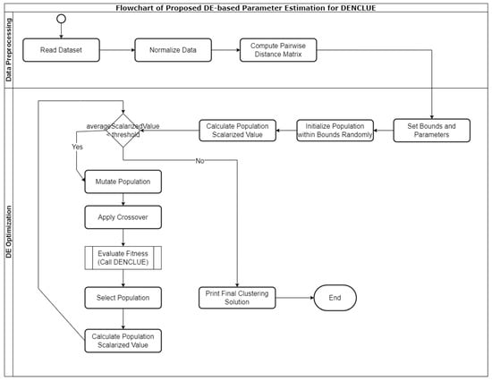
Figure 1.
Flowchart of the Proposed Approach.
Table 2.
Pseudocode for the Proposed Method.
3.1. Data Preprocessing
The dataset is normalised so all attributes are in the range [0, 1]. Next, the pairwise distance matrix is computed as it will be used extensively during optimisation. This pre-calculation of the distance matrix reduces the algorithm’s computational demands at different iterations of the optimisation process.
3.2. DE-Based Optimisation Process
In the context of DENCLUE parameter estimation, the DE algorithm’s standard operators (mutation, crossover and selection) are customised and modified to suit the specific requirements of parameter estimation. By exploiting this inherent capability to perform a thorough exploration of the entire search space for the parameters and not relying on any assumptions about the underlying data distributions, these adaptations aim to enhance the effectiveness of the parameter estimation process and improve the algorithm’s performance in handling clustering scenarios. The DE/rand/1/bin scheme was selected for parameter estimation in the DENCLUE algorithm due to its simplicity and ease of implementation [,]. This choice aims to make it applicable to various datasets and clustering scenarios.
3.2.1. Initialisation
The population comprises NP candidate solutions, each represented by a two-dimensional vector. The first dimension, sigma (σ), is a continuous value representing the influence range, while the second dimension, MinPts (ξ), is an integer. Such a solution is represented as . This setup addresses mixed integer-continuous optimisation, simplified to continuous optimisation []. The initial population is generated through uniform random initialisation within predefined bounds for both parameters, using Equation (3). The bounds for σ are set as [0, 1] and for the ξ as [2, nPoints], where nPoints is the number of data points in the dataset.
3.2.2. Optimisation Cycle
The DE iteratively mutates, applies crossover and selects the individuals based on their fitness value. Following the DE/rand/1/bin scheme, the mutation involves selecting a single difference vector between two randomly chosen individuals from the population. The binomial crossover strategy scheme is selected for simplicity and reduced computational complexity, complementing the straightforward mutation operator. The control parameter in Equation (4) defines the amplification of the difference vector in the mutation, while the parameter crossover probability, also known as crossover rate, CR in Equation (5), defines the probability of each parameter in the trial vector being inherited from the mutant vector rather than the target vector. After creating the trial vector through crossover, the selection operation determines whether the trial vector or the original target vector should proceed to the next generation based on their fitness values. By favouring the better-performing candidate solution, the selection operator aids convergence toward optimal solutions.
3.2.3. Fitness Evaluation
The objective function of the proposed method integrates two primary aspects: the internal clustering validation measures and the cluster coverage, i.e., the percentage of data clustered effectively to capture the density-based structure of data through effective clustering.
The rationale for including cluster coverage is to ensure that the algorithm identifies meaningful groups and maximises data inclusion within these clusters. Emphasising cluster coverage enhances clustering completeness, reducing un-clustered points and improving robustness. While external validation metrics, like the Adjusted Rand Index (ARI) [], and internal clustering validation metrics, such as the Silhouette Index (SI) [] and Davies–Bouldin Index (DBI) [], are widely used to assess clustering quality, they primarily focus on how well-separated or well-aligned the clustered data is. These metrics do not account for the proportion of data that is clustered [,]. Consider a scenario where only a small fraction of the dataset is clustered, yielding good ARI, SI and DBI values. Although numerically satisfactory, this situation is often impractical because it leaves a significant portion of the data un-clustered. This is particularly important when the clustering process progresses without user involvement and when visualising the intermediate clustering outcomes is not feasible []. Conversely, prioritising cluster coverage alone might lead to many small, poor-quality clusters.
In addition to cluster coverage, the proposed approach uses clustering quality as part of the objective function and combines the two elements into a scalarised fitness value. The main task is unsupervised learning; therefore, only internal clustering quality metrics are applicable. However, most internal clustering quality metrics are not suitable for datasets with arbitrarily shaped clusters [,]; therefore, specific measures like Density-based Clustering Validation (DBCV) [] are more appropriate. The DBCV index is preferred over other measures as it evaluates the clustering by considering the density distribution of data points within clusters. Another notable characteristic of DBCV is that it handles noise implicitly and effectively identifies clusters based on density sparseness and density separation. These characteristics make DBCV highly suitable for datasets with clusters of arbitrary shapes and varying densities, which aligns well with the goal of this study. The ability of DBCV to handle noise and its sensitivity to density variations ensures a more reliable clustering quality assessment, reinforcing the effectiveness of the parameter estimation process.
Density sparseness finds the areas within a cluster having the lowest density, whereas density separation measures the highest density regions between adjacent clusters. The validity index for a cluster () is computed through Equation (7), while the overall DBCV index for a clustering solution is computed through Equation (8).
The and in Equation (7) are two distinct clusters and k is the number of clusters in clustering solution . Likewise, in Equation (8) represents a cluster, is the validity index computed through Equation (7) and represents the total number of data points in the dataset.
The alignment of the DBCV index with the principles of DENCLUE ensures that the presented technique not only effectively estimates parameters but also achieves meaningful and practical clustering outcomes. The DBCV ranges from to , where higher values denote better clustering quality, providing a clear and quantitative measure of the effectiveness of the clustering process under study.
The DBCV and cluster coverage for clustering solution are combined into a scalalrised fitness value for each candidate solution, and is calculated through Equation (9). Consequently, Equation (10) (adapted from Equation (6)) represents the selection operator in the DE.
Here, represents the clustering validation measure for the candidate solution and is the percentage of data clustered by this solution, both normalised within the population. Weights () are assigned using the Pareto Ranking [] method, which helps prioritise solutions that balance effectively both objectives, identifying non-dominated solutions within the multi-objective context. This method ensures that no solution is improved at the expense of another, promoting an optimal balance between cluster quality and coverage.
3.2.4. Algorithm Termination
In the proposed optimisation process using Differential Evolution, the scalarised value of each individual in the population represents a composite measure combining the density-based clustering validation and the cluster coverage. As the generations progress, the DE algorithm refines the individuals in the population aiming to maximise these scalarised values. The behaviour of these values across generations can typically be described as follows:
- 1.
- Initial Generations
Early in the optimisation process, the scalarised values may show a wide range of variability. This is because the initial population is generated randomly; thus, the quality of solutions (individuals) can vary significantly. During these generations, the algorithm identifies potentially good solutions that provide a foundation for further refinement.
- 2.
- Mid-Generations
As the optimisation continues, the DE algorithm applies its operators—mutation, crossover and selection—to evolve the population. This phase often sees a general upward trend in the average scalarised values as sub-optimal solutions are gradually replaced by more promising ones. The improvements in these generations are crucial as they reflect the algorithm’s ability to explore and exploit the search space effectively.
- 3.
- Convergence Approach
The increase in scalarised values tends to plateau toward the later generations, indicating that the population converges towards a set of optimal or near-optimal solutions. This stabilisation occurs because further modifications to the individuals result in smaller incremental improvements or maintain the existing quality of solutions.
The termination criteria for the algorithm are set based on minimal improvements (less than a preset threshold) in the objective function values across consecutive iterations. Other stopping criteria include maximum number of generations, number of objective function evaluations [,], which are not suitable for the proposed method to work for a variety of data structures with diverse characteristics. The threshold is set based on empirical data across various datasets, indicating robust clustering performance at this level and an efficiently balanced performance with computational effort, avoiding unnecessary computational expense.
3.3. Computational Complexity of the Proposed Method
The proposed DE-based DENCLUE optimisation approach has three main components: the DE, DENCLUE and the DBCV. Based on these three main components, the time and space complexity of the method is derived as follows:
3.3.1. Time Complexity
For a D-dimensional dataset with N data points, the time complexity for the major steps, as shown in the pseudocode, is computed as:
- The time complexity of the Reading dataset file is
- The normalisation process also has a complexity of
- Computing pairwise distance matrix is a relatively costly operation and is
- For DE optimisation
- Initialisation is , where NP is the size of the population, and D is the number of variables in DE. Here NP is taken as 20 and D is 2 since there are two variables in DE; the sigma and the minimum density level/minpts.
- Mutation, crossover and selection are all
- Evaluating fitness for the population is multiplied by the inner operations
- (1)
- calling DENCLUE is
- (2)
- calling DBCV is also
- (3)
- calculating coverage is
Given the above, the dominant terms inside the DE optimisation loop are for the DENCLUE and and the loop iterates for NP population individuals. Therefore, the time complexity for the DE optimisation loop is . Adding the complexities of all the steps, the dominant term is the one inside the DE optimisation loop, especially when the number of data points, N, is large. Given NP = 20 and D = 2, it does not change the complexity, as they are constants. Therefore, the overall time complexity for the proposed method is .
3.3.2. Space Complexity
Considering the data points, the pairwise distance matrix and the population of the DE algorithm, the space complexity for the dataset is , for the pairwise distance matrix it is and for the Population in DE it is. Clearly, the dominant term is the pairwise distance matrix, leading to an overall space complexity of.
4. Results
4.1. Experimental Setup
This section outlines the experimental setup employed to assess the proposed method. The description begins with an overview of diverse synthetic and real datasets carefully selected to comprehensively assess the proposed method’s performance. Later, the performance validation criteria are also detailed. Lastly, the setup for comparison with existing density-based methods as benchmark comparison are also listed. The key details of the experimental setup encompass the parameter configurations for DE and its application in automatically estimating the DENCLUE’s input parameters.
4.1.1. Dataset Description
A diverse set of synthetic and real datasets were selected to comprehensively evaluate the proposed method’s performance across various scenarios. The synthetic datasets included Aggregation, Two Moons, Shapes, Spiral, Path-based, Zahn Compound and a carefully selected subset of S2 and A3 (to preserve the complexity of the dataset) from a publicly available clustering benchmark repository []. All the synthetic datasets used in this study were two-dimensional and selected to demonstrate the efficacy of the proposed clustering method in terms of its capability to handle challenges: (1) from simple geometric shapes to complex patterns with varying densities, such as Aggregation and Zahn’s Compound datasets, which have sub-clusters of diverse shapes; (2) Path-based shapes that typically have poorly separated clusters due to their closeness to each other; (3) a large number of clusters—for instance, the A3 dataset, which has several clusters; (4) overlapping clusters—for instance, S2, which has overlapping samples across clusters. The synthetic datasets used in this study have been widely used as benchmarks for density-based clustering techniques to demonstrate identifying clusters of arbitrary shapes, sizes and densities [,,,,].
The real-world benchmark datasets used were IRIS, Heart Disease, Seeds and Wine obtained from the UCI Machine Learning repository [] and cover different domains, such as biology, healthcare and agriculture, ensuring a balanced and extensive evaluation of the clustering method. While the synthetic datasets, all two-dimensional, represent the inherent complexity in cluster structures, the real-world datasets have increased dimensionality and cluster overlap [,,,,,,]. The inherent noise and outliers in the real-world dataset are common characteristics reflecting realistic scenarios the proposed method is designed to handle. However, a detailed study of the proposed method under artificially injected varying noise levels has been submitted as a separate study and is currently under review. Table 3 lists the details of the datasets used, including the number of instances (sample size), the number of features (dimensionality), the number of true clusters and the rationale behind their selection.
Table 3.
Description of Datasets Used.
4.1.2. Setting Control Parameters for DE
Before applying the approach to estimate the parameters of the DENCLUE algorithm, it was crucial to configure the control parameters of the DE algorithm. The DE algorithm relies on two key parameters: the mutation scaling factor (F) and the crossover rate (CR). The choice of these parameters can significantly influence the performance of the DE algorithm and, subsequently, the parameter estimation process for the DENCLUE. A suitable range of values/combinations for F and CR was defined to ensure a comprehensive search within reasonable bounds. The choice of F as 0.5 was motivated by its common usage in DE and its balanced impact on mutation [,]. To explore the impact of the crossover rate (CR), a suitable range of values in were selected for experiments, as shown in Table 4. Population Size (NP) as suggested by [] was set to be 5 to 10 times the number of dimensions of the DE; for two variables σ and ξ, the population size was set as 20. Each combination was run five times to assess the consistency and reliability of the results.
Table 4.
Parameter Range for DE.
Once the DE parameters are set, the algorithm undergoes execution, and while executing, it documents outcomes for every repetition across parameter combinations. These detailed results encapsulate the optimisation data for convergence analysis, including Generation, the influence range parameter (σ), the minimum density level parameter (ξ), DBCV, Coverage and the fitness value for each individual across generations. Next, the mean generations required to reach the termination criteria for each combination were recorded. Along with the mean, standard deviation is also computed. This analytical process contributes to carefully selecting optimal F and CR parameters for DENCLUE parameter estimation.
4.1.3. Parameter Ranges for DENCLUE
The proposed algorithm estimates the DENCLUE algorithm’s parameters for each dataset using DE’s pre-configured parameters through experiments. An initial range, serving as the search space for each of the DENCLUE parameters σ and ξ, is defined, and the optimisation is applied. The wide range of values ensures an extensive search space that covers a diverse set of potential parameter values. This broad exploration is crucial as it eliminates the need for domain-specific knowledge or user input, allowing the optimisation process to naturally adapt to the dataset’s properties. Table 5 presents the parameter settings for the DENCLUE parameter estimation experiments. To further validate the robustness of the presented technique, the experiments were repeated five different times/runs.
Table 5.
Parameter Ranges for DENCLUE.
4.1.4. Evaluation Metrics
The objective for evaluating the quality of clustering is to assess the effectiveness and reliability of DENCLUE parameters estimated by the proposed method. The following clustering quality metrics have been used in the evaluation due to their widespread adoption in clustering validation [,,]. The Silhouette Score (SI) measures how closely related an object is to others within its cluster compared to those in different clusters, ranging from [−1, 1] with higher scores indicating well-defined clusters. The Davies–Bouldin Index (DBI) assesses cluster separation by comparing the similarity between each cluster and its most similar counterpart, where lower values indicate better separation. The Adjusted Rand Index (ARI) quantifies the agreement between true class labels and clustering results, normalised to account for chance, ranging from [−1, 1], with higher values signifying more accurate clustering.
4.1.5. Comparison with Existing Density-Based Methods
The proposed method will be compared with established benchmark methods in density-based clustering to highlight the effectiveness and advantages of the approach in automating parameter optimisation and improving clustering accuracy. Density-based clustering algorithms are crucial for identifying patterns and structures in complex datasets. Among the various density-based clustering methods, DPCSA [] and VDENCLUE [] demonstrate significant potential in handling density-based clustering challenges. DPCSA offers improved accuracy and reduced manual parameter tuning, while VDENCLUE addresses clustering in datasets with varying densities through variable Kernel Density Estimation.
DPCSA’s code is available (https://github.com/Yu123456/DPCSA, accessed on 20 August 2024), allowing for a direct and fair comparison of clustering performance. The availability of code enabled benchmarking the presented technique against a well-regarded density-based approach without concerns about implementation discrepancies. VDENCLUE’s code was not publicly available; however, its relatively straightforward implementation motivated its inclusion in the evaluation. By custom implementation of VDENCLUE (made publicly available (https://github.com/omerdotajmal/vdenclue, accessed on 20 August 2024) for fair comparison), the evaluation ensured a robust comparison that accounts for its advancements in handling datasets with varying densities.
The DPCSA method uses KNN to redefine the local density, and the value of K is set as 5 by the authors, which will also be the same value used for comparison here. DPCSA also requires a user to select a region of interest for minimum local density threshold ρ, and min. distance from higher density point δ. Five regions of interest with minimal overlap (not more than 10%) are selected in the experiments. VDENCLUE takes two parameters: the nearest neighbour points used in the density estimation, k and the minimum density level ξ. The authors suggest k and ξ range from 4 to 12 for best results. For comparison, VDENCLUE is run for all values between the intervals specified by its authors.
4.1.6. Software and Hardware Setup
The experimental setup utilised Java (version SE-15) for its robust libraries, and the Eclipse IDE was used to manage the coding process. The experiments were run on a Windows 10 system with an Intel Core i5 processor and 8 GB RAM. Java libraries and custom scripts were used for preprocessing, while Seaborn in Python (version 3.12.3) was used for data visualisation. The DPCSA Matlab code was obtained from Github online (accessed on 20 August 2024) and executed using Matlab (version R2024a) online, while VDENCLUE was implemented in Python (version 3.12.3).
4.2. Results for DE Parameters Selection
The experiments for DE parameter selection involved calculating the mean number of generations needed to reach the maximum scalarised objective value for each DE run combination, providing insight into convergence speed. The standard deviation was also computed to assess consistency across repetitions. The fitness achieved by each DE run combination was evaluated by comparing the maximum scalarised values. Table A1 in the Appendix A shows the top five DE run combinations based on the mean and standard deviation of generations to reach the threshold fitness value for each synthetic dataset, and Table A2 shows the same for real datasets.
No single DE run was found to be the best for all datasets. However, lower mean values were observed for the shapes and moons dataset because, in most repetitions of a DE run combination, the maximum fitness value was found in the initial population, i.e., Generation −1. Both of the Shapes and Two Moons datasets had clusters that were well separated. By analysing the top five best DE Run combinations for both real and synthetic datasets, the DE run 16 (F = 0.5, CR = 0.8) occurs in most datasets with low mean and standard deviation values. The choice of the DE run combination also depends on the dataset characteristics. However, the combination F = 0.5 and CR = 0.8 is suitable for most datasets. These values of F and CR also conform to the observation made by [] for non-separable functions (dependent parameters) and in achieving satisfactory results in most cases, as suggested by []. The proposed algorithm subsequently uses the optimised DE parameters.
4.3. Results for DE-Based DENCLUE Parameters Estimation
DENCLUE parameter estimation experiments were repeated five times for all datasets to validate the presented technique’s robustness. Additionally, the clustering quality was validated by three validation measures, i.e., Silhouette (SI), Davies–Bouldin Index (DBI) and Adjusted Rand Index (ARI). It is worth highlighting a notable observation before interpreting the results for each dataset. For datasets containing clusters with highly varying densities, shape sizes and cluster overlaps, the DBCV values for ground truth clustering tend to be low, i.e., close to −1; conversely, in cases where clusters are well-separated, the DBCV values tend to be higher, i.e., close to +1. The DBCV as part of the objective aims to find clusters that align with the underlying density-based structure of the data. High SI values and low DBI values indicate more compact and better separated clusters; however, these might not always align with the underlying density-based structure. The results for the proposed method, along with DPCSA and VDENCLUE, are shown in Table 6.
Table 6.
Comparison of Clustering Performance Metrics across Methods.
Details of the five runs for synthetic datasets by the proposed method are shown in Table A3, Table A4, Table A5, Table A6, Table A7, Table A8, Table A9 and Table A10 (Appendix A), which helps the reader understand the stability of the proposed method across different runs. Figure 2 presents the visualisations of the clustering produced by the proposed method and the other two benchmark methods for synthetic datasets, while Figure A1, Figure A2, Figure A3, Figure A4, Figure A5, Figure A6, Figure A7 and Figure A8 in Appendix A present the clustering visualisations for all five runs by the proposed method.
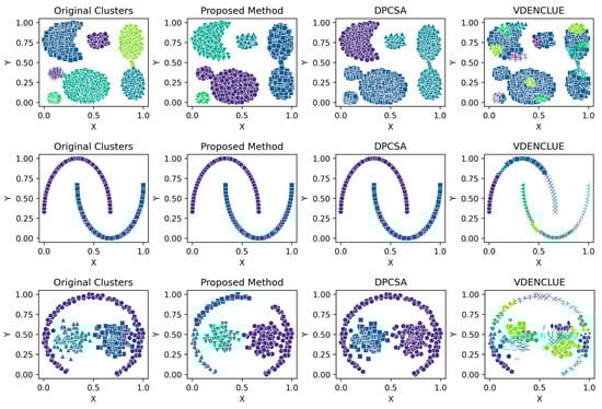
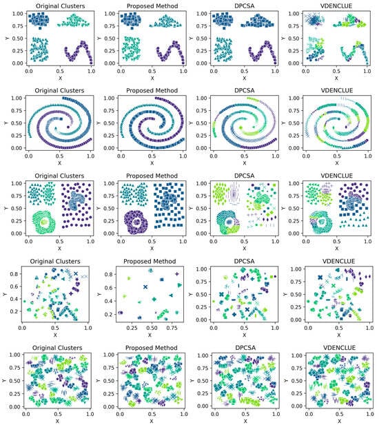
Figure 2.
Visualisations of Clustering by Different Methods—Synthetic Datasets. From Top to Bottom: Aggregation, Moons, Path-based, Shapes, Spiral, Zahn’s Compound, S2 and A3. Each cluster is shown in a unique colour and marker.
The aggregation dataset has seven true clusters, with two pairs of clusters close together. The clusters are of a complex shape and vary in sizes and densities. The parameters learned through the presented technique produced stable DBCV values, except for Run 1, which had the lowest DBCV. Also, the presented technique produced a high ARI and Coverage of 1.00, indicating good cluster assignment. While the clusters produced by the proposed method align well with the true underlying structure (as confirmed by the highest ARI achieved), the clusters themselves are not well-separated and have overlapping regions, resulting in lower SI and higher DBI values. In comparison, clusters produced by DPCSA have higher SI and lower DBI, yet the clustering does not align with the actual underlying density-based structure of the dataset.
The moon dataset has two interweaved clusters. The results show stable performance across runs, validating the robustness of the proposed method. The ARI and SI are the highest among the counterparts. The high DBI by the proposed method, as compared to VDENCLUE, shows that the clusters produced are well-separated yet differ from the true underlying structure, as confirmed by a very low ARI value. The same phenomenon can be observed for the path-based dataset characterized by three clusters, one large cluster and two smaller clusters close to the larger one, leading to poor separation resulting in higher DBI values for the proposed method.
For the shapes dataset, the clustering produced by the proposed method resulted in superior clustering compared to its counterparts. The spiral dataset is characterized by three interweaved clusters that are not well separated. Despite poor separation, the proposed method achieved perfect clustering with an ARI value of 1.0, considerably higher than its counterparts. This further confirms the effectiveness of the DBCV as part of the objective function, as maximizing it helps detect the true underlying density-based structure.
Zahn’s compound dataset features six distinct clusters with significant variations in density, shape and size, posing a challenge for clustering algorithms like DENCLUE, which rely on a single global influence range parameter. The proposed method better aligns with the true structure than its counterparts, as confirmed by considerably higher ARI and SI values. The higher DBI by the proposed method reflects that clusters are close to each other and not distinct, leading to less clear boundaries between them. For the complex S2 dataset, the proposed method yielded the best clustering, with clusters aligning close to the true structure, and all three clustering metrics being superior to the counterparts. However, the data points clustered remained low i.e., 86% coverage.
The A3 dataset has 50 clusters, which poses significant challenges for density-based clustering methods. The complexity inherently impacts the DBCV scores across multiple runs of the dataset. The ARI produced by all three methods is high, with VDENCLUE having a slight advantage due to its varying KDE approach. However, the proposed method produced higher ARI and clusters that closely aligned with the true structure. Most runs achieved high ARI with high coverage (Table A10), demonstrating instances where the clustering method was effective in grouping data despite challenging conditions.
It is worth mentioning that the proposed DE-based DENCLUE parameter estimation approach targets optimising DBCV with Cluster Coverage as the primary objectives. However, the robustness and effectiveness of the approach are contingent on its performance across various dimensions. The analyses of how DBCV correlates with other external and internal validation metrics, i.e., ARI, SI and DBI, will help the reader understand their nuanced relationship and the effectiveness of the proposed method. A high correlation is expected between DBCV and SI, DBCV and ARI, and a low correlation between DBCV and DBI. The correlation ranges from −1 to +1, with higher values corresponding to positive correlation and vice versa. The correlation heatmaps, along with significance (p-value) and confidence interval for synthetic datasets, are shown in Figure A9, Figure A10, Figure A11, Figure A12, Figure A13, Figure A14, Figure A15 and Figure A16 in Appendix A. A p-value < 0.5 indicate a significant correlation, while confidence intervals represent the range within which the true correlation is likely (with 95% confidence) to lie. From the correlation matrices, it becomes evident that, for all synthetic datasets, there is a positive correlation between DBCV and ARI, DBCV and SI. Similarly, a negative correlation between DBCV and DBI further validates the presented technique’s effectiveness in optimising high-quality clustering solutions. The low but positive correlation values for moons and path-based datasets are attributed to the fact that most of the solutions generated by the presented technique produced the same ARI, with minimal variations in the DBCV values, as shown by the distribution of values in Figure A17 and Figure A18.
The clustering results of the proposed method on real datasets for all runs are shown in Table A11, Table A12, Table A13 and Table A14 (Appendix A). The correlation heatmaps are shown in Figure A29, Figure A30, Figure A31 and Figure A32 (Appendix A). The IRIS dataset is characterized by three clusters, two of which overlap each other due to the inherent overlap in the features space (Figure A19, Appendix A). The clustering produced by the proposed method resulted in the highest ARI and SI values as compared to its counterparts, although none of the three methods was able to detect all three clusters due to significant cluster overlap. The low DBI values further confirm the efficiency of the presented technique. The ARI values are reasonable as well, though not ideal. The results across multiple runs are stable, supporting the optimisation approach’s robustness.
The Heart Disease dataset presented a challenge to all three methods as it contains a relatively large number of dimensions. The number of clusters and substantial overlap between clusters in several dimensions (Figure A20, Figure A21, Figure A22 and Figure A23, Appendix A) also add to the complexity. However, the presented technique exhibits noteworthy stability across various metrics in all runs, including DBCV, SI, DBI and ARI. Additionally, the number of clusters and DENCLUE parameter values remain reasonably consistent, further underscoring the robustness of the presented technique. Nevertheless, the challenges encountered in achieving efficient clustering in this context open exciting avenues for exploring novel solutions to address such complex scenarios. VDENCLUE achieved the highest ARI among competitors with clusters because of its variable bandwidth in KDE, which allows it to fine-tune its clustering process more accurately for datasets with clusters with minimal separation. This enables VDENCLUE to differentiate small differences between overlapping clusters better. It lacks, however, good SI and DBI values.
The Seeds dataset also contains overlapping clusters (Figure A24 and Figure A25, Appendix A). The DBCV values produced by the proposed method showed fluctuations across multiple runs, indicating varying clustering qualities (Table A13). The coverage remains consistently high, indicating that clusters cover most data points. However, the ARI values remain relatively low, while counterparts performed relatively better. The lower SI and higher DBI are due to the overestimation of clusters. The main reason for the performance degradation of the proposed method in the Seeds dataset lies in how the DBCV metric evaluates the clustering quality. The DBCV value for the true structure of the Seeds dataset is considerably low at −0.3468, whereas the proposed method pushes the clustering process towards configurations that result in high DBCV values. Therefore, the proposed method may have prioritised more internally dense clusters and attempted to force separation even when natural clusters overlapped significantly. Nevertheless, despite the challenges in achieving efficient clustering, the proposed method demonstrates stability regarding DBCV, SI, DBI and the number of clusters in most runs. This consistency underscores the robustness of the approach, even in the face of dataset complexities like those presented by the Seeds dataset.
The Wine dataset, with its 13 attributes, posed a considerable challenge to the presented technique. Notably, significant overlap was observed between at least 10 pairs of features (some of which are depicted in Figure A26, Figure A27 and Figure A28), making it a complex dataset for clustering. The proposed method achieved the highest SI values among counterparts, with ARI second only to VDENCLUE. Clearly, none of the three methods is superior in all three metrics. Nevertheless, the stability of key metrics and parameter values across runs (Table A14) underscores the robustness of the presented technique.
Despite the challenging structures for the real datasets, the use of DBCV as part of the objective function to optimise is validated by the results for the correlation of DBCV with other validation metrics for real datasets (as depicted in Figure A29, Figure A30, Figure A31 and Figure A32).
The correlation matrices for the IRIS and Wine datasets show high positive correlations between DBCV and SI, moderate to high correlations with ARI and low to negative correlations between DBCV and DBI, confirming the overall effectiveness of DBCV as part of objective function even for real datasets. The Heart Disease and Seeds datasets exhibit a weak but positive correlation between DBCV and ARI, a strong positive correlation between the DBCV and SI and a negative correlation between DBCV and DBI, further adding to the overall effectiveness of the proposed optimisation method. In the Seeds dataset, the low ARI correlation indicates a challenge in aligning the clusters with the true labels, despite good overall cluster quality, as measured by the DBCV and SI of the optimisation method.
The proposed method’s overall consistent and effective performance in comparison to its counterparts is also further validated by analyses of the predicted vs. true clusters, and the best and average ARI achieved across multiple runs of the three methods. Figure 3 shows the cluster deviations of all three methods from the true clusters; whereas, Figure 4 and Figure 5 present the average and the best ARI, respectively, by each method. The proposed method exhibits high accuracy, closely matching the number of clusters across various datasets, while DPCSA and VDENCLUE often overestimating the clusters.
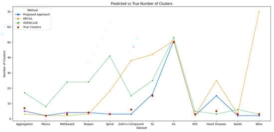
Figure 3.
Comparison of Predicted vs. True Clusters.
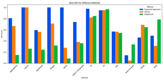
Figure 4.
Comparison of Best ARI.
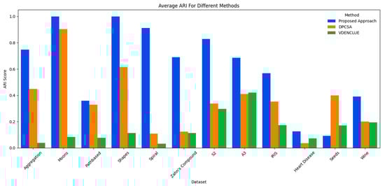
Figure 5.
Comparison of Average ARI.
The best and average ARI analyses further substantiate the overall superior performance of the proposed optimisation method for various datasets. This robust performance highlights the presented technique’s sophisticated optimisation process, particularly in managing complex data structures in datasets like Spiral and Zahn’s compound, where it significantly outperforms DPCSA and VDENCLUE. For the Heart Disease dataset containing significant cluster overlap in several dimensions, the average ARI for all three methods remains low, with the proposed method achieving the highest average ARI. For the IRIS dataset, the proposed method is superior to counterparts for both best and average ARI and superior to other methods for average ARI in the Wine dataset. However, for the Seeds dataset, where there is cluster overlap in certain dimensions, the proposed method underperforms compared to its counterparts.
These results indicate that the proposed method is superior to the benchmark methods for most synthetic and real-world datasets containing clusters of different sizes, densities, shapes, degrees of overlap and number of clusters. The proposed method’s superior performance over the benchmark methods is attributed the following factors:
- It learns the parameters of the clustering algorithm automatically, adapting to the dataset characteristics, whereas both DPCSA and VDENCLUE require the user to carefully select the input parameters, and the choice of the parameters significantly affects their clustering outcomes.
- It is based on DENCLUE, which is effective in handling complex data structures with inherent noise.
- It uses the density-based clustering validation (DBCV) index as part of its optimisation’s objective function. The validation index is specifically designed to promote density-based clustering, detecting clusters of varying, shapes, sizes and densities.
However, the proposed method struggles in scenarios such as:
- The datasets containing clusters not well-separated or having significant overlap in them, as shown by the inferior performance of Heart Disease and Seeds datasets. This limitation is inherent to the use of DBCV [];
- High-dimensional datasets, as the computational complexity of the proposed method is relatively high compared to the benchmark methods. Also, the method is not suitable for simple datasets where the effective parameters fall within a narrow range, since the introduced computational overhead is not worth it; some simple grid-based search techniques for parameter estimation will be appropriate.
- The proposed method’s performance is dependent on how the DENCLUE algorithm detects the clusters. Even when the right parameters are estimated, DENCLUE’s limitation of using a single global density threshold and influence range parameter limits its applicability to the datasets where a cluster has inner density variations. VDENCLUE, however, handles this well due to its varying kernel density estimation approach.
5. Discussion
The findings from this study provide sufficiently strong evidence for the effectiveness of using DE to optimise DENCLUE parameters, especially in complex datasets. This helps to overcome the limitations associated with traditional trial-and-error approaches or heuristic-based approaches, offering a more systematic and robust parameter estimation process. The results confirm the proposed method’s adaptability and robustness across various synthetic and real datasets.
The standard DENCLUE algorithm is sensitive to initial parameters (the influence range parameter σ and the density threshold ξ) for retrieving true clusters. A user often chooses these parameters with a trial-and-error approach [,,]. Another challenge observed is that there is no single set of parameters that is suitable across all datasets, so users have to run experiments with different combinations of these parameter values across datasets to achieve the required dataset clustering quality, which is either measured in terms of clustering quality metrics such as DBCV, SI, DBI and ARI or through visual analysis for two-dimensional and three-dimensional datasets. The literature demonstrates that to handle such a problem, grid-search approaches are adopted for the optimal parameters instead of a trial-and-error mechanism [,,,,]. We performed experiments using this grid-search approach for original DENCLUE to analyse its effectiveness and observed that, in some cases, the results were not satisfactory, suggesting it requires a different grid-size to get optimal clustering results in capturing the underlying true clusters. In contrast, the proposed method enhances the original DENCLUE by exploiting the DE optimisation technique to estimate optimal parameters automatically for extracting accurate clusters in a dataset. A comparison between grid-search and the proposed method across datasets is presented in Appendix B.
The choice of DE control parameters, validated through experiments, conforms to those suitable for multi-objective optimisation of non-separable functions []. The choice proved to be suitable for exploring the diverse parameters for DENCLUE, resulting in effective clustering on a variety of datasets. In their analysis of the most frequently used parameter values for F and CR, and widely used performance measures in DE and its variants, Ahmad et al. [] reported F = 0.5 and CR in [0.8, 1] as the most commonly used values. Moreover, the authors also reported mean and standard deviation as the widely accepted choices for performance measures. However, more sophisticated techniques with adaptive mutation and crossover are available. Adaptive DE variants [] and a more detailed sensitivity analysis using metrics relevant to multi-objective optimisation [] will be explored in subsequent research on the proposed method.
The DBCV, as part of the multi-objective of the proposed method, proved to be effective for most datasets. The DBCV, specifically designed for density-based clustering and inherent handling of noise, made it a preferred choice over other competitors. This is validated by the analyses of the correlation between DBCV and the other two internal clustering validation metrics, i.e., SI and DBI. The correlation of DBCV with SI is lower in datasets containing complex structures like Aggregation, Spiral and Zahn’s compound than datasets containing well-separated clusters. This indicates that while maximizing the DBCV made the detection of true underlying structure successful, the SI measure for the true cluster structure remained low []. A similar phenomenon was observed for weak negative correlation with DBI. In the subsequent research for the proposed method, other validation indices suitable for arbitrarily shaped clusters and with significant overlap will be explored to enhance the objective function in the hope of better detecting clusters in very complex structures like Heart Disease and Seeds.
DPCSA and VDENCLUE, while showing strengths in certain datasets, require careful selection of parameters to achieve optimal performance. DPCSA, for example, often overestimates the number of clusters due to its sensitivity to local density peaks. This method depends heavily on the appropriate choice of cutoff distances and density thresholds, which can vary significantly between datasets and may lead to poor clustering outcomes if not selected carefully. Similarly, while VDENCLUE’s variable bandwidth offers flexibility, it also introduces parameter sensitivity that requires fine-tuning to avoid misclassification or overfitting to noise. This dependency on precise parameter tuning highlights a crucial advantage of the proposed method, significantly reducing the risk of human error and ensuring more consistent and reliable clustering results. This level of automation is particularly valuable in practical applications where reproducibility and ease of use are critical, making the proposed method a preferred choice for scenarios demanding high reliability without extensive manual tuning.
Key contributions by the method presented in this article include (1) introduction of a novel application of DE for optimising DENCLUE parameters; (2) the study pioneers cluster coverage as an optimisation objective, enhancing the practical utility of clustering beyond traditional validation metrics, and it demonstrates empirically that relying solely on conventional clustering quality metrics is insufficient for practical applications, especially for an automated approach where the intermediate clustering outcomes are optimised without user feedback, thus advocating for a multi-objective optimisation approach that better addresses real-world data complexities; (3) this approach advances the principles of Automated Machine Learning (AutoML), simplifying the model selection and parameter tuning processes, thereby making sophisticated clustering methodologies accessible to a broader audience without requiring deep domain-specific knowledge.
The proposed DE-based DENCLUE parameters estimation approach has shown reasonable performance across various real datasets. The acknowledged limitations are datasets with significantly overlapping clusters and potential challenges with very high-dimensional or large-scale datasets due to increased computational complexity. Future research directions include implementing adaptive variants of DE, use of other clustering metrics as objective and parallel implementation of the proposed method to better handle high dimensional and large-scale datasets.
6. Conclusions
One of the key challenges in density-based clustering algorithms such as DENCLUE is the selection of appropriate parameters. Traditionally, the selection of optimal parameters relies on trial-and-error, heuristics-based approaches, and usually require some sort of knowledge about the underlying data distribution. In complex datasets, containing varying densities, sizes, shapes and noise, estimating the correct parameters becomes even more challenging as incorrect parameters may significantly affect clustering performance. The proposed method addressed the issue of optimising DENCLUE parameters through Differential Evolution, overcoming the limitations of existing methods. The proposed method eliminates the need for domain knowledge and manual tuning, offering an adaptable, robust, systematic and automated approach to parameter estimation, superior to selected counterparts, particularly for datasets with well-separated clusters of arbitrary shapes. The acknowledged limitations in identifying overlapping clusters will be addressed in future research through applying adaptive DE variants and additional density-based clustering validation metrics to further improve clustering performance, particularly in high-dimensional and noisy datasets and complex structures with overlap.
Author Contributions
Conceptualization, O.A. and S.M.; Data curation, O.A. and T.H.; Formal analysis, O.A.; Funding acquisition, T.H., R.W.A. and A.A.; Investigation, O.A.; Methodology, O.A., S.M. and H.A.; Project administration, H.A. and T.H.; Resources, A.S., T.H. and R.W.A.; Software, O.A. and A.S.; Supervision, S.M. and H.A.; Validation, O.A., S.M. and H.A.; Visualization, O.A. and T.H.; Writing—original draft, O.A.; Writing—review & editing, T.H., R.W.A. and A.A. All authors have read and agreed to the published version of the manuscript.
Funding
Princess Nourah bint Abdulrahman University Researchers Supporting Project number (PNURSP2024R 343), Princess Nourah bint Abdulrahman University, Riyadh, Saudi Arabia. The authors also extend their appreciation to the Deanship of Scientific Research at Northern Border University, Arar, KSA for funding this research work through the project number “NBU-FFR-2024-1092-08”.
Institutional Review Board Statement
Not applicable.
Data Availability Statement
The original data presented in the study are openly available at http://cs.uef.fi/sipu/datasets/ (accessed on 20 August 2024) and https://archive.ics.uci.edu (accessed on 20 August 2024). The code is available under CC BY 4.0 license at https://github.com/omerdotajmal/mulobjdenclue (accessed on 20 August 2024).
Conflicts of Interest
The authors declare no conflicts of interest.
Appendix A
Table A1.
Top Five DE Run Combinations for Synthetic Datasets: Each column shows the mean generations to reach the threshold and the standard deviation for the top five DE parameter combinations.
Table A1.
Top Five DE Run Combinations for Synthetic Datasets: Each column shows the mean generations to reach the threshold and the standard deviation for the top five DE parameter combinations.
| DE Run | Dataset | Aggregation | Two Moons | Path-Based | Shapes | Spiral | Zahn’s Compound | S2 | A3 |
|---|---|---|---|---|---|---|---|---|---|
| DE Run 2 | 2.60, 4.97 | 2.00, 2.00 | |||||||
| DE Run 3 | 0.60, 3.58 | 1.50, 1.30 | |||||||
| DE Run 5 | 2.10, 1.65 | ||||||||
| DE Run 6 | −0.40, 1.34 | 7.80, 14.34 | |||||||
| DE Run 7 | 1.85, 1.75 | ||||||||
| DE Run 8 | 1.75, 2.00 | ||||||||
| DE Run 9 | −0.80, 0.45 | −0.40, 1.34 | |||||||
| DE Run 11 | 1.40, 2.51 | −0.20, 1.30 | |||||||
| DE Run 13 | −0.20, 0.84 | 1.00, 1.87 | 1.40, 2.51 | 2.00, 1.90 | 2.00, 1.50 | ||||
| DE Run 14 | 3.20, 3.11 | −0.40, 0.89 | 3.20, 5.02 | ||||||
| DE Run 15 | 2.60, 4.34 | 0.00, 1.73 | |||||||
| De Run 16 | 3.20, 6.38 | 9.20, 5.17 | −0.40, 0.89 | 1.60, 2.88 | 1.00, 2.35 | 1.80, 1.20 | 1.65, 1.40 | ||
| DE Run 18 | 3.20, 4.66 | 10.20, 12.68 | 1.60, 3.29 | ||||||
| DE Run 19 | 0.00, 1.41 | 9.20, 10.69 | 2.05, 2.15 | ||||||
| DE Run 20 | 0.00, 1.22 | 0.00, 1.00 | 3.60, 3.71 | 2.25, 1.95 | |||||
Table A2.
Top Five DE Run Combinations for Real Datasets.
Table A2.
Top Five DE Run Combinations for Real Datasets.
| DE Run | Dataset | IRIS | Heart Disease | Seeds | Wine |
|---|---|---|---|---|---|
| DE Run 5 | 1.90, 1.40 | 1.80, 1.60 | 1.95, 1.70 | ||
| DE Run 7 | 2.00, 1.80 | 2.10, 1.90 | 4.00, 3.10 | ||
| DE Run 13 | 2.10, 1.70 | 2.20, 1.90 | |||
| DE Run 14 | 2.00, 1.75 | 3.50, 2.40 | |||
| DE Run 15 | 2.00, 1.60 | 1.80, 1.65 | |||
| De Run 16 | 1.70, 1.30 | 1.60, 1.20 | 1.75, 1.45 | ||
| DE Run 19 | 2.00, 1.85 | 3.60, 2.50 | 2.10, 1.90 | ||
| DE Run 20 | 1.85, 1.60 | 4.10, 3.20 | |||
Table A3.
Results for Synthetic Datasets—Aggregation.
Table A3.
Results for Synthetic Datasets—Aggregation.
| Aggregation | |||||||||
|---|---|---|---|---|---|---|---|---|---|
| Run | Gen | DBCV | Coverage | ARI | σ | ξ | SI | DBI | Clusters |
| 1 | 90 | −0.139 | 1.00 | 0.808 | 0.0810 | 16 | 0.374 | 0.905 | 5 |
| 2 | 74 | −0.104 | 1.00 | 0.733 | 0.1099 | 38 | 0.451 | 0.913 | 4 |
| 3 | 78 | −0.104 | 1.00 | 0.733 | 0.1058 | 28 | 0.451 | 0.913 | 4 |
| 4 | 127 | −0.104 | 1.00 | 0.733 | 0.0924 | 29 | 0.451 | 0.913 | 4 |
| 5 | 77 | −0.118 | 1.00 | 0.733 | 0.0889 | 20 | 0.451 | 0.913 | 4 |
Table A4.
Results for Synthetic Datasets—Two Moons.
Table A4.
Results for Synthetic Datasets—Two Moons.
| Two Moons | |||||||||
|---|---|---|---|---|---|---|---|---|---|
| Run | Gen | DBCV | Coverage | ARI | σ | ξ | SI | DBI | Clusters |
| 1 | 13 | 0.160 | 1.00 | 1.00 | 0.0604 | 2 | 0.390 | 1.338 | 2 |
| 2 | 23 | 0.160 | 1.00 | 1.00 | 0.0849 | 2 | 0.390 | 1.338 | 2 |
| 3 | −1 | 0.160 | 1.00 | 1.00 | 0.1439 | 7 | 0.390 | 1.338 | 2 |
| 4 | 10 | 0.160 | 1.00 | 1.00 | 0.2071 | 9 | 0.390 | 1.338 | 2 |
| 5 | −1 | 0.160 | 1.00 | 1.00 | 0.0545 | 2 | 0.390 | 1.338 | 2 |
Table A5.
Results for Synthetic Datasets—Path-based.
Table A5.
Results for Synthetic Datasets—Path-based.
| Path-Based | |||||||||
|---|---|---|---|---|---|---|---|---|---|
| Run | Gen | DBCV | Coverage | ARI | σ | ξ | SI | DBI | Clusters |
| 1 | 308 | −0.415 | 0.97 | 0.549 | 0.0615 | 4 | 0.458 | 1.192 | 4 |
| 2 | 281 | −0.597 | 1.00 | 0.0005 | 0.0827 | 2 | 0.0005 | 1.404 | 2 |
| 3 | 273 | −0.372 | 0.98 | 0.558 | 0.0551 | 3 | 0.285 | 1.463 | 9 |
| 4 | 410 | 0.018 | 0.94 | 0.0906 | 0.0224 | 2 | 0.484 | 1.102 | 64 |
| 5 | 983 | −0.426 | 0.93 | 0.593 | 0.0608 | 5 | 0.492 | 1.151 | 4 |
Table A6.
Results for Synthetic Datasets—Shapes.
Table A6.
Results for Synthetic Datasets—Shapes.
| Shapes | |||||||||
|---|---|---|---|---|---|---|---|---|---|
| Run | Gen | DBCV | Coverage | ARI | σ | ξ | SI | DBI | Clusters |
| 1 | 4 | 0.227 | 1.00 | 1.00 | 0.1865 | 3 | 0.701 | 0.585 | 4 |
| 2 | 6 | 0.227 | 1.00 | 1.00 | 0.0939 | 19 | 0.701 | 0.585 | 4 |
| 3 | 6 | 0.227 | 1.00 | 1.00 | 0.1173 | 17 | 0.701 | 0.585 | 4 |
| 4 | 5 | 0.227 | 1.00 | 1.00 | 0.1718 | 65 | 0.701 | 0.585 | 4 |
| 5 | 16 | 0.227 | 1.00 | 1.00 | 0.0755 | 16 | 0.701 | 0.585 | 4 |
Table A7.
Results for Synthetic Datasets—Spiral.
Table A7.
Results for Synthetic Datasets—Spiral.
| Spiral | |||||||||
|---|---|---|---|---|---|---|---|---|---|
| Run | Gen | DBCV | Coverage | ARI | σ | ξ | SI | DBI | Clusters |
| 1 | 136 | −0.226 | 1.00 | 1.00 | 0.1102 | 2 | 0.010 | 7.737 | 3 |
| 2 | 82 | −0.235 | 1.00 | 1.00 | 0.0423 | 2 | 0.010 | 7.737 | 3 |
| 3 | 56 | −0.433 | 1.00 | 0.56 | 0.1292 | 27 | 0.031 | 8.463 | 2 |
| 4 | 137 | −0.245 | 1.00 | 1.00 | 0.0955 | 12 | 0.010 | 7.737 | 3 |
| 5 | 120 | −0.235 | 1.00 | 1.00 | 0.1253 | 22 | 0.010 | 7.737 | 3 |
Table A8.
Results for Synthetic Datasets—Zahn’s Compound.
Table A8.
Results for Synthetic Datasets—Zahn’s Compound.
| Zahn’s Compound | |||||||||
|---|---|---|---|---|---|---|---|---|---|
| Run | Gen | DBCV | Coverage | ARI | σ | ξ | SI | DBI | Clusters |
| 1 | 42 | −0.097 | 1.00 | 0.740 | 0.1181 | 3 | 0.602 | 0.779 | 3 |
| 2 | 156 | −0.097 | 1.00 | 0.740 | 0.1182 | 7 | 0.602 | 0.779 | 3 |
| 3 | 84 | −0.100 | 1.00 | 0.740 | 0.1051 | 5 | 0.602 | 0.779 | 3 |
| 4 | 44 | −0.087 | 1.00 | 0.484 | 0.1460 | 23 | 0. 497 | 1.080 | 2 |
| 5 | 56 | −0.097 | 1.00 | 0.740 | 0.1093 | 3 | 0.602 | 0.779 | 3 |
Table A9.
Results for Synthetic Datasets—S2.
Table A9.
Results for Synthetic Datasets—S2.
| S2 | |||||||||
|---|---|---|---|---|---|---|---|---|---|
| Run | Gen | DBCV | Coverage | ARI | σ | ξ | SI | DBI | Clusters |
| 1 | 15 | 0.355 | 0.97 | 0.836 | 0.050 | 8 | 0.762 | 0.549 | 18 |
| 2 | 7 | 0.494 | 0.97 | 0.819 | 0.0480 | 6 | 0.775 | 0.805 | 19 |
| 3 | 35 | 0.774 | 0.95 | 0.875 | 0.0311 | 6 | 0.868 | 0.530 | 24 |
| 4 | 47 | 0.008 | 0.98 | 0.642 | 0.067 | 40 | 0.638 | 0.703 | 11 |
| 5 | 46 | 0.906 | 0.86 | 0.975 | 0.025 | 19 | 0.938 | 0.282 | 16 |
Table A10.
Results for Synthetic Datasets—A3.
Table A10.
Results for Synthetic Datasets—A3.
| A3 | |||||||||
|---|---|---|---|---|---|---|---|---|---|
| Run | Gen | DBCV | Coverage | ARI | σ | ξ | SI | DBI | Clusters |
| 1 | 1 | −0.263 | 0.86 | 0.208 | 0.0529 | 15 | 0.270 | 1.273 | 10 |
| 2 | 31 | −0.071 | 0.98 | 0.948 | 0.0216 | 5 | 0.620 | 0.761 | 51 |
| 3 | 76 | −0.089 | 0.97 | 0.918 | 0.027 | 7 | 0.613 | 0.736 | 47 |
| 4 | 78 | −0.101 | 0.99 | 0.797 | 0.0317 | 3 | 0.552 | 0.834 | 41 |
| 5 | 31 | 0.356 | 0.20 | 0.552 | 0.0378 | 21 | 0.66 | 0.711 | 5 |
Table A11.
Results for Real Datasets—IRIS.
Table A11.
Results for Real Datasets—IRIS.
| IRIS | |||||||||
|---|---|---|---|---|---|---|---|---|---|
| Run | Gen | DBCV | Coverage | ARI | σ | ξ | SI | DBI | Clusters |
| 1 | −1 | 0.150 | 1.00 | 0.568 | 0.3905 | 34 | 0.633 | 0.692 | 2 |
| 2 | −1 | 0.150 | 1.00 | 0.568 | 0.4305 | 44 | 0.633 | 0.692 | 2 |
| 3 | 1 | 0.150 | 1.00 | 0.568 | 0.3732 | 13 | 0.633 | 0.692 | 2 |
| 4 | 0 | 0.150 | 1.00 | 0.568 | 0.3284 | 47 | 0.633 | 0.692 | 2 |
| 5 | −1 | 0.150 | 1.00 | 0.568 | 0.3745 | 33 | 0.633 | 0.692 | 2 |
Table A12.
Results for Real Datasets—Heart Disease.
Table A12.
Results for Real Datasets—Heart Disease.
| Heart Disease | |||||||||
|---|---|---|---|---|---|---|---|---|---|
| Run | Gen | DBCV | Coverage | ARI | σ | ξ | SI | DBI | Clusters |
| 1 | 8 | −0.057 | 0.97 | 0.115 | 0.9797 | 2 | 0.213 | 1.656 | 18 |
| 2 | 13 | −0.008 | 0.93 | 0.119 | 0.9150 | 3 | 0.310 | 1.721 | 15 |
| 3 | 11 | 0.089 | 0.93 | 0.128 | 0.7916 | 2 | 0.383 | 1.461 | 25 |
| 4 | 31 | 0.091 | 0.87 | 0.143 | 0.8432 | 4 | 0.357 | 1.585 | 15 |
| 5 | 16 | 0.009 | 0.92 | 0.120 | 0.9170 | 3 | 0.310 | 1.721 | 15 |
Table A13.
Results for Real Datasets—Seeds.
Table A13.
Results for Real Datasets—Seeds.
| Seeds | |||||||||
|---|---|---|---|---|---|---|---|---|---|
| Run | Gen | DBCV | Coverage | ARI | σ | ξ | SI | DBI | Clusters |
| 1 | 0 | −0.385 | 1.00 | 2.6 × 10⁻⁶ | 0.3133 | 2 | 0.073 | 1.601 | 2 |
| 2 | 185 | −0.385 | 1.00 | 2.6 × 10⁻⁶ | 0.3120 | 3 | 0.073 | 1.601 | 2 |
| 3 | 194 | −0.037 | 0.96 | −4.80 × 10⁻⁴ | 0.2443 | 2 | 0.120 | 1.232 | 2 |
| 4 | 123 | −0.384 | 0.99 | 0.000004 | 0.3049 | 3 | 0.073 | 1.599 | 2 |
| 5 | 166 | −0.286 | 0.93 | 0.461 | 0.2000 | 2 | 0.010 | 1.294 | 6 |
Table A14.
Results for Real Datasets—Wine.
Table A14.
Results for Real Datasets—Wine.
| Wine | |||||||||
|---|---|---|---|---|---|---|---|---|---|
| Run | Gen | DBCV | Coverage | ARI | σ | ξ | SI | DBI | Clusters |
| 1 | 18 | −0.192 | 0.87 | 0.494 | 0.4969 | 13 | 0.348 | 1.643 | 2 |
| 2 | 26 | −0.218 | 0.87 | 0.491 | 0.5034 | 4 | 0.343 | 1.656 | 2 |
| 3 | 30 | −0.250 | 0.97 | −0.004 | 0.6334 | 3 | 0.151 | 1.836 | 2 |
| 4 | 36 | −0.246 | 0.88 | 0.485 | 0.4977 | 13 | 0.348 | 1.643 | 2 |
| 5 | 7 | −0.246 | 0.88 | 0.485 | 0.4978 | 32 | 0.348 | 1.643 | 2 |
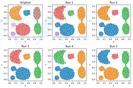
Figure A1.
Aggregation—Clusters from different runs, unique color/marker.
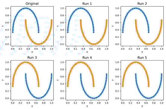
Figure A2.
Two Moons—Clusters from different runs, unique color/marker.
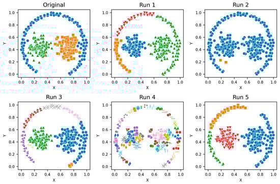
Figure A3.
Path-based—Clusters from different runs, unique color/marker.
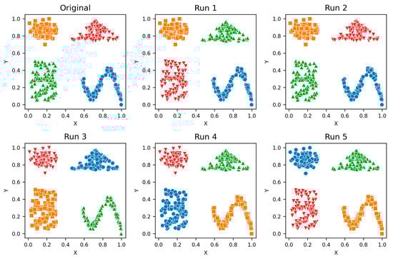
Figure A4.
Shapes—Clusters from different runs, unique color/marker.

Figure A5.
Spiral—Clusters from different runs, unique color/marker.
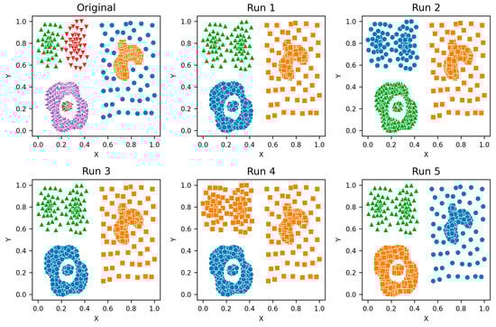
Figure A6.
Zahn’s Compound—Clusters from different runs, unique color/marker.
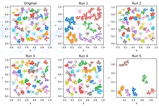
Figure A7.
S2—Clusters from different runs, unique color/marker.
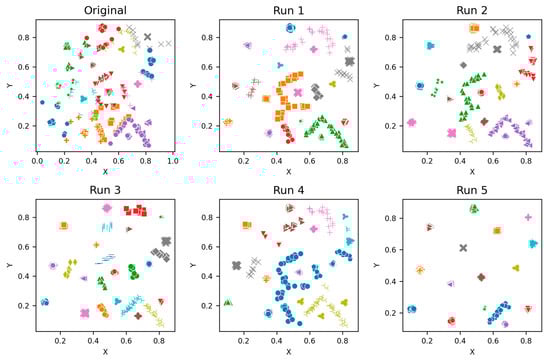
Figure A8.
A3—Clusters from different runs, unique color/marker.
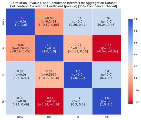
Figure A9.
Aggregation—Correlation of metrics. Color shows correlation strength; p-values indicate significance, and confidence intervals show range certainty.
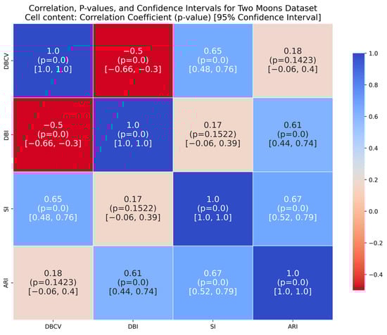
Figure A10.
Two Moons—Correlation of metrics. Color shows correlation strength; p-values indicate significance, and confidence intervals show range certainty.
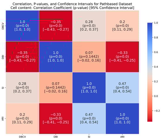
Figure A11.
Path-based—Correlation of metrics. Color shows correlation strength; p-values indicate significance, and confidence intervals show range certainty.
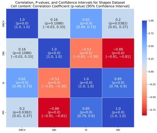
Figure A12.
Shapes—Correlation of metrics. Color shows correlation strength; p-values indicate significance, and confidence intervals show range certainty.
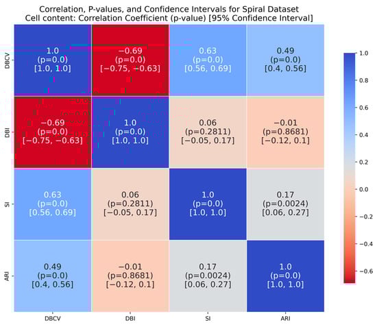
Figure A13.
Spiral—Correlation of metrics. Color shows correlation strength; p-values indicate significance, and confidence intervals show range certainty.
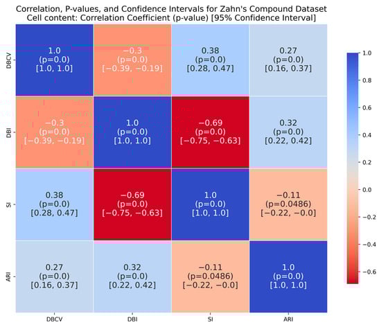
Figure A14.
Zahn’s Compound—Correlation of metrics. Color shows correlation strength; p-values indicate significance, and confidence intervals show range certainty.
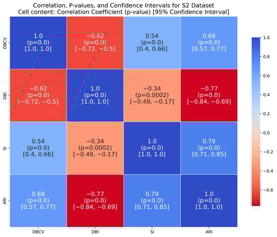
Figure A15.
S2—Correlation of metrics. Color shows correlation strength; p-values indicate significance, and confidence intervals show range certainty.
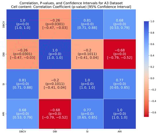
Figure A16.
A3—Correlation of metrics. Color shows correlation strength; p-values indicate significance, and confidence intervals show range certainty.
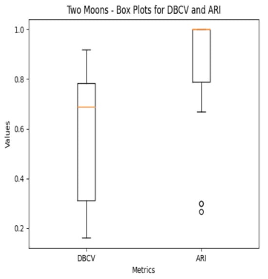
Figure A17.
Distribution of DBCV and ARI—Two Moons.
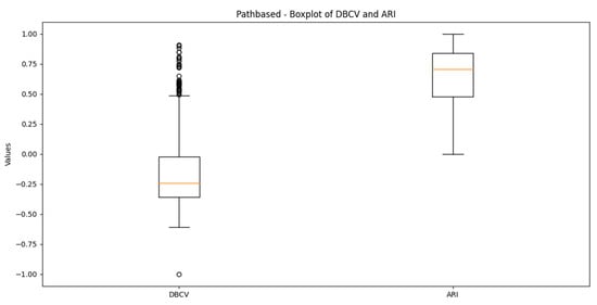
Figure A18.
Distribution of DBCV and ARI—Path-based.
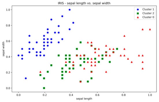
Figure A19.
IRIS—Sepal Length vs. Sepal Width.
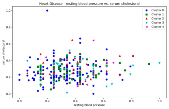
Figure A20.
Heart Disease—resting bp vs. cholesterol.
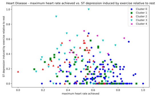
Figure A21.
Heart Disease—heart rate vs. depression.
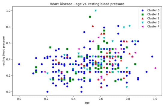
Figure A22.
Heart Disease—age vs. resting bp.
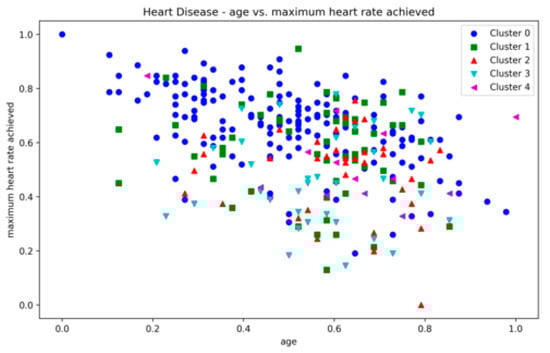
Figure A23.
Heart Disease—age vs. max. heart rate.
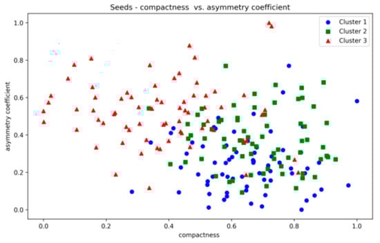
Figure A24.
Seeds—compactness vs. asymmetry.
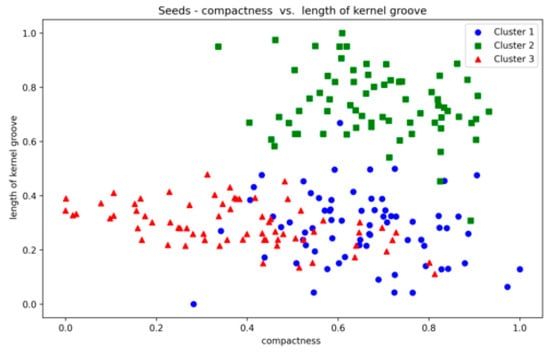
Figure A25.
Seeds—compactness vs. kernel groove.
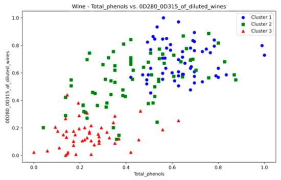
Figure A26.
Wine—total phenols vs. diluted wines.
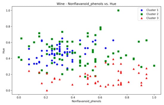
Figure A27.
Wine—nanoflavanoid vs. hue.
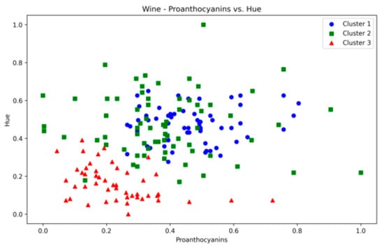
Figure A28.
Wine—proanthocyanins vs. hue.
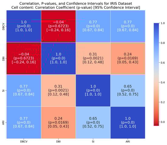
Figure A29.
IRIS—Correlation of metrics. Color shows correlation strength; p-values indicate significance, and confidence intervals show range certainty.
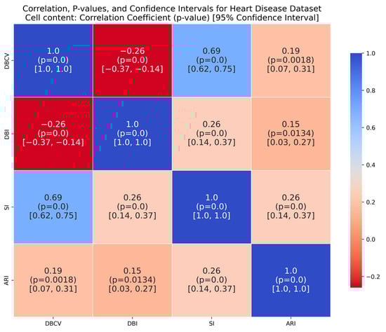
Figure A30.
Heart Disease—Correlation of metrics. Color shows correlation strength; p-values indicate significance, and confidence intervals show range certainty.
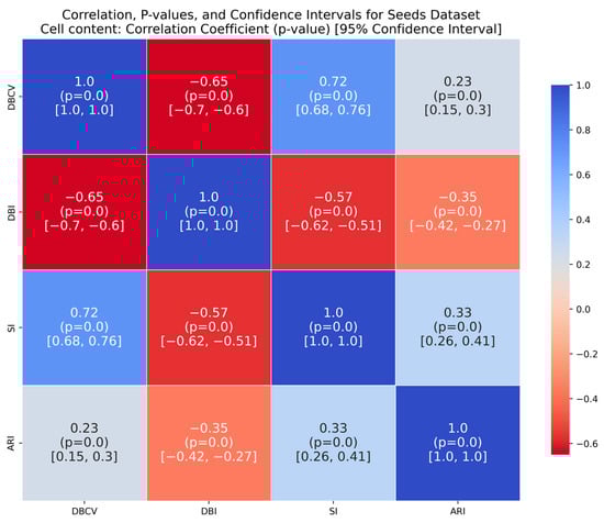
Figure A31.
Seeds—Correlation of metrics. Color shows correlation strength; p-values indicate significance, and confidence intervals show range certainty.
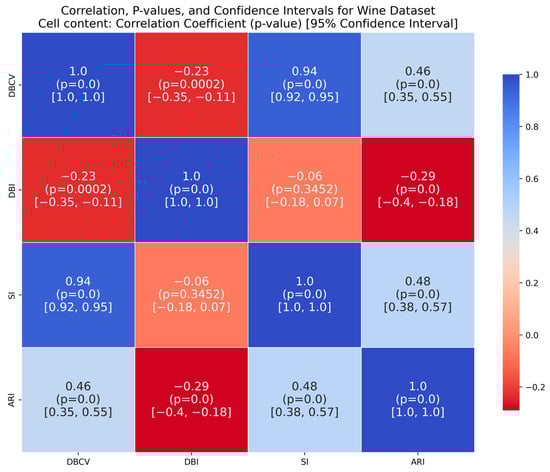
Figure A32.
Wine— Correlation of metrics. Color shows correlation strength; p-values indicate significance, and confidence intervals show range certainty.
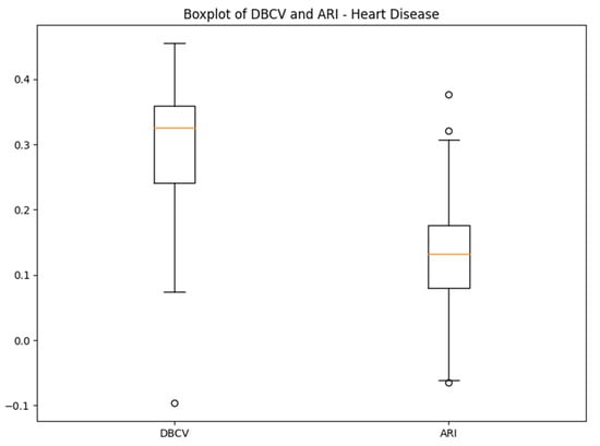
Figure A33.
Distribution of DBCV and ARI—Heart Disease.
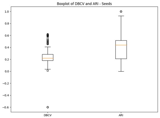
Figure A34.
Distribution of DBCV and ARI—Seeds.
Appendix B. Grid-Search for Parameters of the Original DENCLUE
For the original DENCLUE algorithm, a sufficiently large grid was defined spanning the parameter space. Specifically, Grid Search with Coarse–Fine Iterations was applied, which involves defining a range (grid) for the parameters and iteratively testing different combinations from the grid. The objective was to find the parameter values that produce the best clustering results in terms of the chosen clustering quality metrics.
Coarse Grid Search
First a coarse grid for the parameters was defined, which served as an initial step to quickly scan a wide range of parameter values. The coarse grid search space was defined as follows:
- σ ranges from 0 to 1, with a step size of 0.1;
- ξ ranges from 1 to the total number of data points (nPoints), with a step size of 10.
This initial search identified regions of interest for the parameters that showed promising results in terms of clustering quality, specifically the DBCV values and the cluster coverage.
Fine Grid Search
Once the initial regions of interest were identified, the fine grid search was applied. In this phase, a grid with narrower intervals was created around the identified regions of interest. The objective was to perform a more detailed exploration of these regions. The fine grid search involved:
- A finer grid for σ with a smaller step size, e.g., 0.01, centred around the promising σ values from the coarse search;
- Likewise, a finer grid for ξ with a smaller step size, e.g., 2, centred around the promising ξ values from the coarse search;
- The best results were manually selected based on the same objective crietria applied to the DE’s parameter optimisation, i.e., the DBCV and the Coverage. This ensured a fair comparison between the two approaches.
Initally, the coarse-grid search was applied and the promising regions were identified. For all datasets, the non-overlapping regions of interest were found and presented in Table A15. Subsequently, upon discovering the promising regions for σ and ξ, the fine grid search was applied. The results with the best DBCV and best Coverage are sepearetly identified and presented in Table A16 for real datasets and Table A17 for synthetic datasets. The clustering visualisations for synthetic datasets are shown in Figure A35.
The results clearly indicate that a pre-defined grid failed to identify true underlying structure across diverese datasets. The defined grid failed to identify any promising regions for Path-based and A3 datasets i.e., a single cluster was produced. Morever, even when the grid-search produced non-singular clusters, it deviated significantly from true clusters for datasets such as for Shapes, Spiral and S2. Clearly, there is a need for a more refined or tailored grid for each dataset for effective parameters searches. Additionally, the decision to select the best results further requires user intervention. Whereas the proposed method addresses these limitaions by: (1) automatically estimating DENCLUE parameters by exploiting DE’s capabilities; (2) the DE converges to the best result eliminating the need for manual verification by user.
Table A15.
Promising Regions from the Coarse-Grid Search.
Table A15.
Promising Regions from the Coarse-Grid Search.
| Dataset | σ (Range) | ξ (Range) | |
|---|---|---|---|
| Synthetic | Aggregation | {0.1} | {2–62} |
| Two Moons | {0.1–0.2, 0.2} | {2, 2–12} | |
| Path-based | {0.1} | {2–42} | |
| Shapes | {0.1–0.2, 0.2} | {2–42, 42–82} | |
| Spiral | {0.1} | {2–22} | |
| Zahn’s Compound | {0.1} | {2–42} | |
| S2 | {0.1} | {2–62} | |
| A3 | {0.1} | {2–42} | |
| Real | IRIS | {0.1, 0.2–0.4, 0.3–0.4} | {2, 2–22, 12–42} |
| Heart Disease | {0.1, 0.2, 0.3, 0.4–0.9, 0.6–0.9, 0.7–0.9, 0.9} | {2, 2,2, 2–12, 12–22, 22–32, 42} | |
| Seeds | {0.1–0.3, 0.2} | {2, 2–12} | |
| Wine | {0.2–0.6, 0.4–0.5, 0.5} | {2, 2–32, 42} |
Table A16.
Clustering Results Original DENCLUE vs. Proposed Method—Real Datasets.
Table A16.
Clustering Results Original DENCLUE vs. Proposed Method—Real Datasets.
| Dataset | Method & Criteria | σ | ξ | DBCV | Coverage | SI | DBI | ARI | Clusters |
|---|---|---|---|---|---|---|---|---|---|
| IRIS | OD—Best DBCV | 0.23 | 2 | 0.247 | 0.99 | 0.637 | 0.679 | 0.56 | 2 |
| OD—Best Coverage | 0.25 | 16 | 0.15 | 1.00 | 0.634 | 0.692 | 0.57 | 2 | |
| Proposed Method | 0.3905 | 34 | 0.150 | 1.00 | 0.633 | 0.692 | 0.568 | 2 | |
| Heart Disease | OD—Best DBCV | 0.1 | 2 | 0.620 | 0.05 | 0.833 | 0.724 | 0.02 | 8 |
| OD—Best Coverage | 0.89 | 2 | 0.062 | 0.96 | 0.321 | 1.555 | 0.11 | 22 | |
| Proposed Method | 0.7916 | 2 | 0.089 | 0.93 | 0.383 | 1.461 | 0.128 | 25 | |
| Seeds | OD—Best DBCV | 0.1 | 2 | 0.129 | 0.60 | 0.521 | 1.340 | 0.09 | 41 |
| OD—Best Coverage | 0.3 | 2 | −0.385 | 1.00 | 0.073 | 1.602 | 2.6 × 10⁻⁶ | 2 | |
| Proposed Method | 0.2443 | 2 | −0.037 | 0.96 | 0.120 | 1.232 | 4.8 × 10⁻⁴ | 2 | |
| Wine | OD—Best DBCV | 0.2 | 2 | 0.809 | 0.02 | 0.908 | 0.373 | 1.00 | 2 |
| OD—Best Coverage | 0.59 | 2 | −0.205 | 0.97 | 0.129 | 1.775 | −0.01 | 3 | |
| Proposed Method | 0.4969 | 13 | −0.192 | 0.87 | 0.348 | 1.643 | 0.494 | 2 |
Table A17.
Clustering Results Original DENCLUE vs. Proposed Method—Synthetic Datasets.
Table A17.
Clustering Results Original DENCLUE vs. Proposed Method—Synthetic Datasets.
| Dataset | Method & Criteria | σ | ξ | DBCV | Coverage | SI | DBI | ARI | Clusters |
|---|---|---|---|---|---|---|---|---|---|
| Aggregation | OD *—Best DBCV | 0.1 | 62 | −0.036 | 0.62 | 0.622 | 0.802 | 0.74 | 2 |
| OD—Best Coverage | 0.1 | 2 | −0.104 | 1.00 | 0.451 | 0.913 | 0.73 | 4 | |
| Proposed Method | 0.1099 | 38 | −0.104 | 1.00 | 0.451 | 0.913 | 0.73 | 4 | |
| Two Moons | OD—Best DBCV | 0.1 | 2 | 0.161 | 1.00 | 0.391 | 1.33 | 1.00 | 2 |
| OD—Best Coverage | 0.1 | 2 | 0.161 | 1.00 | 0.391 | 1.33 | 1.00 | 2 | |
| Proposed Method | 0.1439 | 7 | 0.160 | 1.00 | 0.391 | 1.33 | 1.00 | 2 | |
| Path-based | OD—Best DBCV ** | 0.1 | 2 | −1 | 1.00 | −1 | 1.8 × 10308 | 0 | 1 |
| OD—Best Coverage ** | 0.1 | 2 | −1 | 1.00 | −1 | 1.8 × 10308 | 0 | 1 | |
| Proposed Method | 0.0615 | 4 | −0.415 | 0.97 | 0.458 | 1.192 | 0.549 | 4 | |
| Shapes | OD—Best DBCV | 0.1 | 26 | 0.248 | 0.75 | 0.736 | 0.531 | 1.00 | 3 |
| OD—Best Coverage | 0.2 | 42 | 0.074 | 1.00 | 0.559 | 0.813 | 0.71 | 3 | |
| Proposed Method | 0.1865 | 3 | 0.227 | 1.00 | 0.701 | 0.585 | 1.00 | 4 | |
| Spiral | OD—Best DBCV | 0.1 | 18 | −0.118 | 0.78 | 0.056 | 7.740 | 0.86 | 4 |
| OD—Best Coverage | 0.1 | 10 | −0.446 | 1.00 | 0.024 | 9.223 | 0.58 | 2 | |
| Proposed Method | 0.0423 | 2 | −0.235 | 1.00 | 0.010 | 7.737 | 1.00 | 3 | |
| Zahn’s Compound | OD—Best DBCV | 0.1 | 28 | 0.212 | 0.75 | 0.713 | 0.580 | 0.75 | 2 |
| OD—Best Coverage | 0.1 | 4 | −0.095 | 1.00 | 0.576 | 0.823 | 0.76 | 4 | |
| Proposed Method | 0.1181 | 3 | −0.097 | 1.00 | 0.602 | 0.779 | 0.740 | 3 | |
| S2 | OD—Best DBCV | 0.1 | 18 | −0.268 | 0.99 | 0.035 | 0.137 | 0.892 | 3 |
| OD—Best Coverage | 0.1 | 18 | −0.268 | 0.99 | 0.035 | 0.137 | 0.892 | 3 | |
| Proposed Method | 0.025 | 19 | 0.906 | 0.86 | 0.975 | 0.938 | 0.282 | 16 | |
| A3 | OD—Best DBCV ** | 0.1 | 2 | −1 | 1.00 | −1 | 1.8 × 10308 | 0 | 1 |
| OD—Best Coverage ** | 0.1 | 2 | −1 | 1.00 | −1 | 1.8 × 10308 | 0 | 1 | |
| Proposed Method | 0.0216 | 5 | −0.071 | 0.98 | 0.948 | 0.620 | 0.761 | 51 |
* OD denotes Original DENCLUE. ** For Path-based and A3 datasets, the grid-search was only able to produce one cluster, the one spanning all data points (100% coverage) was chosen as the best solution. Also, the DBCV, SI are at negative extreme (−1) while DBI reaches maximum infinity (numeric overflow).
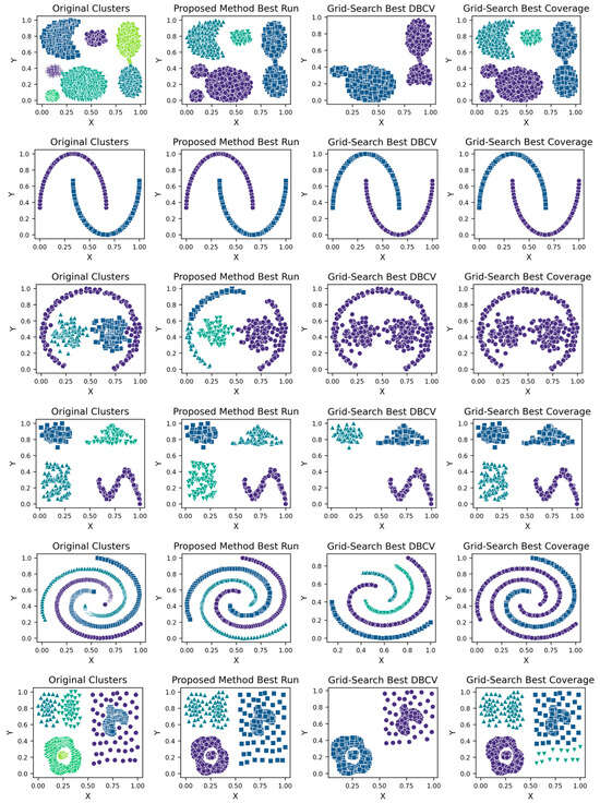
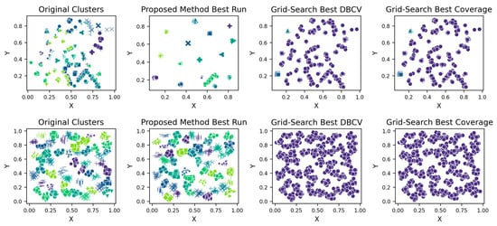
Figure A35.
Clustering Visualisations Proposed Method vs. Grid-Search on Original DENCLUE—Synthetic Datasets. From Top to Bottom: Aggregation, Moons, Path-based, Shapes, Spiral, Zahn’s Compound, S2 and A3. Each cluster is shown in a unique colour and marker.
References
- Gan, G.; Ma, C.; Wu, J. Data Clustering: Theory, Algorithms, and Applications, 2nd ed.; Society for Industrial and Applied Mathematics: Philadelphia, PA, USA, 2020; ISBN 978-1-61197-632-8. [Google Scholar]
- Rodriguez, M.Z.; Comin, C.H.; Casanova, D.; Bruno, O.M.; Amancio, D.R.; Costa, L.d.F.; Rodrigues, F.A. Clustering Algorithms: A comparative approach. PLoS ONE 2019, 14, e0210236. [Google Scholar] [CrossRef] [PubMed]
- Reddy, C.K.; Vinzamuri, B. A survey of partitional and hierarchical clustering algorithms. In Data Clustering; Chapman and Hall/CRC: Boca Raton, FL, USA, 2019; pp. 87–110. [Google Scholar] [CrossRef]
- Khan, K.; Rehman, S.U.; Aziz, K.; Fong, S.; Sarasvady, S.; Vishwa, A. DBSCAN: Past, present and future. In Proceedings of the 5th International Conference on the Applications of Digital Information and Web Technologies (ICADIWT 2014), Chennai, India, 17–19 February 2014; IEEE: Piscataway, NJ, USA, 2014; pp. 232–238. [Google Scholar] [CrossRef]
- Khader, M.; Al-Naymat, G. Discovery of arbitrary-shapes clusters using DENCLUE algorithm. Int. Arab J. Inf. Technol. 2020, 17, 629–634. [Google Scholar] [CrossRef] [PubMed]
- Ester, M.; Kriegel, H.-P.; Sander, J.; Xu, X. Density-based spatial clustering of applications with noise. In Proceedings of the International Conference Knowledge Discovery and Data Mining, Portland, OR, USA, 2–4 August 1996; Volume 240. [Google Scholar]
- Hinneburg, A.; Keim, D.A. An Efficient Approach to Clustering in Large Multimedia Databases with Noise; Bibliothek der Universität Konstanz: Konstanz, Germany, 1998; Volume 98. [Google Scholar]
- Ankerst, M.; Breunig, M.M.; Kriegel, H.P.; Sander, J. OPTICS: Ordering points to identify the clustering structure. SIGMOD Rec. ACM Spec. Interest Group Manag. Data 1999, 28, 49–60. [Google Scholar] [CrossRef]
- Ertöz, L.; Steinbach, M.; Kumar, V. Finding clusters of different sizes, shapes, and densities in noisy, high dimensional data. In Proceedings of the 2003 SIAM International Conference on Data Mining, San Francisco, CA, USA, 20 February 2003; pp. 47–58. [Google Scholar] [CrossRef]
- Mumtaz, K.; Duraiswamy, K. A novel density based improved k-means clustering algorithm–Dbkmeans. Int. J. Comput. Sci. Eng. 2010, 2, 213–218. [Google Scholar]
- Chaoji, V.; Hasan, M.A.; Salem, S.; Zaki, M.J. SPARCL: An effective and efficient algorithm for mining arbitrary shape-based clusters. Knowl. Inf. Syst. 2009, 21, 201–229. [Google Scholar] [CrossRef]
- Huang, H.; Gao, Y.; Chiew, K.; Chen, L.; He, Q. Towards effective and efficient mining of arbitrary shaped clusters. In Proceedings of the International Conference on Data Engineering, Chicago, IL, USA, 4 April 2014; pp. 28–39. [Google Scholar] [CrossRef]
- Kumar, K.M.; Reddy, A.R.M. A fast DBSCAN clustering algorithm by accelerating neighbor searching using groups method. Pattern Recognit. 2016, 58, 39–48. [Google Scholar] [CrossRef]
- Raykov, Y.P.; Boukouvalas, A.; Baig, F.; Little, M.A. What to do when K-means clustering fails: A simple yet principled alternative algorithm. PLoS ONE 2016, 11, e0162259. [Google Scholar] [CrossRef]
- Yu, D.; Liu, G.; Guo, M.; Liu, X.; Yao, S. Density peaks clustering based on weighted local density sequence and nearest neighbor assignment. IEEE Access 2019, 7, 34301–34317. [Google Scholar] [CrossRef]
- Bhattacharjee, P.; Mitra, P. A survey of density based clustering algorithms. Front. Comput. Sci. 2021, 15, 151308. [Google Scholar] [CrossRef]
- Khader, M.; Al-Naymat, G. Performance comparison of two algorithms for arbitrary shapes clustering. In Proceedings of the 2019 International Arab Conference on Information Technology (ACIT), Al Ain, United Arab Emirates, 3–5 December 2019; IEEE: Piscataway, NJ, USA, 2019; pp. 20–26. [Google Scholar]
- Soni, N. Aged (automatic generation of eps for dbscan). Int. J. Comput. Sci. Inf. Secur. 2016, 14, 536. [Google Scholar]
- Gan, W.; Li, D. Optimal choice of parameters for a density-based clustering algorithm. In Proceedings of the International Workshop on Rough Sets, Fuzzy Sets, Data Mining, and Granular-Soft Computing, Halifax, NS, Canada, 11–14 October 2013; Springer: Berlin/Heidelberg, Germany, 2003; pp. 603–606. [Google Scholar]
- Khader, M.S.; Al-Naymat, G. VDENCLUE: An enhanced variant of DENCLUE algorithm. In Intelligent Systems and Applications; Arai, K., Kapoor, S., Bhatia, R., Eds.; Advances in Intelligent Systems and Computing; Springer International Publishing: Cham, Switzerland, 2021; Volume 1251, pp. 425–436. ISBN 978-3-030-55186-5. [Google Scholar]
- Zhang, J.; Sanderson, A.C. JADE: Adaptive differential evolution with optional external archive. IEEE Trans. Evol. Comput. 2009, 13, 945–958. [Google Scholar] [CrossRef]
- Rahnamayan, S.; Tizhoosh, H.R.; Salama, M.M. Opposition-based differential evolution. IEEE Trans. Evol. Comput. 2008, 12, 64–79. [Google Scholar] [CrossRef]
- Das, S.; Abraham, A.; Chakraborty, U.K.; Konar, A. Differential evolution using a neighborhood-based mutation operator. IEEE Trans. Evol. Comput. 2009, 13, 526–553. [Google Scholar] [CrossRef]
- Khader, M.; Al-Naymat, G. An overview of various enhancements of denclue algorithm. In Proceedings of the ACM International Conference Proceeding Series, Phoenix, AZ, USA, 26–28 June 2019. [Google Scholar] [CrossRef]
- Yu, X.-G.; Jian, Y. A new clustering algorithm based on KNN and DENCLUE. In Proceedings of the 2005 International Conference on Machine Learning and Cybernetics, Guangzhou, China, 18–21 August 2005; IEEE: Piscataway, NJ, USA, 2005; Volume 4, pp. 2033–2038. [Google Scholar]
- Luo, Y.; Zhang, K.; Chai, Y.; Xiong, Y. Multi-parameter-setting based on data original distribution for denclue optimization. IEEE Access 2018, 6, 16704–16711. [Google Scholar] [CrossRef]
- Zhang, K.; Xiong, Y.; Huang, L.; Chai, Y. A novel algorithm based on avoid determining noise threshold in DENCLUE. In Proceedings of the 2016 Chinese Intelligent Systems Conference, Xiamen, China, 22 September 2016; Jia, Y., Du, J., Zhang, W., Li, H., Eds.; Lecture Notes in Electrical Engineering. Springer: Singapore, 2016; Volume 405, pp. 301–311, ISBN 978-981-10-2334-7. [Google Scholar]
- Jin, H.; Wang, S.; Zhou, Q.; Li, Y. Optimal bandwidth selection for density-based clustering. In Database Systems for Adanced Applications; Xu, J., Yu, G., Zhou, S., Unland, R., Eds.; Lecture Notes in Computer Science; Springer: Berlin/Heidelberg, Germany, 2011; Volume 6637, pp. 156–167. ISBN 978-3-642-20243-8. [Google Scholar]
- Conghua, X.I.E.; Chang, J.; Yuqing, S. Hill-down strategy based density clustering and its application to medical image data. In Proceedings of the 2nd International ICST Conference on Scalable Information Systems, Suzhou, China, 5–7 June 2007; 2010. [Google Scholar]
- Santosh, T.; Ramesh, D. DENCLUE-DE: Differential evolution based DENCLUE for scalable clustering in big data analysis. In Proceedings of the Second International Conference on Computer Networks and Communication Technologies, Kuala Lumpur, Malaysia, 12–24 August 2020; Smys, S., Senjyu, T., Lafata, P., Eds.; Lecture Notes on Data Engineering and Communications Technologies. Springer International Publishing: Cham, Switzerland, 2020; Volume 44, pp. 436–445, ISBN 978-3-030-37050-3. [Google Scholar]
- Hinneburg, A.; Gabriel, H.-H. DENCLUE 2.0: Fast clustering based on kernel density estimation. In Advances in Intelligent Data Analysis VII; Berthold, R.M., Shawe-Taylor, J., Lavrač, N., Eds.; Lecture Notes in Computer Science; Springer: Berlin/Heidelberg, Germany, 2007; Volume 4723, pp. 70–80. ISBN 978-3-540-74824-3. [Google Scholar]
- Storn, R.; Price, K. Differential evolution—a simple and efficient heuristic for global optimization over continuous spaces. J. Glob. Optim. 1997, 11, 341–359. [Google Scholar] [CrossRef]
- Pant, M.; Zaheer, H.; Garcia-Hernandez, L.; Abraham, A. Differential evolution: A review of more than two decades of research. Eng. Appl. Artif. Intell. 2020, 90, 103479. [Google Scholar]
- Zaharie, D. A comparative analysis of crossover variants in differential evolution. In Proceedings of the IMCSIT, Wisla, Poland, 15–17 October 2007; Volume 2007, pp. 171–181. [Google Scholar]
- Lampinen, J.; Zelinka, I. Mixed integer-discrete-continuous optimization by differential evolution. In Proceedings of the 5th International Conference on Soft Computing, Copenhagen, Denmark, 27–28 April 2024; Citeseer: Princeton, NJ, USA, 1999; Volume 71, p. 76. [Google Scholar]
- Hubert, L.; Arabie, P. Comparing partitions. J. Classif. 1985, 2, 193–218. [Google Scholar] [CrossRef]
- Rousseeuw, P.J. Silhouettes: A graphical aid to the interpretation and validation of cluster analysis. J. Comput. Appl. Math. 1987, 20, 53–65. [Google Scholar] [CrossRef]
- Davies, D.L.; Bouldin, D.W. A cluster separation measure. IEEE Trans. Pattern Anal. Mach. Intell. 1979, PAMI-1, 224–227. [Google Scholar] [CrossRef]
- Lei, Y.; Bezdek, J.C.; Romano, S.; Vinh, N.X.; Chan, J.; Bailey, J. Ground truth bias in external cluster validity indices. arXiv 2016, arXiv:1606.05596. [Google Scholar] [CrossRef]
- Liu, Y.; Li, Z.; Xiong, H.; Gao, X.; Wu, J. Understanding of Internal Clustering Validation Measures. In Proceedings of the 2010 IEEE International Conference on Data Mining, Sydney, Australia, 13–17 December 2010; IEEE: Piscataway, NJ, USA, 2010; pp. 911–916. [Google Scholar]
- Bertsimas, D.; Orfanoudaki, A.; Wiberg, H. Interpretable clustering: An optimization approach. Mach. Learn. 2021, 110, 89–138. [Google Scholar] [CrossRef]
- Alizade, M.; Kheni, R.; Price, S.; Sousa, B.C.; Cote, D.L.; Neamtu, R. A comparative study of clustering methods for nanoindentation mapping data. Integr. Mater. Manuf. Innov. 2024, 13, 526–540. [Google Scholar] [CrossRef]
- Amrulloh, K. Comparison between davies-bouldin index and silhouette coefficient evaluation methods in retail store sales transaction data clusterization using k-medoids algorithm. In Proceedings of the 3rd South American International Industrial Engineering and Operations Management Conference, Asuncion, Paraguay, 19–21 July 2022; pp. 1952–1961. [Google Scholar]
- Moulavi, D.; Jaskowiak, P.A.; Campello, R.J.G.B.; Zimek, A.; Sander, J. Density-based clustering validation. In Proceedings of the SIAM International Conference on Data Mining 2014 (SDM 2014), Philadelphia, PA, USA, 24–26 April 2014; Volume 2, pp. 839–847. [Google Scholar] [CrossRef]
- Deb, K. An efficient constraint handling method for genetic algorithms. Comput. Methods Appl. Mech. Eng. 2000, 186, 311–338. [Google Scholar] [CrossRef]
- Das, S.; Suganthan, P.N. Differential evolution: A survey of the state-of-the-art. IEEE Trans. Evol. Comput. 2010, 15, 4–31. [Google Scholar] [CrossRef]
- Fränti, P.; Sieranoja, S. K-means properties on six clustering benchmark datasets. Appl. Intell. 2018, 48, 4743–4759. [Google Scholar] [CrossRef]
- Liang, S.; Han, D.; Yang, Y. Cluster validity index for irregular clustering results. Appl. Soft Comput. 2020, 95, 106583. [Google Scholar] [CrossRef]
- Lee, S.-H.; Jeong, Y.-S.; Kim, J.-Y.; Jeong, M.K. A new clustering validity index for arbitrary shape of clusters. Pattern Recognit. Lett. 2018, 112, 263–269. [Google Scholar] [CrossRef]
- Şenol, A. VIASCKDE Index: A novel internal cluster validity index for arbitrary-shaped clusters based on the kernel density estimation. Comput. Intell. Neurosci. 2022, 2022, 4059302. [Google Scholar] [CrossRef]
- Kelly, M.; Longjohn, R.; Nottingham, K. The UCI Machine Learning Repository. Available online: https://archive.ics.uci.edu (accessed on 20 August 2024).
- Chang, D.-X.; Zhang, X.-D.; Zheng, C.-W.; Zhang, D.-M. A robust dynamic niching genetic algorithm with niche migration for automatic clustering problem. Pattern Recognit. 2010, 43, 1346–1360. [Google Scholar] [CrossRef]
- Guo, C.; Zang, Y. Clustering algorithm based on density function and nichePSO. J. Syst. Eng. Electron. 2012, 23, 445–452. [Google Scholar] [CrossRef]
- Storn, R.; Price, K. Minimizing the Real Functions of the ICEC’96 Contest by Differential Evolution. In Proceedings of the IEEE International Conference on Evolutionary Computation, Aichi, Japan, 20–22 May 1996; IEEE: Piscataway, NJ, USA, 1996; pp. 842–844. [Google Scholar]
- Ronkkonen, J.; Kukkonen, S.; Price, K.V. Real-parameter optimization with differential evolution. In Proceedings of the 2005 IEEE Congress on Evolutionary Computation, Edinburgh, UK, 2–5 September 2005; IEEE: Piscataway, NJ, USA, 2005; Volume 1, pp. 506–513. [Google Scholar]
- Zielinski, K.; Laur, R. Constrained single-objective optimization using differential evolution. In Proceedings of the 2006 IEEE International Conference on Evolutionary Computation, Vancouver, BC, Canada, 16–21 July 2006; IEEE: Piscataway, NJ, USA, 2006; pp. 223–230. [Google Scholar]
- Tavakkol, B.; Choi, J.; Jeong, M.K.; Albin, S.L. Object-based cluster validation with densities. Pattern Recognit. 2022, 121, 108223. [Google Scholar] [CrossRef]
- Sun, Y.; Ding, S.; Zhang, Z.; Jia, W. An improved grid search algorithm to optimize SVR for prediction. Soft Comput. 2021, 25, 5633–5644. [Google Scholar] [CrossRef]
- Feurer, M.; Hutter, F. Hyperparameter optimization. Autom. Mach. Learn. Methods Syst. Chall. 2019, 3–33. [Google Scholar] [CrossRef]
- Chowdhury, A.A.; Das, A.; Hoque, K.K.S.; Karmaker, D. A comparative study of hyperparameter optimization techniques for deep learning. In Proceedings of the International Joint Conference on Advances in Computational Intelligence: IJCACI 2021, Dhaka, Bangladesh, 23–24 October 2021; Springer: Berlin/Heidelberg, Germany, 2022; pp. 509–521. [Google Scholar]
- Hutter, F.; Kotthoff, L.; Vanschoren, J. Automated Machine Learning: Methods, Systems, Challenges; Springer Nature: Berlin/Heidelberg, Germany, 2019. [Google Scholar]
- Bergstra, J.; Bengio, Y. Random search for hyper-parameter optimization. J. Mach. Learn. Res. 2012, 13, 281–305. [Google Scholar]
- Ahmad, M.F.; Isa, N.A.M.; Lim, W.H.; Ang, K.M. Differential evolution: A recent review based on state-of-the-art works. Alex. Eng. J. 2022, 61, 3831–3872. [Google Scholar] [CrossRef]
- Hou, Y.; Wu, Y.; Liu, Z.; Han, H.; Wang, P. Dynamic multi-objective differential evolution algorithm based on the information of evolution progress. Sci. China Technol. Sci. 2021, 64, 1676–1689. [Google Scholar] [CrossRef]
- Zhou, Y.; Xiang, Y.; He, X. Constrained multiobjective optimization: Test problem construction and performance evaluations. IEEE Trans. Evol. Comput. 2020, 25, 172–186. [Google Scholar] [CrossRef]
- Xie, J.; Xiong, Z.-Y.; Dai, Q.-Z.; Wang, X.-X.; Zhang, Y.-F. A new internal index based on density core for clustering validation. Inf. Sci. 2020, 506, 346–365. [Google Scholar] [CrossRef]
Disclaimer/Publisher’s Note: The statements, opinions and data contained in all publications are solely those of the individual author(s) and contributor(s) and not of MDPI and/or the editor(s). MDPI and/or the editor(s) disclaim responsibility for any injury to people or property resulting from any ideas, methods, instructions or products referred to in the content. |
© 2024 by the authors. Licensee MDPI, Basel, Switzerland. This article is an open access article distributed under the terms and conditions of the Creative Commons Attribution (CC BY) license (https://creativecommons.org/licenses/by/4.0/).