Review

Graph Convolutional Network for Image Restoration: A Survey

1
School of Power and Energy, Northwestern Polytechnical University, Xi’an 710129, China
2
School of Physics, Maths and Computing, Computer Science and Software Engineering, The University of Western Australia, Perth 6009, Australia
3
National Maglev Transportation Engineering R&D Center, Tongji University, Shanghai 201804, China
4
School of Software, Northwestern Polytechnical University, Xi’an 710129, China
5
Yangtze River Delta Research Institute, Northwestern Polytechnical University, Taicang 215400, China
*
Author to whom correspondence should be addressed.
Mathematics 2024, 12(13), 2020; https://doi.org/10.3390/math12132020
Submission received: 1 May 2024 / Revised: 7 June 2024 / Accepted: 15 June 2024 / Published: 28 June 2024

Abstract

:
Image restoration technology is a crucial field in image processing and is extensively utilized across various domains. Recently, with advancements in graph convolutional network (GCN) technology, methods based on GCNs have increasingly been applied to image restoration, yielding impressive results. Despite these advancements, there is a gap in comprehensive research that consolidates various image denoising techniques. In this paper, we conduct a comparative study of image restoration techniques using GCNs. We begin by categorizing GCN methods into three primary application areas: image denoising, image super-resolution, and image deblurring. We then delve into the motivations and principles underlying various deep learning approaches. Subsequently, we provide both quantitative and qualitative comparisons of state-of-the-art methods using public denoising datasets. Finally, we discuss potential challenges and future directions, aiming to pave the way for further advancements in this domain. Our key findings include the identification of superior performance of GCN-based methods in capturing long-range dependencies and improving image quality across different restoration tasks, highlighting their potential for future research and applications.
MSC:
65D19

1. Introduction

Image restoration techniques have gained wide application across various fields, including computer science, medical fields [1,2], remote sensing [3,4], and security monitoring [5]. Image restoration is employed to address two primary types of degradation: (1) system-related degradations such as system aberrations leading to blur [6], atmospheric turbulence [7], motion artifacts [8], and diffraction effects [9]; (2) statistical degradations resulting from noise [10]. Several typical degraded images are shown in Figure 1 and Figure 2. Moreover, apart from images generated through advanced technologies, there is a growing need to digitize old images, particularly for cultural relic preservation. During the process of digitizing old images, there may be inherent degradation in the image itself or degradation caused by noise captured in the environment [11]. Image restoration aims to identify the underlying causes of image quality degradation and applies targeted restoration processes. Traditional image restoration methods primarily rely on probabilistic models and the acquisition of prior knowledge concerning image degradation. Establishing degradation models based on such prior knowledge serves as a prerequisite for these methods. With the increasing attention given to image restoration techniques, a plethora of image processing techniques have been proposed [12].
Currently, image restoration techniques can be categorized into three main categories: Filtering-Based Methods, Model-Based Methods, and Learning-Based Methods. Classical Filtering-Based Methods such as median filtering [13], Wiener filtering [14], Inverse filtering [15], Kalman filtering [16], and SVD pseudoinverse [17] employ artificially designed low-pass filters to eliminate image noise. Median filtering is effective for impulse noise, and it is simple to calculate but easy to cause blur. Wiener filtering can remove Gaussian noise and preserve details but depends on the statistical characteristics of noise. Inverse filtering can recover the image completely in theory, but it is sensitive to noise. Kalman filtering is suitable for dynamic image sequences to deal with time-dependent noise, but the calculation is complex. SVD pseudoinverse can deal with degraded images, but it is not robust to noise and easily amplifies noise. For images with similar blocks, noise removal can be achieved through non-local similar block stacking approaches, such as the classical non-local means (NLM) algorithm [18] and the block matching based 3D filtering (BM3D) algorithm [19]. Model-Based Methods for image restoration encompass nonlocal self-similarity (NSS) models [20], sparse models [21], gradient models [22], and Markov random field (MRF) models [23]. The NLM algorithm uses image self-similarity to effectively denoise but has high computational complexity. BM3D has a good effect by combining block matching and 3D transformation, but its hardware requirements are high. The NSS model uses non-local similarity to recover details but relies on prior knowledge. The sparse model needs to design a dictionary for denoising through sparse representation. The gradient model emphasizes that the gradient information preserves details but has high noise requirements. MRF models recover images based on statistical characteristics, but the optimization process is complex. While these Model-Based Methods boast strong mathematical foundations, they tend to exhibit degraded performance in recovering texture structures when confronted with heavy noise. Additionally, those methods often entail substantial time consumption due to the high complexity of iterative optimization. The advent of machine learning has brought about significant advancements in the field of image denoising [24]. Deep learning technology, in particular, has found widespread application in this domain.
Learning-Based Methods focus on learning potential mappings from noisy images to clean images and can be categorized into traditional learning-based methods and deep network-based learning methods [11]. In recent years, deep network-based methods have become mainstream methods due to their more promising denoising results than filter-based, model-based, and traditional learning-based methods. Zhang et al. [25] proposed a simple but effective denoising convolutional neural network (CNN) by superimposing convolutional, batch normalization, and corrected linear unit (ReLU) layers. Liu et al. [26] were inspired by the nonlocal similarity of images to propose a nonlocal recurrent network (NLRN), which is the first attempt to incorporate nonlocal operations into a recurrent neural network (RNN) for image recovery. DnCNN [27], FFDnet [28], and CBDnet [29] are proposed as a process of gradual generalization and gradual consideration of increasing the complexity of the noise. DnCNN mainly targets Gaussian noise for denoising, emphasizing the roles of residual learning and BN; FFDnet considers the generalization of the Gaussian noise into a more complex and real noise, and takes the noise level map as a part of the input to the network; CBDnet is mainly for the FFDnet, and starts with the noise level map part of the network, which is self-adaptively obtained by five-layer FCN to achieve a certain degree of blind denoising. DnCNN uses batch normalization and residual learning to accelerate the training process and improve the denoising performance, but FFDNet focuses on removing the more complex Gaussian noise with mainly different noise levels. Most of the denoising algorithms based on convolutional neural networks before FFDNet was proposed were specific to a particular kind of noise. In order to solve the problem of different noise levels, the authors of FFDNet utilized the noise level map as an input, which makes the network applicable to pictures with different noise levels. CBDNet consists of a noise estimation sub-network and a denoising sub-network [29], which are both composed of two parts, end to end training at the same time, and using signal independent noise based on the noise as well as the noise synthesized by the internal processing of the camera and the real noise picture joint training, to improve the generalization ability of the denoising network, but also to enhance the effect of the denoising. SRMD [30] is different from the previous three networks, mainly starting from the bicubic, taking into account the influence of the fuzzy kernel and the noise level, and combining LR, fuzzy kernel, and noise level uniformly in the input network to realize the recovery of different degradation models. SRMD can combine the degradation map and LR image together as the input of CNNs.
CNNs excel at extracting spatial features by utilizing weighted sums of center and neighboring pixels to generate feature maps. They are particularly effective at extracting spatial features from image or video data, where the pixels are organized in a structured matrix [31]. However, it is important to note that CNNs are well-suited for processing Euclidean data with regular grid structures and fixed positional relationships. Conversely, they exhibit poor performance when dealing with non-Euclidean data due to constraints related to their grid-like inputs, limitations of convolution operations, issues with data permutation and ordering, lack of translation invariance, and inability to handle complex topologies [32]. This limitation has led to the rise of GCNs [33] as a research focus. From a broader perspective, both GCNs and CNNs are methods of aggregating neighborhood information, but they operate on different types of data objects. The convolutional computations in CNNs are tailored towards fixed 2D raster structures found in graph data, while GCNs employ convolution to handle more general unstructured graph data. Additionally, both models exhibit local connectivity, which significantly reduces computational complexity compared to fully connected structures [34]. In terms of weight design, CNNs employ separate sets of weight parameters in their convolutional kernels to account for the fixed raster structure in image data. On the other hand, GCNs utilize a single set of weight parameters, allowing them to accommodate diverse graph data structures. Similar to CNNs, the convolutional kernel in GCNs operates on all points in the entire graph, and the weight parameters are shared across computations at each node. This parsimonious design reduces the number of parameters in the single-layer network and mitigates the risk of overfitting. As the number of convolutional layers increases, the receptive field of the model expands, encompassing larger perceptual domains.
Overall, while CNNs have demonstrated strong performance in processing image and video data, GCNs have revolutionized machine learning by extending convolutional operations to complex non-Euclidean data structures. The advantages of GCNs in handling graph data have opened up new avenues for research and applications, including social network analysis and drug discovery. As technology advances, hybrid models integrating CNNs and GCNs may emerge as a crucial direction for future research to fully harness the strengths of both approaches. While GCNs have proven highly effective in handling non-Euclidean data structures, their exploration in image processing remains largely untapped. Currently, there is a paucity of reviews on GCNs for image restoration. To address this gap, our aim is to provide an overview of the application of GCNs in image restoration, covering both practical applications and analytical insights. Additionally, we discuss state-of-the-art GCN methods for image restoration, explore avenues for further extension, highlight challenges for the future, and propose potential research directions. An overview of the survey is depicted in Figure 3.
The main contributions in this paper can be summarized as follows.
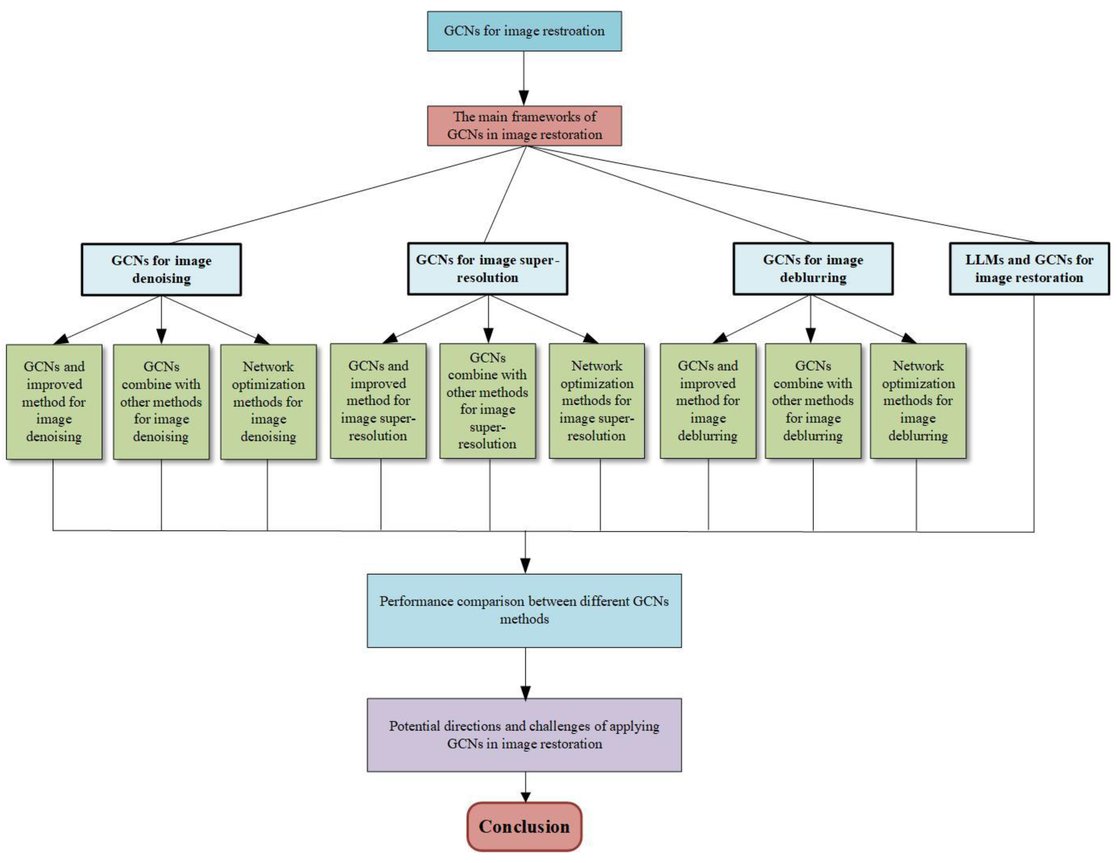
  • This overview provides an overview of several common methods of GCNs for image restoration.
  • This overview summarizes the solutions of GCNs in the field of image restoration (including image denoising, image super-resolution, image deblurring, LLMs, and GCNs for image restoration), and analyzes the motivation and principles of these methods in image restoration. Finally, we evaluate the graph restoration performance of these methods using both quantitative and qualitative analysis.
  • This overview points out some potential applications and challenges of GCNs in the field of image restoration.
Section 2 describes the development of GCNs and the current common GCN method introduction. Section 3 summarizes the methods of image restoration using GCNs from four aspects: image denoising, image super-resolution, image deblurring, and LLMs and GCNs for image restoration, as well as the analysis and comparison of these methods. Section 4 provides a performance comparison of these methods. Section 5 discusses potential research directions and challenges. Section 6 provides the conclusions.

2. Development of GCNs

Since CNNs, deep learning algorithms have achieved high performance in various tensor processing tasks in Euclidean space. For instance, face recognition algorithms [35] have reached an accuracy close to 100%, with more than 99% accuracy. However, in addition to the regular data in Euclidean space, there are a significant number of data in non-Euclidean space that possess a topological map structure, such as social network data and chemical structure data. These types of data cannot be effectively handled by traditional convolutional networks. To address the need for processing such topological structures, a novel algorithm called Graph Convolutional Neural Networks (GCNs) has been developed.

2.1. The Evolution of GCNs

Currently, the implementation of graph convolution can be categorized into two types:
  • Spectral domain graph convolution: This approach follows graph theory and the convolution theorem, transforming data to the spectral domain for processing and then back to the original domain. Working in the spectral domain is important because it leverages a robust mathematical framework based on the graph Laplacian and Fourier transform, which facilitates more precise and theoretically grounded operations [36]. Additionally, spectral methods capture global graph structure through eigenvalues and eigenvectors, enabling effective aggregation of information from distant nodes. This method is computationally efficient, as it involves element-wise products of Fourier transforms, reducing the number of parameters by defining filters in terms of eigenvalues. Spectral domain graph convolution is also adaptable to diverse graph topologies and scales, making it particularly useful for complex or dynamic graph structures.
  • Spatial domain graph convolution: This method defines the convolution operation directly in spatial space without relying on graph theory or the convolution theorem, offering greater flexibility. Spatial methods provide intuitive definitions and can be easily applied to a variety of graph structures without the need for spectral transformations.
The main models for spectral domain graph convolution are SCNN [33], ChebNet [37], and GCNs [38]. SCNN, proposed by Bruna et al. in 2014, generalizes CNNs to signals over general domains without translation group action but has drawbacks such as high computational cost, large parametric complexity, and inability to guarantee local links. To address these issues, Defferrard et al. proposed ChebNet in 2016, using Chebyshev polynomials for polynomial interpolation, significantly reducing time complexity. Kipf et al. [38] proposed the GCN model in 2016, simplifying ChebNet by only considering the first-order Chebyshev inequality, further reducing computational complexity. These advancements reflect ongoing efforts to optimize CNN principles for graph-structured data, balancing computational efficiency and the ability to capture intricate graph properties, thus expanding the applications and development of graph-based machine learning techniques.

2.2. The Fundamentals of GCNs

2.2.1. Graph Data

Graph data have become increasingly important in the development of machine learning and deep learning. While significant breakthroughs have been made in areas such as speech, image, and natural language processing, these data types are typically simple sequences or grid data [39], which are highly structured. Deep learning excels in processing this type of data. However, many real-world phenomena cannot be represented as sequences or grids, such as social networks, knowledge graphs, and complex file systems. These more complex structures need to be represented using graph data.
Consider a social network where each node represents a person, and each edge represents a friendship between two people. This network can be represented as Figure 4. Here, each person is a node, and the lines connecting them represent their friendships.
The simplest way to represent a graph structure is to use an adjacency matrix to capture the relationships between nodes and edges. For the above example, the adjacency matrix would look like Table 1.
In this matrix, a ‘1’ indicates a connection (friendship) between the nodes, and a ‘0’ indicates no connection.
Information in graph data is usually categorized into three levels:
Node information (V): Data about the nodes themselves (e.g., attributes of a person in a social network).
Edge information (E): Data about the connections between nodes (e.g., type or strength of friendship).
Overall graph information (U): Data about the graph as a whole (e.g., the average degree of nodes).
In this way, graph data effectively represent and process complex and unstructured data structures, expanding the application scope and capabilities of deep learning.

2.2.2. Principle of GCNs

The principle of GCNs revolves around extending traditional convolution operations to non-Euclidean data structures, specifically graphs. The primary goal of GCNs is to learn and leverage node features and topological structure in graph data for tasks such as node classification, link prediction, and graph classification [38].
In conventional Convolutional Neural Networks (CNNs), convolutions rely on the fixed grid structure of data (e.g., pixels in an image). However, in graph-structured data, connections between nodes are irregular and dynamically changing, lacking a fixed local neighborhood. Therefore, the key challenge for GCNs lies in designing a method that can perform feature propagation and aggregation across arbitrary graph structures.
The core aspects of GCNs’ principles include:
  • Laplacian Operator in Graphs:
Within the spectral graph convolution theory framework, GCNs can utilize the graph Laplacian matrix (often normalized) to capture topological relationships among nodes. The Laplacian matrix reflects the strength of connection between a node and its neighbors, and by performing eigen-decomposition on it, convolutions can be defined in the spectral domain of the graph.
2.
Message Passing Mechanism:
In practical GCN implementations, Kipf and Welling proposed a simplified approximation of spectral convolutions that employs a first-order neighborhood averaging approach for feature propagation. Each layer of the GCN aggregates neighboring node features through a transformed adjacency matrix and then applies a weight matrix for transformation.
This can be mathematically represented as:
H ( l + 1 ) = σ ( D ~ 1 2   A ~   D ~ 1 2   H ( L )   W ( l ) )
H ( L ) represents the node feature matrix at layer l ,
W ( l ) is the corresponding weight matrix,
A ~ = A + I N is the adjacency matrix A with added self-loops,
D ~ is the degree matrix of A ~ (diagonal elements equal to the sum of row or column entries plus one),
σ is an activation function like ReLU, which introduces non-linearity.
3.
Multilayer Perceptron (MLP)-like Architecture:
GCNs typically consist of multiple layers, each applying the message passing and feature transformation process. By stacking these layers, GCNs can learn increasingly abstract and higher-level node representations.
4.
Output Layers Tailored for Various Tasks:
For different tasks, the last layer of a GCN is designed accordingly. For instance, in node classification tasks, the output dimension of the last layer corresponds to the number of classes, and a softmax function provides the probability distribution over node classes; whereas, in graph-level classification, embeddings from all nodes might be pooled into a single vector, followed by fully connected layers and a softmax function to predict the graph’s class.
In summary, the principle of GCNs is to ingeniously adapt convolutional operations to graph-structured data, enabling the network to efficiently integrate both node attributes and their relative positions within the network, thus facilitating effective learning and representation of graph data. Its basic network framework is shown in Figure 5.

2.3. Common Models

Here are other basic graph neural network models.

2.3.1. Graph Sample and Aggregate (GraphSAGE)

GraphSAGE is a graph neural network model proposed by William L. Hamilton et al. [40] in 2017, specifically for node representation learning in large-scale graph datasets. Unlike earlier approaches like GCNs that rely on the entire graph structure for training, GraphSAGE allows for learning node embeddings incrementally by leveraging node feature information. This method significantly enhances the scalability of graph neural networks to large graphs.
The core principle of GraphSAGE is to learn how to aggregate feature information from a node’s local neighborhood while also preserving the node’s own features. Figure 6. shows how GraphSAGE clusters neighbor node information. This enables the generation of embeddings for nodes by sampling and aggregating features from their neighbors, rather than requiring the whole graph to be processed at once. Here is a breakdown of how GraphSAGE operates:
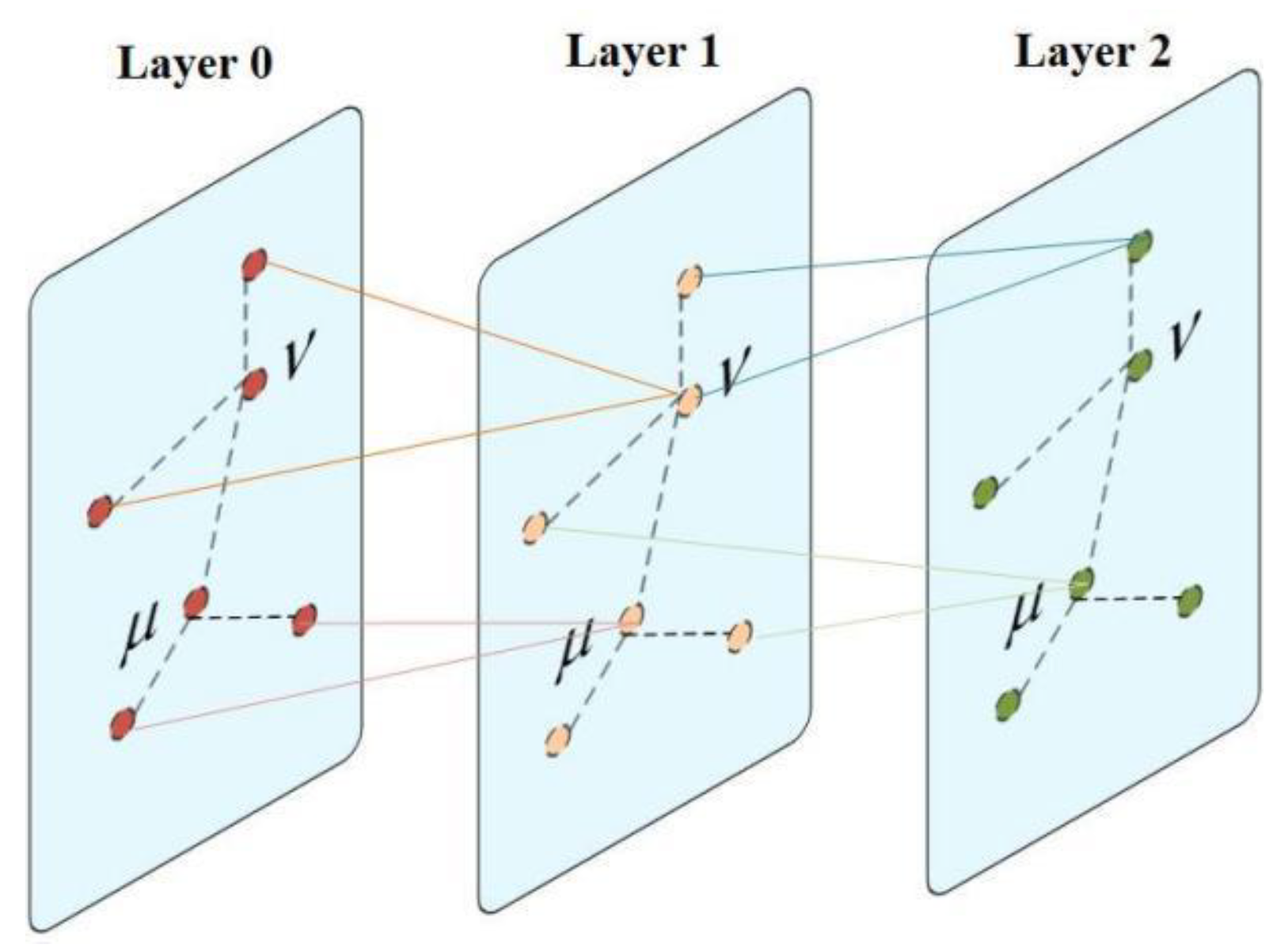
  • Sampling: The first step in GraphSAGE is to sample a fixed-size neighborhood for each node in the graph. Instead of using the entire neighborhood, GraphSAGE randomly selects a subset of neighbors at each depth of the neighborhood to consider. This sampling step is crucial for making the algorithm scalable and efficient.
  • Aggregation: Once the neighbors are sampled, GraphSAGE aggregates their features to generate a new feature vector for the target node. The aggregation function can be a simple mean of the neighbors’ features, a pooling operation (like max pooling), or even a more complex neural network that learns how to aggregate the features. The key idea is to create a summary of the neighborhood’s features that captures the local structural information.
  • Update: The aggregated feature vector is then combined with the target node’s current feature vector (e.g., through concatenation) and passed through a neural network layer (which can include non-linear activation functions) to generate the node’s new feature vector. This step effectively updates the node’s representation based on its own features and the aggregated features of its neighbors.
  • Normalization: Often, the new feature vector is normalized to ensure stable training dynamics. For example, L2 normalization can be applied to the resulting vector.
  • Repeat: Steps 1 through 4 can be repeated for multiple iterations or “layers”, allowing information to propagate from increasingly distant parts of the graph. With each iteration, the node representations incorporate information from a wider neighborhood.
  • Task-Specific Output: The final embeddings produced by GraphSAGE can be used for various downstream tasks such as node classification, link prediction, or even graph classification with the appropriate task-specific layers added on top of the GraphSAGE embeddings.
GraphSAGE’s novel approach to sampling and aggregation enables it to efficiently handle large-scale graphs. By focusing on local neighborhoods and using a fixed-size sampling strategy, it avoids the computational challenges associated with processing large graphs in their entirety. This makes GraphSAGE particularly well-suited for real-world applications where graphs can be very large and constantly evolving.

2.3.2. Graph Attention Networks (GATs)

GATs introduce an attention mechanism to the process of aggregating feature information from neighbors in a graph. This approach allows for more nuanced and dynamic weighting of neighbor contributions, as opposed to treating all neighbors equally or relying on predefined weights. The key innovation of GATs is their ability to assign different importance or weights to different nodes in a neighborhood, enabling the model to focus on more relevant information when updating a node’s representation. Figure 7 [41] shows this feature of GATs. Here are the core principles of how GATs work:
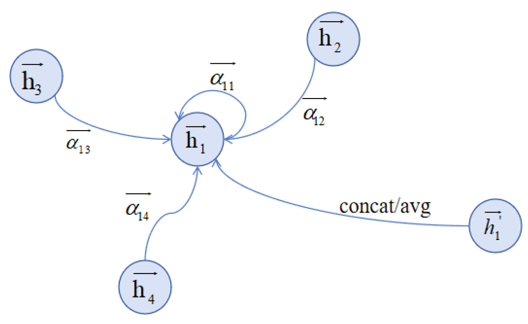
  • Node-Level Attention Mechanism: GATs leverage a self-attention strategy to compute attention coefficients that indicate the importance of each node’s features to another. This mechanism enables the model to dynamically prioritize information from different neighbors based on their feature similarity and relevance.
  • Feature Aggregation with Attention: For each node, the GAT model calculates the attention coefficients for all its neighbors. These coefficients are then used to weight the neighbors’ feature vectors before aggregation. The weighted sum of the neighbors’ features, scaled by the learned attention coefficients, forms the aggregated feature representation for the node. This process ensures that features from more relevant neighbors have a greater influence on the node’s new feature representation.
  • Multi-Head Attention for Stabilization: To stabilize the learning process and improve feature representation, GATs often employ multi-head attention. This involves running several independent attention mechanisms in parallel (each being a “head”), then concatenating or averaging their output feature representations. Multi-head attention allows the model to capture different aspects of feature relevance and provides a richer representation of the neighborhood’s features.
  • Non-linearity and Feature Transformation: Similar to other neural network approaches, GATs incorporate non-linear transformations into the feature aggregation process. Before computing attention coefficients, features can be transformed through a learnable linear transformation (e.g., a weight matrix). Non-linear activation functions (e.g., LeakyReLU) are also applied to the attention scores to introduce non-linearity into the model.
  • Normalization of Attention Coefficients: The attention coefficients for a node’s neighbors are normalized using a Softmax function, ensuring that they add up to one. This normalization step allows the model to effectively compare and contrast the importance of each neighbor within a local neighborhood context.
By dynamically weighting the contributions of neighbors based on the attention mechanism, GATs can effectively capture the relational information encoded in graphs. This approach is particularly beneficial for tasks like node classification, link prediction, and graph classification, where the relative importance of neighbors can significantly impact performance.

3. GCNs for Image Restoration

Image restoration is a crucial task in the field of computer vision, encompassing image denoising [41], image super-resolution [35], and image deblurring [42]. The primary objective of these tasks is to recover clear images from corrupted or low-quality ones. Graph Convolutional Networks (GCNs) have demonstrated significant potential in the domain of image restoration. GCNs, as a specialized type of neural network, conduct convolution operations on graph-structured data [39]. Given that an image can be conceptualized as a graph consisting of pixels (vertices) and their interconnections (edges), GCNs can be directly applied to various image processing tasks. In the context of image restoration, GCNs are capable of capturing long-range dependencies within the image while preserving its local structure. This unique capability enables GCNs to deliver exceptional performance when addressing complex challenges in the realm of image restoration.

3.1. GCNs for Image Denoising

In the realm of image denoising, GCNs have emerged as a prominent area of research due to their robust graph data processing capabilities. Unlike traditional convolutional neural networks, GCNs are adept at extracting features from non-Euclidean geometric structures, offering a novel approach for addressing image denoising tasks that involve intricate pixel relationships [38]. This subsection will provide a detailed overview of the recent advancements in GCN research pertaining to image denoising.

3.1.1. GCNs and Improved Methods for Image Denoising

Currently, GCNs are widely utilized across various domains for the purpose of image denoising. Researchers are employing GCNs along with advanced methods such as ECC and GATs to enhance the process of image denoising. Zhang et al. [43] introduced a label denoising (LDN) method based on GCNS and also proposed an innovative adaptive aggregate GCNs (AdarGCN) model for effectively reducing noise in image denoising tasks. AdarGCN demonstrates potential in enhancing the adaptive aggregation mechanism. However, these methods can suffer from high computational complexity, particularly in the adaptive aggregation process which requires significant resources for large-scale images. Li et al. [44] proposed an image denoising approach based on cross-patch consistency (CPNet). CPNet introduces a graph convolutional network known as Cross-Patch GCNs (CP-GCNs) to capture long-range context dependencies across patches. CP-GCNs effectively leverage cross-patch information through the construction of a cross-patch graph and the utilization of graph convolution operations to aggregate both local and non-local information. The cross-patch consistency approach can be computationally intensive due to the need to construct and process cross-patch graphs, limiting its applicability to real-time image processing tasks. Han [45] further enhances GCNs by proposing a graph embedding algorithm based on self-supervised graph denoising, aiming to enhance the robustness of graph neural networks.
The conventional GCN model typically treats all nodes’ features equally when processing images, whereas the graph attention network can dynamically adjust each node’s weight based on inter-node relationships and feature importance, thereby enhancing its ability to capture both local and global information in the image. Jiang et al. [42] proposed a graph attention denoising method called GAiA-Net. The proposed method captures both pixel-level and structure-level features through iterative transformation and learning, and aggregates between in-node (pixel-level) and out-node (structure-level) through information exchange and pooling. In this method, the graph attention mechanism is used to generate pixel-level attention and guide it to nodes with different distances to generate the final attention map. However, the iterative transformation and learning processes required to capture both pixel-level and structure-level features can lead to longer training times and higher computational demands. Based on the graph attention mechanism, Mou et al. [46] propose a graph attention network based image restoration method (GATIR), which achieves state-of-the-art performance on Mosaic and compression artifact reduction tasks by establishing feature-block-based non-local attention and utilizing graph convolution for selective feature aggregation. In order to adaptively balance image content and obtain better image denoising performance, Mou et al. [47] proposed a dynamic attention graph learning model (DAGL) for image restoration task. The model’s complexity increases significantly with the dynamic attention mechanism, potentially leading to slower inference times and higher memory usage. Liu et al. [48] used an edge enhancement module and a windowed graph attention convolutional network (WGAT) to solve the problem of denoising low-dose CT images. The edge enhancement module provides enough edge information for the encoder part at each stage, and WGAT combines the static and dynamic attention modules to explore the non-local self-similarity of the encoder, bottleneck, and decoder part of the LDCT image, which improves the denoising efficiency of the LDCT image. The edge enhancement module, while improving detail preservation, can introduce artifacts if not properly balanced, and the windowed attention mechanism can be computationally expensive.
Graph convolutional neural networks have been widely used in grid or point cloud image restoration tasks due to their adaptability to irregular structures, effective capture of local and global information, efficient processing of large-scale data, and flexibility and generalization. For example, Shen et al. [49] and Armando et al. [50] proposed a 3D mesh denoising method based on GCNs, which is able to remove noise and preserve geometric features when dealing with damaged 3D meshes. These methods require a high level of expertise to accurately design and implement, and may not be as effective on 2D image data without significant modifications. Traditional mesh denoising methods require manual feature design and can usually only perform local denoising. In contrast, the method using GCNs directly operates on the topology of the mesh through an end-to-end learning strategy, and can learn more meaningful features.
To address the over-smoothing problem of GCNs in image processing, Mostafa et al. [51] proposed a graph convolutional neural network called Permutohedral-GCNs, which has a global attention mechanism and is able to effectively classify and embed nodes in the graph. The global attention mechanism is implemented by an approximate Gaussian filtering method, which is computationally efficient and scalable. It avoids the inherent limited aggregation range of GCNs and allows nodes to aggregate features from different nodes, thus alleviating the over-smoothing phenomenon. Tian et al. [52] proposed a perceptual self-supervised learning network (PSLNet) for noisy image watermarking removal, which relies on a parallel network to remove the noise and the watermark. This method is very effective in removing noisy image watermarking compared to the popular convolutional neural network (CNN).
Table 2 provides an overview about GCNs as well as the improved method for image denoising.

3.1.2. GCNs Combine with Other Methods for Image Denoising

The application of graph convolutional networks (GCNs) combined with other methods in denoising is a powerful strategy. The ability of GCNs to model global context information and non-local self-similarity information is combined with the local spatial pattern extraction ability of convolutional neural networks (CNNs) or the noise distribution learning ability of generative adversarial networks (GANs), so as to achieve a more accurate and effective image denoising effect. This combination not only gives full play to the advantages of the respective models, such as the global information processing ability of GCNs and the local detail capture ability of CNNs, but also adapts to different types of data and noise patterns by designing specialized architectures. Fu et al. [56] proposed a method combining GCNs and CNNs to model the global relationship between pixels and channels. Chen et al.’s [57] method explores the non-local self-similarity of low-dose CT images through GCNs. This method uses a GAN to learn the noise distribution and construct the data, and then uses graph convolution (GCL) to explore the non-local self-similarity information of LDCT images, achieving better denoising results. Additionally, the CEGCN framework proposed by Liu et al. [58] fuses CNNs and GCNs to process hyperspectral images. These methods not only improve the denoising performance, but also enhance the adaptability of the network to complex noise distribution and image characteristics, showing the great potential and diversified application of GCNs combined with other methods in denoising technology. Table 3 shows the application of GCNs combined with other methods for denoising.

3.1.3. Network Optimization Methods for Image Denoising

Through the continuous optimization and innovation of GCNs, recent research results have demonstrated their significant application advantages in the field of denoising. Tian et al. [59] proposed a cross-transformer denoising CNN (CTNet) based on serial block (SB), parallel block (PB), and residual block (RB) to obtain clean images of complex scenes. The proposed method uses the enhanced residual structure depth to search for structural information for image denoising. In addition, to improve the denoising performance, CTNet embedded the transformer mechanism into SB and PB to extract complementary salient features, so as to effectively remove noise based on pixel relationships. The Adaptive Graph Prior Network (AGPNet) proposed by Jiang et al. [60] effectively captures the long-distance dependencies at the pixel and patch level through a novel graph construction method and k-nearest neighbor algorithm, realizes the exchange and integration of information at different levels, and breaks through the limitations of traditional denoising methods in dealing with complex dependencies. The PDE-GCN method proposed by Eliasof et al. [61] solves the problem of over-smoothing of deep networks by combining graph neural networks with partial differential equations, providing a more flexible architectural design that enhances the generalization ability and denoising efficiency of the model. Hattori et al. [62] proposed a self-prior learning method based on dual graph convolutional networks, which showed superior performance in mesh denoising by focusing on filtering vertex positions and normal vectors and avoiding the dependence on large-scale datasets. Fu et al.’s [63] dual-graph convolutional network has made innovations in the field of single image rain removal. By constructing two graphs to model and reason about the global relationship, it shows the powerful ability of GCNs to deal with global spatial and inter-channel relationships. These optimizations and innovations not only improve the performance of denoising techniques, but also extend the applicable scope of GCNs in denoising applications. By carefully optimizing the GCN, such as improving the graph construction method, combining partial differential equations, and introducing the self-prior learning mechanism, researchers can more deeply explore the internal structure and complex dependencies of the image, so as to achieve more accurate and efficient denoising effects. These results not only verify the great potential of GCNs in the field of image processing, but also provide new ideas and directions for future research. Table 4 presents an overview of this section.

3.2. GCNs for Image Super-Resolution

In the field of image super-resolution, the method based on deep learning has become an advanced technology to realize image enhancement. Image super-resolution technology aims to restore high-resolution images from low-resolution images, using a variety of deep learning models, such as convolutional neural networks (CNNs) and graph convolutional networks (GCNs), to enhance the details in the image and minimize distortion. Traditional CNN methods have achieved some success in the field of super-resolution, but may not be adequate in image feature representation due to their inherent limitations, such as their weak ability to handle non-Euclidean data. To overcome these problems, GCNs have gradually attracted attention as an effective deep learning tool.

3.2.1. GCNs and Improved Methods for Image Super-Resolution

In recent years, GCNs have been widely used in image and point cloud super-resolution tasks because of their powerful ability to capture the global relationship between image and point cloud data. Various GCN-based methods have been proposed by different research groups to improve the super-resolution performance (Table 5). For example, the CASGCN method proposed by Yang et al. [64] effectively captures the channel and spatial information of the image by combining channel attention and spatial graph convolution, and significantly improves the super-resolution performance. However, Yan et al.’s [65] SRGAT method, which uses a Graph Attention Network (GAT) to optimize single image super-resolution, shows excellent performance on multiple datasets. In the same year, Yang et al. [66] also introduced a method called Spatial Graph Convolutional Network (SGCN), which captured the global features of an image through a deep or wide network structure, and further enhanced the feature representation through the Residual Feature Refinement Module (RFRM) and Spatial Graph Attention (SGA).
In 2024, Yang et al. [75] proposed the “relation-Consistent Graph Convolutional Network” (RGCN), which not only uses GCNs to capture global image features, but also introduces a new spatial graph attention mechanism to further improve the performance of image super-resolution. In addition, other studies such as Zhang et al.’s [67] SERAN method, Wu et al.’s [68] AR-GCNs method, Chen et al.’s [69] GCNs-MA method, and Liang et al.’s [70] MAGSR method, etc., have demonstrated the strong application potential of GCNs in image and point cloud super-resolution tasks. These studies not only prove the effectiveness of GCNs in capturing the global relationship between image and point cloud data, but also show that the super-resolution performance can be further improved by different attention mechanisms and network structure improvements. These applications of GCNs have achieved good performance on multiple datasets and scale factors, which proves their wide applicability and promise in the field of image super-resolution. Table 5 presents an overview of this section.

3.2.2. GCNs Combine with Other Methods for Image Super-Resolution

The application of graph convolutional network (GCNs) in image processing tasks is increasing, and significant progress has been made especially in the fields of Image Super-Resolution (ISR) and Image Deblurring (Table 6). These studies make full use of the advantages of GCNs in processing spatial context information and non-local dependencies in images, and combine with traditional convolutional neural networks (CNNS) and other techniques to form efficient and innovative solutions. The CRAN (Context-inferring Attention Convolutional Network) proposed by Zhang et al. [76] is a breakthrough example. It effectively handles the image super-resolution task through the steps of context information extraction, context descriptor relationship inference, and context-inferring attention convolution. The CRAN network uses GCNs to extract and process the context information in an image, and then uses a CNN for feature extraction and convolution operations. This combination not only improves the resolution of the image, but also enhances the details and textures of the image, showing the powerful ability of GCNs in understanding and processing the image context. Tian et al. [77] proposed a dynamic network for image super-resolution (DSRNet), which consists of a residual enhancement block, a wide enhancement block, a feature refinement block, and a structure block. Experimental results show that the proposed method is competitive in terms of performance, time, and complexity of image super-resolution restoration. Liu et al. [58] focused on hyperspectral image (HSI) classification and proposed CEGCN (CNN-enhanced GCNs), a heterogeneous deep network that combines the advantages of CNNs and GCNs to perform feature learning on small-scale regular regions and large-scale irregular regions, respectively. This method can generate complementary spectral-spatial features, and at the same time solve the problem of data representation structure incompatibility between CNNs and GCNs through a graph encoder and decoder, so that the two networks can cooperate in a single network, which improves the accuracy and efficiency of HSI classification. Furthermore, Liu et al. [78] proposed RAN (Region-Aware Network) to solve the remote sensing image super-resolution problem, which adopts a contrastive learning strategy to capture potentially degraded representations and improves the quality of reconstructed images through the designed RAM (Region-Aware Module) module. The RAM module contains a 3D attention module for modeling channel and spatial information, and a GCN-based cross-patch feature aggregation module for exploring non-local information. This region-aware strategy and the design of high-level modules enable RAN to improve the image super-resolution performance while preserving texture details.
The study by Zhang et al. [81] combines GCNs with Graph Inference Attention Network (GRAN) to propose a lightweight solution to the electron microscopy image deblurring problem. By constructing a fully connected graph and treating the feature points as nodes in the graph and using GCNs for inference, this method can effectively capture the non-local relationships in the image and improve the deblurring performance. By applying GCNs to each node in the feature map and multiplying the response with the input feature map, the resulting enhanced visual component is crucial for improving the image quality. These studies demonstrate the potential of GCNs in image super-resolution and deblurring tasks, and provide new perspectives and methods for processing complex spatial relationships and contextual information in images by combining with traditional techniques such as CNNs.

3.2.3. Network Optimization Methods for Image Super-Resolution

Through continuous optimization and innovation of GCNs, recent research results show their significant application advantages in the field of image super-resolution (Table 7). A study by Xu et al. [82] proposed a method for applying GCNs to image deblurring and super-resolution tasks by transforming feature maps into graph nodes and using graph convolution for feature synthesis. By implicitly applying graph Laplacian regularization, this approach optimizes the structure of the feature map and thus achieves significant performance gains in image restoration tasks. Aiming at the high computational cost of Transformer on single image super-resolution task, Zhang et al. [83] proposed the Super Token Interaction Network (SPIN), which enhances the interpretability and efficiency of the model through superpixel clustering and attention mechanism. Li et al. [84] introduced the diffusion-based SRDiff model, which is the first attempt to use a diffusion probabilistic model for single image super-resolution reconstruction, by introducing residual prediction to speed up convergence. Liu et al.’s [85] research improves the performance of facial expression inpainting by improving Graph Convolutional Network (IGCN) and Region Relation building Module (RRMB). Yue et al. [86] used GCNs to solve the global spatial-temporal feature refinement problem in video super-resolution, demonstrating the strong potential of GCNs in video content analysis. These studies demonstrate the importance and effectiveness of GCNs and their optimization methods in improving the performance in image super-resolution, deblurring, and video processing tasks. Through these innovative approaches, researchers are able to address challenges such as high computational cost, low efficiency, and lack of interpretability, opening new avenues for future image processing techniques.

3.3. GCNs for Image Deblurring

In the field of deep learning, GCN-based image deblurring methods have made significant progress. As an effective method for processing graph structure data, GCNs have been widely used to deal with complex structural relationships in images. Since blurred images often contain distorted structural information, GCNs are used to restore the structural details in the image and improve the deblurring effect due to their unique neighborhood aggregation mechanism.

3.3.1. GCNs and Improved Methods for Image Deblurring

In the specific problem of using GCNs or related techniques to solve image deblurring, Liao et al. [87] propose RAAD-Net, an image deblurring network with two stages of coarse deblurring and fine deblurring to identify and remove different types of image blur. It uses the attention mechanism to identify the remaining blurred regions in the image, and adopts Graph Convolutional Networks (GCNs) to model these regions, so as to remove the blur more effectively. Tests on GoPro and HIDE datasets show that RAID-Net outperforms other existing deblurring methods. A study by Chen et al. [88] introduces a cloud removal method based on synthetic aperture radar (SAR), optical data fusion, and a graph-based feature aggregation network. Through the residual module, graph attention network, and graph-based feature aggregation mechanism, this method is able to effectively remove clouds from optical images. The proposed method outperforms other cloud removal methods on both simulated and real data. The work by Shen et al. [89] introduces the application of GCNs in remote sensing data processing, including image denoising, texture restoration, and image fusion, among others. GCNs can capture non-local, self-similar patterns; are suitable for processing multi-modal data such as optical, infrared, SAR, and lidar data; and are able to recover more detailed texture information. However, there are efficiency differences and iterative optimization challenges between GCNs and CNNs when the structured data are graphs. The DRTL method by Li et al. [90] is a method for real-world image super-resolution. By constructing a model called “Distortion Relation Network” (DRN), the correlation relationship between different distortion types is used to solve the problem of image super-resolution. The transfer of pre-trained task knowledge to the target distortion type super-resolution task is realized. Experimental results show that this method performs well on real-world image super-resolution tasks. These studies demonstrate diverse applications of GCNs and related techniques in the field of image processing, including solutions to problems such as deblurring, cloud removal, data fusion, denoising, texture restoration, and image super-resolution. Table 8 gives an overview of this part.

3.3.2. GCNs Combine with Other Methods for Image Deblurring

In recent years, there have been few studies on combining GCNs with other methods for image deblurring. Li et al. [91] proposed a deblurring method based on wavelet transform, iterative filter adaptive module, and graph convolutional network to solve the out-of-focus blur problem of images. By predicting an adaptive deblurring filter for each pixel, the proposed method improves the image restoration performance while keeping the computational cost low. Experimental results show that the proposed method can produce images with better visual quality and stronger robustness in various scenarios. In addition, Zhang et al. [81] proposed a lightweight graph inference attention network (GRAN) for image deblurring of low quality (LQ) microscope images. This method used GCNs to capture the non-local relationship between input feature points, and introduced a graph inference attention block (GRAB) in GRAN to solve the problem of over-smoothing of the network, which could be easily inserted into other networks. Experimental results show that GRAN outperforms other state-of-the-art deblurring techniques on electron microscopy (EM) and histology (HIST) datasets. Table 9 gives an overview of this section.

3.3.3. Network Optimization Methods for Image Deblurring

In recent years, the GCN method has been innovated for image deblurring, and there are several research works as follows. Liu et al. [85] proposed a facial expression inpainting method based on an improved Graph Convolutional Network (IGCN) to model the relationships of facial regions, and process facial patches through a Region Relationship Building Module (RRMB) and IGCN to optimize feature extraction. Eliasof et al. [61] introduced PDE-GCNs, a partial differential equation-based graph neural network architecture to improve the efficiency and theoretical nature of graph network processing. Although it mainly addresses the problem of over-smoothing, it is potentially applicable to image deblurring tasks as well. Table 10 gives an overview of this section.

3.4. Integration of Large Language Models (LLMs) and GCNs for Image Restoration

Recent advancements in artificial intelligence have seen the rise of LLMs, such as GPT-3 and BERT, which excel in natural language processing tasks due to their ability to capture complex dependencies and contextual information. Integrating LLMs with GCNs presents a promising approach for enhancing image restoration tasks.

3.4.1. Synergistic Capabilities

LLMs can contribute to image restoration in several ways:
  • Contextual Understanding: LLMs are adept at understanding and generating complex contextual information [92]. When integrated with GCNs, LLMs can help interpret high-level contextual information about the image content, which can be used to guide the restoration process more effectively.
  • Multi-Modal Learning: LLMs can facilitate multi-modal learning by bridging the gap between textual and visual data [93]. By incorporating textual descriptions or annotations associated with images, LLMs can provide additional context that GCNs can leverage to improve restoration accuracy.
  • Feature Extraction: LLMs can be utilized to extract semantic features from textual data that can complement the structural features extracted by GCNs from image data [94]. This complementary feature set can enhance the overall performance of image restoration models.

3.4.2. LLMs for Image Restoration

Traditional image restoration tasks are often designed for specific types, are difficult to generalize to handle diverse degraded or unknown scenes, and lack interactivity with users, limiting their applicability and flexibility [95,96] (Table 11).
Jin et al. [95] proposed LLMRA (Multimodal Large Language Model-Based Image Restoration Assistant) using pre-trained multimodal language models such as IDEFICS to generate image degradation text descriptions, encoded by CLIP, and degraded through Context Enhancement Module (CEM). Context-based Transformer (DC-former) integrates these contexts into the restoration network to achieve more accurate and tunable image restoration. The Clarity ChatGPT system proposed by Wei et al. [96] is an interactive image processing system that combines ChatGPT’s conversational intelligence and multiple image restoration and enhancement methods to automatically detect degradation types, select appropriate methods, and iteratively generate satisfactory results based on user feedback. System features include CLIP-driven degradation classification, reference-free quality assessment, region-specific processing, and advanced fusion technology. With rich common sense, powerful semantic understanding, and generation capabilities, LLMs have been explored for use in image processing to enhance feature extraction and understand the degraded information of images. They can generate text to describe image attributes, capture low-level features, and assist image understanding, thereby improving restoration accuracy and adjustability. LLMs can also be used directly as predictors, or, by combining them with GCNs, to improve tasks such as node classification [94]. In text attribute graphs, LLMs are combined with GCNs to enhance node features by generating text descriptions, improving graph feature representation, and solving the problems of label data scarcity and heterogeneous graphs. LLMs are combined with knowledge graphs to enhance the model’s reasoning capabilities and reduce illusions, improving understanding of complex data, such as scene graphs guiding robot task planning and drug recommendation [97].

4. Experimental Results

4.1. Datasets

4.1.1. Training Datasets

  • Image denoising training datasets
In the field of image denoising, researchers have extensively used real and synthetic datasets such as BSD500 [98,99], Urban100 [100], Set12 [42,101], SIDD [102], DIV2K [103], CBSD68 [60,104], Rain100L/H [105], Rain800 [106], etc., which contain different levels of noise, such as Gaussian noise, actual camera noise, raindrop noise, etc., and provide noise-free clean images as ground truth. For 3D grid denoising, 3D grid model datasets scanned from Microsoft Kinect devices [53], real scan data downloaded from academic repositories [50], and self-built simulated noise datasets have been used. In the study of low-dose CT image denoising, datasets from clinical cases and challenges, such as NIH AAPM-Mayo Clinic Low-Dose CT Grand Challenge [57], have been used.
2.
Image super-resolution training datasets
For super-resolution of natural images and videos, the benchmark datasets used are Set5 [107], Set14 [108], B100 [82], Urban100, and Manga109 [109]. These datasets are used to evaluate the performance of super-resolution algorithms at different magnification factors and are compared by quantitative indicators such as peak signal-to-noise ratio (PSNR) and structural similarity index (SSIM). In the field of medical image super-resolution (MedSR), the DIV2K dataset is widely used as a training resource. The dataset contains high-quality natural scene images and can provide rich training materials for medical images. For hyperspectral image super-resolution, researchers have used datasets such as CAVE [110], NUS [111], and NTIRE2018 [112], which contain images with a variety of waveband information and can be used to evaluate the effect of hyperspectral image super-resolution technology. In the field of point cloud data super-resolution, two datasets, PU1K [71] and Visionair [113], have been used, which provide a large number of 3D models to support the training of point cloud upsampling models. In the field of remote sensing image super-resolution, researchers have used datasets such as RS RSC11 and UC-Merced, which contain satellite or aviation remote sensing images with different resolutions taken from multiple perspectives, so as to train and verify super-resolution algorithms for such images.
3.
Image deblurring training datasets
In the field of image deblurring, researchers have used a series of synthetic and real blur image datasets, such as GoPro [87], Real-Blur, HIDE [114], etc., to evaluate the performance of image deblurring algorithms, and generated low-quality blur images as training samples through high-resolution image sets such as DIV2K, Flickr2K [115], etc. For image restoration and fusion, researchers have constructed or utilized mixed distortion datasets such as DPDD, as well as custom real-world image blur datasets, combined with images taken by Canon and Nikon cameras in different scenarios. In the research of blind image deblurring and microscope image deblurring, high-resolution and low-quality image pairs of electron microscope images, tissue sections, and specific biomedical and high-throughput microscope imaging datasets have been used, respectively.

4.1.2. Test Datasets

  • Image denoising test datasets
In terms of image denoising, synthetic and real-world raindrop noise datasets such as Rain12 [116], Rain200L/H [105], DDN-Data [117], DID-Data, Rain800 [106], SPA-Data [118], and datasets of various noise types such as JPEG compression noise and Gaussian noise were also considered, such as Classic5 or LIVE1. The Rain series datasets simulated different degrees of rain marks, while SPA-Data provided a large number of rain-noise images taken in real scenes. In the study of 3D grid denoising, the test datasets included grid scan data obtained from Microsoft Kinect devices, such as Kv1Data, Kv2Data, K-FData [119], and PrintData dataset [49] obtained by printing and rescanning, which were used to evaluate the performance of the model in removing 3D scan noise. For low-dose CT image denoising, the clinical dataset from the 2016 NIH AAPM-Mayo Clinic Low-Dose CT Grand Challenge was used, which included normal dose and simulated quarter dose abdominal CT images of anonymous patients, as well as different test subsets and standards.
2.
Image super-revolution test datasets
The benchmark test datasets commonly used for image super-resolution (ISR) tasks are Set5, Set14, BSD100, Urban100, Manga109, and CelebA and Helen datasets for facial images. In addition, the DIV2K dataset for medical image super-resolution (MedSR) is also widely used. In the experiments of video super-resolution (VSR) and space-time video super-resolution (STVSR), the test datasets selected are Vimeo-90K (including its three subsets of fast, medium, and slow motion speed), Vid4 and MSR-VTT, as well as the SHREC15 dataset for cross-validation. In the research of hyperspectral image super-resolution (HSIs), the CAVE, NUS, and NTIRE2018 datasets are used. In the research of point clouds super-resolution, the PU1K dataset containing training and test samples, as well as the SHREC15 dataset, are used to test the generalization ability of the model. For remote sensing image super-resolution (RSIs), the RSC11 and other task datasets specifically for remote sensing images are used.
3.
Image deblurring test datasets
In the image deblurring test set, standard datasets such as GoPro, RealBlur, and HIDE are used, which provide paired samples of blurred images and their corresponding clear images to objectively evaluate the effect of image deblurring algorithms. In the experiments on facial expression recovery, BP4D, DISFA, and other datasets are used, which contain multiple facial expression sequences under different emotional states, as well as a customized dataset specially made to verify the generalization ability of the model. For image super-resolution and deblurring tasks, the researchers adopt small-scale test sets extracted from existing large datasets such as DIV2K, which contain blurred low-resolution images and their corresponding high-definition original images under different scaling ratios. In order to test the performance of the model in complex real-world scenarios, some studies have also specially constructed customized test sets containing complex backgrounds, motion blur, raindrop occlusion, and other real-world distortions.

4.2. Experimental Results

4.2.1. GCNs for Image denoising

To verify the denoising performance of some methods mentioned in Section 3.1, we conducted some experiments on the Set12, BSD68, and Urban100 datasets in terms of quantitative and qualitative evaluations. Figure 8 shows image samples from these datasets. At the same time, we also add multiple traditional CNN methods and test them under the same datasets to compare the denoising performance of the GCN method. The quantitative evaluation mainly used peak-signal-to-noise-ratio (PSNR) values of different denoisers to test the denoising effects. The qualitative evaluation used visual figures to show the recovered clean images.
We have compiled and uploaded the original code addresses of some models to: https://github.com/hellloxiaotian/GCN_IMAGE_RESTORATION, accessed on 30 May 2024.
Table 12 gives the hyperparameters, training parameters, frameworks, and number of model parameters of the different models proposed in Section 3.1 to visualize the complexity of these different methods.
Table 13 shows the comparison data of PSNR performance of different image algorithms on Set12 test set under different noise standard deviations (σ). After comparison, GAiA-Net achieves the highest PSNR value under three noise levels. At a lower noise level (σ = 15), the PSNR gap between various methods is small.
Table 14 shows the comparison data of PSNR performance of different image algorithms on BSD68 test set under different noise standard deviations (σ). After comparison, GAiA-Net achieves the highest PSNR value under three noise levels. AGP-Net and GAiA-Net show better denoising performance than other methods at high noise level (σ = 50), and the PSNR values of the two are close, but GAiA-Net has a slight advantage.
Table 15 shows the comparison data of PSNR performance of different image algorithms on Urban100 test set under different noise standard deviations (σ) (Figure 9). AGP-Net and GAiA-Net obtained the highest and second highest PSNR values, respectively, under three noise levels. DAGL method performed well under medium noise level (σ = 25), and under high noise level (σ = 50); other methods such as DnCNN, FFDNet, GCDN, etc., had relatively weak denoising levels, with a large gap with AGP-Net and GAiA-Net methods.
GCN-based mesh denoising methods can make full use of the structural characteristics of the mesh itself, and represent local surface regions as graph nodes in the dual space of triangular face elements, and adjacent faces are connected by graph edges. This graph representation allows direct convolution operations on the mesh surface, which can effectively deal with various local graph structures and adaptively capture geometric features. In order to test the performance of different methods in mesh denoising, we use the average normal angle difference ( E a ) as an index to quantitatively compare the denoising effects of bilateral normal filtering (BNF), L0 smoothing, cascaded normal regression (CNR), NormalF-Net, and GCN-Denoiser [49] on the datasets Synthetic Noise Datasets (SysData), Real Scan Datasets (Kv1Data, Kv2Data, K-FData), Ground Truth for Real Scan Datasets, and New Real-Scan Dataset (PrintData).
To evaluate the efficacy of distinct grid denoising approaches, we conducted assessments on the SysData (Figure 10), Kinect (Figure 11), and PrintData (Figure 12) datasets. Table 16 shows the average normal angular errors E a of each method in SysData; Table 17 shows the average normal angular errors E a of each method in Kinect; Table 18 shows the average normal angular errors E a of each method in PrintData. The findings indicate that the GCN-D method yields the minimal E a value and demonstrates the optimal mesh denoising performance amidst multiple data set evaluations.

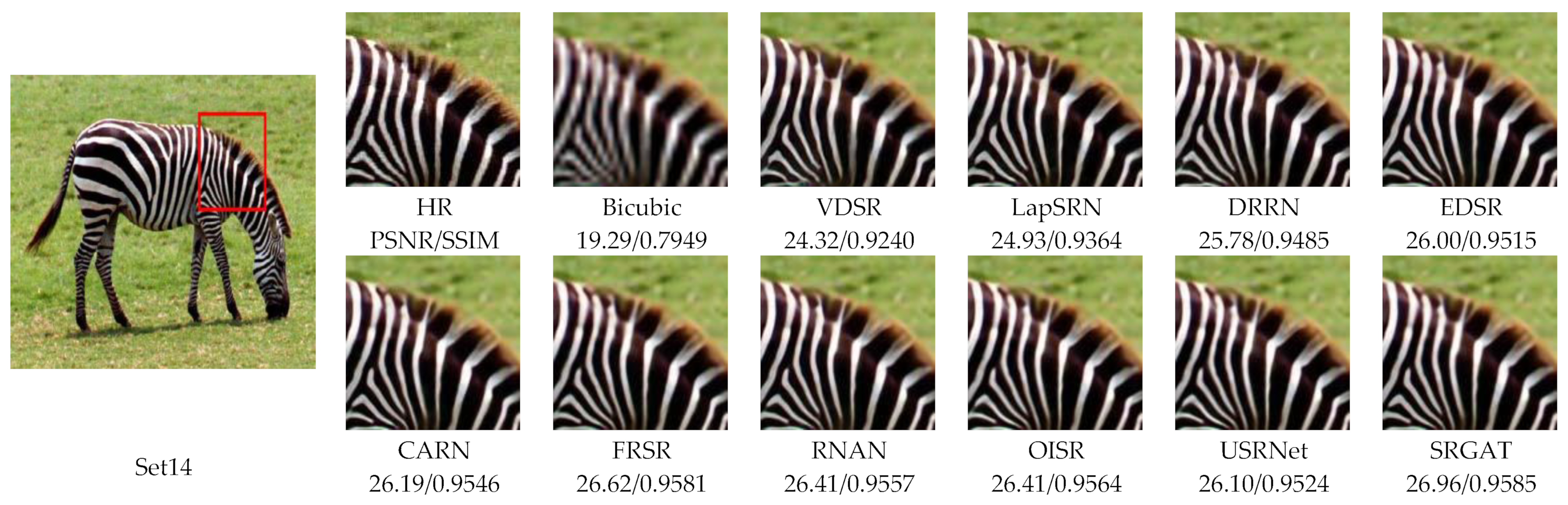
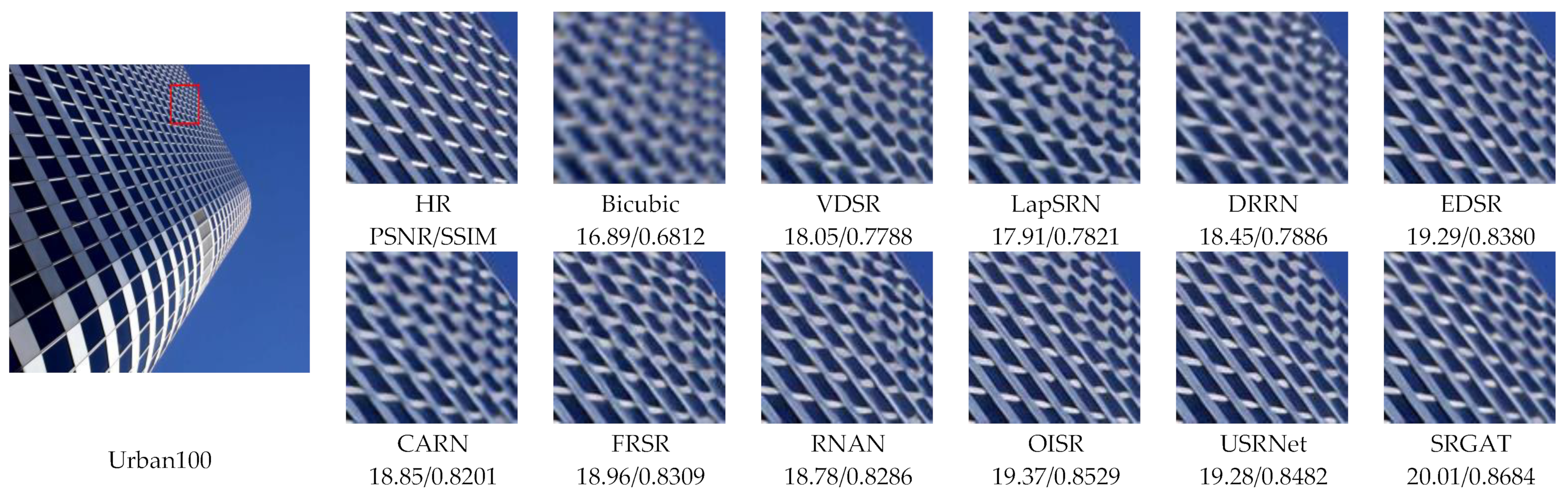
4.2.2. GCNs for Image Super-Resolution

To verify the super-resolution performance of some methods mentioned in Section 3.2, we conducted some experiments on the Set5, Set14, BSD100, Urban100, and Manga109 datasets in terms of quantitative and qualitative evaluations. We used PSNR and SSIM as evaluation metrics. The performance of various deep learning methods (such as SRCNN, VDSR, EDSR, RCAN, NLRN, SRFBN, SAN, RDN, USRNet, HAN, SRGAT, SCET, SwinIR, and RGCN) and traditional Bicubic interpolation (Bicubic) methods were compared on different benchmark test sets.
Table 19 shows the performance comparison of different methods under a magnification of two. Through data analysis, the following conclusions can be drawn: (1) Compared with the Bicubic method, the deep learning method has significant performance improvement in all test sets, showing higher PSNR and SSIM values. This means that the deep learning method can better restore the details and structural information of images when they require super-resolution reconstruction. (2) Among the tested deep learning models, RCAN, HAN, SwinIR, and other models have the best performance on most datasets, especially on Urban100 and Manga109 datasets. The PSNR and SSIM values of these models are relatively higher, reflecting their better recovery effect when dealing with complex scenes and rich textured images. Although the design principles and structures of various deep learning models are different, such as SRCNN, VCSR, ECSR, and RCAN focusing on residual learning; NLRN using non-local self-similarity; SRFBN using feedback mechanism; SAN, RDN, and HAN focusing on multi-level feature fusion; SRGAT introducing graph attention mechanism; SCET considering joint optimization in spatial and frequency domains; SwinIR using Transformer structure; and RGCN using graph convolutional network, these deep learning methods are generally better than traditional methods. In addition, with the evolution of technology, the performance of newly proposed models continues to be optimized and improved.
Table 20 shows the performance comparison of different methods under a magnification of three. The SwinlR method achieves the best results on multiple datasets, especially on Urban100 and Manga109 datasets, with PSNR and SSIM values far higher than other methods, indicating that SwinlR has excellent performance in super-resolution reconstruction of complex scenes and rich texture images. RCAN, HAN, RGCN, and other methods also perform well on most datasets. These advanced deep learning models effectively enhance the extraction and reconstruction ability of image features through residual connection, attention mechanism, graph convolution neural network, and other methods. Of course, compared with the traditional Bicubic method, all deep learning methods still achieve significant image super-resolution reconstruction performance under the three-fold magnification.
Table 21 shows the performance comparison of different methods when the magnification speed is four. Figure 13 and Figure 14. show the visual comparison of the Set14 dataset Urban100 dataset at a fourfold scale, respectively. Similarly, the SwinlR method achieves the best results on multiple datasets, especially on Urban100 and Manga109 datasets, where its PSNR and SSIM values are much higher than other methods. RCAN, HAN, RGCN, SRGAT, and other methods also perform well on most datasets. These advanced deep learning models effectively enhance the ability to extract and reconstruct image features through residual connection, attention mechanism, graph convolution neural network, and other methods.

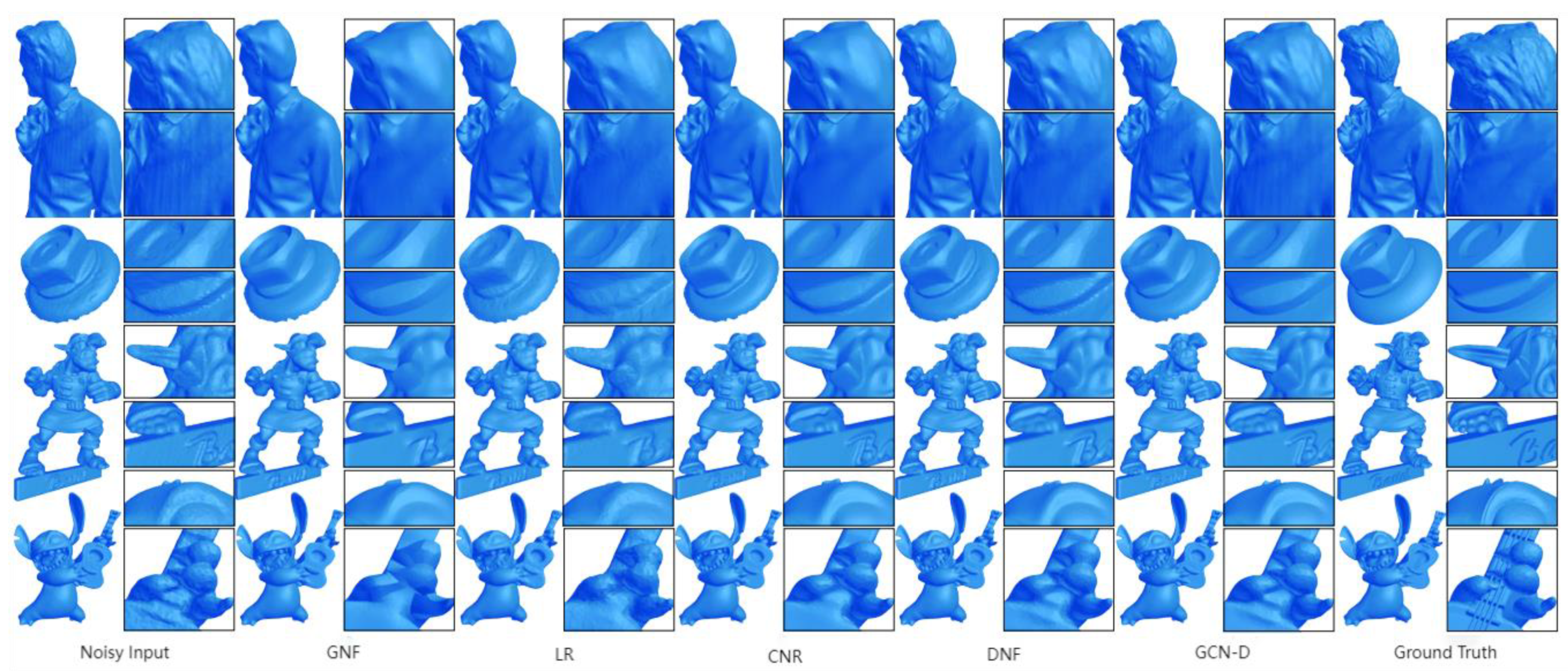
4.2.3. GCNs for Image Deblurring

To verify the deblurring performance of some methods mentioned in Section 3.3, we conducted some experiments on the Set5, Set14, BSD100, and Urban100 datasets in terms of quantitative and qualitative evaluations. We used PSNR and SSIM as evaluation metrics. The performance of various deep learning methods (such as SRCNN, FSRCNN, VDSR, RDN, D-DBPN, EDSR, and GCEDSR) were compared on different benchmark test sets. The detailed data are presented in Table 22.
As the magnification increases, the performance of all algorithms shows a downward trend, because more high-frequency details need to be recovered in the image magnification process, and the difficulty increases accordingly. The GCEDSR and EDSR methods have better deblurring performance under different magnification conditions.

5. Potential Research Points and Challenges

The application of GCNs in the field of image restoration is increasingly prevalent. This paper offers a concise introduction to these techniques to aid readers in understanding the methodologies involved. In this section, we delve further into the potential domains where GCNs can be harnessed for image restoration and highlight several unresolved issues within this context.

5.1. Potential Research Points

Image restoration techniques based on GCNs primarily aim to effectively enhance the performance and efficiency of image restoration processes and tackle complex image restoration tasks. Solutions for improving image restoration performance encompass:
  • Network Optimization: To enhance both the efficiency and effectiveness of image restoration, the structure of GCNs can be optimized. This encompasses designing deeper or wider network architectures, refining the construction method of graphs (e.g., considering more intricate relationships between pixels), adopting new activation functions, and regularization techniques to bolster learning capacity and generalization. Additionally, incorporating attention mechanisms enables GCNs to focus more keenly on critical regions in images, thereby improving restoration quality.
  • Multimodal Fusion: In image restoration tasks, supplementary information can often be obtained from various modalities (such as infrared images, depth images, etc.). GCNs can integrate these disparate modalities by constructing a unified graph representation, allowing the network to consider features from all modalities simultaneously. This approach can significantly improve recovery accuracy in specific scenarios, especially in complex scenes that traditional methods struggle with.
  • Applications in Complex Scenarios: GCNs are particularly adept at handling non-homogeneous and structured data in images, such as complex backgrounds or occlusions. Under such complex scenarios, adaptive graph structures can be constructed to better capture and leverage both local and global image information. For instance, in urban surveillance video restoration, GCNs can assist in recovering finer details in occluded regions by inferring obscured content based on learned environmental structural features.
  • Lightweight Network Design: To make GCNs suitable for resource-constrained devices like smartphones or embedded systems, lightweight design is necessary. This involves using fewer parameters, devising more efficient graph processing algorithms, or employing knowledge distillation techniques to simplify large-scale GCN models into smaller ones. A lightweight GCN not only reduces computational and storage demands but also accelerates the image restoration process, rendering it more practical.
  • Enhanced Feature Extraction Capabilities: While GCNs naturally excel at handling graph-structured data, effective feature extraction remains crucial in image restoration tasks. Integrating GCNs with other powerful feature extraction networks (like CNNs) could be considered to exploit GCNs’ ability to handle complex graph structures alongside CNNs’ efficiency in processing image data. Such a fusion can lead to further enhancements in the precision and robustness of image restoration.
  • Unsupervised or Semi-Supervised Learning: In many image restoration tasks, high-quality labeled data can be challenging to obtain. The development of GCNs can explore more unsupervised or semi-supervised learning strategies that leverage unlabeled or partially labeled data, reducing dependence on copious amounts of labeled data. For example, contrastive learning or self-supervised learning methods can enable models to learn effective image restoration strategies even without explicit supervision signals.
  • Cross-domain Image Restoration: GCNs can be employed in cross-domain image restoration tasks, such as restoring from one type of damage pattern (e.g., water damage) to another (e.g., cracks). Through cross-domain learning and transfer learning, GCNs can learn knowledge from one domain and apply it to another, which can dramatically boost model generalizability and practicality.
  • Integration of GCNs with Large Vision Models: The integration of GCNs with large vision models presents an exciting avenue for future research and development in the field of image restoration, including super-resolution. This synergy can leverage the strengths of both GCNs and large vision models to address the complexities of high-dimensional image data more effectively.
Combining GCNs with large vision models offers significant advantages. Large vision models, such as Vision Transformers (ViTs) [139], excel at extracting rich, hierarchical features, while GCNs are adept at capturing both global and local dependencies in graph-structured data. The integration of these approaches enhances performance in image super-resolution tasks, enables multi-scale and multi-modal learning, and improves feature aggregation efficiency through graph-based attention mechanisms. Currently, research is advancing in hybrid model architectures, transfer learning, and domain adaptation techniques to optimize the synergy between GCNs and large vision models [140]. However, future challenges include designing novel graph structures to better represent image data, improving model scalability and efficiency, and establishing comprehensive benchmarks and evaluation protocols to measure model performance. Overall, the combination of GCNs and large vision models holds promise for significant breakthroughs in image restoration but must overcome complexities and generalization issues in practical applications.

5.2. Challenges

Despite the promising potential of GCNs in the field of image restoration, they face several challenges during the application process:
  • Construction and Definition of Graph Structure: In GCNs, the structure of the graph is pivotal to model performance. In the context of image restoration, defining and constructing an effective graph structure poses a challenge since images are not inherently graph-structured data. Assigning pixels or image regions as nodes and determining their edges (connections) requires careful design to ensure that the graph structure accurately reflects the image content and degradation patterns.
  • Computational Costs for Large-Scale Image Processing: Images often have substantial sizes, implying that the graph constructed for image restoration might involve a vast number of nodes and edges. GCNs may encounter computational and storage efficiency issues when dealing with large-scale graph data. Optimizing algorithms and implementations, as well as employing hierarchical or multi-scale graph structures, are key to enhancing GCN’s performance in large-scale image processing.
  • Limitations in Feature Extraction: Although GCNs can effectively handle graph-structured data, they may have limitations in directly extracting useful features from raw image data. Compared to traditional image processing techniques such as convolutional neural networks, GCNs might be less powerful in processing pixel-level details and capturing complex texture patterns. Therefore, how to enhance GCN’s feature extraction capabilities or combine it with other techniques is a significant research direction.
  • Generalization Ability and Adaptability: The generalization capability of GCN models is particularly crucial for image restoration, as the types and degrees of image degradation in practical applications can vary widely. GCN models need to adapt to different damage conditions and image types, presenting challenges in terms of model design and diversity of training data.
  • Acquisition and Annotation Issues of Training Data: A substantial number of high-quality annotated data form the foundation for training effective GCN models. In the field of image restoration, obtaining ample pairs of degraded and undamaged images for training purposes can be difficult, especially for certain types of image degradation (e.g., historical document damages). Hence, how to leverage limited data or utilize unsupervised and semi-supervised learning methods to improve training effectiveness is another critical challenge for the development of GCNs.
These challenges outline the directions for the advancement of GCNs in the area of image restoration and pinpoint the issues researchers can explore and address in the future.

6. Conclusions

In this paper, we comprehensively compared, investigated, and summarized GCN techniques employed for image restoration. We began by presenting the fundamental framework of GCN technology applied to image restoration tasks. Subsequently, we provided an overview of the principal varieties of GCN methods currently utilized, analyzing their motivations and theoretical underpinnings, including but not limited to GraphSAGE and GATs. Then, we categorized and systematically summarized existing GCN technologies from three primary aspects: image denoising, image super-resolution, and image deblurring. Following this, we engaged in a comparative analysis, evaluating the performance, efficiency, and visual quality outcomes of different networks on benchmark datasets for image restoration purposes. Furthermore, we conducted cross-comparisons among diverse types of image restoration techniques. Lastly, we identified potential areas ripe for further investigation and discussed the challenges that GCN technology encounters within the context of image restoration, outlining avenues for future advancements in this domain.
The introduction of GCNs into image restoration has opened up new directions and presented novel challenges. Specifically, GCNs are adept at effectively handling pixel relationships and regional connectivity within images, which proves highly beneficial for restoring structural details and textural features in images. In the real world, the images being processed can be highly complex, requiring the simultaneous handling of noise reduction, deblurring, and other such issues. Moreover, there is a pressing need for models to be lightened, enhancing their generalization abilities and adaptability so that they are better suited for operation on mobile devices and edge devices. These are pressing challenges that researchers and scholars must address.

Author Contributions

Conceptualization, C.T.; Investigation, T.C.; Data curation, T.C.; Writing—original draft, T.C.; Writing—review & editing, T.B. and W.J. All authors have read and agreed to the published version of the manuscript.

Funding

This work was supported in part by Leading Talents in Gusu Innovation and Entrepreneurship Grant ZXL2023170, in part by projects supported by TCL science and technology innovation fund under Grant D5140240118.

Data Availability Statement

The authors confirm that the data supporting the findings of this study are available within the article.

Conflicts of Interest

The authors declare no conflict of interest.

References

  1. Jiao, Z.; Peng, X.; Wang, Y.; Xiao, J.; Nie, D.; Wu, X.; Wang, X.; Zhou, J.; Shen, D. TransDose: Transformer-based radiotherapy dose prediction from CT images guided by super-pixel-level GCN classification. Med. Image Anal. 2023, 89, 102902. [Google Scholar] [CrossRef] [PubMed]
  2. Chen, K.; Sun, J.; Shen, J.; Luo, J.; Zhang, X.; Pan, X.; Wu, D.; Zhao, Y.; Bento, M.; Ren, Y. GCN-MIF: Graph Convolutional Network with Multi-Information Fusion for Low-dose CT Denoising. arXiv 2021, arXiv:2105.07146. [Google Scholar]
  3. Liang, J.; Deng, Y.; Zeng, D. A deep neural network combined CNN and GCN for remote sensing scene classification. IEEE J. Sel. Top. Appl. Earth Obs. Remote Sens. 2020, 13, 4325–4338. [Google Scholar] [CrossRef]
  4. Chaudhuri, U.; Banerjee, B.; Bhattacharya, A.; Datcu, M. Attention-driven graph convolution network for remote sensing image retrieval. IEEE Geosci. Remote Sens. Lett. 2021, 19, 8019705. [Google Scholar] [CrossRef]
  5. Ma, C.; Zeng, S.; Li, D. Image restoration and enhancement in monitoring systems. In Proceedings of the 2020 International Conference on Intelligent Transportation, Big Data & Smart City (ICITBS), Vientiane, Laos, 11–12 January 2020; pp. 753–760. [Google Scholar]
  6. Ravikumar, S.; Bradley, A.; Thibos, L. Phase changes induced by optical aberrations degrade letter and face acuity. J. Vis. 2010, 10, 18. [Google Scholar] [CrossRef] [PubMed]
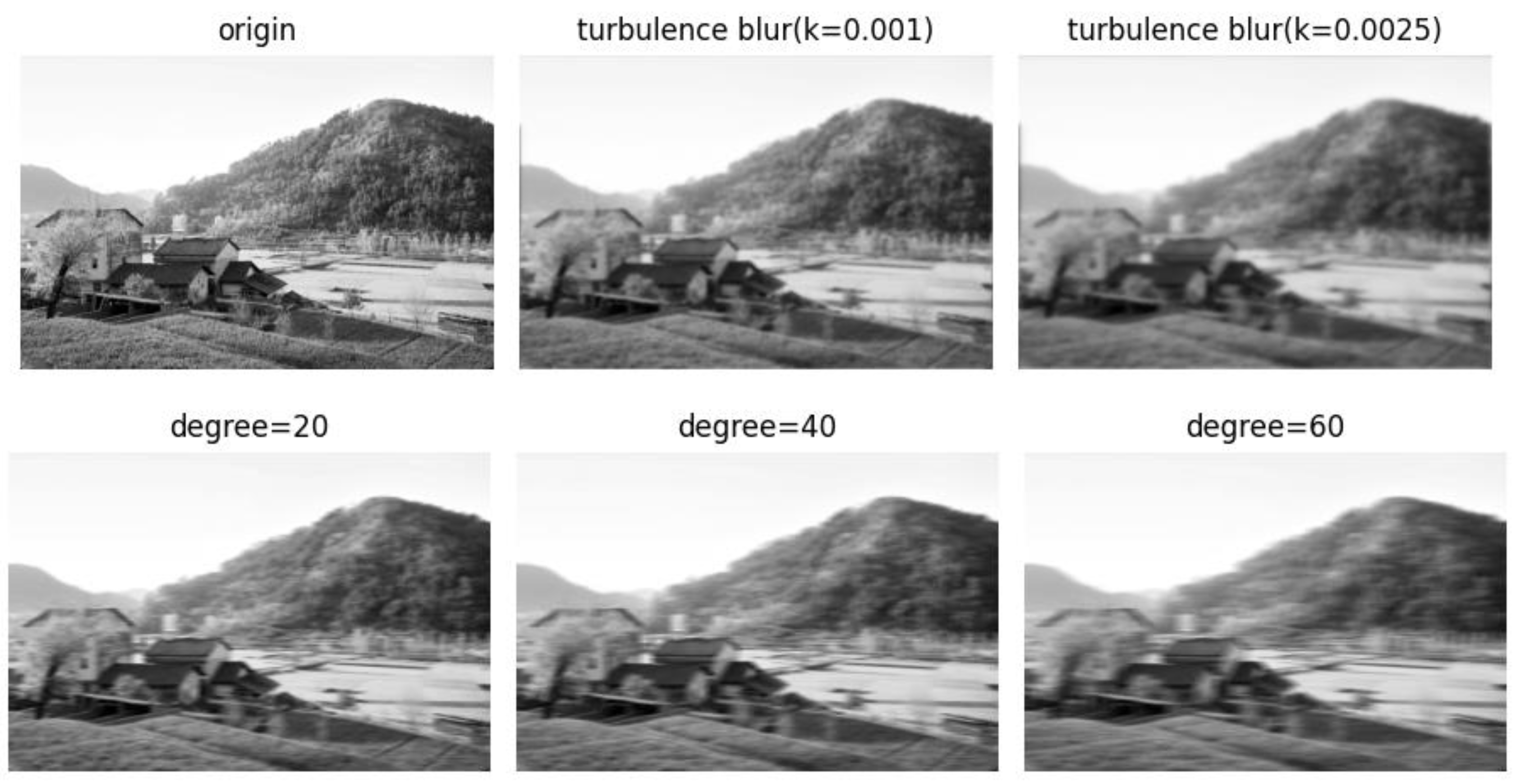
  7. Al-Hamadani, A.H.; Zainulabdeen, F.S.; Karam, G.S.; Nasir, E.Y.; Al-Saedi, A. Effects of atmospheric turbulence on the imaging performance of optical system. In Proceedings of the AIP Conference Proceedings, Beirut, Lebanon, 1–3 February 2018. [Google Scholar]
  8. Yang, X.; Li, S.; Cai, B.; Meng, Z.; Yan, J. MF-GCN: Motion Flow-Based Graph Network Learning Dynamics for Aerial IR Target Recognition. IEEE Trans. Aerosp. Electron. Syst. 2023, 59, 6346–6359. [Google Scholar] [CrossRef]
  9. Feng, R.; Li, C.; Chen, H.; Li, S.; Loy, C.C.; Gu, J. Removing diffraction image artifacts in under-display camera via dynamic skip connection network. In Proceedings of the IEEE/CVF Conference on Computer Vision and Pattern Recognition, Nashville, TN, USA, 20–25 June 2021; pp. 662–671. [Google Scholar]
  10. Diwakar, M.; Kumar, M. A review on CT image noise and its denoising. Biomed. Signal Process. Control 2018, 42, 73–88. [Google Scholar] [CrossRef]
  11. Wali, A.; Naseer, A.; Tamoor, M.; Gilani, S. Recent Progress in Digital Image Restoration Techniques: A Review. Digit. Signal Process. 2023, 141, 104187. [Google Scholar] [CrossRef]
  12. Zhou, Y.-T.; Chellappa, R.; Vaid, A.; Jenkins, B.K. Image restoration using a neural network. IEEE Trans. Acoust. Speech Signal Process. 1988, 36, 1141–1151. [Google Scholar] [CrossRef]
  13. Chang, J.-Y.; Chen, J.-L. Classifier-augmented median filters for image restoration. IEEE Trans. Instrum. Meas. 2004, 53, 351–356. [Google Scholar] [CrossRef]
  14. Baselice, F.; Ferraioli, G.; Ambrosanio, M.; Pascazio, V.; Schirinzi, G. Enhanced Wiener filter for ultrasound image restoration. Comput. Methods Programs Biomed. 2018, 153, 71–81. [Google Scholar] [CrossRef] [PubMed]
  15. Khan, M.M.R.; Sakib, S.; Arif, R.B.; Siddique, M.A.B. Digital image restoration in matlab: A case study on inverse and wiener filtering. In Proceedings of the 2018 International Conference on Innovation in Engineering and Technology (ICIET), Osaka, Japan, 6–8 January 2018; pp. 1–6. [Google Scholar]
  16. Zhang, B.; Wang, M.; Pan, J. Image restoration based on Kalman filter. In Proceedings of the 2013 IEEE International Geoscience and Remote Sensing Symposium-IGARSS, Melbourne, Australia, 21–26 July 2013; pp. 497–500. [Google Scholar]
  17. Chen, L.-Y.; Wang, C.; Xiao, X.-Y.; Ren, C.; Zhang, D.-J.; Li, Z.; Cao, D.-Z. Denoising in SVD-based ghost imaging. Opt. Express 2022, 30, 6248–6257. [Google Scholar] [CrossRef] [PubMed]
  18. Bian, Z.; Ma, J.; Huang, J.; Zhang, H.; Niu, S.; Feng, Q.; Liang, Z.; Chen, W. SR-NLM: A sinogram restoration induced non-local means image filtering for low-dose computed tomography. Comput. Med. Imaging Graph. 2013, 37, 293–303. [Google Scholar] [CrossRef] [PubMed]
  19. Eksioglu, E.M. Decoupled algorithm for MRI reconstruction using nonlocal block matching model: BM3D-MRI. J. Math. Imaging Vis. 2016, 56, 430–440. [Google Scholar] [CrossRef]
  20. Zha, Z.; Yuan, X.; Zhou, J.; Zhu, C.; Wen, B. Image restoration via simultaneous nonlocal self-similarity priors. IEEE Trans. Image Process. 2020, 29, 8561–8576. [Google Scholar] [CrossRef] [PubMed]
  21. Mairal, J.; Bach, F.; Ponce, J.; Sapiro, G.; Zisserman, A. Non-local sparse models for image restoration. In Proceedings of the 2009 IEEE 12th International Conference on Computer Vision, Kyoto, Japan, 27 September–4 October 2009; pp. 2272–2279. [Google Scholar]
  22. Cho, T.S.; Zitnick, C.L.; Joshi, N.; Kang, S.B.; Szeliski, R.; Freeman, W.T. Image restoration by matching gradient distributions. IEEE Trans. Pattern Anal. Mach. Intell. 2011, 34, 683–694. [Google Scholar]
  23. Pleschberger, M.; Schrunner, S.; Pilz, J. An explicit solution for image restoration using Markov random fields. J. Signal Process. Syst. 2020, 92, 257–267. [Google Scholar] [CrossRef]
  24. Zhang, K.; Zuo, W.; Gu, S.; Zhang, L. Learning deep CNN denoiser prior for image restoration. In Proceedings of the IEEE Conference on Computer Vision and Pattern Recognition, Honolulu, HI, USA, 21–26 July 2017; pp. 3929–3938. [Google Scholar]
  25. Zhang, K.; Gao, X.; Tao, D.; Li, X. Single image super-resolution with non-local means and steering kernel regression. IEEE Trans. Image Process. 2012, 21, 4544–4556. [Google Scholar] [CrossRef] [PubMed]
  26. Liu, D.; Wen, B.; Fan, Y.; Loy, C.C.; Huang, T.S. Non-local recurrent network for image restoration. arXiv 2018, arXiv:1806.02919. [Google Scholar]
  27. Zhang, K.; Zuo, W.; Chen, Y.; Meng, D.; Zhang, L. Beyond a gaussian denoiser: Residual learning of deep cnn for image denoising. IEEE Trans. Image Process. 2017, 26, 3142–3155. [Google Scholar] [CrossRef]
  28. Zhang, K.; Zuo, W.; Zhang, L. FFDNet: Toward a fast and flexible solution for CNN-based image denoising. IEEE Trans. Image Process. 2018, 27, 4608–4622. [Google Scholar] [CrossRef] [PubMed]
  29. Guo, S.; Yan, Z.; Zhang, K.; Zuo, W.; Zhang, L. Toward convolutional blind denoising of real photographs. In Proceedings of the IEEE/CVF Conference on Computer Vision and Pattern Recognition, Long Beach, CA, USA, 15–20 June 2019; pp. 1712–1722. [Google Scholar]
  30. Zhang, K.; Zuo, W.; Zhang, L. Learning a single convolutional super-resolution network for multiple degradations. In Proceedings of the IEEE Conference on Computer Vision and Pattern Recognition, Salt Lake City, UT, USA, 18–23 June 2018; pp. 3262–3271. [Google Scholar]
  31. Asif, N.A.; Sarker, Y.; Chakrabortty, R.K.; Ryan, M.J.; Ahamed, M.H.; Saha, D.K.; Badal, F.R.; Das, S.K.; Ali, M.F.; Moyeen, S.I. Graph neural network: A comprehensive review on non-euclidean space. IEEE Access 2021, 9, 60588–60606. [Google Scholar] [CrossRef]
  32. Battaglia, P.W.; Hamrick, J.B.; Bapst, V.; Sanchez-Gonzalez, A.; Zambaldi, V.; Malinowski, M.; Tacchetti, A.; Raposo, D.; Santoro, A.; Faulkner, R. Relational inductive biases, deep learning, and graph networks. arXiv 2018, arXiv:1806.01261. [Google Scholar]
  33. Bruna, J.; Zaremba, W.; Szlam, A.; LeCun, Y. Spectral networks and locally connected networks on graphs. arXiv 2013, arXiv:1312.6203. [Google Scholar]
  34. Liu, J.; Gong, M.; Miao, Q.; Wang, X.; Li, H. Structure learning for deep neural networks based on multiobjective optimization. IEEE Trans. Neural Netw. Learn. Syst. 2017, 29, 2450–2463. [Google Scholar] [CrossRef]
  35. Coşkun, M.; Uçar, A.; Yildirim, Ö.; Demir, Y. Face recognition based on convolutional neural network. In Proceedings of the 2017 International Conference on Modern Electrical and Energy Systems (MEES), Kremenchuk, Ukraine, 15–17 November 2017; pp. 376–379. [Google Scholar]
  36. Zhang, S.; Tong, H.; Xu, J.; Maciejewski, R. Graph convolutional networks: A comprehensive review. Comput. Soc. Netw. 2019, 6, 11. [Google Scholar] [CrossRef]
  37. Defferrard, M.; Bresson, X.; Vandergheynst, P. Convolutional neural networks on graphs with fast localized spectral filtering. Adv. Neural Inf. Process. Syst. 2016, 29, 3844–3852. [Google Scholar]
  38. Kipf, T.N.; Welling, M. Semi-supervised classification with graph convolutional networks. arXiv 2016, arXiv:1609.02907. [Google Scholar]
  39. Yu, J.; Yin, H.; Li, J.; Gao, M.; Huang, Z.; Cui, L. Enhancing social recommendation with adversarial graph convolutional networks. IEEE Trans. Knowl. Data Eng. 2020, 34, 3727–3739. [Google Scholar] [CrossRef]
  40. Hamilton, W.; Ying, Z.; Leskovec, J. Inductive representation learning on large graphs. Adv. Neural Inf. Process. Syst. 2017, 30, 1024–1034. [Google Scholar]
  41. Velickovic, P.; Cucurull, G.; Casanova, A.; Romero, A.; Lio, P.; Bengio, Y. Graph attention networks. Stat 2017, 1050, 10-48550. [Google Scholar]
  42. Jiang, B.; Lu, Y.; Chen, X.; Lu, X.; Lu, G. Graph attention in attention network for image denoising. IEEE Trans. Syst. Man Cybern. Syst. 2023, 53, 7077–7088. [Google Scholar] [CrossRef]
  43. Zhang, J.; Zhang, M.; Lu, Z.; Xiang, T. Adargcn: Adaptive aggregation gcn for few-shot learning. In Proceedings of the IEEE/CVF Winter Conference on Applications of Computer Vision, Virtual, 5–9 January 2021; pp. 3482–3491. [Google Scholar]
  44. Li, Y.; Fu, X.; Zha, Z.-J. Cross-patch graph convolutional network for image denoising. In Proceedings of the IEEE/CVF International Conference on Computer Vision, Montreal, QC, Canada, 11–17 October 2021; pp. 4651–4660. [Google Scholar]
  45. Han, W. Robust Graph Embedding via Self-Supervised Graph Denoising. In Proceedings of the 2022 19th International Computer Conference on Wavelet Active Media Technology and Information Processing (ICCWAMTIP), Chengdu, China, 16–18 December 2022; pp. 1–4. [Google Scholar]
  46. Mou, C.; Zhang, J. Graph attention neural network for image restoration. In Proceedings of the 2021 IEEE International Conference on Multimedia and Expo (ICME), Shenzhen, China, 5–9 July 2021; pp. 1–6. [Google Scholar]
  47. Mou, C.; Zhang, J.; Wu, Z. Dynamic attentive graph learning for image restoration. In Proceedings of the IEEE/CVF International Conference on Computer Vision, Montreal, Canada, 11–17 October 2021; pp. 4328–4337. [Google Scholar]
  48. Liu, H.; Liao, P.; Chen, H.; Zhang, Y. ERA-WGAT: Edge-enhanced residual autoencoder with a window-based graph attention convolutional network for low-dose CT denoising. Biomed. Opt. Express 2022, 13, 5775–5793. [Google Scholar] [CrossRef] [PubMed]
  49. Shen, Y.; Fu, H.; Du, Z.; Chen, X.; Burnaev, E.; Zorin, D.; Zhou, K.; Zheng, Y. GCN-denoiser: Mesh denoising with graph convolutional networks. ACM Trans. Graph. (TOG) 2022, 41, 1–14. [Google Scholar] [CrossRef]
  50. Armando, M.; Franco, J.-S.; Boyer, E. Mesh denoising with facet graph convolutions. IEEE Trans. Vis. Comput. Graph. 2020, 28, 2999–3012. [Google Scholar] [CrossRef] [PubMed]
  51. Mostafa, H.; Nassar, M. Permutohedral-gcn: Graph convolutional networks with global attention. arXiv 2020, arXiv:2003.00635. [Google Scholar]
  52. Tian, C.; Zheng, M.; Li, B.; Zhang, Y.; Zhang, S.; Zhang, D. Perceptive self-supervised learning network for noisy image watermark removal. IEEE Trans. Circuits Syst. Video Technol. 2024. [Google Scholar] [CrossRef]
  53. Zhao, Z.; Wu, W.; Liu, H.; Gong, Y. A Multi-Stream Network for Mesh Denoising Via Graph Neural Networks with Gaussian Curvature. In Proceedings of the 2023 IEEE International Conference on Image Processing (ICIP), Kuala Lumpur, Malaysia, 8–11 October 2023; pp. 1355–1359. [Google Scholar]
  54. Chen, Y.-J.; Tsai, C.-Y.; Xu, X.; Shi, Y.; Ho, T.-Y.; Huang, M.; Yuan, H.; Zhuang, J. Ct image denoising with encoder-decoder based graph convolutional networks. In Proceedings of the 2021 IEEE 18th International Symposium on Biomedical Imaging (ISBI), Nice, France, 13–16 April 2021; pp. 400–404. [Google Scholar]
  55. Chen, Z.; Li, P.; Wei, Z.; Chen, H.; Xie, H.; Wei, M.; Wang, F.L. Geogcn: Geometric Dual-Domain Graph Convolution Network For Point Cloud Denoising. In Proceedings of the ICASSP 2023—2023 IEEE International Conference on Acoustics, Speech and Signal Processing (ICASSP), Rhodes Island, Greece, 4–10 June 2023; pp. 1–5. [Google Scholar]
  56. Fu, X.; Qi, Q.; Zha, Z.-J.; Ding, X.; Wu, F.; Paisley, J. Successive graph convolutional network for image de-raining. Int. J. Comput. Vis. 2021, 129, 1691–1711. [Google Scholar] [CrossRef]
  57. Chen, K.; Pu, X.; Ren, Y.; Qiu, H.; Li, H.; Sun, J. Low-dose ct image blind denoising with graph convolutional networks. In Proceedings of the International Conference on Neural Information Processing, Bangkok, Thailand, 18–22 November 2020; pp. 423–435. [Google Scholar]
  58. Liu, Q.; Xiao, L.; Yang, J.; Wei, Z. CNN-enhanced graph convolutional network with pixel-and superpixel-level feature fusion for hyperspectral image classification. IEEE Trans. Geosci. Remote Sens. 2020, 59, 8657–8671. [Google Scholar] [CrossRef]
  59. Tian, C.; Zheng, M.; Zuo, W.; Zhang, S.; Zhang, Y.; Lin, C.-W. A cross Transformer for image denoising. Inf. Fusion 2024, 102, 102043. [Google Scholar] [CrossRef]
  60. Jiang, B.; Lu, Y.; Zhang, B.; Lu, G. AGP-Net: Adaptive Graph Prior Network for Image Denoising. IEEE Trans. Ind. Inform. 2023, 20, 4753–4764. [Google Scholar] [CrossRef]
  61. Eliasof, M.; Haber, E.; Treister, E. Pde-gcn: Novel architectures for graph neural networks motivated by partial differential equations. Adv. Neural Inf. Process. Syst. 2021, 34, 3836–3849. [Google Scholar]
  62. Hattori, S.; Yatagawa, T.; Ohtake, Y.; Suzuki, H. Learning self-prior for mesh denoising using dual graph convolutional networks. In Proceedings of the European Conference on Computer Vision, Tel Aviv, Israel, 23–27 October 2022; pp. 363–379. [Google Scholar]
  63. Fu, X.; Qi, Q.; Zha, Z.-J.; Zhu, Y.; Ding, X. Rain streak removal via dual graph convolutional network. In Proceedings of the AAAI Conference on Artificial Intelligence, Virtually, 2–9 February 2021; pp. 1352–1360. [Google Scholar]
  64. Yang, Y.; Qi, Y. Image super-resolution via channel attention and spatial graph convolutional network. Pattern Recognit. 2021, 112, 107798. [Google Scholar] [CrossRef]
  65. Yan, Y.; Ren, W.; Hu, X.; Li, K.; Shen, H.; Cao, X. SRGAT: Single image super-resolution with graph attention network. IEEE Trans. Image Process. 2021, 30, 4905–4918. [Google Scholar] [CrossRef] [PubMed]
  66. Yang, Y.; Qi, Y. Spatial Graph Convolutional Network for Image Super-Resolution. In Proceedings of the 2021 IEEE International Conference on Multimedia and Expo (ICME), Shenzhen, China, 5–9 July 2021; pp. 1–6. [Google Scholar]
  67. Zhang, Y.; Li, K.; Li, K.; Fu, Y. MR image super-resolution with squeeze and excitation reasoning attention network. In Proceedings of the IEEE/CVF Conference on Computer Vision and Pattern Recognition, Nashville, TN, USA, 19–25 June 2021; pp. 13425–13434. [Google Scholar]
  68. Wu, H.; Zhang, J.; Huang, K. Point cloud super resolution with adversarial residual graph networks. arXiv 2019, arXiv:1908.02111. [Google Scholar]
  69. Chen, T.; Qiu, Z.; Zhang, C.; Bai, H. Graph Convolution Point Cloud Super-Resolution Network Based on Mixed Attention Mechanism. Electronics 2023, 12, 2196. [Google Scholar] [CrossRef]
  70. Liang, G.; KinTak, U.; Yin, H.; Liu, J.; Luo, H. Multi-scale hybrid attention graph convolution neural network for remote sensing images super-resolution. Signal Process. 2023, 207, 108954. [Google Scholar] [CrossRef]
  71. Qian, G.; Abualshour, A.; Li, G.; Thabet, A.; Ghanem, B. Pu-gcn: Point cloud upsampling using graph convolutional networks. In Proceedings of the IEEE/CVF Conference on Computer Vision and Pattern Recognition, Virtual, 19–25 June 2021; pp. 11683–11692. [Google Scholar]
  72. Zhong, F.; Bai, Z. PSR-GAT: Arbitrary point cloud super-resolution using graph attention networks. Multimed. Tools Appl. 2024, 83, 26213–26232. [Google Scholar] [CrossRef]
  73. Cao, Q.; Tang, P.; Wang, H. Spatio-temporal Super-resolution Network: Enhance Visual Representations for Video Captioning. In Proceedings of the 2022 IEEE International Symposium on Circuits and Systems (ISCAS), Austin, TX, USA, 27 May–1 June 2022; pp. 3125–3129. [Google Scholar]
  74. Berlincioni, L.; Berretti, S.; Bertini, M.; Bimbo, A.D. 4DSR-GCN: 4D Video Point Cloud Upsampling using Graph Convolutional Networks. In Proceedings of the 1st International Workshop on Multimedia Content Generation and Evaluation: New Methods and Practice, Ottawa, ON, Canada, 29 October 2023; pp. 57–65. [Google Scholar]
  75. Yang, Y.; Qi, Y.; Qi, S. Relation-consistency graph convolutional network for image super-resolution. Vis. Comput. 2024, 40, 619–635. [Google Scholar] [CrossRef]
  76. Zhang, Y.; Wei, D.; Qin, C.; Wang, H.; Pfister, H.; Fu, Y. Context reasoning attention network for image super-resolution. In Proceedings of the IEEE/CVF International Conference on Computer Vision, Montreal, BC, Canada, 11–17 October 2021; pp. 4278–4287. [Google Scholar]
  77. Tian, C.; Zhang, X.; Zhang, Q.; Yang, M.; Ju, Z. Image super-resolution via dynamic network. CAAI Trans. Intell. Technol. 2023. [Google Scholar] [CrossRef]
  78. Liu, B.; Zhao, L.; Shao, S.; Liu, W.; Tao, D.; Cao, W.; Zhou, Y. RAN: Region-Aware Network for Remote Sensing Image Super-Resolution. IEEE Trans. Geosci. Remote Sens. 2023, 61, 5408113. [Google Scholar] [CrossRef]
  79. You, C.; Han, L.; Feng, A.; Zhao, R.; Tang, H.; Fan, W. Megan: Memory enhanced graph attention network for space-time video super-resolution. In Proceedings of the IEEE/CVF Winter Conference on Applications of Computer Vision, Waikoloa, HI, USA, 3–8 January 2022; pp. 1401–1411. [Google Scholar]
  80. Liu, Z.; Zhang, C.; Wu, Y.; Zhang, C. Joint face completion and super-resolution using multi-scale feature relation learning. J. Vis. Commun. Image Represent. 2023, 93, 103806. [Google Scholar] [CrossRef]
  81. Zhang, Y.; Wei, D.; Schalek, R.; Wu, Y.; Turney, S.; Lichtman, J.; Pfister, H.; Fu, Y. High-throughput microscopy image deblurring with graph reasoning attention network. In Proceedings of the 2023 IEEE 20th International Symposium on Biomedical Imaging (ISBI), Cartagena, Colombia, 18–21 April 2023; pp. 1–5. [Google Scholar]
  82. Xu, B.; Yin, H. Graph convolutional networks in feature space for image deblurring and super-resolution. In Proceedings of the 2021 International Joint Conference on Neural Networks (IJCNN), Virtual, 18–22 July 2021; pp. 1–8. [Google Scholar]
  83. Zhang, A.; Ren, W.; Liu, Y.; Cao, X. Lightweight Image Super-Resolution with Superpixel Token Interaction. In Proceedings of the IEEE/CVF International Conference on Computer Vision, Paris, France, 1–6 October 2023; pp. 12728–12737. [Google Scholar]
  84. Li, H.; Yang, Y.; Chang, M.; Chen, S.; Feng, H.; Xu, Z.; Li, Q.; Chen, Y. Srdiff: Single image super-resolution with diffusion probabilistic models. Neurocomputing 2022, 479, 47–59. [Google Scholar] [CrossRef]
  85. Liu, Z.; Li, L.; Wu, Y.; Zhang, C. Facial expression restoration based on improved graph convolutional networks. In Proceedings of the MultiMedia Modeling: 26th International Conference, MMM 2020, Daejeon, Republic of Korea, 5–8 January 2020; Proceedings, Part II 26, 2020. pp. 527–539. [Google Scholar]
  86. Yue, Z.; Shi, M. Enhancing Space-time Video Super-resolution via Spatial-temporal Feature Interaction. arXiv 2022, arXiv:2207.08960. [Google Scholar]
  87. Liao, L.; Zhang, Z.; Xia, S. RAID-Net: Region-Aware Image Deblurring Network Under Guidance of the Image Blur Formulation. IEEE Access 2022, 10, 83940–83948. [Google Scholar] [CrossRef]
  88. Chen, S.; Zhang, W.; Li, Z.; Wang, Y.; Zhang, B. Cloud Removal with SAR-Optical Data Fusion and Graph-Based Feature Aggregation Network. Remote Sens. 2022, 14, 3374. [Google Scholar] [CrossRef]
  89. Shen, H.; Jiang, M.; Li, J.; Zhou, C.; Yuan, Q.; Zhang, L. Coupling model-and data-driven methods for remote sensing image restoration and fusion: Improving physical interpretability. IEEE Geosci. Remote Sens. Mag. 2022, 10, 231–249. [Google Scholar] [CrossRef]
  90. Li, X.; Jin, X.; Fu, J.; Yu, X.; Tong, B.; Chen, Z. Few-Shot Real Image Super-resolution via Distortion-Relation Guided Transfer Learning. arXiv 2021, arXiv:2111.13078. [Google Scholar]
  91. Li, Y.; Wang, N.; Li, J.; Zhang, Y. WIG-Net: Wavelet-Based Defocus Deblurring with IFA and GCN. Appl. Sci. 2023, 13, 12513. [Google Scholar] [CrossRef]
  92. Yang, J.; Jin, H.; Tang, R.; Han, X.; Feng, Q.; Jiang, H.; Zhong, S.; Yin, B.; Hu, X. Harnessing the power of llms in practice: A survey on chatgpt and beyond. ACM Trans. Knowl. Discov. Data 2024, 18, 1–32. [Google Scholar] [CrossRef]
  93. Yin, Z.; Wang, J.; Cao, J.; Shi, Z.; Liu, D.; Li, M.; Huang, X.; Wang, Z.; Sheng, L.; Bai, L. Lamm: Language-assisted multi-modal instruction-tuning dataset, framework, and benchmark. arXiv 2024, arXiv:2306.06687. [Google Scholar]
  94. Chen, Z.; Mao, H.; Li, H.; Jin, W.; Wen, H.; Wei, X.; Wang, S.; Yin, D.; Fan, W.; Liu, H. Exploring the potential of large language models (llms) in learning on graphs. ACM SIGKDD Explor. Newsl. 2024, 25, 42–61. [Google Scholar] [CrossRef]
  95. Jin, X.; Shi, Y.; Xia, B.; Yang, W. LLMRA: Multi-modal Large Language Model based Restoration Assistant. arXiv 2024, arXiv:2401.11401. [Google Scholar]
  96. Wei, Y.; Zhang, Z.; Ren, J.; Xu, X.; Hong, R.; Yang, Y.; Yan, S.; Wang, M. Clarity ChatGPT: An Interactive and Adaptive Processing System for Image Restoration and Enhancement. arXiv 2023, arXiv:2311.11695. [Google Scholar]
  97. Fan, W.; Wang, S.; Huang, J.; Chen, Z.; Song, Y.; Tang, W.; Mao, H.; Liu, H.; Liu, X.; Yin, D. Graph Machine Learning in the Era of Large Language Models (LLMs). arXiv 2024, arXiv:2404.14928. [Google Scholar]
  98. Arbelaez, P.; Maire, M.; Fowlkes, C.; Malik, J. Contour detection and hierarchical image segmentation. IEEE Trans. Pattern Anal. Mach. Intell. 2010, 33, 898–916. [Google Scholar] [CrossRef]
  99. Valsesia, D.; Fracastoro, G.; Magli, E. Deep graph-convolutional image denoising. IEEE Trans. Image Process. 2020, 29, 8226–8237. [Google Scholar] [CrossRef] [PubMed]
  100. Huang, J.-B.; Singh, A.; Ahuja, N. Single image super-resolution from transformed self-exemplars. In Proceedings of the IEEE Conference on Computer Vision and Pattern Recognition, Boston, MA, USA, 7–12 June 2015; pp. 5197–5206. [Google Scholar]
  101. Dabov, K.; Foi, A.; Katkovnik, V.; Egiazarian, K. Image denoising by sparse 3-D transform-domain collaborative filtering. IEEE Trans. Image Process. 2007, 16, 2080–2095. [Google Scholar] [CrossRef] [PubMed]
  102. Abdelhamed, A.; Lin, S.; Brown, M.S. A high-quality denoising dataset for smartphone cameras. In Proceedings of the IEEE Conference on Computer Vision and Pattern Recognition, Salt Lake City, UT, USA, 18–23 June 2018; pp. 1692–1700. [Google Scholar]
  103. Agustsson, E.; Timofte, R. Ntire 2017 challenge on single image super-resolution: Dataset and study. In Proceedings of the IEEE Conference on Computer Vision and Pattern Recognition Workshops, Honolulu, HI, USA, 21–26 July 2017; pp. 126–135. [Google Scholar]
  104. Martin, D.; Fowlkes, C.; Tal, D.; Malik, J. A database of human segmented natural images and its application to evaluating segmentation algorithms and measuring ecological statistics. In Proceedings of the Proceedings Eighth IEEE International Conference on Computer Vision. ICCV 2001, Vancouver, BC, Canada, 7–14 July 2001; pp. 416–423. [Google Scholar]
  105. Yang, W.; Tan, R.T.; Feng, J.; Liu, J.; Guo, Z.; Yan, S. Deep joint rain detection and removal from a single image. In Proceedings of the IEEE Conference on Computer Vision and Pattern Recognition, Honolulu, HI, USA, 21–26 July 2017; pp. 1357–1366. [Google Scholar]
  106. Zhang, H.; Sindagi, V.; Patel, V.M. Image de-raining using a conditional generative adversarial network. IEEE Trans. Circuits Syst. Video Technol. 2019, 30, 3943–3956. [Google Scholar] [CrossRef]
  107. Bevilacqua, M.; Roumy, A.; Guillemot, C.; Alberi-Morel, M.L. Low-complexity single-image super-resolution based on nonnegative neighbor embedding. In Proceedings of the 23rd British Machine Vision Conference (BMVC), Surrey, UK, 3–7 September 2012. [Google Scholar]
  108. Zeyde, R.; Elad, M.; Protter, M. On single image scale-up using sparse-representations. In Proceedings of the Curves and Surfaces: 7th International Conference, Avignon, France, 24–30 June 2010; Revised Selected Papers 7, 2012. pp. 711–730. [Google Scholar]
  109. Matsui, Y.; Ito, K.; Aramaki, Y.; Fujimoto, A.; Ogawa, T.; Yamasaki, T.; Aizawa, K. Sketch-based manga retrieval using manga109 dataset. Multimed. Tools Appl. 2017, 76, 21811–21838. [Google Scholar] [CrossRef]
  110. Cruz-Neira, C.; Sandin, D.J.; DeFanti, T.A.; Kenyon, R.V.; Hart, J.C. The CAVE: Audio visual experience automatic virtual environment. Commun. ACM 1992, 35, 64–73. [Google Scholar] [CrossRef]
  111. Chua, T.-S.; Tang, J.; Hong, R.; Li, H.; Luo, Z.; Zheng, Y. Nus-wide: A real-world web image database from national university of singapore. In Proceedings of the ACM International Conference on Image and Video Retrieval, Santorini, Greece, 8–10 July 2009; pp. 1–9. [Google Scholar]
  112. Ancuti, C.; Ancuti, C.O.; Timofte, R. Ntire 2018 challenge on image dehazing: Methods and results. In Proceedings of the IEEE Conference on Computer Vision and Pattern Recognition Workshops, Salt Lake City, UT, USA, 18–23 June 2018; pp. 891–901. [Google Scholar]
  113. Visionair. Available online: https://vision-air.github.io/ (accessed on 14 November 2017).
  114. Cheng, S.; Liu, R.; He, Y.; Fan, X.; Luo, Z. Blind image deblurring via hybrid deep priors modeling. Neurocomputing 2020, 387, 334–345. [Google Scholar] [CrossRef]
  115. Lim, B.; Son, S.; Kim, H.; Nah, S.; Mu Lee, K. Enhanced deep residual networks for single image super-resolution. In Proceedings of the IEEE Conference on Computer Vision and Pattern Recognition Workshops, Honolulu, HI, USA, 21–26 July 2017; pp. 136–144. [Google Scholar]
  116. Yang, H.; Zhou, D.; Li, M.; Zhao, Q. A two-stage network with wavelet transformation for single-image deraining. Vis. Comput. 2023, 39, 3887–3903. [Google Scholar] [CrossRef]
  117. Chang, Y.; Yan, L.; Zhong, S. Transformed low-rank model for line pattern noise removal. In Proceedings of the IEEE International Conference on Computer Vision, Venice, Italy, 22–29 October 2017; pp. 1726–1734. [Google Scholar]
  118. Wang, T.; Yang, X.; Xu, K.; Chen, S.; Zhang, Q.; Lau, R.W. Spatial attentive single-image deraining with a high quality real rain dataset. In Proceedings of the IEEE/CVF Conference on Computer Vision and Pattern Recognition, Long Beach, CA, USA, 15–20 June 2019; pp. 12270–12279. [Google Scholar]
  119. Wang, P.-S.; Liu, Y.; Tong, X. Mesh denoising via cascaded normal regression. ACM Trans. Graph. 2016, 35, 1–12. [Google Scholar] [CrossRef]
  120. Wang, Y.; Sun, Y.; Liu, Z.; Sarma, S.E.; Bronstein, M.M.; Solomon, J.M. Dynamic graph cnn for learning on point clouds. ACM Trans. Graph. (Tog) 2019, 38, 1–12. [Google Scholar] [CrossRef]
  121. Liu, P.; Zhang, H.; Zhang, K.; Lin, L.; Zuo, W. Multi-level wavelet-CNN for image restoration. In Proceedings of the IEEE Conference on Computer Vision and Pattern Recognition Workshops, Salt Lake City, UT, USA, 18–22 June 2018; pp. 773–782. [Google Scholar]
  122. Devalla, S.K.; Renukanand, P.K.; Sreedhar, B.K.; Subramanian, G.; Zhang, L.; Perera, S.; Mari, J.-M.; Chin, K.S.; Tun, T.A.; Strouthidis, N.G. DRUNET: A dilated-residual U-Net deep learning network to segment optic nerve head tissues in optical coherence tomography images. Biomed. Opt. Express 2018, 9, 3244–3265. [Google Scholar] [CrossRef] [PubMed]
  123. Jiang, B.; Li, J.; Li, H.; Li, R.; Zhang, D.; Lu, G. Enhanced frequency fusion network with dynamic hash attention for image denoising. Inf. Fusion 2023, 92, 420–434. [Google Scholar] [CrossRef]
  124. Ward, C.M.; Harguess, J.; Crabb, B.; Parameswaran, S. Image quality assessment for determining efficacy and limitations of Super-Resolution Convolutional Neural Network (SRCNN). In Proceedings of the Applications of Digital Image Processing XL, San Diego, CA, USA, 7–10 August 2017; pp. 19–30. [Google Scholar]
  125. Kim, J.; Lee, J.K.; Lee, K.M. Accurate image super-resolution using very deep convolutional networks. In Proceedings of the IEEE Conference on Computer Vision and Pattern Recognition, Las Vegas, NV, USA, 27–30 June 2016; pp. 1646–1654. [Google Scholar]
  126. Zhang, Y.; Li, K.; Li, K.; Wang, L.; Zhong, B.; Fu, Y. Image super-resolution using very deep residual channel attention networks. In Proceedings of the European Conference on Computer Vision (ECCV), Munich, Germany, 8–14 September 2018; pp. 286–301. [Google Scholar]
  127. Li, Z.; Yang, J.; Liu, Z.; Yang, X.; Jeon, G.; Wu, W. Feedback network for image super-resolution. In Proceedings of the IEEE/CVF Conference on Computer Vision and Pattern Recognition, Long Beach, CA, USA, 15–20 June 2019; pp. 3867–3876. [Google Scholar]
  128. Dai, T.; Cai, J.; Zhang, Y.; Xia, S.-T.; Zhang, L. Second-order attention network for single image super-resolution. In Proceedings of the IEEE/CVF Conference on Computer Vision and Pattern Recognition, Long Beach, CA, USA, 15–20 June 2019; pp. 11065–11074. [Google Scholar]
  129. Zhang, Y.; Tian, Y.; Kong, Y.; Zhong, B.; Fu, Y. Residual dense network for image super-resolution. In Proceedings of the IEEE Conference on Computer Vision and Pattern Recognition, Athens, Greece, 7–10 October 2018; pp. 2472–2481. [Google Scholar]
  130. Zhang, K.; Gool, L.V.; Timofte, R. Deep unfolding network for image super-resolution. In Proceedings of the IEEE/CVF Conference on Computer Vision and Pattern Recognition, Seattle, WA, USA, 13–19 June 2020; pp. 3217–3226. [Google Scholar]
  131. Niu, B.; Wen, W.; Ren, W.; Zhang, X.; Yang, L.; Wang, S.; Zhang, K.; Cao, X.; Shen, H. Single image super-resolution via a holistic attention network. In Proceedings of the Computer Vision–ECCV 2020: 16th European Conference, Glasgow, UK, 23–28 August 2020; Proceedings, Part XII 16, 2020. pp. 191–207. [Google Scholar]
  132. Zou, W.; Ye, T.; Zheng, W.; Zhang, Y.; Chen, L.; Wu, Y. Self-calibrated efficient transformer for lightweight super-resolution. In Proceedings of the IEEE/CVF Conference on Computer Vision and Pattern Recognition, New Orleans, LA, USA, 19–20 June 2022; pp. 930–939. [Google Scholar]
  133. Liang, J.; Cao, J.; Sun, G.; Zhang, K.; Van Gool, L.; Timofte, R. Swinir: Image restoration using swin transformer. In Proceedings of the IEEE/CVF International Conference on Computer Vision, Montreal, BC, Canada, 11–17 October 2021; pp. 1833–1844. [Google Scholar]
  134. Schlichtkrull, M.; Kipf, T.N.; Bloem, P.; Van Den Berg, R.; Titov, I.; Welling, M. Modeling relational data with graph convolutional networks. In Proceedings of the The Semantic web: 15th International Conference, ESWC 2018, Heraklion, Crete, Greece, 3–7 June 2018; proceedings 15, 2018. pp. 593–607. [Google Scholar]
  135. Lu, Z.; Li, J.; Liu, H.; Huang, C.; Zhang, L.; Zeng, T. Transformer for single image super-resolution. In Proceedings of the IEEE/CVF Conference on Computer Vision and Pattern Recognition, New Orleans, LA, USA, 19–20 June 2022; pp. 457–466. [Google Scholar]
  136. Gao, G.; Wang, Z.; Li, J.; Li, W.; Yu, Y.; Zeng, T. Lightweight bimodal network for single-image super-resolution via symmetric CNN and recursive transformer. arXiv 2022, arXiv:2204.13286. [Google Scholar]
  137. Dong, C.; Loy, C.C.; Tang, X. Accelerating the super-resolution convolutional neural network. In Proceedings of the Computer Vision–ECCV 2016: 14th European Conference, Amsterdam, The Netherlands, 11–14 October 2016; Proceedings, Part II 14. pp. 391–407. [Google Scholar]
  138. Haris, M.; Shakhnarovich, G.; Ukita, N. Deep back-projection networks for super-resolution. In Proceedings of the IEEE Conference on Computer Vision and Pattern Recognition, Salt Lake City, UT, USA, 18–22 June 2018; pp. 1664–1673. [Google Scholar]
  139. Khan, S.; Naseer, M.; Hayat, M.; Zamir, S.W.; Khan, F.S.; Shah, M. Transformers in vision: A survey. ACM Comput. Surv. (CSUR) 2022, 54, 1–41. [Google Scholar] [CrossRef]
  140. Ren, H.; Lu, W.; Xiao, Y.; Chang, X.; Wang, X.; Dong, Z.; Fang, D. Graph convolutional networks in language and vision: A survey. Knowl.-Based Syst. 2022, 251, 109250. [Google Scholar] [CrossRef]
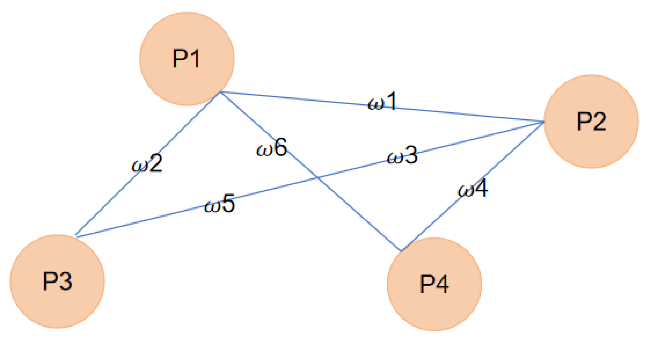
Figure 1. Two common types of system-related degradations. The first row shows turbulence degraded images under two different turbulence degrees (k), and the second row shows motion-blurred degraded images under different motion degrees.
Mathematics 12 02020 g001
Figure 2. Two common types of statistical degradations resulting from noise. The first row shows the images after Gaussian blur and the second row shows the images after Rayleigh blur.
Mathematics 12 02020 g002
Figure 3. Outline of the survey. It consists of four parts, including basic framework, categories, performance comparison, challenges, and potential direction. Specifically, categories comprise GCNs for image denoising, GCNs for image super-resolution, GCNs for image deblurring, and LLMs and GCNs for image restoration.
Mathematics 12 02020 g003
Figure 4. Social network relationship diagram. P1–4 represents different characters, and ω 1–4 represents the weight of the relationship between different characters.
Mathematics 12 02020 g004
Figure 5. Basic network framework of GCNs.
Mathematics 12 02020 g005
Figure 6. Visual illustration of the GraphSAGE sample and aggregate approach.
Mathematics 12 02020 g006
Figure 7. Visualization of GATs’ distribution of weights to different nodes.
Mathematics 12 02020 g007
Figure 8. Experimental dataset image samples. From left to right, they are Set12, BSD68, and Urban100 dataset samples.
Mathematics 12 02020 g008
Figure 9. Visual comparison of gray-scale image denoising of various methods on one sample from Urban100 with noise level σ = 25.
Mathematics 12 02020 g009
Figure 10. Visual comparisons of various methods on the SysData benchmark dataset. Models: Joint, Sharp-Shpere, Carter, and Gargoyle with the Gaussian noise of level 0.3, 0.3, and 0.3 (mean edge length).
Mathematics 12 02020 g010
Figure 11. The denoised Kinect v2 (1st row) single-frame meshes and Kinect Fusion models (2nd row).
Mathematics 12 02020 g011
Figure 12. Denoising real-scan meshes in PrintData.
Mathematics 12 02020 g012
Figure 13. Visual comparisons on Set14 datasets with ×4 scale.
Mathematics 12 02020 g013
Figure 14. Visual comparisons on Urban100 dataset with ×4 scale.
Mathematics 12 02020 g014
Table 1. Node Relationship Matrix.
P1P2P3P4
P10110
P21001
P31000
P40100
Table 2. GCNs and improved methods for image denoising.
ReferencesMethodsApplicationsKey Words (Remarks)
Shen et al. (2022) [49]GCNs3D mesh denoisingMesh Geometry, Structural Features, Graph-based Filtering
Zhao et al. (2023) [53]GCNs3D mesh denoisingGaussian curvature-driven multi-stream networks
Armando et al. (2020) [50]GCNs3D mesh denoisingGCNs for mesh denoising
Zhang et al. (2021) [43]GCNsFew-shot Learning tasks, image denoisingLDN method based on GCNs
Liu et al. (2022) [48]GATLow dose CT image denoisingEdge Enhancement Module and WGAT
Chen et al. (2021) [54]GCNsCT image denoisingEncoder-decoder-based GCNs
Chen et al. (2021) [2]GCNsLow dose CT image denoisingMulti-information fusion denoising
Jiang et al. (2023) [42]GATGraph attention denoising, synthetic noisePixel-level Features, Structure-level Features, Attention Mechanism
Mou et al. (2021) [47]GATDenoising, super-resolution, compressed sensingDynamic Attention, Graph Learning, Image Restoration
Mou et al. (2021) [46]GATDenoising, super-resolution, compressed sensingImage Restoration Using Graph Attention Networks
Chen et al. (2023) [55]GCNsDenoising method for noisy point cloudNovel geometric dual-domain GCNs for PCD
Han (2022) [45]GCNsSelf-supervised Graph DenoisingGraph Embedding, Self-supervision, Robustness
Mostafa et al. (2020) [51]GCNsGraph attention denoising, synthetic noiseAttention-based Global aggregation scheme
Li et al. (2021) [44]GCNsImage denoisingCross-patch Consistency, Long-range Dependencies, Aggregation
Table 3. GCNs combine with other methods for image denoising.
ReferencesMethodsApplicationsKey Words (Remarks)
Fu et al. (2021) [56]GCNs CNNGCNs for image De-rainingGlobal Relationship, Pixel-Channel Modeling, Fusion
Li et al. (2021) [44]GCNs CNNGCNs for image denoisingCross-patch Consistency, Patch-based Learning, Aggregation
Chen et al. (2020) [57]GCNs GANLow dose CT image denoisingNoise Distribution Learning, Non-local Self-similarity, GAN Integration
Liu et al. (2020) [58]GCNs CNNProcessing Hyperspectral Images (HSI)CNN-GCN Fusion, Spectral-Spatial Features, Hyperspectral Data
Table 4. Network optimization methods for image denoising.
ReferencesMethodsApplicationsKey Words (Remarks)
Jiang et al. (2023) [60]AGPNetImage Denoising with Graph PriorsGraph Construction, Long-distance Dependencies, k-NN Algorithm
Eliasof et al. (2021) [61]PDE-GCNsGCNs for image denoisingPartial Differential Equations, Graph Neural Networks, Over-smoothing
Hattori et al. (2022) [62]GCNsGCNs for mesh denoisingSelf-prior Learning, Vertex Position, Normal Vectors
Fu et al. (2021) [63]GCNsGCNs for image de-rainingGlobal Spatial Relationship, Inter-channel Modeling, Rain Removal
Table 5. GCNs and improved methods for image super-resolution.
ReferencesMethodsApplicationsKey Words (Remarks)
Yang et al. (2021) [64]CASGCNImage Super-ResolutionChannel Attention, Spatial Graph Convolution, Feature Enhancement
Yan et al. (2021) [65]SRGATSingle Image Super-ResolutionGraph Attention, Multi-dataset Performance, Optimization
Yang et al. (2021) [66]SGCNImage Super-ResolutionGlobal Features, Residual Refinement, Spatial Graph Attention
Zhang et al. (2021) [67]SERANsMRI Super-ResolutionMagnetic Resonance, High-resolution, Medical Imaging
Wu et al. (2019) [68]AR-GCNsPoint Cloud Super-ResolutionLocal Similarity, Point Cloud Data, Upsampling
Chen et al. (2023) [69]GCNs-MAPoint Cloud Super-ResolutionMulti-attribute, Point Cloud, Super-resolution
Liang et al. (2023) [70]MAGSRRemote Sensing Images Super-ResolutionMulti-angle, Global Features, Remote Sensing
Qian et al. (2021) [71]GCNsPoint Cloud Super-ResolutionDomain Information, Feature Extraction, Point Cloud
Zhong et al. (2023) [72]PSR-GATPoint Cloud Super-ResolutionGraph Attention, Non-local Features, Point Cloud
Cao et al. (2022) [73]GCNsVideo Captioning, Video Super-ResolutionLocal Object Relationships, Temporal Dynamics, Video Processing
Berlincioni et al. (2023) [74]4DSR-GCNs4D Video Point Cloud Upsampling4D Video, Point Cloud, Upsampling
Table 6. GCNs combine with other methods for image super-resolution.
ReferencesMethodsApplicationsKey Words (Remarks)
Zhang et al. (2021) [76]GCNs CNNImage Super-ResolutionContext-inferring, Attention Mechanism, Feature Extraction
You et al. (2022) [79]GAT CNNVideo super-resolutionMulti-scale Learning, Enhanced Attention, Temporal Dynamics
Liu et al. (2020) [58]GCNs CNNHyperspectral Image Classification, SRCNN-GCN Integration, Spectral-Spatial Features, Collaboration
Liu et al. (2023) [80]GAN GCNsFace Image Super-Resolution, InpaintingGAN-GCN Synergy, Facial Features, Generative Adversarial
Liu et al. (2023) [78]GCNs RAMRemote Sensing Images Super-ResolutionRegion-aware, Cross-block Self-similarity, Spatial Information
Zhang et al. (2023) [81]GCNs GRANElectron Microscopy Image DeblurringFully Connected Graph, Non-local Relationships, Image Quality
Table 7. Network optimization methods for image super-resolution.
ReferencesMethodsApplicationsKey Words (Remarks)
Xu et al. (2021) [82]GCNsGCNs for image super-restoration and deblurringFeature maps are converted to graph nodes
Zhang et al. (2023) [83]GCNsGCNs for image super-restorationSuper token interaction network (SPIN)
Li et al. (2022) [84]GCNsSingle Image Super-Resolution (SISR)Single Image Super-resolution Diffusion Model
Liu et al. (2020) [85]GCNsFacial expression recoveryFacial expression restoration method based on IGCN
Yue et al. (2022) [86]GCNsSpatial-temporal Video Super-resolutionSpatial-temporal Global Refinement Module (ST-GR)
Table 8. GCNs and improved methods for image deblurring.
ReferencesMethodsApplicationsKey Words (Remarks)
Liao et al. (2022) [87]GCNsDifferent types of motion image deblurringAttention mechanism, image deblur, image processing
Chen et al. (2022) [88]GCNsGCNs and GAT for image deblurringCloud removal, remote sensing image
Shen et al. (2022) [89]GCNsDeblurring of remote sensing imagesRemote sensing technology, remote sensing image processing
Li et al. (2021) [90]GCNsReal Image deblurring and super-resolutionFew-shot RealSR, Distortion Relation Graph, Transfer Learning
Table 9. GCNs combine with other methods for image deblurring.
ReferencesMethodsApplicationsKey Words (Remarks)
Li et al. (2023) [91]IFA GCNsOut-of-focus blur of the imageWavelet transform, defocus deblurring
Zhang et al. (2023) [81]GRAB GCNsImage deblurring for Low Quality (LQ) microscopy imagesMicroscopy image, image deblurring
Table 10. Network optimization methods for image deblurring.
ReferencesMethodsApplicationsKey Words (Remarks)
Liu et al. (2020) [85]GCNsFacial expression restorationFacial Expression Restoration, Generative Adversarial Network
Eliasof et al. (2021) [61]GCNsNode classification. Image deblurringAddressing Over-smoothing in GCNs
Xu et al. (2021) [82]GCNsGCNs for image super-restoration and deblurringFeature maps are converted to graph nodes
Table 11. LLMs for image restoration.
ReferencesMethodsApplicationsKey Words (Remarks)
Jin et al. [95]LLMsImage restorationCEM, Transformer (DC-former)
Wei et al. [96]LLMsImage restorationInteractive image processing
Table 12. Hyperparameters, training parameters, frameworks, and number of parameters for different models.
Model NameBatch SizeLearning RateParametersFLOPs (G)Framework
CASGCN1610−4--PyTorch
GRAN1610−43.2M145.72PyTorch
EDSR-2 × 10−438.37M6136.38PyTorch
RDN-2 × 10−421.98M3514.59PyTorch
4DSR-GCN-10−4--PyTorch
IGCN810−4---
PU-GCN640.001--PyTorch
FG-GAN100.001--TensorFlow
RGCN1610−414.5M49.75PyTorch
STSR-10−4113.3M-PyTorch
SGCN160.0114.3M-PyTorch
PSR-GAT-0.003--Torch
GRAN1610−43.2M145.72PyTorch
EDSR1610−438.37M6136.38PyTorch
RDN1610−421.98M3514.59PyTorch
Pix2pix GAN162 × 10−4---
DSen2-CR167 × 10−5---
IGCN80.0001--PyTorch
DRTL320.0001--PyTorch
RAID-Net160.001--PyTorch
WIG-Net80.9--PyTorch
GCN-Denoiser1280.001--PyTorch
ERA-WGAT1610−5--PyTorch
AGP-Net1280.01--PyTorch
GeoGCN640.001--PyTorch
DAGL321 × 10−4--PyTorch
Permutohedral-GCN----TensorFlow
DGCN101 × 10−4--TensorFlow
AdarGCN80.001--PyTorch
Table 13. PSNR (dB) of different methods on the Set12 for different noise levels (i.e., 15, 25, and 50).
DatasetsSet12
Methodsσ = 15σ = 25σ = 50
DnCNN [27]32.8630.4427.18
FFDNet [28]32.7530.4327.32
DAGL [47]33.2830.9327.81
AGP-Net [60]33.4631.1528.07
GCDN [49]33.1430.7827.60
GAiA-Net [42]33.5431.2028.18
GraphCNN [120]32.5830.1227.00
MWCNN [121]33.1530.7927.74
DRUNet [122]33.2530.4027.90
EFF-Net [123]33.3630.8127.92
Table 14. PSNR (dB) of different methods on the BSD68 for different noise levels (i.e., 15, 25, and 50).
DatasetsBSD68
Methodsσ = 15σ = 25σ = 50
DnCNN [27]31.7329.2326.23
FFDNet [28]31.6329.1926.29
DAGL [47]31.9329.4626.51
AGP-Net [60]31.0229.5926.71
GCDN [49]31.8329.3526.38
GAiA-Net [42]32.0929.6726.75
MWCNN [121]31.8829.4126.53
DRUNet [122]31.9129.4826.59
EFF-Net [123]31.9229.4926.61
Table 15. PSNR (dB) of different methods on the Urban100 for different noise levels (i.e., 15, 25, and 50).
DatasetsUrban100
Methodsσ = 15σ = 25σ = 50
DnCNN [27]32.6429.9526.23
FFDNet [28]32.4029.9026.50
DAGL [47]33.7931.3927.97
AGP-Net [60]33.8931.5128.62
GCDN [49]33.4730.9527.41
GAiA-Net [42]33.9231.6828.70
MWCNN [121]33.1730.6627.42
DRUNet [122]33.4031.1127.96
EFF-Net [123]33.7331.4528.49
Table 16. The average normal angular errors E a (from left to right) of each method in SysData.
DatasetsSysData
MethodsNoisy InputLRCNRDNFNFNGCN-D
1st row28.656.522.224.55.021.86
2nd row33.1712.178.038.348.844.39
3rd row31.787.568.727.986.895.25
Table 17. The average normal angular errors E a (from left to right) of each method in Kinect.
DatasetsKinect
MethodsNoisy InputBNFGNFCNRNFNGCD-D
1st row20.89.257.966.937.516.58
2nd row17.8912.9911.9511.9412.1511.61
Table 18. The average normal angular errors E a (from left to right) of each method in PrintData.
DatasetsPrintData
MethodsNoisy InputGNFLRCNRDNFGCN-D
1st row10.8812.0612.2711.0210.7410.54
2nd row18.0818.6817.9617.2317.6717.08
3rd row16.1616.9618.815.5315.9614.95
4th row8.087.57.976.116.685.84
Table 19. PSNR/SSIM of different methods on double scale.
MethodsScaleSet5Set14BSD100Urban100Manga109
PSNR/SSIMPSNR/SSIMPSNR/SSIMPSNR/SSIMPSNR/SSIM
Bicubic×233.66/0.929930.24/0.868829.56/0.843126.88/0.840330.80/0.9339
SRCNN [124]×236.66/0.954232.45/0.906731.36/0.887929.50/0.894635.60/0.9663
VDSR [125]×237.53/0.959033.05/0.913031.90/0.896030.77/0.914037.22/0.9750
EDSR [115]×238.11/0.960233.92/0.919532.32/0.901332.93/0.935139.10/0.9773
RCAN [126]×238.27/0.961434.11/0.921632.41/0.902633.34/0.938539.43/0.9786
NLRN [26]×238.00/0.960333.46/0.915932.19/0.899231.81/0.9246-/-
SRFBN [127]×238.11/0.960933.82/0.919632.29/0.901032.62/0.932839.08/0.9779
SAN [128]×238.31/0.962034.07/0.921332.42/0.902833.10/0.937039.32/0.9792
RDN [129]×238.24/0.961434.01/0.921232.34/0.901732.89/0.935339.18/0.9780
USRNet [130]×237.77/0.959233.49/0.915632.10/0.898131.79/0.925538.37/0.9760
HAN [131]×238.27/0.961434.16/0.921732.41/0.902733.35/0.938539.46/0.9785
SRGAT [65]×238.20/0.961033.93/0.920132.34/0.901432.90/0.935939.30/0.9785
SCET [132]×238.06/0.961533.78/0.919832.24/0.900632.38/0.929939.86/0.9821
SwinIR [133]×238.35/0.962034.14/0.921532.44/0.903033.40/0.939339.60/0.9792
RGCN [134]×238.30/0.961634.10/0.921332.44/0.903033.15/0.937739.38/0.9784
Table 20. PSNR/SSIM of different methods on triple scale.
MethodsScaleSet5Set14BSD100Urban100Manga109
PSNR/SSIMPSNR/SSIMPSNR/SSIMPSNR/SSIMPSNR/SSIM
Bicubic×330.39/0.868227.55/0.774227.21/0.738524.46/0.734926.95/0.8556
SRCNN [124]×332.75/0.909029.30/0.821528.41/0.786326.24/0.798930.48/0.9117
VDSR [125]×333.67/0.921029.78/0.832028.83/0.799027.14/0.829032.01/0.9340
EDSR [115]×334.65/0.928030.52/0.846229.25/0.809328.80/0.865334.17/0.9476
RCAN [126]×334.74/0.929930.65/0.848229.32/0.811129.09/0.870234.44/0.9499
NLRN [26]×334.27/0.926630.16/0.837429.06/0.802627.93/0.8453-/-
SRFBN [127]×334.70/0.929230.51/0.846129.24/0.808428.73/0.864134.18/0.9481
SAN [128]×334.75/0.930030.59/0.847629.33/0.811228.93/0.867134.30/0.9494
RDN [129]×334.71/0.929630.57/0.846829.26/0.809328.80/0.865334.13/0.9484
USRNet [130]×334.43/0.927930.51/0.844629.18/0.807628.38/0.857534.05/0.9466
HAN [131]×334.75/0.929930.67/0.848329.32/0.811029.10/0.870534.48/0.9500
SRGAT [65]×334.75/0.929730.63/0.847429.29/0.809928.90/0.866634.42/0.9495
RGCN [134]×334.77/0.930130.67/0.848629.33/0.811428.99/0.867934.47/0.9501
SCET [132]×334.53/0.927830.43/0.844129.17/0.807528.38/0.855934.29/0.9503
ESRT [135]×334.42/0.926830.43/0.843329.15/0.806328.46/0.857433.95/0.9455
LBNet [136]×334.47/0.927730.38/0.841729.13/0.806128.42/0.855933.82/0.9460
SwinIR [133]×334.89/0.931230.77/0.850329.37/0.812429.29/0.874434.74/0.9518
Table 21. PSNR/SSIM of different methods on quadruple scale.
MethodsScaleSet5Set14BSD100Urban100Manga109
PSNR/SSIMPSNR/SSIMPSNR/SSIMPSNR/SSIMPSNR/SSIM
Bicubic×428.42/0.810426.00/0.702725.96/0.667523.14/0.657724.89/0.7866
SRCNN [124]×430.48/0.862827.50/0.751326.90/0.710125.52/0.722127.58/0.8555
VDSR [125]×431.35/0.883028.02/0.768027.29/0.072625.18/0.754028.83/0.8870
EDSR [115]×432.46/0.896828.80/0.787627.71/0.742026.64/0.803331.02/0.9148
RCAN [126]×432.63/0.900228.87/0.788927.77/0.743626.82/0.808731.22/0.9173
NLRN [26]×431.92/0.891628.36/0.774527.48/0.734625.79/0.7729-/-
SRFBN [127]×432.47/0.898328.81/0.786827.72/0.740926.60/0.801531.15/0.9160
SAN [128]×432.64/0.900328.92/0.788827.78/0.743626.79/0.806831.18/0.9169
RDN [129]×432.47/0.899028.81/0.787127.72/0.741926.61/0.802831.00/0.9151
USRNet [130]×432.42/0.897828.83/0.787127.69/0.740426.44/0.797631.11/0.9154
HAN [131]×432.64/0.900228.90/0.789027.80/0.744226.85/0.809431.42/0.9177
SRGAT [65]×432.57/0.899728.86/0.787927.77/0.742126.76/0.805231.41/0.9181
RGCN [134]×432.65/0.900528.91/0.789227.79/0.744026.85/0.808931.24/0.9176
SCET [132]×432.27/0.896328.72/0.784727.67/0.739026.33/0.791531.10/0.9155
ESRT [135]×432.19/0.894728.69/0.783327.69/0.737926.39/0.796230.75/0.9100
LBNet [136]×432.29/0.896028.68/0.783227.62/0.738226.27/0.790630.76/0.9111
SwinIR [133]×432.72/0.902128.94/0.791427.83/0.745927.07/0.816431.67/0.9226
Table 22. PSNR/SSIM of different methods at double scale, quadruple scale and octuple scale.
MethodsScaleSet5Set14Urban100BSD100
PSNR/SSIMPSNR/SSIMPSNR/SSIMPSNR/SSIM
SRCNN [124]×236.66/0.954232.45/0.906729.50/0.894631.36/0.8879
FSRCNN [137]×237.05/0.956032.66/0.909029.88/0.902031.53/0.8920
VDSR [125]×237.53/0.959033.05/0.913030.77/0.914031.90/0.8960
RDN [129]×238.24/0.961434.01/0.921232.89/0.935332.34/0.9017
D-DBPN [138]×238.09/0.960033.85/0.919032.55/0.932432.27/0.9000
EDSR [115]×238.11/0.960233.92/0.919532.93/0.935132.32/0.9013
GCEDSR [82]×238.29/0.961534.05/0.921333.12/0.938632.39/0.9023
SRCNN×430.48/0.862827.50/0.751324.52/0.722126.90/0.7101
FSRCNN×430.72/0.866027.61/0.755024.62/0.728026.98/0.7150
VDSR×431.35/0.883028.02/0.768025.18/0.754027.29/0.7260
RDN×432.47/0.899028.81/0.787126.61/0.802827.72/0.7419
D-DBPN×432.47/0.898028.82/0.786026.38/0.794627.72/0.7400
EDSR×432.46/0.896828.80/0.787626.64/0.803327.71/0.7420
GCEDSR×432.61/0.900128.89/0.788526.72/0.807927.76/0.7439
SRCNN×825.33/0.690023.76/0.591021.29/0.544024.13/0.5660
FSRCNN×820.13/0.552019.75/0.482021.32/0.538024.21/0.5680
VDSR×825.93/0.724024.26/0.614021.70/0.571024.49/0.5830
D-DBPN×827.21/0.784025.13/0.648022.73/0.631224.88/0.6010
EDSR×826.96/0.776224.91/0.642022.51/0.622124.81/0.5985
GCEDSR×827.39/0.787625.18/0.650323.14/0.637024.92/0.6027
Disclaimer/Publisher’s Note: The statements, opinions and data contained in all publications are solely those of the individual author(s) and contributor(s) and not of MDPI and/or the editor(s). MDPI and/or the editor(s) disclaim responsibility for any injury to people or property resulting from any ideas, methods, instructions or products referred to in the content.

