
Unified Gas Kinetic Simulations of Lid-Driven Cavity Flows: Effect of Compressibility and Rarefaction on Vortex Structures

Abstract
1. Introduction
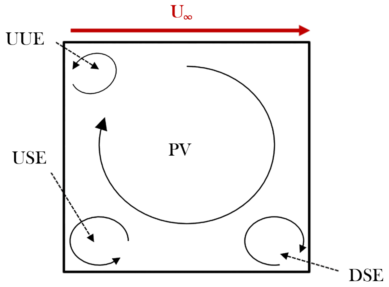
2. Vortex Dynamics in Continuum Flow Regime
3. Computational Methodology and Simulation Parameters
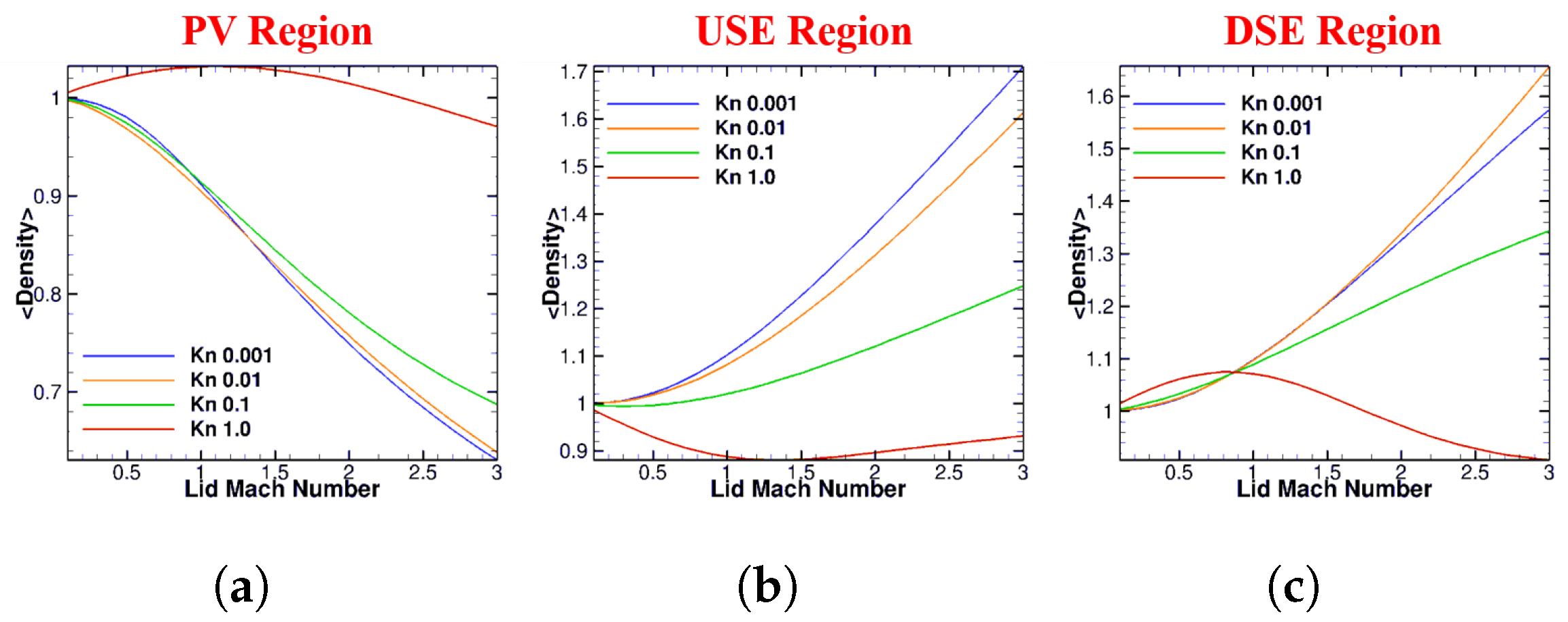
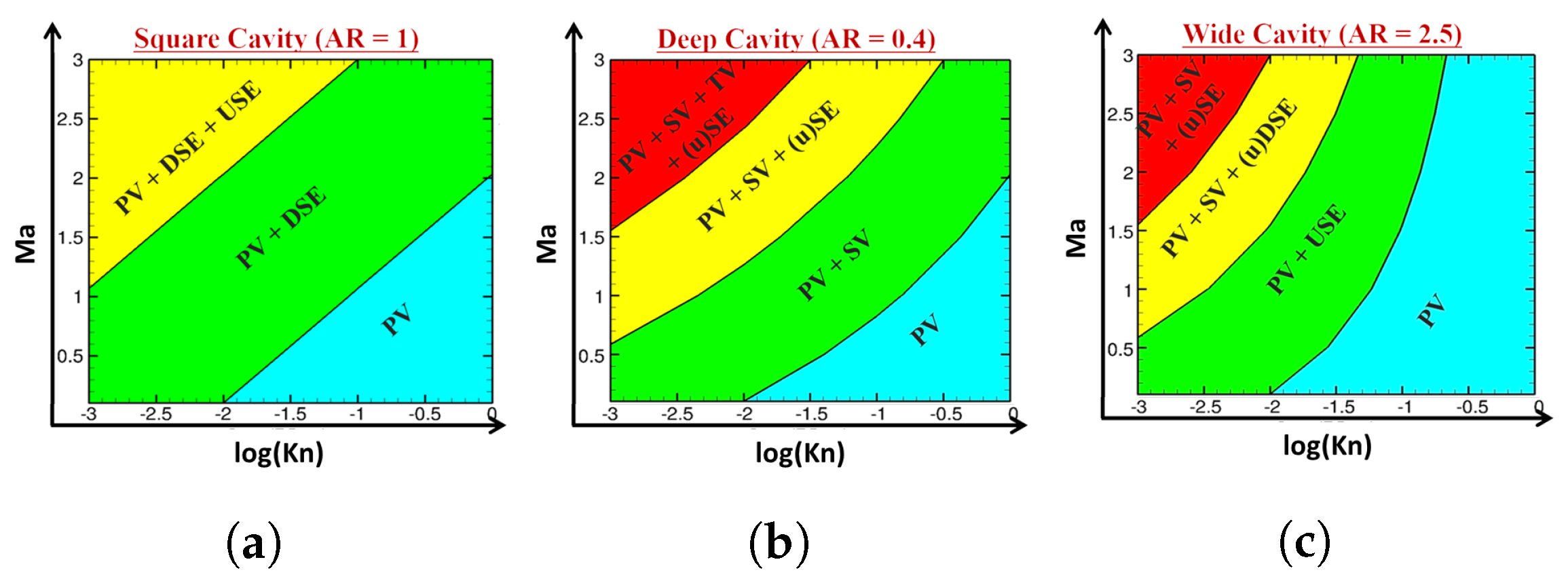
4. Flow Physics and Vortical Structures at Different and
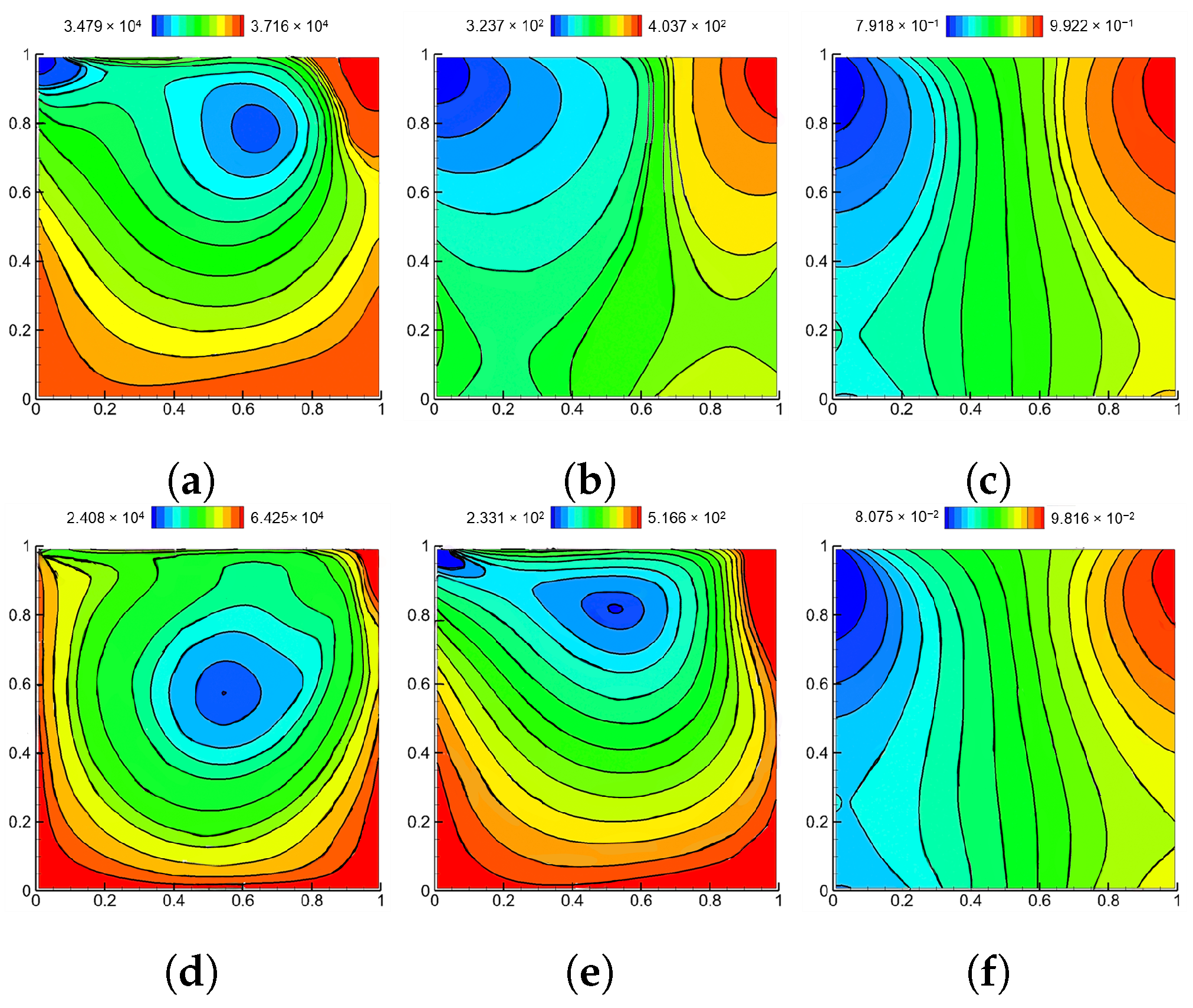
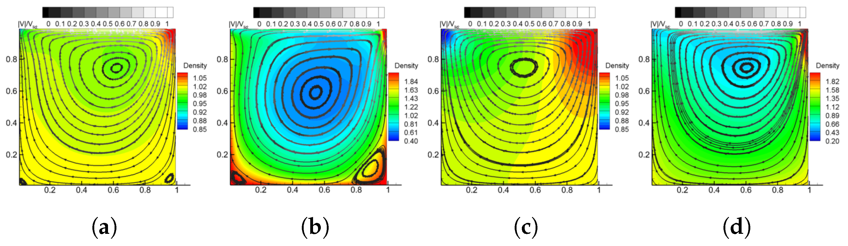
4.1. Square Cavity
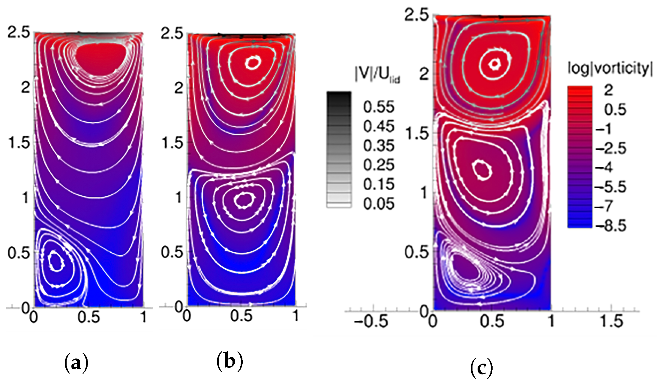
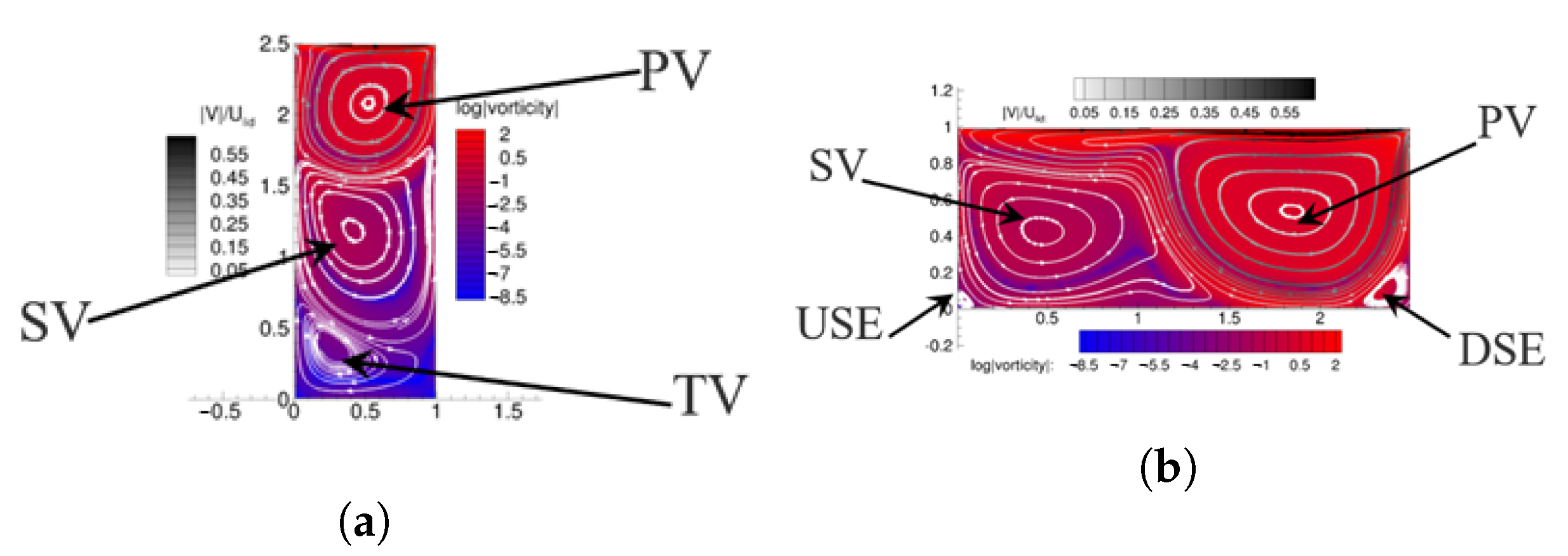
4.2. Deep Cavity
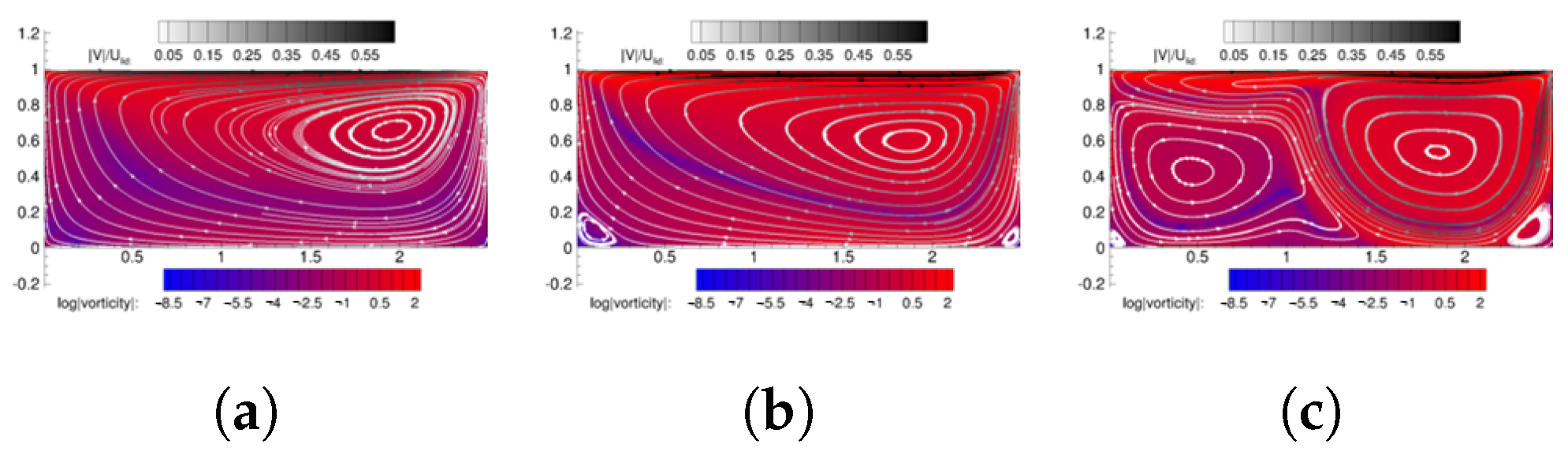
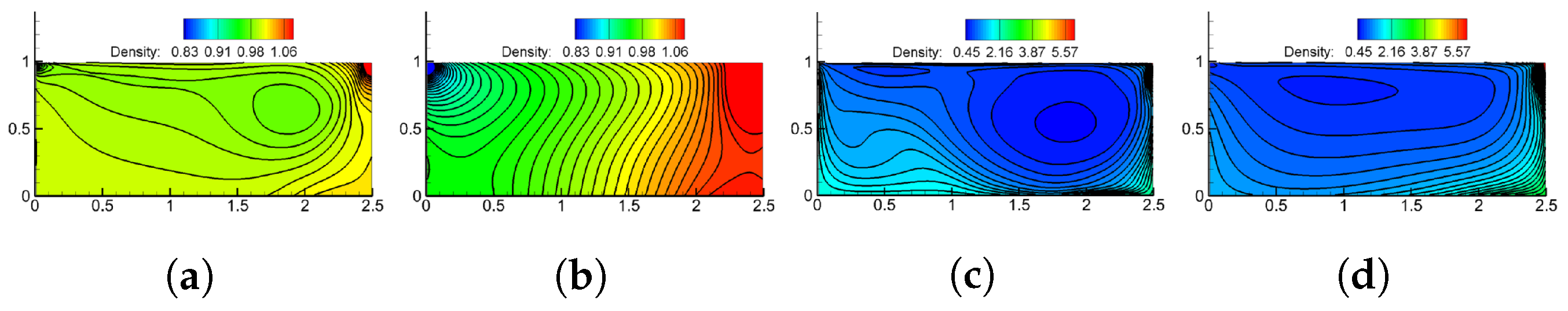
4.3. Wide Cavity
5. Conclusions
Author Contributions
Funding
Data Availability Statement
Conflicts of Interest
References
- Küchemann, D. Report on the IUTAM Symposium on Concentrated Vortex Motions in Fluids. J. Fluid Mech. 1965, 21, 1–20. [Google Scholar] [CrossRef]
- Saffman, P.G. Vortex Dynamics; Cambridge University Press: Cambridge, UK, 1995. [Google Scholar]
- Majumder, S.; Sharma, B.; Livescu, D.; Girimaji, S.S. Compressible Rayleigh—Taylor Instability Subject to Isochoric Initial Background State. Phys. Fluids 2023, 35, 094113. [Google Scholar] [CrossRef]
- Bertin, J.J.; Cummings, R.M. Critical Hypersonic Aerothermodynamic Phenomena. Annu. Rev. Fluid Mech. 2006, 38, 129–157. [Google Scholar] [CrossRef]
- Venugopal, V.; Praturi, D.S.; Girimaji, S.S. Non-Equilibrium Thermal Transport and Entropy Analyses in Rarefied Cavity Flows. J. Fluid Mech. 2019, 864, 995–1025. [Google Scholar] [CrossRef]
- He, Q.; Tao, S.; Wang, L.; Chen, J.; Yang, X. Numerical Modeling of the Heat and Mass Transfer of Rarefied Gas Flows in a Double-Sided Oscillatory Lid-Driven Cavity. Int. J. Heat Mass Transf. 2024, 230, 125788. [Google Scholar] [CrossRef]
- Zhu, M.B.; Roohi, E.; Ebrahimi, A. Computational Study of Rarefied Gas Flow and Heat Transfer in Lid-Driven Cylindrical Cavities. Phys. Fluids 2023, 35, 052012. [Google Scholar] [CrossRef]
- Nabapure, D.; Singh, A.; Kalluri, R. Investigation of Rarefied Flow Over an Open Cavity Using Direct Simulation Monte Carlo. Aeronaut. J. 2023, 127, 1009–1036. [Google Scholar] [CrossRef]
- Naris, S.; Valougeorgis, D. The Driven Cavity Flow Over the Whole Range of the Knudsen Number. Phys. Fluids 2005, 17, 097106. [Google Scholar] [CrossRef]
- Bhatnagar, P.L.; Gross, E.P.; Krook, M. A Model for Collision Processes in Gases. I. Small Amplitude Processes in Charged and Neutral One-Component Systems. Phys. Rev. 1954, 94, 511. [Google Scholar] [CrossRef]
- John, B.; Gu, X.J.; Emerson, D.R. Investigation of Heat and Mass Transfer in a Lid-Driven Cavity under Nonequilibrium Flow Conditions. Numer. Heat Transf. Part B Fundam. 2010, 58, 287–303. [Google Scholar] [CrossRef]
- Venugopal, V.; Girimaji, S.S. Unified Gas Kinetic Scheme and Direct Simulation Monte Carlo Computations of High-Speed Lid-Driven Microcavity Flows. Commun. Comput. Phys. 2015, 17, 1127–1150. [Google Scholar] [CrossRef]
- Jiang, Q.; Cai, G.; Chen, Y.; Yuan, J.; He, B.; Liu, L. Effects of Cavity Shapes and Sizes on Rarefied Hypersonic Flows. Int. J. Mech. Sci. 2023, 245, 108088. [Google Scholar] [CrossRef]
- Mousivand, M.; Roohi, E. On the Rarefied Thermally-Driven Flows in Cavities and Bends. Fluids 2022, 7, 354. [Google Scholar] [CrossRef]
- Akhlaghi, H.; Roohi, E.; Stefanov, S. Ballistic and Collisional Flow Contributions to Anti-Fourier Heat Transfer in Rarefied Cavity Flow. Sci. Rep. 2018, 8, 13533. [Google Scholar] [CrossRef] [PubMed]
- Zhu, Y.; Zhong, C.; Xu, K. GKS and UGKS for High-Speed Flows. Aerospace 2021, 8, 141. [Google Scholar] [CrossRef]
- Lokesh Kumar Ragta, B.S.; Sinha, S.S. Efficient Simulation of Multidimensional Continuum and Non-Continuum Flows by a Parallelised Unified Gas Kinetic Scheme Solver. Int. J. Comput. Fluid Dyn. 2017, 31, 292–309. [Google Scholar] [CrossRef]
- Dai, L.; Wu, H.; Tang, J. The UGKS Simulation of Microchannel Gas Flow and Heat Transfer Confined Between Isothermal and Nonisothermal Parallel Plates. J. Heat Transf. 2020, 142, 122501. [Google Scholar] [CrossRef]
- Chiang, T.; Sheu, W.; Hwang, R.R. Effect of Reynolds Number on the Eddy Structure in a Lid-Driven Cavity. Int. J. Numer. Methods Fluids 1998, 26, 557–579. [Google Scholar] [CrossRef]
- Xu, K.; Huang, J.C. A Unified Gas-Kinetic Scheme for Continuum and Rarefied Flows. J. Comput. Phys. 2010, 229, 7747–7764. [Google Scholar] [CrossRef]
- Huang, J.C.; Xu, K.; Yu, P. A Unified Gas-Kinetic Scheme for Continuum and Rarefied Flows II: Multi-Dimensional Cases. Commun. Comput. Phys. 2012, 12, 662–690. [Google Scholar] [CrossRef]
- Huang, J.C.; Xu, K.; Yu, P. A Unified Gas-Kinetic Scheme for Continuum and Rarefied Flows III: Microflow Simulations. Commun. Comput. Phys. 2013, 14, 1147–1173. [Google Scholar] [CrossRef]
- Xu, K.; Huang, J.C. An Improved Unified Gas-Kinetic Scheme and the Study of Shock Structures. IMA J. Appl. Math. 2011, 76, 698–711. [Google Scholar] [CrossRef]
- Guo, Z.; Xu, K.; Wang, R. Discrete Unified Gas Kinetic Scheme for all Knudsen number flows: Low-speed isothermal case. Phys. Rev. E 2013, 88, 033305. [Google Scholar] [CrossRef] [PubMed]
- Prendergast, K.H.; Xu, K. Numerical Hydrodynamics from Gas-Kinetic Theory. J. Comput. Phys. 1993, 109, 53–66. [Google Scholar] [CrossRef]
- Carlson, H.; Roveda, R.; Boyd, I.; Candler, G. A Hybrid CFD-DSMC Method of Modeling Continuum-Rarefied Flows. In Proceedings of the 42nd AIAA Aerospace Sciences Meeting and Exhibit, Reno, NV, USA, 5–8 January 2004; p. 1180. [Google Scholar]
- Pantazis, S.; Rusche, H. A Hybrid Continuum-Particle Solver for Unsteady Rarefied Gas Flows. Vacuum 2014, 109, 275–283. [Google Scholar] [CrossRef]
- Mohan, V.; Sameen, A.; Srinivasan, B.; Girimaji, S.S. Influence of Knudsen and Mach Numbers on Kelvin-Helmholtz Instability. Phys. Rev. E 2021, 103, 053104. [Google Scholar] [CrossRef] [PubMed]
- Karimi, M.; Girimaji, S.S. Suppression Mechanism of Kelvin-Helmholtz Instability in Compressible Fluid Flows. Phys. Rev. E 2016, 93, 041102. [Google Scholar] [CrossRef]
- Shizgal, B. A Gaussian Quadrature Procedure for Use in the Solution of the Boltzmann Equation and Related Problems. J. Comput. Phys. 1981, 41, 309–328. [Google Scholar] [CrossRef]
- Pedregosa, F.; Varoquaux, G.; Gramfort, A.; Michel, V.; Thirion, B.; Grisel, O.; Blondel, M.; Prettenhofer, P.; Weiss, R.; Dubourg, V.; et al. Scikit-Learn: Machine Learning in Python. J. Mach. Learn. Res. 2011, 12, 2825–2830. [Google Scholar]


| AR | Height | Width |
|---|---|---|
| 1.0 | 1.0 L | 1.0 L |
| 2.5 | 2.5 L | 1.0 L |
| 0.4 | 1.0 L | 2.5 L |
Disclaimer/Publisher’s Note: The statements, opinions and data contained in all publications are solely those of the individual author(s) and contributor(s) and not of MDPI and/or the editor(s). MDPI and/or the editor(s) disclaim responsibility for any injury to people or property resulting from any ideas, methods, instructions or products referred to in the content. |
© 2024 by the authors. Licensee MDPI, Basel, Switzerland. This article is an open access article distributed under the terms and conditions of the Creative Commons Attribution (CC BY) license (https://creativecommons.org/licenses/by/4.0/).
Share and Cite
Venugopal, V.; Iphineni, H.; Praturi, D.S.; Girimaji, S.S. Unified Gas Kinetic Simulations of Lid-Driven Cavity Flows: Effect of Compressibility and Rarefaction on Vortex Structures. Mathematics 2024, 12, 2807. https://doi.org/10.3390/math12182807
Venugopal V, Iphineni H, Praturi DS, Girimaji SS. Unified Gas Kinetic Simulations of Lid-Driven Cavity Flows: Effect of Compressibility and Rarefaction on Vortex Structures. Mathematics. 2024; 12(18):2807. https://doi.org/10.3390/math12182807
Chicago/Turabian StyleVenugopal, Vishnu, Haneesha Iphineni, Divya Sri Praturi, and Sharath S. Girimaji. 2024. "Unified Gas Kinetic Simulations of Lid-Driven Cavity Flows: Effect of Compressibility and Rarefaction on Vortex Structures" Mathematics 12, no. 18: 2807. https://doi.org/10.3390/math12182807
APA StyleVenugopal, V., Iphineni, H., Praturi, D. S., & Girimaji, S. S. (2024). Unified Gas Kinetic Simulations of Lid-Driven Cavity Flows: Effect of Compressibility and Rarefaction on Vortex Structures. Mathematics, 12(18), 2807. https://doi.org/10.3390/math12182807