


Fast Analysis and Optimization of a Magnetic Gear Based on Subdomain Modeling

 ,
,  ,
,  , , and
Abstract
:1. Introduction
2. Principle of Magnetic Gear
3. Subdomain Modeling
- The end effects are neglected;
- The problem is 2D in cylindrical coordinates;
- The magnetic vector potential , current density , magnetization vector , and magnetic flux density vector have the following non-zero components:
- The core materials have infinite permeability;
- The shaft is a non-magnetic material.
3.1. Governing Partial Differential Equations (PDEs)
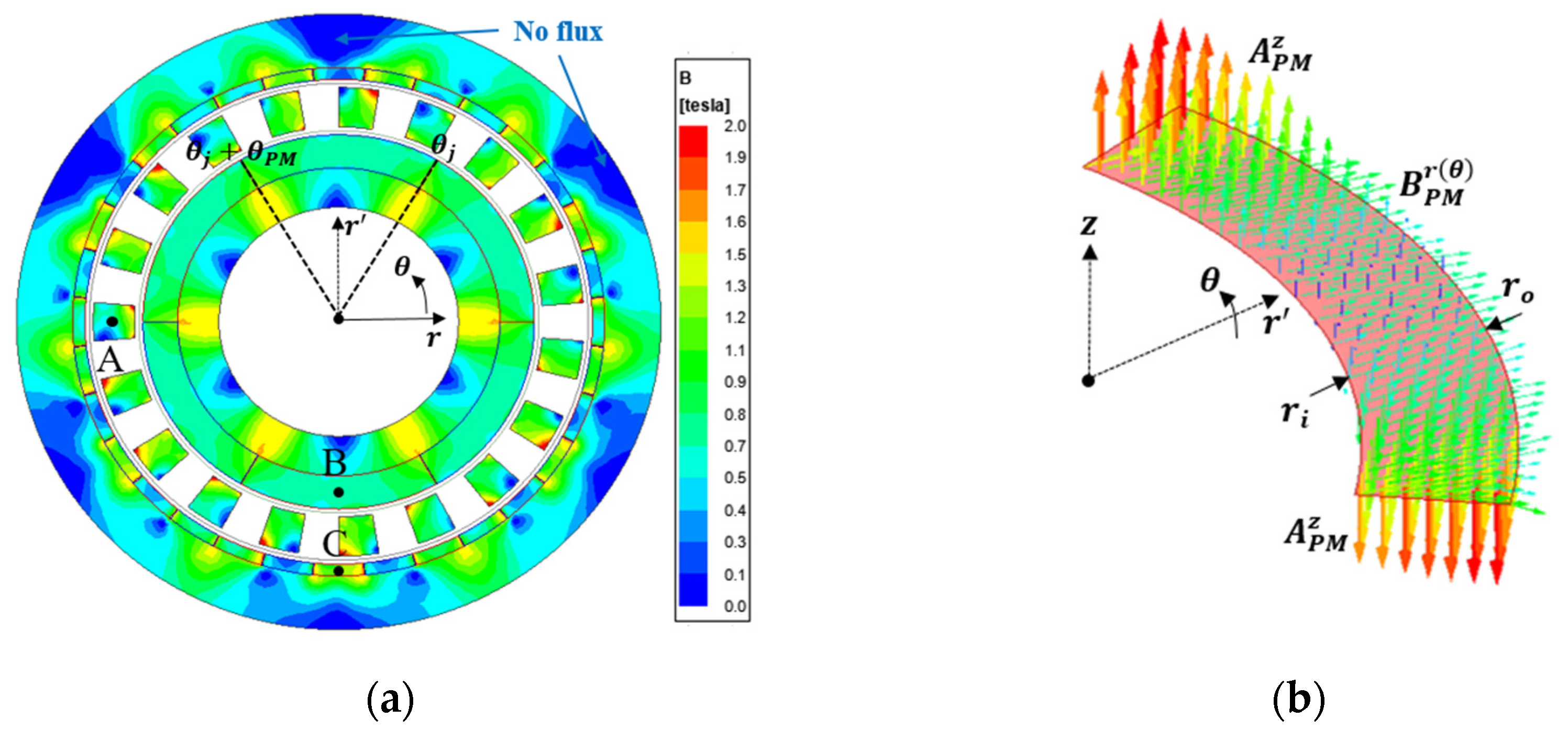
3.2. Flux Density and Improving Computational Time
4. Loss Definition
4.1. Modulation Loss
4.2. Rotor Yoke Loss
4.3. Magnet Loss
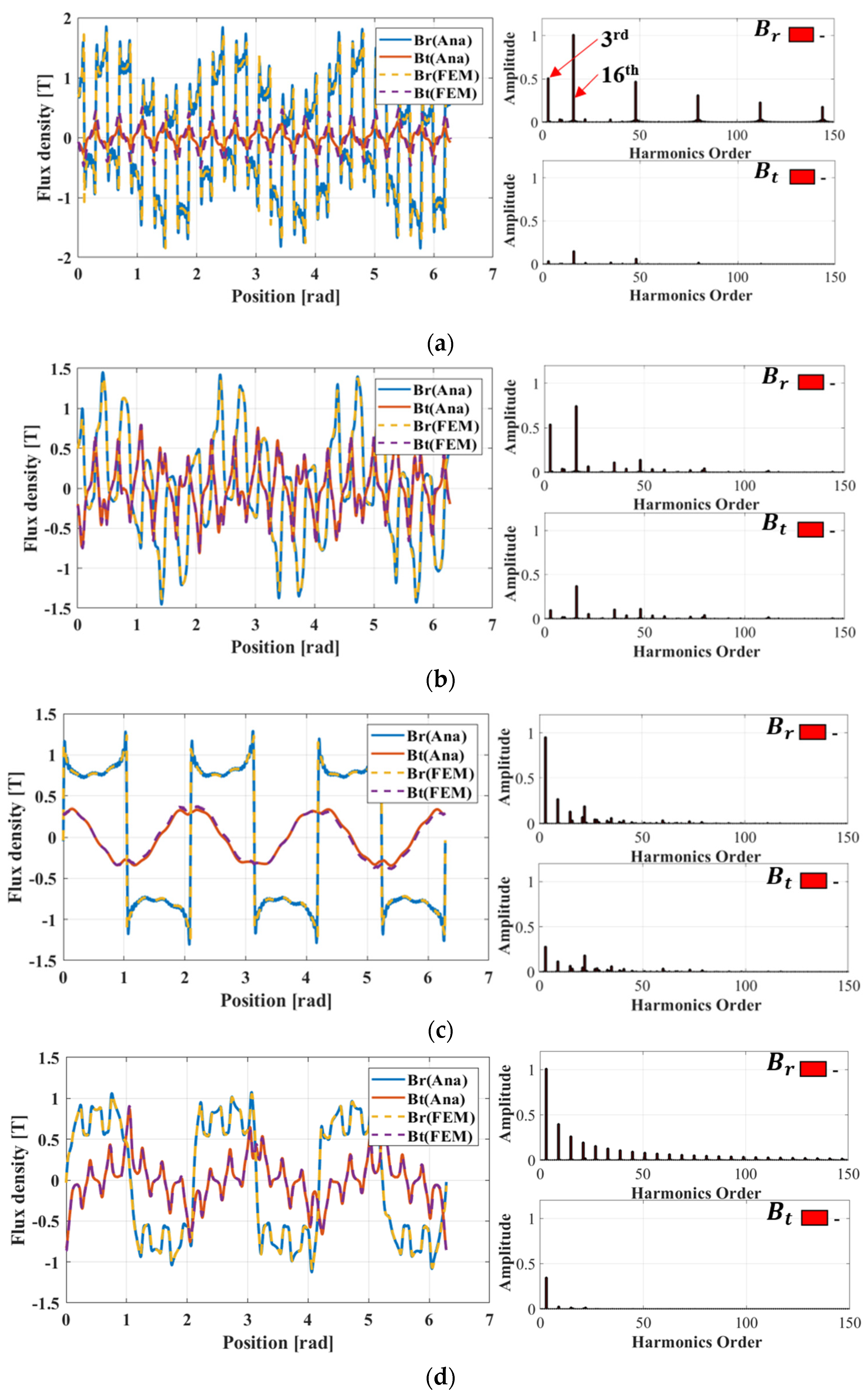
4.4. Loss Verification via FEM
- The loss of the small pole-pair combination = [11; 2] is significantly larger than that of groups [16; 3] and [17; 3] along all modulation frequency ranges. This is due to the contribution of the rotor yoke and magnet losses to the total loss. In (22) and (29), the losses depend on the rotor frequency, which is governed by the electrical frequency and pole-pair numbers in (20) and (23), respectively. Accordingly, as the number of pole pairs in the rotor decreases, the rotor frequency increases. This difference does not arise from modulation loss, as it can be attributed to the similarity of the electrical and modulation frequencies in (16).
5. Optimization Process
5.1. Variables, Objective Functions, and Constraints
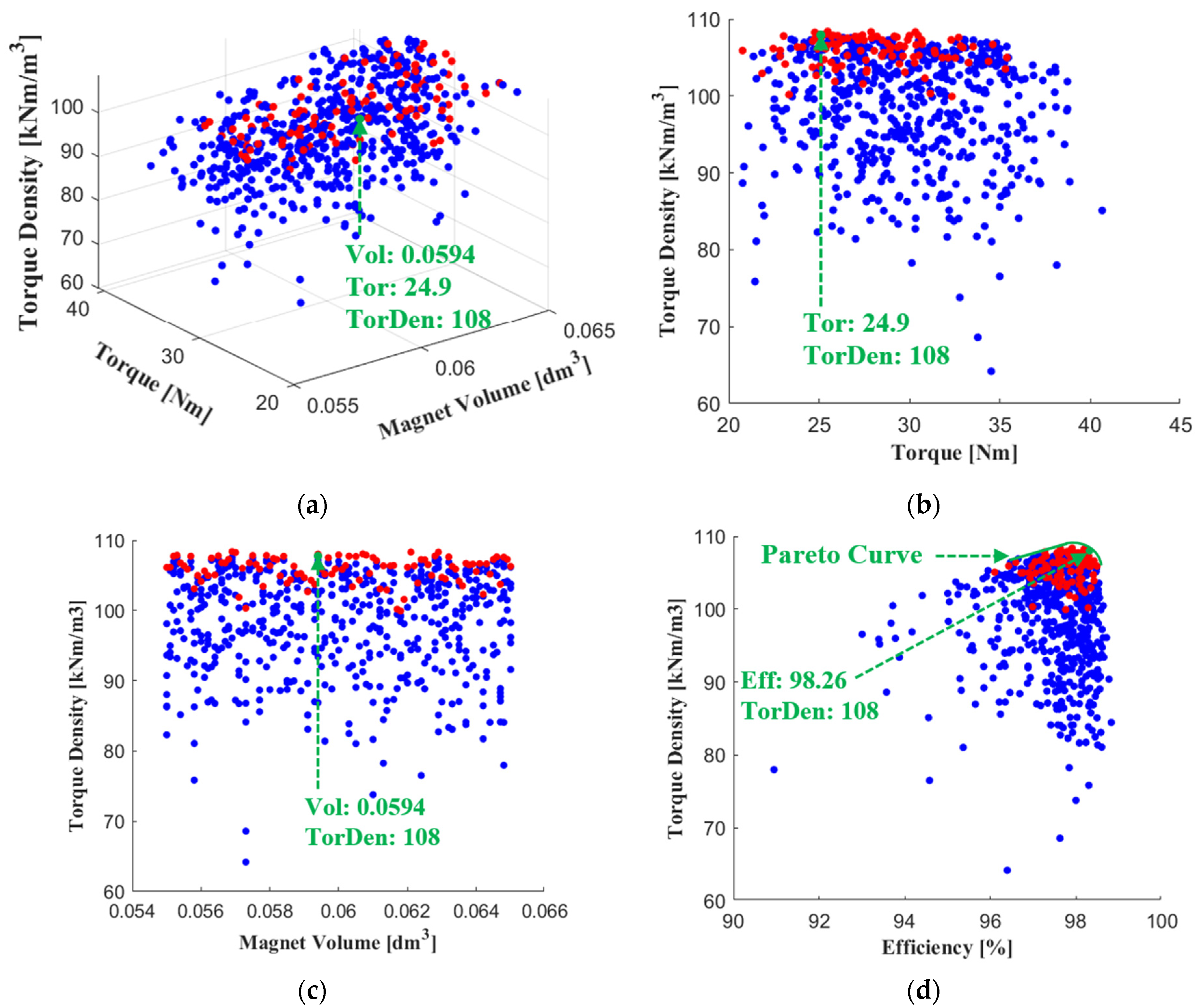
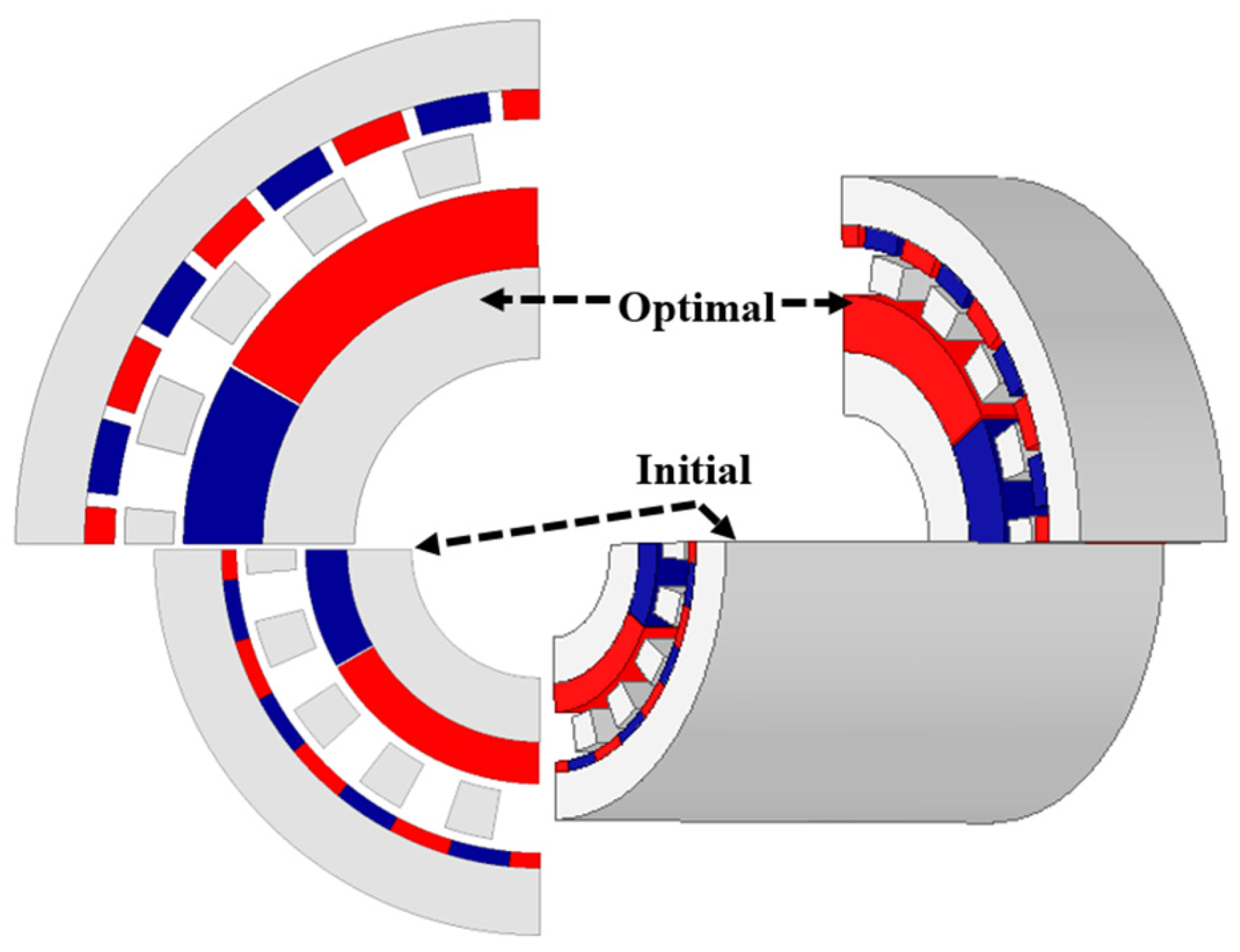
5.2. Optimization Results
6. Experimental Validation
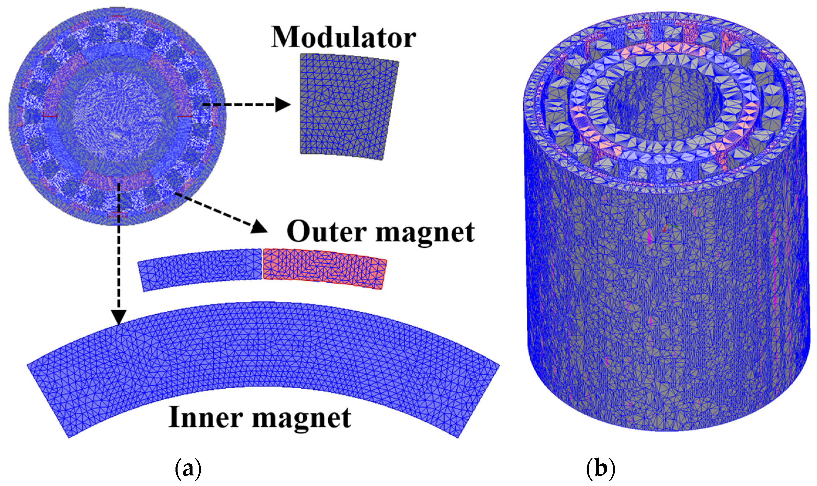
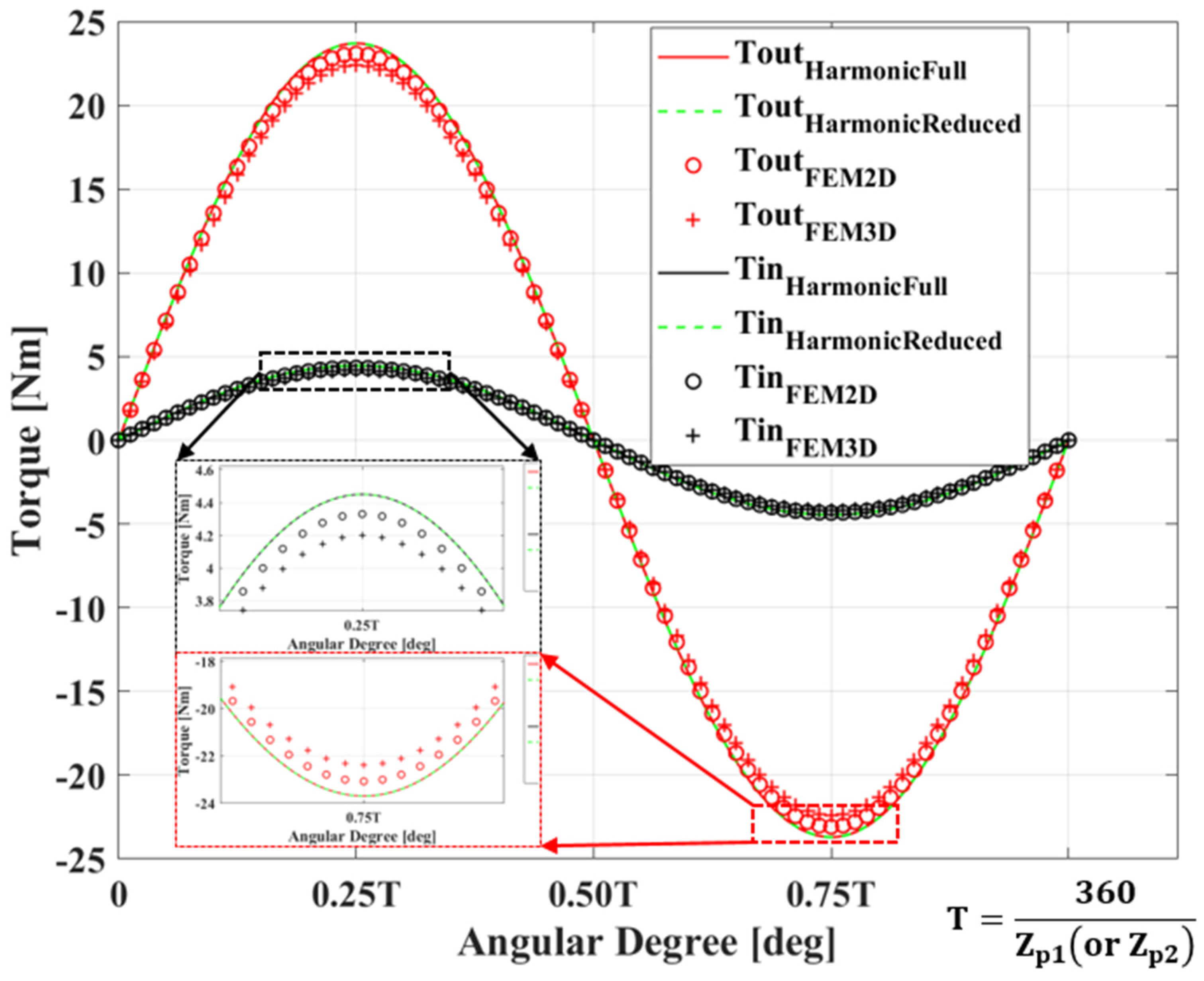
6.1. Three-Dimensional Simulation
- The harmonic reduction approach result matches that of the original analytical approach while decreasing the running time.
- Saturation occurred because of the small rotor yoke thickness, which weakened the flux linkage. Therefore, in general, the FEM produced a slightly smaller torque.
- Three-dimensional FEM was taken into account by the endcap effect. Its torque was also reduced compared with the 2D results.
- The computational times of the 2D FEM, 3D FEM, and analytical method were 4 min, more than 60 min, and 25 s, respectively. This further highlights the subdomain modeling priority.
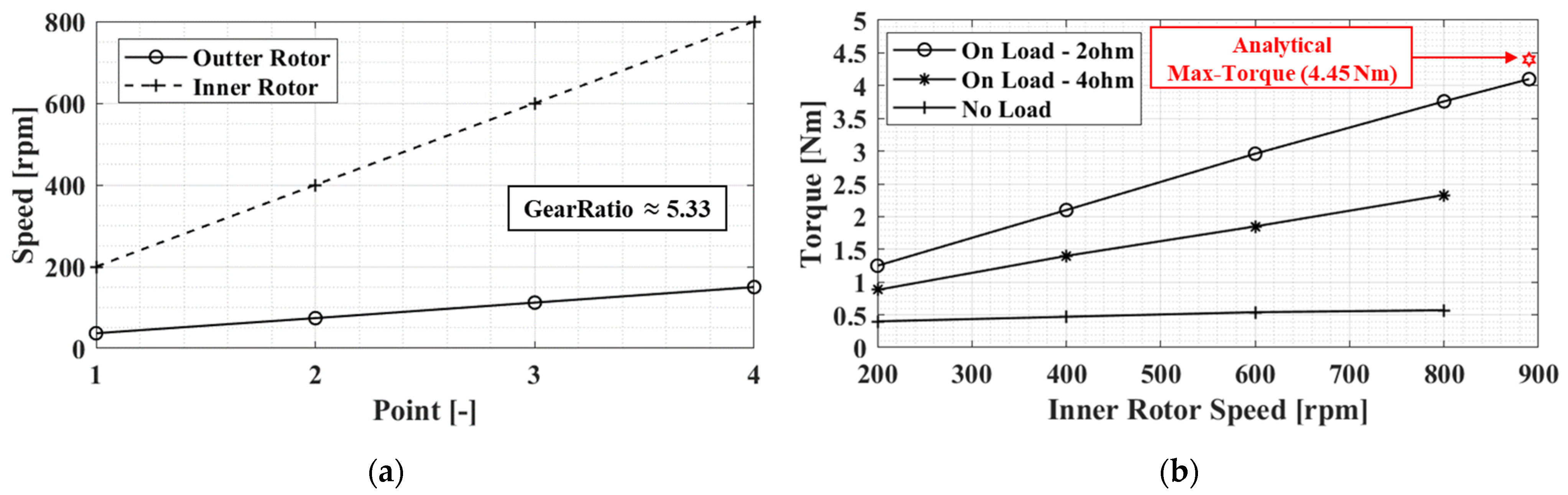
6.2. Comparison of Analysis and Experimental Results
7. Conclusions
- Consider the non-linear characteristics of magnetic materials;
- Consider the endcap effects for flux leakage prediction;
- Consider the mechanical loss in the optimization and then verify this quantity experimentally;
- Consider the demagnetization risk in the magnets.
Author Contributions
Funding
Data Availability Statement
Conflicts of Interest
References
- Martin, T. Magnetic Transmission. U.S. Patent 3 378 710, 16 April 1968. [Google Scholar]
- Atallah, K.; Howe, D. A novel high-performance magnetic gear. IEEE Trans. Magn. 2001, 37, 2844–2846. [Google Scholar] [CrossRef]
- Rasmussen, P.O.; Andersen, T.O.; Jorgensen, F.T.; Nielsen, O. Development of a high-performance magnetic gear. IEEE Trans. Ind. Appl. 2005, 41, 764–770. [Google Scholar]
- Praslicka, B.; Gardner, M.C.; Johnson, M.; Toliyat, H.A. Review and Analysis of Coaxial Magnetic Gear Pole Pair Count Selection Effects. IEEE J. Emerg. Sel. Top. Power Electron. 2022, 10, 1813–1822. [Google Scholar]
- Wang, Y.; Filippini, M.; Bianchi, N.; Alotto, P. A Review on Magnetic Gears: Topologies, Computational Models, and Design Aspects. IEEE Trans. Ind. Appl. 2019, 55, 4557–4566. [Google Scholar]
- Tlali, P.M.; Wang, R.-J.; Gerber, S. Magnetic gear technologies: A review. In Proceedings of the 2014 International Conference on Electrical Machines (ICEM), Berlin, Germany, 2–5 September 2014; pp. 544–550. [Google Scholar]
- Scheidler, J.; Asnani, V.; Tallerico, T. NASA’s magnetic gearing research for electrified aircraft propulsion. In Proceedings of the 2018 AIAA/IEEE Electric Aircraft Technologies Symposium (EATS), Cincinnati, OH, USA, 12–14 July 2018; pp. 1–12. [Google Scholar]
- Scheidler, J.; Cameron, Z.; Tallerico, T. Dynamic testing of a high-specific-torque concentric magnetic gear. In Proceedings of the Annual Forum & Technology Display—The Future of Vertical Flight, Philadelphia, PA, USA, 13–16 May 2019; pp. 1–8. [Google Scholar] [CrossRef]
- Kjaer, A.B.; Korsgaard, S.; Nielsen, S.S.; Demsa, L.; Rasmussen, P.O. Design fabrication test and benchmark of a magnetically geared permanent magnet generator for wind power generation. IEEE Trans. Energy Convers. 2020, 35, 24–32. [Google Scholar]
- Li, K.; Modaresahmadi, S.; Williams, W.B.; Wright, J.D.; Som, D.; Bird, J.Z. Designing and experimentally testing a magnetic gearbox for a wind turbine demonstrator. IEEE Trans. Ind. Appl. 2019, 55, 3522–3533. [Google Scholar]
- Li, K.; Modaresahmadi, S.; Williams, W.B.; Bird, J.Z.; Wright, J.D.; Barnett, D. Electromagnetic analysis and experimental testing of a flux focusing wind turbine magnetic gearbox. IEEE Trans. Energy Convers. 2019, 34, 1512–1521. [Google Scholar] [CrossRef]
- Wang, R.-J.; Gerber, S. Magnetically geared wind generator technologies: Opportunities and challenges. Appl. Energy 2014, 136, 817–826. [Google Scholar] [CrossRef]
- Johnson, M.; Gardner, M.C.; Toliyat, H.A.; Englebretson, S.; Ouyang, W.; Tschida, C. Design construction and analysis of a large-scale inner stator radial flux magnetically geared generator for wave energy conversion. IEEE Trans. Ind. Appl. 2018, 54, 3305–3314. [Google Scholar] [CrossRef]
- Uppalapati, K.K.; Bird, J.Z.; Jia, D.; Garner, J.; Zhou, A. Performance of a magnetic gear using ferrite magnets for low speed ocean power generation. In Proceedings of the 2012 IEEE Energy Conversion Congress and Exposition (ECCE), Raleigh, NC, USA, 15–20 September 2012; pp. 3348–3355. [Google Scholar]
- Li, W.; Chau, K.T.; Jiang, J.Z. Application of Linear Magnetic Gears for Pseudo-Direct-Drive Oceanic Wave Energy Harvesting. IEEE Trans. Magn. 2011, 47, 2624–2627. [Google Scholar] [CrossRef]
- McGilton, B.; Crozier, R.; McDonald, A.; Mueller, M. Review of magnetic gear technologies and their applications in marine energy. IET Renew. Power Gener. 2018, 12, 174–181. [Google Scholar]
- Rasmussen, P.O.; Mortensen, H.H.; Matzen, T.N.; Jahns, T.M.; Toliyat, H.A. Motor integrated permanent magnet gear with a wide torque-speed range. Proc. IEEE Energy Convers. Congr. Expo. 2009, 1510–1518. [Google Scholar]
- Rasmussen, P.O.; Frandsen, T.V.; Jensen, K.K.; Jessen, K. Experimental evaluation of a motor-integrated permanent-magnet gear. IEEE Trans. Ind. Appl. 2013, 49, 850–859. [Google Scholar]
- Frandsen, T.V.; Rasmussen, P.O.; Jensen, K.K. Improved motor intergrated permanent magnet gear for traction applications. In Proceedings of the 2012 IEEE Energy Conversion Congress and Exposition (ECCE), Raleigh, NC, USA, 15–20 September 2012; pp. 3332–3339. [Google Scholar]
- Frandsen, T.V.; Mathe, L.; Berg, N.I.; Holm, R.K.; Matzen, T.N.; Rasmussen, P.O.; Jensen, K.K. Motor integrated permanent magnet gear in a battery electrical vehicle. IEEE Trans. Ind. Appl. 2015, 51, 1516–1525. [Google Scholar] [CrossRef]
- Chmelicek, P.; Calverley, S.D.; Dragan, R.S.; Atallah, K. Dual rotor magnetically geared power split device for hybrid electric vehicles. IEEE Trans. Ind. Appl. 2019, 55, 1484–1494. [Google Scholar] [CrossRef]
- Esnoz-Larraya, J.; Valiente-Blanco, I.; Cristache, C.; Sanchez-Garcia-Casarrubios, J.; Rodriguez-Celis, F.; Diez-Jimenez, E.; Perez-Diaz, J.L. Optimagdrive: High-performance magnetic gears development for space applications. In Proceedings of the ESMATS, Hatfield, UK, 20–22 September 2017; pp. 1–5. [Google Scholar]
- Dragan, R.S.; Clark, R.E.; Hussain, E.K.; Atallah, K.; Odavic, M. Magnetically geared pseudo direct drive for safety critical applications. IEEE Trans. Ind. Appl. 2019, 55, 1239–1249. [Google Scholar] [CrossRef]
- Puchhammer, G. Magnetic gearing versus conventional gearing in actuators for aerospace applications. In Proceedings of the 42nd Aerospace Mechanism Symposium, Baltimore, MD, USA, 14–16 May 2014. [Google Scholar]
- Painter, D.S. A Comparative Study of the Performance Capabilities of Magnetic Gears. Bachelor’s Thesis, Portland State University, Portland, OR, USA, 2016. [Google Scholar]
- Jian, L.; Chau, K.T.; Li, W.; Li, J. A Novel Coaxial Magnetic Gear Using Bulk HTS for Industrial Applications. IEEE Trans. Appl. Supercond. 2010, 20, 981–984. [Google Scholar]
- Uppalapati, K.K.; Bird, J.Z.; Wright, J.; Pitchard, J.; Calvin, M.; Williams, W. A magnetic gearbox with an active region torque density of 239 Nm/L. In Proceedings of the 2014 IEEE Energy Conversion Congress and Exposition (ECCE), Pittsburgh, PA, USA, 14–18 September 2014; pp. 1422–1428. [Google Scholar]
- Kouhshahi, M.B.; Bird, J.Z.; Acharya, V.M.; Li, K.; Calvin, M.; Williams, W.; Modaresahmadi, S. An axial flux focusing magnetically geared generator for low input speed applications. IEEE Trans. Ind. Appl. 2020, 56, 138–147. [Google Scholar]
- Johnson, M.; Gardner, M.C.; Toliyat, H.A. Design and analysis of an axial flux magnetically geared generator. IEEE Trans. Ind. Appl. 2017, 53, 97–105. [Google Scholar]
- Zhu, D.; Yang, F.; Du, Y.; Xiao, F.; Ling, Z. An axial-field flux-modulated magnetic gear. IEEE Trans. Appl. Supercond. 2016, 26, 0604405. [Google Scholar] [CrossRef]
- Bomela, W.; Bird, J.Z.; Acharya, V.M. The performance of a transverse flux magnetic gear. IEEE Trans. Magn. 2014, 50, 4000104. [Google Scholar]
- RHolehouse, C.; Atallah, K.; Wang, J. A linear magnetic gear. In Proceedings of the 2012 XXth International Conference on Electrical Machines, Marseille, France, 2–5 September 2012; pp. 563–569. [Google Scholar]
- Holehouse, R.C.; Atallah, K.; Wang, J. Design and Realization of a Linear Magnetic Gear. IEEE Trans. Magn. 2011, 47, 4171–4174. [Google Scholar]
- Niu, S.; Ho, S.L.; Fu, W.N. Performance Analysis of a Novel Magnetic-Geared Tubular Linear Permanent Magnet Machine. IEEE Trans. Magn. 2011, 47, 3598–3601. [Google Scholar]
- Li, W.; Chau, K.T.; Li, J. Simulation of a Tubular Linear Magnetic Gear Using HTS Bulks for Field Modulation. IEEE Trans. Appl. Supercond. 2011, 21, 1167–1170. [Google Scholar]
- Gerber, S.; Wang, R.-J. Cogging Torque Definitions for Magnetic Gears and Magnetically Geared Electrical Machines. IEEE Trans. Magn. 2018, 54, 8103209. [Google Scholar]
- Niguchi, N.; Hirata, K. Cogging Torque Analysis of Magnetic Gear. IEEE Trans. Ind. Electron. 2012, 59, 2189–2197. [Google Scholar]
- Dai, B.; Nakamura, K.; Suzuki, Y.; Tachiya, Y.; Kuritani, K. Cogging Torque Reduction of Integer Gear Ratio Axial-Flux Magnetic Gear for Wind-Power Generation Application by Using Two New Types of Pole Pieces. IEEE Trans. Magn. 2022, 58, 8002205. [Google Scholar]
- Jungmayr, G.; Loeffler, J.; Winter, B.; Jeske, F.; Amrhein, W. Magnetic Gear: Radial Force, Cogging Torque, Skewing, and Optimization. IEEE Trans. Ind. Appl. 2016, 52, 3822–3830. [Google Scholar]
- Lubin, T.; Mezani, S.; Rezzoug, A. Analytical Computation of the Magnetic Field Distribution in a Magnetic Gear. IEEE Trans. Magn. 2010, 46, 2611–2621. [Google Scholar]
- Lubin, T.; Mezani, S.; Rezzoug, A. Development of a 2-D Analytical Model for the Electromagnetic Computation of Axial-Field Magnetic Gears. IEEE Trans. Magn. 2013, 49, 5507–5521. [Google Scholar]
- Jing, L.; Gong, J.; Ben, T. Analytical Method for Magnetic Field of Eccentric Magnetic Harmonic Gear. IEEE Access. 2020, 8, 34236–34245. [Google Scholar]
- Nguyen, M.D.; Kim, S.M.; Shin, H.S.; Shin, K.H.; Phung, A.T.; Choi, J.Y. Maximizing the output power of magnetically geared generator in low-speed applications using subdomain modeling and particle swarm optimization. AIP Adv. 2024, 14, 025117. [Google Scholar]
- Zhao, H.; Liu, C.; Song, Z.; Yu, J. A Fast Optimization Scheme of Coaxial Magnetic Gears Based on Exact Analytical Model Considering Magnetic Saturation. IEEE Trans. Ind. Appl. 2021, 57, 437–447. [Google Scholar]
- Djelloul-Khedda, Z.; Boughrara, K.; Dubas, F.; Kechroud, A.; Tikellaline, A. Analytical Prediction of Iron-Core Losses in Flux-Modulated Permanent-Magnet Synchronous Machines. IEEE Trans. Mag. 2019, 55, 6300112. [Google Scholar]
- Desvaux, M.; Sire, S.; Hlioui, S.; Ahmed, H.B.; Multon, B. Development of a Hybrid Analytical Model for a Fast Computation of Magnetic Losses and Optimization of Coaxial Magnetic Gears. IEEE Trans. Energy. Convers. 2019, 34, 25–35. [Google Scholar]
- Lee, J.I.; Shin, K.H.; Bang, T.K.; Ryu, D.W.; Kim, K.H.; Hong, K.; Choi, J.Y. Design and Analysis of the Coaxial Magnetic Gear Considering the Electromagnetic Performance and Mechanical Stress. IEEE Trans. Appl. Supercond. 2020, 30, 3700105. [Google Scholar]
- Nguyen, M.-D.; Kim, S.-M.; Lee, J.-I.; Shin, H.-S.; Lee, Y.-K.; Lee, H.-K.; Shin, K.-H.; Kim, Y.-J.; Phung, A.-T.; Choi, J.-Y. Prediction of Stress and Deformation Caused by Magnetic Attraction Force in Modulation Elements in a Magnetically Geared Machine Using Subdomain Modeling. Machines 2023, 11, 887. [Google Scholar] [CrossRef]
- Modaresahmadi, S.; Barnett, D.; Baninajar, H.; Bird, J.Z.; Williams, W.B. Structural modeling and validation of laminated stacks in magnetic gearing applications. Int. J. Mech. Sci. 2021, 192, 106133. [Google Scholar]
- Hannon, B.; Sergeant, P.; Dupré, L. Time- and Spatial-Harmonic Content in Synchronous Electrical Machines. IEEE Trans. Magn. 2017, 53, 8101011. [Google Scholar]
- Hannon, B.; Sergeant, P.; Dupré, L. Computational-Time Reduction of Fourier-Based Analytical Models. IEEE Trans. Energy Convers. 2018, 33, 281–289. [Google Scholar]
- Shin, K.-H.; Hong, K.; Cho, H.-W.; Choi, J.-Y. Core Loss Calculation of Permanent Magnet Machines Using Analytical Method. IEEE Trans. Appl. Supercond. 2018, 28, 5205005. [Google Scholar]
- Maxwell Help. Core Loss Coefficients for Electrical Steel. 2024. Available online: https://ansyshelp.ansys.com/account/secured?returnurl=/Views/Secured/Electronics/v212/en/home.htm%23../Subsystems/Maxwell/Content/CoreLossCoefficientsforElectricalSteel.htm (accessed on 1 September 2024).
- Guo, Y.G.; Zhu, J.G. Core losses in claw pole permanent magnet machines with soft magnetic composite stators. IEEE Trans. Magn. 2003, 39, 3199–3201. [Google Scholar]
- Chen, Y.; Pillay, P. An improved formula for lamination core loss calculations in machines operating with high frequency and high flux density excitation. In Proceedings of the IEEE IAS 37th Annual Meeting 2002, Pittsburgh, PA, USA, 13–18 October 2002; Volume 2, pp. 759–766. [Google Scholar]
- Cho, H.W. Characteristic Analysis of High-Speed PM Synchronous Motor Considering Power Losses and SVPWM Inverter. Ph.D. Dissertation, Chungnam National University, Daejeon, Republic of Korea, 2007. [Google Scholar]


| Quantity | Symbol | Unit | Value |
|---|---|---|---|
| Outer rotor radius | mm | 39.0 | |
| Outer external magnet radius | mm | 32.2 | |
| Inner external magnet radius | mm | 30.7 | |
| Outer modulation radius | mm | 29.7 | |
| Inner modulation radius | mm | 24.7 | |
| Outer internal magnet radius | mm | 23.7 | |
| Inner internal magnet radius | mm | 19.5 | |
| Inner rotor radius | mm | 10.0 | |
| Stack length | mm | 77.0 | |
| Remanent of magnets | T | 1.25 | |
| Magnet relative permeability | - | 1.03 | |
| Vacuum permeability | |||
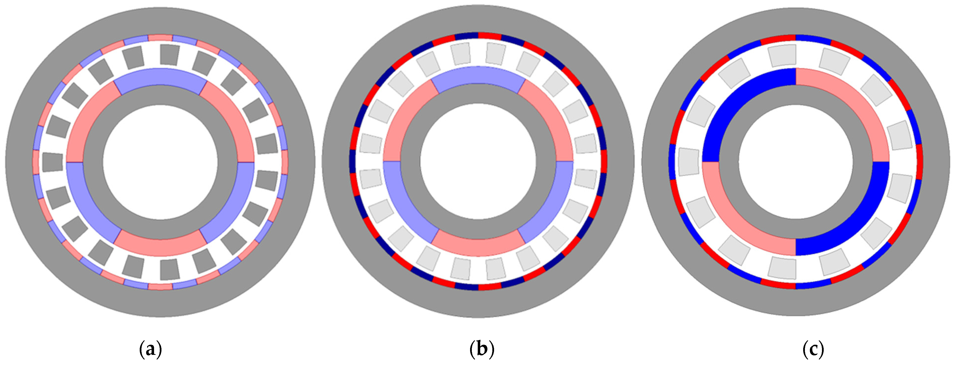
| Outer magnet pole pair | - | 11/16/17 | |
| Inner magnet pole pair | - | 2/3/3 | |
| Modulation pole | - | 13/19/20 | |
| Outer magnet pitch ratio | - | 1.0 | |
| Inner magnet pitch ratio | - | 1.0 | |
| Modulation pitch | rad | 0.5 |
| Quantity | Symbol | Unit | Value |
|---|---|---|---|
| Outer magnet pitch ratio | - | 0.7–1.0 | |
| Inner magnet pitch ratio | - | 0.7–1.0 | |
| Modulation pitch | rad | 0.4–0.6 | |
| Outer diameter | mm | 23–100 | |
| Outer magnet width | mm | 0.75–3 | |
| Modulation width | mm | 2.5–10.0 | |
| Inner magnet width | mm | 2.0–8.0 |
| Quantity | Symbol | Unit | Initial | Optimal |
|---|---|---|---|---|
| Outer rotor radius | mm | 39.0 | 53.0 | |
| Outer external magnet radius | mm | 32.2 | 46.0 | |
| Inner external magnet radius | mm | 30.7 | 43.0 | |
| Outer modulation radius | mm | 29.7 | 42.0 | |
| Inner modulation radius | mm | 24.7 | 37.0 | |
| Outer internal magnet radius | mm | 23.7 | 36.0 | |
| Inner internal magnet radius | mm | 19.5 | 28.0 | |
| Inner rotor radius | mm | 10.0 | 18.7 | |
| Stack length | mm | 77.0 | 25.6 | |
| Outer magnet pitch ratio | - | 1.00 | 0.84 | |
| Inner magnet pitch ratio | - | 1.00 | 1.00 | |
| Modulation pitch | rad | 0.50 | 0.53 |
| Characteristic | Initial Design | Optimal Design | ||
|---|---|---|---|---|
| Subdomain | FEM | Subdomain | FEM | |
| Torque—Nm | 23.7 | 23.4 | 24.9 | 24.3 |
| Torque density—kNm/m3 | 64 | 64 | 108 | 108 |
| Magnet volume—dm3 | 66.1 | 66.1 | 54.9 | 59.4 |
| Total loss—W | 10.04 | 10.39 | 13.66 | 13.65 |
| Efficiency—% | 98.67 | 98.61 | 98.26 | 98.26 |
Disclaimer/Publisher’s Note: The statements, opinions and data contained in all publications are solely those of the individual author(s) and contributor(s) and not of MDPI and/or the editor(s). MDPI and/or the editor(s) disclaim responsibility for any injury to people or property resulting from any ideas, methods, instructions or products referred to in the content. |
© 2024 by the authors. Licensee MDPI, Basel, Switzerland. This article is an open access article distributed under the terms and conditions of the Creative Commons Attribution (CC BY) license (https://creativecommons.org/licenses/by/4.0/).
Share and Cite
Nguyen, M.-D.; Jung, W.-S.; Hoang, D.-T.; Kim, Y.-J.; Shin, K.-H.; Choi, J.-Y. Fast Analysis and Optimization of a Magnetic Gear Based on Subdomain Modeling. Mathematics 2024, 12, 2922. https://doi.org/10.3390/math12182922
Nguyen M-D, Jung W-S, Hoang D-T, Kim Y-J, Shin K-H, Choi J-Y. Fast Analysis and Optimization of a Magnetic Gear Based on Subdomain Modeling. Mathematics. 2024; 12(18):2922. https://doi.org/10.3390/math12182922
Chicago/Turabian StyleNguyen, Manh-Dung, Woo-Sung Jung, Duy-Tinh Hoang, Yong-Joo Kim, Kyung-Hun Shin, and Jang-Young Choi. 2024. "Fast Analysis and Optimization of a Magnetic Gear Based on Subdomain Modeling" Mathematics 12, no. 18: 2922. https://doi.org/10.3390/math12182922
APA StyleNguyen, M.-D., Jung, W.-S., Hoang, D.-T., Kim, Y.-J., Shin, K.-H., & Choi, J.-Y. (2024). Fast Analysis and Optimization of a Magnetic Gear Based on Subdomain Modeling. Mathematics, 12(18), 2922. https://doi.org/10.3390/math12182922