Abstract
Metal–oxide–semiconductor field-effect transistors (MOSFETs) are critical in power electronic modules due to their high-power density and rapid switching capabilities. Therefore, effective thermal management is crucial for ensuring reliability and superior performance. This study used finite element analysis (FEA) to evaluate the electro-thermal behavior of MOSFETs with copper clip bonding, showing a significant improvement over aluminum wire bonding. The aluminum wire model reached a maximum temperature of 102.8 °C, while the copper clip reduced this to 74.6 °C. To further optimize the thermal performance, Latin Hypercube Sampling (LHS) generated diverse design points. The FEA results were used to select the Kriging regression model, chosen for its superior accuracy (MSE = 0.036, R2 = 0.997, adjusted R2 = 0.997). The Kriging model was integrated with a Genetic Algorithm (GA), further reducing the maximum temperature to 71.5 °C, a 4.20% improvement over the original copper clip design and a 43.8% reduction compared to aluminum wire bonding. This integration of Kriging and the GA to the MOSFET copper clip package led to a significant improvement in the heat dissipation and overall thermal performance of the MOSFET package, while also reducing the computational power requirements, providing a reliable and efficient solution for the optimization of MOSFET copper clip packages.
Keywords:
MOSFETs; thermal management; copper clip bonding; finite element analysis; Latin hypercube sampling; kriging model; genetic algorithm; optimization MSC:
90C31
1. Introduction
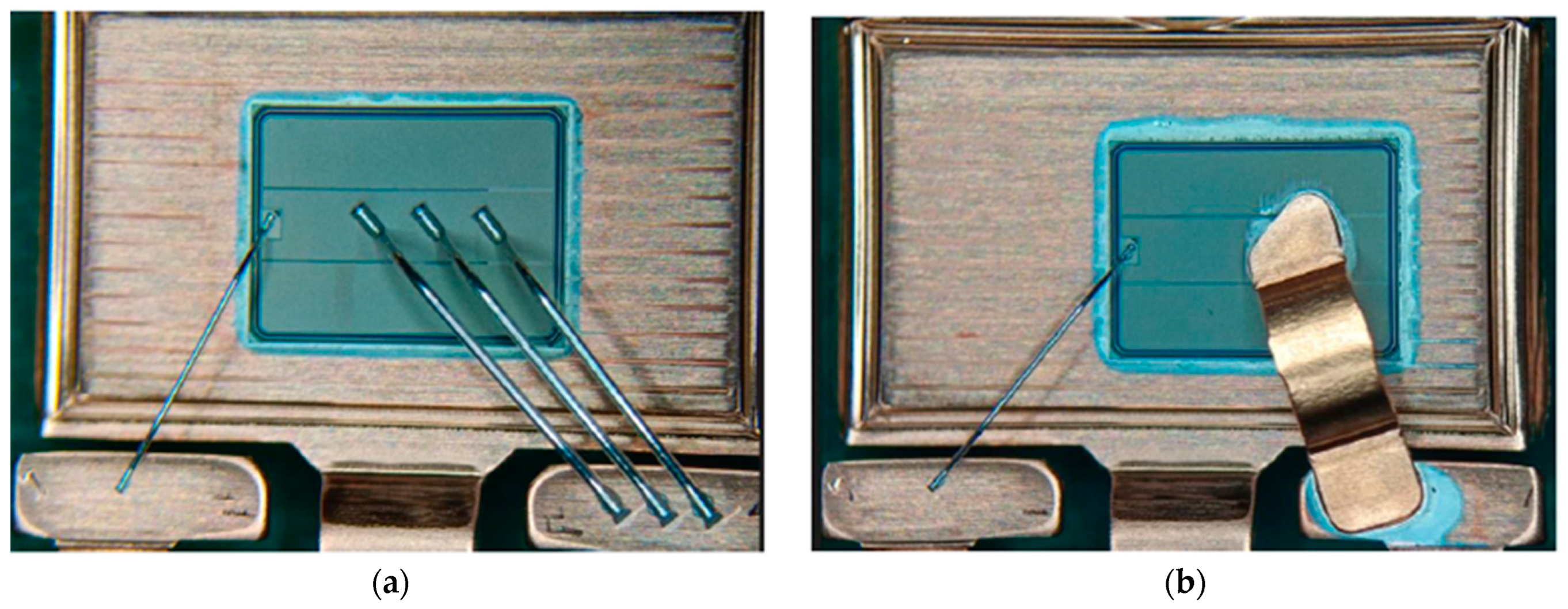
Due to their fast-switching speed and high-power density, metal–oxide–semiconductor field-effect transistors (MOSFETs) are essential components of power electronic modules. They are important in many high-performance electronic applications, such as industrial and automotive systems [1,2]. However, in regard to these semiconductors, heat loss caused by electrical resistance leads to energy consumption issues and is a major cause of semiconductor failure, which can severely compromise the performance and longevity of entire electronic systems, particularly in high-power and demanding environments [3]. Therefore, managing the thermal performance of semiconductors remains a critical challenge in power electronics. In MOSFET packaging, aluminum wire bonding has traditionally been widely used for its mechanical stability; however, it exhibits notable limitations in terms of electrical resistance and heat dissipation efficiency [4]. Over the past few years, copper clip bonding has emerged as a promising alternative, offering superior electrical and thermal conductivity, compared to aluminum wire bonding [5]. Leveraging the high electrical and thermal conductivity of copper, this method reduces both electrical and thermal resistance, thereby enhancing the switching performance of MOSFETs [6]. Figure 1 shows the aluminum wire bonding and the copper clip bonding in the TO247 MOSFET package. Furthermore, copper clips are attached to the flat die surface, making it easier to include an extra heat sink and allowing more effective thermal control [7,8]. For example, a comparison of copper clip bonding and aluminum wire bonding in a 1200 V/150 A IGBT module revealed that copper clip bonding reduced the thermal resistance by up to 23% at single semiconductor die junctions and by 18% during a parallel operation [9]. Finite element analysis (FEA) of the thermal and electrical properties of a TO247 module with a 1700 V/58 A SiC MOSFET, employing various bonding methods and materials, demonstrated that copper clip bonding effectively lowers the temperatures, even with low thermal conductivity substrates, and maintains superior performance after 100 thermal cycles [10]. Despite the recognized advantages of copper clip bonding, there remains a significant gap in the literature regarding the precise optimization of copper clip dimensions, which is crucial for maximizing the thermal management efficiency in MOSFET packages. This study addresses that gap by employing advanced computational tools to systematically optimize these dimensions.

Figure 1.
Picture of the TO247 MOSFET package: (a) aluminum wire bonding package; (b) copper clip bonding package.
Surrogate-based optimization (SBO) is a vital method to resolve intricate and computationally demanding optimization issues. This approach leverages surrogate models to approximate the behavior of expensive-to-evaluate functions, thereby significantly reducing the computational cost of optimization processes [11,12,13]. Surrogate models, often constructed using machine learning techniques, provide a cheaper and faster alternative to direct function evaluations, which are typically required in high-fidelity simulations [14,15]. Common surrogate models used in SBO include Kriging, also known as Gaussian process regression, radial basis function, and polynomial chaos expansion. Each offers distinct advantages in terms of flexibility, interpretability, and computational efficiency [16,17]. Recent advancements in SBO have demonstrated its applicability across various domains. For example, aerodynamic design optimization of a tailless Unmanned Combat Aerial Vehicle (UCAV) achieved a 15.9% objective function improvement with variable-fidelity optimization. Low-fidelity analysis overestimated the lift-to-drag ratio by (3–5)%, while the variable-fidelity results matched the high-fidelity analysis [18]. Similarly, in the field of Structural Health Monitoring (SHM), SBO techniques have been integrated with deep learning to optimize sensor placements for high-precision digital twins, enhancing the reliability and robustness of structural assessments [19].
Kriging is one of the most used methods in SBO, in comparison to other surrogate models, including those based on machine learning and deep learning techniques [20,21]. It can model complex, non-linear relationships more accurately than traditional machine learning models, such as linear and polynomial regression, as it does not require pre-specified functional forms, making it more adaptable to underlying data structures [22]. Kriging’s capacity to quantify the uncertainty in its predictions is one of its key advantages. This helps with optimization by enabling more knowledgeable search space exploration [23,24,25]. Kriging’s ability to adaptively refine its model based on new data points makes it superior to models like support vector machines (SVMs) and neural networks in regard to iterative optimization processes, ensuring increased accuracy in regions of interest [26,27,28]. Even though deep learning models are capable of high accuracy, training them requires large datasets, which necessitates substantial computer resources. On the other hand, Kriging is more appropriate for situations where computing efficiency is critical, since it offers comparable accuracy at a lower computational cost [29,30,31].
Furthermore, Kriging is a good fit for integration with Genetic Algorithms (GAs), which are often used to combine precise modeling with the powerful search capabilities of GAs to improve the efficiency of the optimization process [32]. Several studies have shown that integrating Kriging and GAs greatly increases the efficiency of the optimization process. For example, ref. [33] determined the gripping point configuration for sheet metal parts through a two-stage optimization process; this process utilized the finite element method (FEM) to analyze the mechanical properties and a GA combined with Kriging to optimize the grasping point layouts, achieving precise and efficient solutions. Similarly, ref. [34] focused on updating structural dynamic models based on acceleration frequency response functions using FEA, Kriging, and a GA, which improved the reliability and accuracy of the models, crucial to predicting and mitigating structural failures. Furthermore, ref. [35]’s research on evolutionary black-box topology optimization employs a GA and Kriging models analyzed using FEA to address complex topology optimization problems, demonstrating the effective handling of high-dimensional design spaces. Reference [36] combines Kriging surrogate models with a GA to design curvilinearly stiffened plates; FEA is used to validate the designs to optimize the vibration and buckling resistance, resulting in more robust and efficient structural designs. Additionally, ref. [37] discusses a technique combining FEA, constrained Latin Hypercube Sampling (LHS), and genetic programming, which enhances the efficiency and accuracy of the optimization process. These studies emphasize how effective FEA, Kriging, and GAs work together to optimize challenging engineering issues.
Inspired by the substantial literature demonstrating the promising performance of surrogate models in thermal management applications, the primary goal of this research is to address the gap in the use of advanced computational tools to optimize thermal management in the TO247 MOSFET package. This study employed a surrogate-based optimization approach, utilizing the Kriging–GA optimization process, due to its proven efficiency in handling complex, non-linear design spaces. By integrating these methods, this research aims to achieve a more precise and computationally efficient optimization of copper clip sizes, directly improving the thermal management of MOSFETs. The optimization process then began with FEA simulations to compare the thermal performance of MOSFETs with aluminum wire bonding and copper clip bonding. The initial designs for the copper clip bonding parameters were generated using LHS, which provided a diverse set of design points for the subsequent FEA simulations. The results from these simulations formed the dataset used to train and test the Kriging surrogate model, which accurately approximates the thermal behavior of the MOSFET with copper clips. The Kriging surrogate model was then utilized as the objective function in the optimization process. The flexibility and accuracy of this model in capturing complex, non-linear relationships made it particularly suitable for this application. A GA was employed to navigate the design space efficiently and identify the optimal copper clip size. The GA was chosen for its robust search mechanisms, adaptability, and effectiveness in handling multi-objective and constrained optimization problems. Various constraints, such as geometric and thermal performance limits, were incorporated into the GA to ensure feasible and practical design solutions. By integrating the Kriging surrogate model with the GA, this study conducted an efficient and comprehensive search for the optimal copper clip design. This approach demonstrates a reduction in computational costs through the use of surrogate models, while also setting a precedent for future optimization studies in power electronics.
2. The Proposed Design Optimization Framework
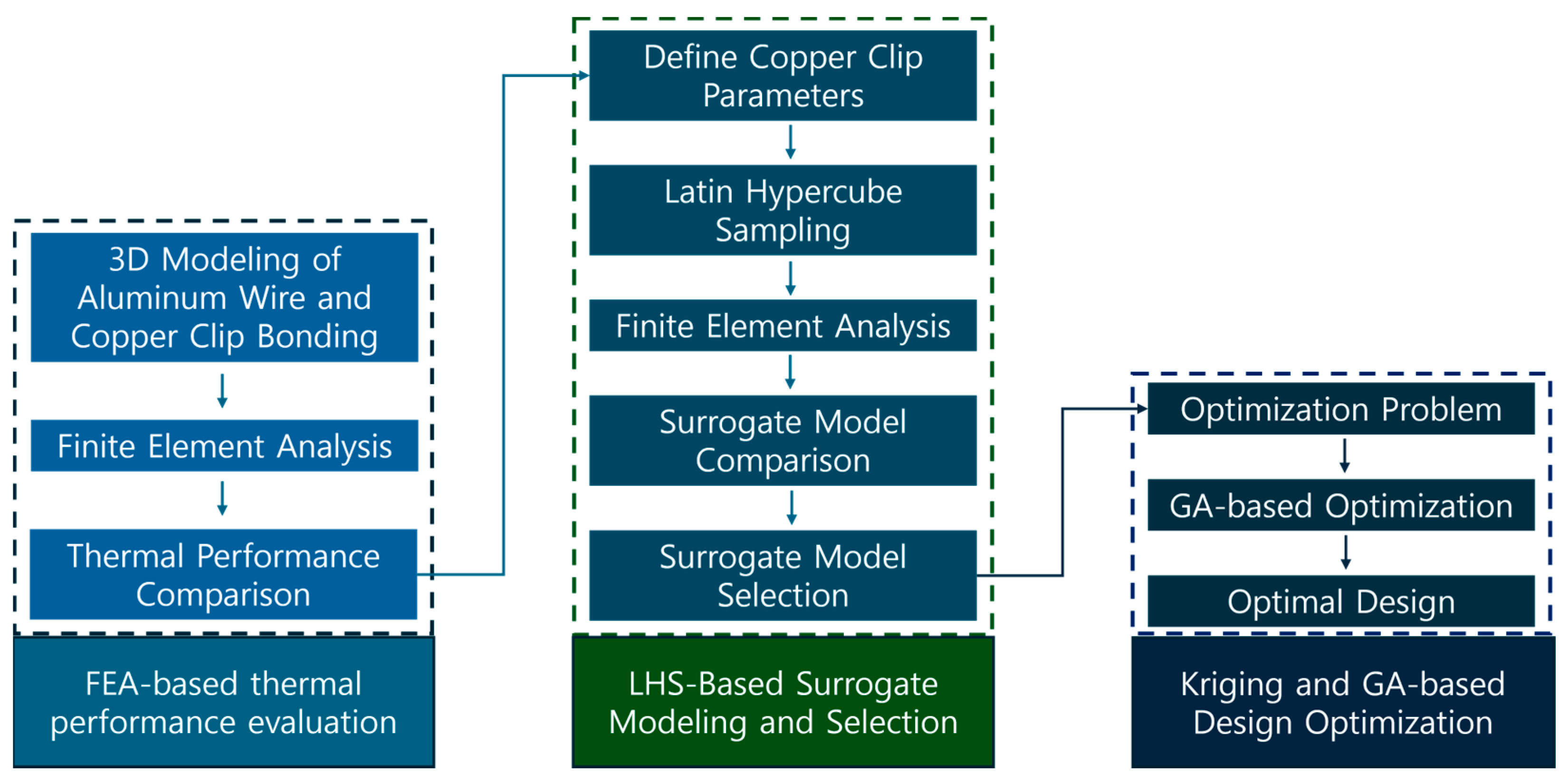
This section outlines the comprehensive approach used to optimize the copper clip size for MOSFETs, aimed at enhancing thermal management. Figure 2 shows the comprehensive methodology used to optimize the copper clip size for MOSFETs to enhance the thermal management. The framework is systematically designed to ensure a thorough exploration of the design space and to achieve the best possible thermal performance. The process begins with the 3D modeling of aluminum wire and copper clip bonding configurations. FEA is then conducted to compare their thermal performance, providing essential insights into the temperature distribution and heat dissipation across the MOSFET package. This initial analysis forms the basis for the FEA-based thermal performance evaluation. Subsequently, the copper clip parameters are defined and LHS is employed to generate a diverse set of design points to ensure a thorough exploration of the design space. These sampled points undergo FEA to evaluate their thermal performance, while the results are used for surrogate model training and performance evaluation.
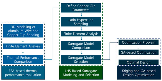
Figure 2.
Comprehensive optimization methodology for copper clip size in MOSFETs using FEA, LHS, and a Kriging surrogate model, assisted by a GA.
Among the surrogate models evaluated, the Kriging model is selected for its superior accuracy in predicting thermal behavior. The model is then integrated into a GA-based optimization framework, which is specifically designed to efficiently explore the design space, while adhering to defined constraints. The optimization problem is formulated, incorporating the necessary constraints, and the GA is employed to perform evolutionary operations, iteratively refining the design parameters. Through this iterative optimization process, the optimal copper clip design is identified, leading to significant improvements in thermal management. Figure 2 shows a flow chart of this optimization framework, illustrating the key steps, from the generation of design points via LHS, through surrogate model training and selection, to the final GA-driven optimization that determines the optimal copper clip dimensions.
2.1. Finite Element Analysis
This study employed FEA to simulate and evaluate the electro-thermal performance of MOSFETs with different bonding techniques, specifically comparing traditional aluminum wire bonding and advanced copper clip bonding. To address the optimization problem, parameters related to copper clip bonding were selected and the simulation results were generated using a Latin Hypercube Sampling (LHS) approach within the framework of the Design of Experiments (DoEs).
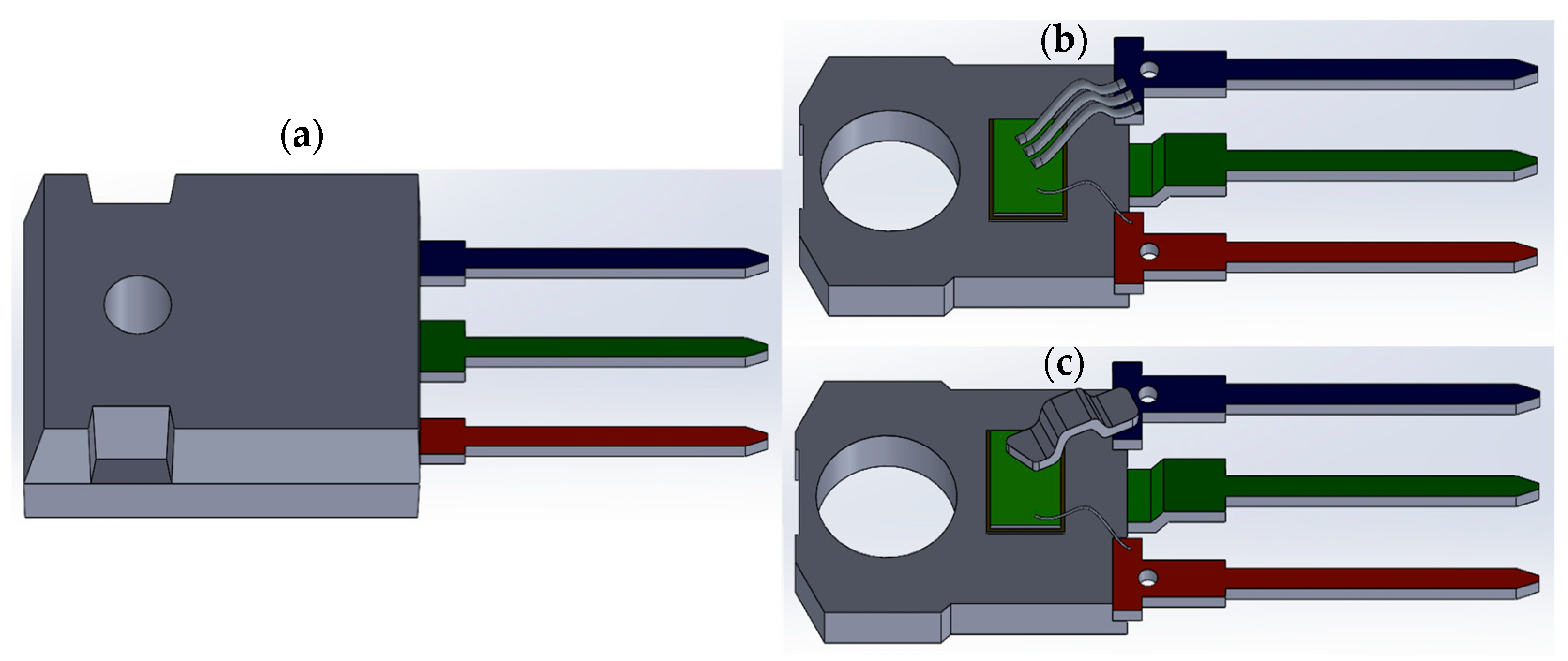
The Computer-Aided Design (CAD) for both the aluminum wire bonding and copper clip bonding models for the TO247 MOSFET package were developed using SOLIDWORKS [38]. Figure 3 illustrates the CAD models created for the aluminum wire and copper clip bonding in the TO247 MOSFET package. These models are crucial for conducting FEA simulations, as they accurately represent the intricate structure of the MOSFET package. This study initially focuses on the static thermal electric conduction analysis of two different TO247 packages based on wire bonding and clip bonding, conducted using the ANSYS simulation program [39]. Table 1 presents the data according to which the material properties, including thermal conductivity and electrical resistance, were assigned.
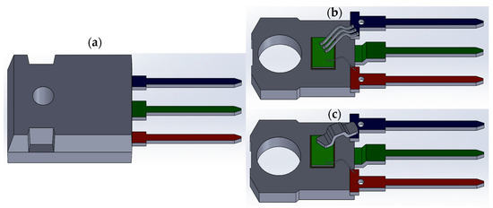
Figure 3.
TO247 MOSFET package models: (a) TO247 MOSFET package with encapsulation; (b) aluminum wire bonded TO247 MOSFET package; (c) copper clip bonded TO247 MOSFET package. The colors indicate key components of the MOSFET package: light green represents the die, deep green represents the drain terminal, blue denotes the source terminal, and red indicates the gate terminal.

Table 1.
Material properties assigned to TO247 MOSFET package models.
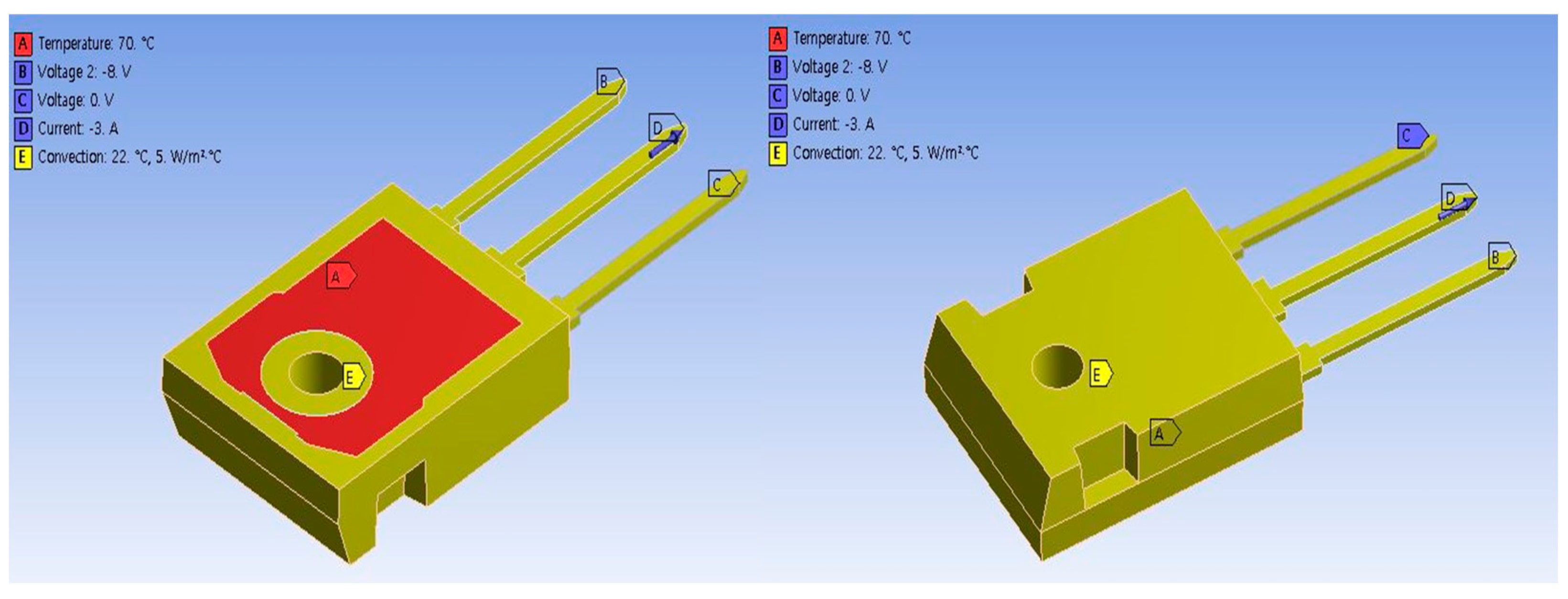
Establishing boundary conditions is crucial to creating a realistic simulation environment that considers the physical operation of the power MOSFET. Figure 4 illustrates the specific locations of the applied boundary conditions. To simulate the electrical behavior and control of the MOSFET, boundary conditions were applied to the source, gate, drain terminals, encapsulation, and surrounding components. Specifically, a potential of 0 V was applied to the source terminal (C), serving as the electrical reference point. The gate terminal (B) was assigned a potential of 8 V to simulate the gate control, while a current of 3 A was directed through the drain terminal (D) to represent the operational current flow. To ensure thermal stability, a constant temperature boundary condition of 70 °C was imposed on the lead frame (A). Additionally, convective boundary conditions were applied to the encapsulation (E) to accurately simulate the thermal interactions with the surrounding components.
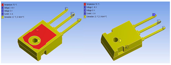
Figure 4.
Applied boundary conditions for the electro−thermal analysis of MOSFET packages; (A) Lead frame, (B) Gate terminal, (C) Source terminal, (D) Drain terminal, (E) Encapsulation.
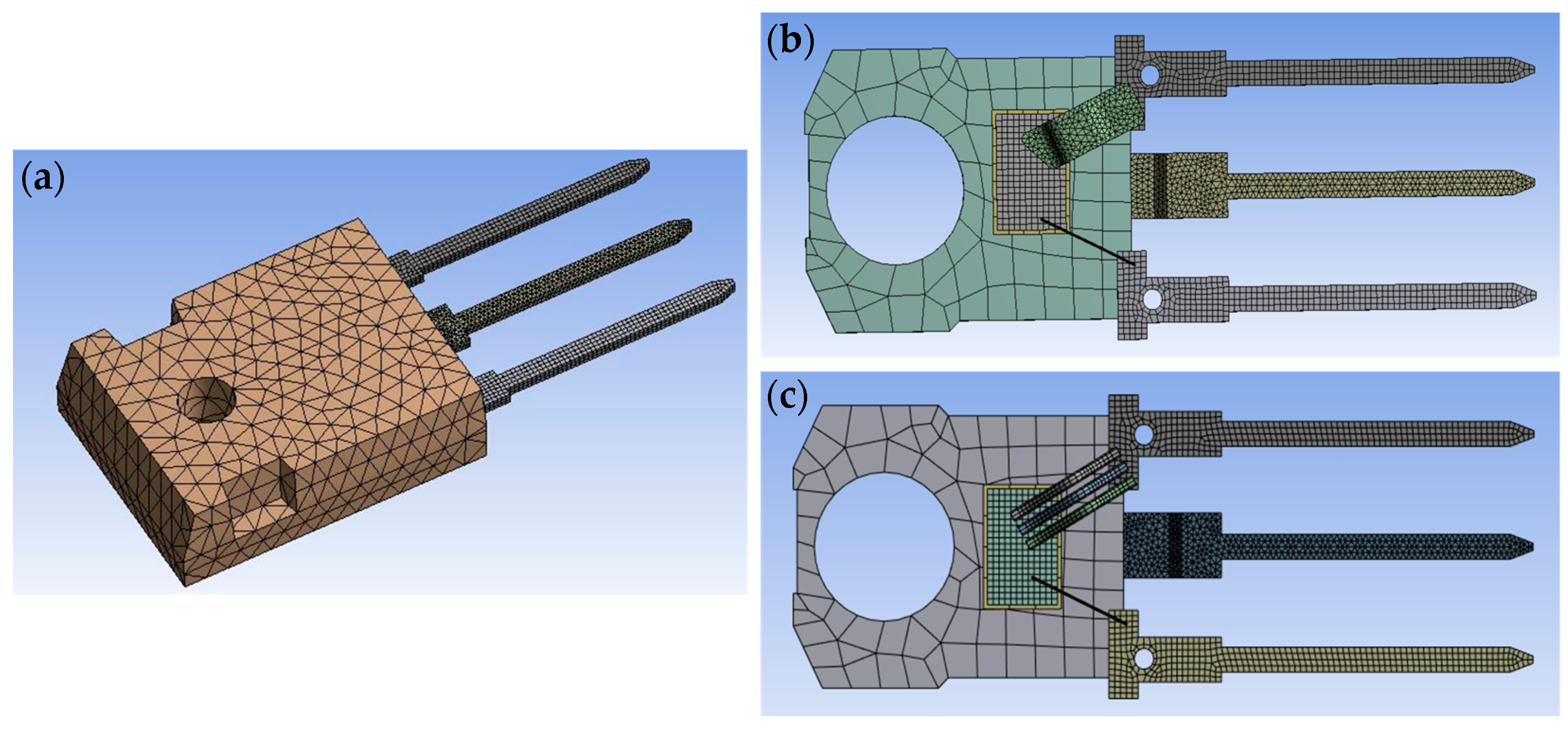
Mesh generation is a crucial step in FEA to ensure numerical stability and computational efficiency, providing the foundation for a detailed representation of the thermal and electrical behavior within a MOSFET. Figure 5 displays the model imported into ANSYS, after the mesh generation process was completed. The mesh was created with careful consideration of the mesh size and distribution to strike a balance between accuracy and computational cost. Fine meshes were used in the areas of interest, namely the die, source, gate, and drain region, while coarser meshes were used in the other areas. The mesh generation resulted in 13,700 elements for the aluminum wire model and 18,554 elements for the copper clip model. For the electro-thermal analysis in ANSYS, the Solid186 element was used, an element frequently employed in 3D thermal conduction analysis that is particularly well-suited for modeling heat transfer within solid materials.

Figure 5.
Mesh generated for TO247 MOSFET package models: (a) mesh generated for TO247 MOSFET package with encapsulation; (b) mesh generated for copper clip bonded TO247 MOSFET package; (c) mesh generated for aluminum wire bonded TO247 MOSFET package.
2.2. DoEs Using LHS
The Design of Experiments (DoEs) is a mathematical technique to establish the connection between variables influencing a process and the process’s output. In this study, the DoEs was employed using Latin Hypercube Sampling (LHS) to generate a comprehensive and diverse set of design points for the copper clip bonding parameters. LHS is a statistical technique used to produce a sample collection of logical parameter values from within a multidimensional distribution [40]. This ensures that the entire range of each parameter is explored by dividing the range into equally probable intervals and sampling each interval exactly once. LHS is particularly effective for FEA simulations, where exploring the parameter space comprehensively and efficiently is essential [41,42]. By ensuring that each parameter is sampled across its entire range, LHS provides a more thorough understanding of the parameter’s impact on the simulation results.
The first step in the DoEs was to identify the key parameters influencing the thermal performance of the copper clips. These key parameters included the horizontal length from the edge of the die to the clip, the clip thickness, and the width. Figure 6 illustrates these parameters, labeled as (a), (b), and (c), respectively, as they were set for the thermal and electrical analysis within a MOSFET. Parameter (a) denotes the horizontal length adjustment from the original length of the die edge to the clip, (b) represents the width of the clip, and (c) signifies the thickness of the clip. By varying parameter (a), the contact area between the clip and the die is altered, which directly impacts the thermal performance. Each parameter was assigned a specific range, based on practical manufacturing constraints and operational requirements. The bounds for these parameters are specified as ranging from: (a) (−0.600 to 0.600) mm, (b) (0.250 to 0.750) mm, and (c) (1.00 to 3.00) mm. LHS was then employed to sample these three parameters, resulting in 250 unique samples within the specified bounds. This involved dividing the range of each parameter into 250 equally probable intervals, followed by the random selection of one value from each interval. This method ensures that each of the 250 samples is unique and covers the entire range of possible values, providing a comprehensive understanding of how these parameters influence the simulation results.
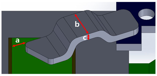
Figure 6.
Parameters defined for the DoEs: (a) horizontal length from the edge to the clip; (b) width of the clip; (c) thickness of the clip.
2.3. Surrogate Model Selection and Validation
SBO is a powerful technique to tackle the computational expense of evaluating high-fidelity simulations for each design iteration. The core idea is to create a surrogate model that approximates the behavior of the actual simulation model, but at significantly reduced computational cost. This surrogate model, trained on the data obtained from FEA simulations, serves as a proxy to predict the thermal performance for new design points, thereby accelerating the optimization process [43,44].
The surrogate model selection methodology involves evaluating multiple models to predict the thermal performance of the MOSFET packages. The following steps outline the process, including data preparation, model definition, evaluation, and visualization of the results. Initially, the dataset obtained from the LHS-based FEA of the MOSFET is divided into training and test subsets using a standard 80:20 split. This division ensures that 80% of the data is used to train the surrogate models, while the remaining 20% is reserved for testing and validation. This approach helps in assessing the model’s ability to generalize to unseen data. To enhance the performance of certain models, particularly those sensitive to input data scales, such as support vector machines and neural networks, the features undergo standardization. The characteristics of the training and test sets are adjusted using standard scaling to ensure that they have a mean of zero and a standard deviation of one. This standardization process is crucial to improve the accuracy and reliability of these models [45,46,47].
A variety of surrogate models are used to evaluate the thermal prediction capability of the models. Firstly, linear regression was applied using the ordinary least squares method to fit a linear relationship between the input parameter values and the target temperature. The model is trained by minimizing the sum of the squared errors between the predicted and actual target values, ensuring the best linear fit to the data. Polynomial regression extends the linear model by applying a second-degree polynomial transformation to the input parameter values. This transformation allows the model to capture non-linear interactions between the parameters before fitting a linear regression model. The training process involves first transforming the input parameters into polynomial terms and then applying the ordinary least squares method to minimize the prediction error. Kriging was also employed due to its ability to model complex, non-linear relationships, while providing uncertainty estimates for the predictions. A Matérn kernel was selected for Kriging, offering flexibility in handling various levels of smoothness in the data. The Kriging surrogate model is further described in detail in Section 2.4. KNN was utilized as a non-parametric regression method, relying on the proximity of the data points. The model is trained by memorizing the entire training dataset and making predictions based on the average values of the nearest neighbors in the parameter space. The number of neighbors was set to 5 and uniform weighting was selected to ensure that all the neighbors contributed equally to the prediction, allowing the model to capture local patterns in the data. No explicit training phase is required beyond storing the training data, but the prediction process involves finding the nearest neighbors for each test point and averaging their target values. SVR, another model included in the evaluation, was applied using the Radial Basis Function (RBF) kernel. This kernel is particularly effective for capturing non-linear dependencies between the input parameters and the target variable, making SVR well-suited for complex data structures. SVR is trained by solving a convex optimization problem that minimizes a regularized hinge loss function. The model learns by finding a hyperplane that separates the data with the maximum margin, while controlling the trade-off between model complexity and prediction error using the regularization parameter. A regularization parameter of 1 is chosen for the current case. Finally, a neural network model was implemented using the Multi-Layer Perceptron (MLP) architecture. The neural network consists of a single hidden layer with 100 neurons, utilizing the Rectified Linear Unit (ReLU) activation function to facilitate faster convergence and overcome the vanishing gradient problem. The Adam optimizer was used for training, which dynamically adjusts the learning rate during training. The network was trained on 5000 iterations, with an initial learning rate of 0.01. The training process involved backpropagation, where the model’s weights were updated iteratively based on the error between the predicted and actual target values, ensuring that the model could effectively learn complex relationships involving the parameters, while avoiding overfitting.
To evaluate the performance of each surrogate model, predictions are compared against the actual values from the test set. The models are assessed using metrics such as the mean squared error (MSE), R-squared (R2), and adjusted R-squared (adjusted R2). These metrics offer information about the precision of the models and their capacity for explanation. The average squared difference between the actual and anticipated values is measured by the MSE. The ratio of predicted variance in the target variable derived from the input features is denoted by R2. A higher value indicates a better fit. For multiple regression scenarios, the adjusted R2 offers a more precise way to quantify the performance of the model by adjusting the R2 value according to the number of predictors in the model. The equations for the MSE, R2, and adjusted R2 are as follows [48]:
where represents the true value, is the predicted value, is the mean of the actual values, is the total number of data points, and is the number of predictors in the model.
2.4. Kriging-Based Genetic Algorithm
Kriging, Gaussian process regression (GPR), a non-parametric, Bayesian regression technique, offers a robust and adaptable structure to simulate intricate datasets. It defines a priori over functions and updates this prior with observed data to form a posterior distribution over functions.
In Kriging, the response value from a simulation at any given point is estimated using a combination of a known polynomial and a random deviation from that polynomial. The equation for Kriging is written as:
where represents the unknown response of interest, is a specified polynomial, and is regarded as a realization of a random Gaussian process with a mean of zero, a variance of , and a non-zero covariance, commonly referred to as a kernel [49]. The term offers a broad approximation of the design space, while adds a localized deviation, allowing the Kriging model to accurately incorporate the observed data points. The dispersion matrix of is given by:
where R is an square matrix that is symmetrical, where each diagonal element is filled with ones, is the number of observed points, and is the correlation function between any two observed points and that corresponds to the off-diagonal elements in the matrix. In this study, the Matérn kernel is employed to define the covariance between any two points and , and defined by [50,51]:
where controls the smoothness of the function, is the length scale between the points, is the gamma function, and is the modified Bessel function of the second kind. Here, and are chosen to be (2.5 and 1), respectively, to achieve a smooth function and moderate collation between the points. The prediction at a new point is computed as [52]:
where y is the column vector of length containing the values of the response at each observed point and is a column vector with components, which when is constant are ones. The and in Equation (7) are given by:
The estimate of variance for the Kriging model is calculated using:
To train the Kriging model, 250 simulation results on the maximum temperature obtained through LHS and FEA are utilized. The trained Kriging model utilizes this data to construct a predictive surrogate model, which is then used to estimate the maximum temperature at any given point within the parameter space. The trained Kriging model is subsequently employed as the objective function in a GA to facilitate the optimization.
A GA is an optimization method inspired by the principles of natural selection and genetics. It is used to iteratively apply procedures like selection, crossover, and mutation, to find approximations for solutions to complex problems. A GA evaluates predicted values by comparing them to target outputs using an objective function, which serves as a fitness measure to guide the optimization [53]. The optimization of the MOSFET copper clip involves multiple constraints and non-linear relationships, as it addresses complex interactions between the dimensions of the copper clip and the thermal performance requirements. The GA is well-suited to such complex and constrained optimization tasks because of its inherent flexibility and ability to handle non-convex and non-linear optimization landscapes. Unlike other algorithms, such as Particle Swarm Optimization (PSO) and Differential Evolution (DE), the GA maintains a population of potential solutions, which helps explore a broader solution space and avoid being trapped in local optima risk that can be higher with simpler algorithms like PSO, particularly in regard to multi-modal problems [54].
In this study, the tournament selection function is used at the selection stage for the GA, where three parameters are arbitrarily chosen from the population, and the one with the highest fitness score is chosen, ensuring that higher fitness individuals are more likely to propagate their genetic material [55]. The crossover function employs a single-point crossover method [56], where two parent individuals recombine with a crossover rate of 0.9 to produce two new offspring. If a randomly generated number is less than the crossover rate, a crossover point is selected, and the parents exchange genetic material at this point, promoting genetic diversity. The mutation function uses bit-flip mutation, where each bit in an offspring’s binary string is flipped with a probability equal to the mutation rate, which is dynamically calculated based on the number of bits and variables [57]. Mutation introduces random changes to maintain diversity within the population and prevent premature convergence.
The population size is set at 100 individuals, ensuring that sufficient potential solutions are evaluated in each generation, balancing diversity and computational efficiency. Each individual is encoded with 16 bits per variable, providing a precise representation and a granular search space. The optimization process iteratively evaluates new offspring for each generation, continuing until it either reaches predefined precision criteria, or completes the maximum number of generations set. These parameters and methods are chosen to balance exploration and exploitation, ensuring a diverse and evolving population that converges toward optimal solutions over generations. By iteratively applying selection to choose the best individuals based on their fitness, crossover to combine genetic material, and mutation to introduce diversity, the GA improves the population’s overall fitness and converges toward an optimal solution. While real-coded GAs are known for offering higher precision during continuous variable optimization [58], the results presented later in Section 3.4 show that the binary-coded GA used in this study provides results that are both accurate and effective. Under various temperature restrictions, the predicted temperatures from the Kriging–GA model closely match the simulated temperatures, with percentage errors of 2.66% for no restriction, 0.403% for the 75 °C restriction, and 0.251% for the 80 °C restriction, as discussed later in Section 3.4. The minor differences between the predicted and simulated temperatures indicate that, despite the inherent limitations of binary coding, the method delivers sufficient accuracy for practical engineering applications.
GA optimization is employed to optimize the input parameters to ensure that the maximum temperature is minimized, while adhering to specific temperature constraints. The optimization process is run under three different scenarios: without any temperature restriction, with a minimum temperature restriction of 75 °C, and with a minimum temperature restriction of 80 °C. The constraints in the optimization problem, including the parameter bounds and temperature restrictions, are managed through two key mechanisms. First, the parameter bounds are enforced by encoding the design variables as binary strings, which are then decoded into real values within the specified limits, (a) (−0.600 to 0.600) mm, (b) (0.250 to 0.750) mm, and (c) (1.00 to 3.00) mm. This ensures that the GA only explores solutions within the valid parameter ranges. Second, the temperature restrictions are handled through a penalty function within the objective function. A threshold temperature is defined for 75 °C and 80 °C, and if the predicted temperature from the model falls below this threshold, a penalty is applied, proportional to the square of the difference between the threshold and the predicted result. This penalty ensures that solutions that do not meet the temperature requirement are penalized, guiding the GA toward feasible solutions that satisfy both the parameter bounds and the temperature constraints.
During the implementation of this GA, the convergence of the optimization process is controlled by two key criteria, the fitness precision and the maximum number of generations. The fitness precision criterion monitors the improvement in terms of the best solution between successive generations. If the difference in the fitness value falls below a predefined threshold, set to 1 × 10⁻⁵ in this case, the algorithm considers the solution sufficiently optimized and begins the process of termination. On the other hand, the maximum number of generations serves as a secondary safeguard, ensuring that the algorithm does not run indefinitely. This is set to 30, meaning that the algorithm will terminate after 30 iterations if it has not already met the fitness precision requirement. This entire optimization process, including parameter encoding, penalty handling, and optimization under various temperature constraints, is implemented and executed using Python 3.10.9.
PSO and DE are employed alongside the GA to evaluate and compare their performance in optimizing the given objective function. Both PSO and DE are configured to have the same population size and maximum number of iterations as the GA to ensure a consistent and fair comparison across all the algorithms in terms of computational resources and population dynamics. PSO is a swarm-based optimization algorithm that simulates the social behavior of particles exploring the solution space [59]. In this study, the swarm size is set equal to the GA’s population size, allowing each particle to adjust its position based on both its personal best solution and the global best solution discovered by the swarm. The search space is constrained by the parameter bounds described in Section 2.2 for the design variables, ensuring that all the particles explore the space within the predefined parameter boundaries. DE, on the other hand, evolves a population of candidate solutions through a process of mutation and recombination [60]. The mutation factor is set between 0.5 and 1 to balance exploration and exploitation, while the recombination rate is fixed at 0.7, meaning that 70% of the parameters in the new solution are derived from the base vector. Additionally, DE utilizes a strategy that focuses on using the best solution in the current population as the base for generating new candidate solutions. This strategy ensures that the algorithm continuously builds on the best-known solutions during the optimization process. Both PSO and DE are designed to run for the same number of iterations as the GA, enabling a controlled experimental setup that focuses on evaluating each algorithm’s optimization effectiveness.
3. Results and Discussion
3.1. Comparison between Al Wire and Cu Clip Bonding Results
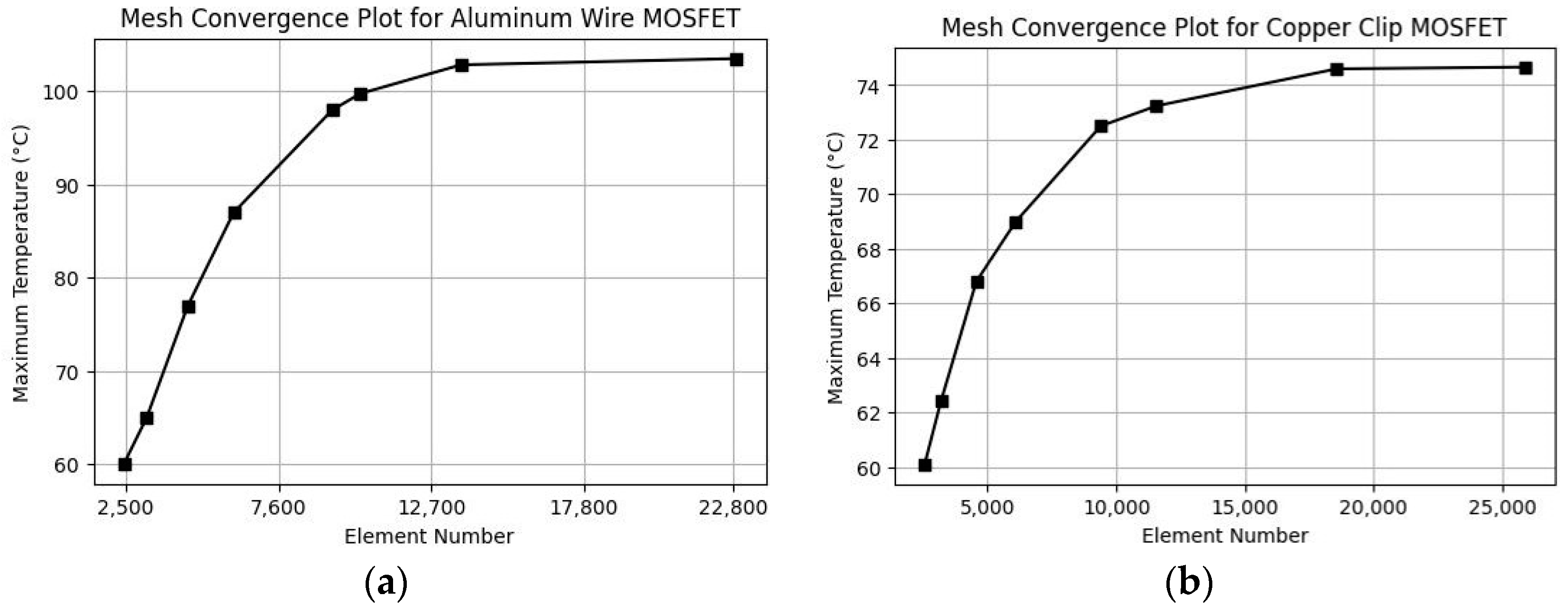
The mesh convergence analysis for both the aluminum wire and copper clip bonding MOSFET packages is shown in Figure 7. For the Al wire bonded MOSFET package, the number of elements ranged from 2435 to 22,876. The maximum temperature increased from 60.1 °C at 2435 elements to 103.5 °C at 22,876 elements. Convergence occurred around 13,700 elements, where the temperature stabilized at 102.8 °C. Just before convergence, at 10,340 elements, the temperature was 99.8 °C. The percentage difference between the temperature in the case of 10,340 elements is approximately 2.96%. At the final element count of 22,876, the temperature increased slightly to 103.5 °C, with a percentage difference of 0.68% compared to the 13,700-element case, indicating that further mesh refinement provided only minimal accuracy improvement. This demonstrates that 13,700 elements are sufficient for this package to achieve accurate results. The copper clip MOSFET package, with element counts ranging from 2557 to 25,945, showed different thermal behavior. The maximum temperature increased from 60.1 °C at 2557 elements to 74.7 °C at 25,876 elements. Convergence was observed at 18,554 elements, where the temperature stabilized at 74.6 °C. Just before convergence, at 11,567 elements, the temperature was 73.2 °C, resulting in a percentage difference of approximately 1.89%. The temperature at the final element count of 25,876 increased slightly to 74.7 °C, with a negligible percentage difference of 0.13%, confirming convergence. In both the aluminum wire and copper clip MOSFET packages, the mesh refinement process began with the critical regions of the device, as shown in Figure 5. As the number of elements increased, other less critical regions were also refined in greater detail to more accurately capture the overall thermal behavior and ensure convergence.
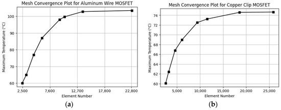
Figure 7.
Mesh convergence plots for MOSFET thermal analysis: (a) mesh convergence for aluminum wire MOSFET; (b) mesh convergence for copper clip MOSFET.
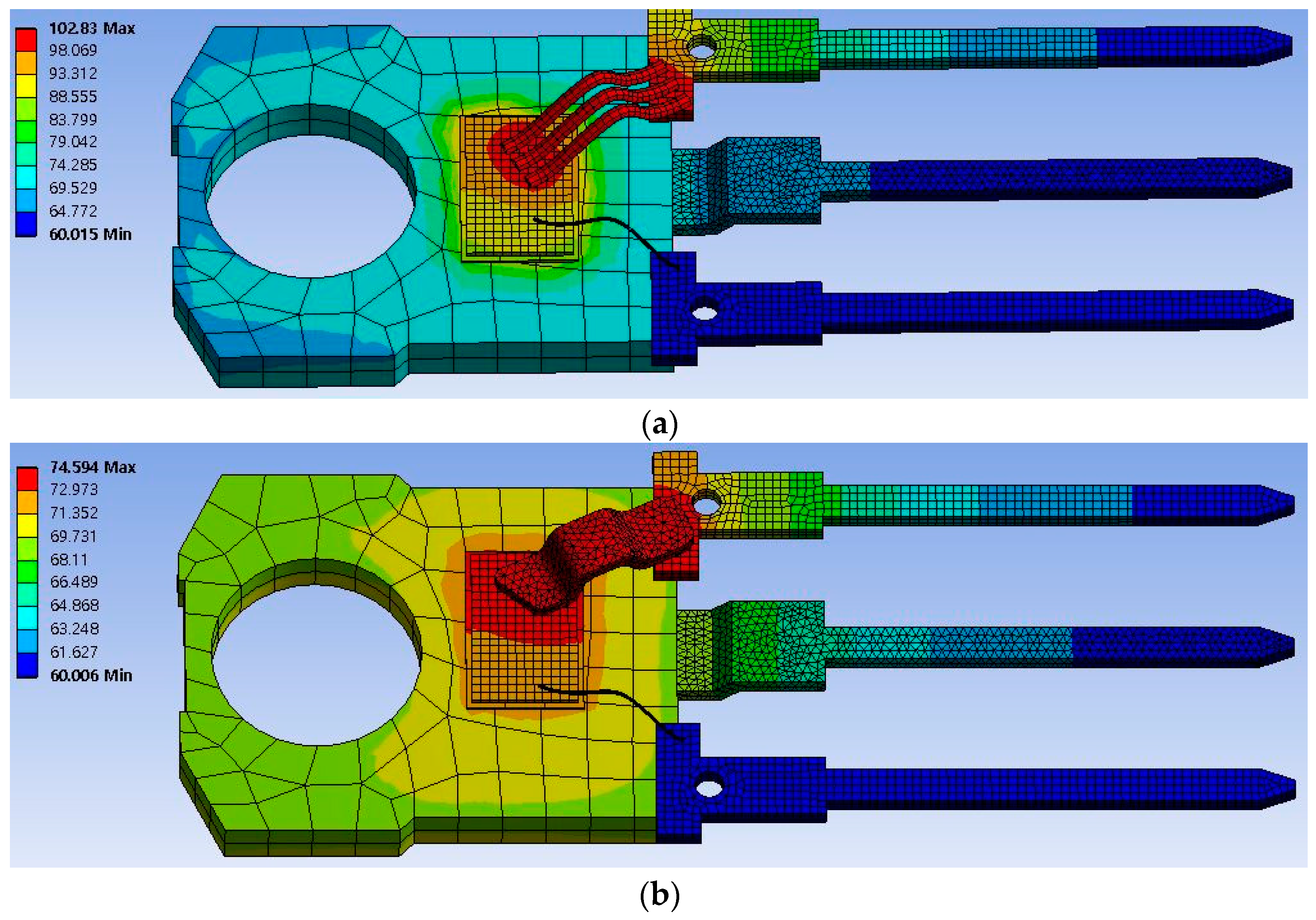
Figure 8 compares aluminum wire and copper clip bonding. The thermal analysis results demonstrate a significant difference in the maximum temperature observed for the two bonding methods. Figure 8a shows the thermal distribution for the aluminum wire bonding configuration. In this scenario, the maximum temperature reached is 102.8 °C, indicating a higher thermal resistance and less efficient heat dissipation. The elevated temperatures are concentrated around the bonding area, suggesting that the aluminum wire’s lower thermal conductivity contributes to the elevated temperatures in the critical regions. Figure 8b depicts the thermal distribution for the copper clip bonding configuration. Here, the maximum temperature is significantly lower at 74.6 °C. The superior thermal conductivity of the copper clip enables more effective heat dissipation, resulting in a more uniform temperature distribution across the MOSFET package and a lower overall maximum temperature. The copper clip bonding method reduces the maximum temperature by approximately 27.5%, compared to the Al wire bonding method, demonstrating a clear advantage in terms of thermal management. This reduction in temperature enhances the reliability of the MOSFET by mitigating thermal stress, while also underscoring the effectiveness of copper clip bonding in promoting efficient thermal management within power electronic modules.
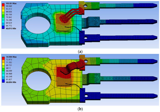
Figure 8.
Thermal analysis results showing temperature distribution: (a) Al wire bonding and (b) copper clip bonding configurations.
3.2. Latin Hypercube Sampling and Simulation Results
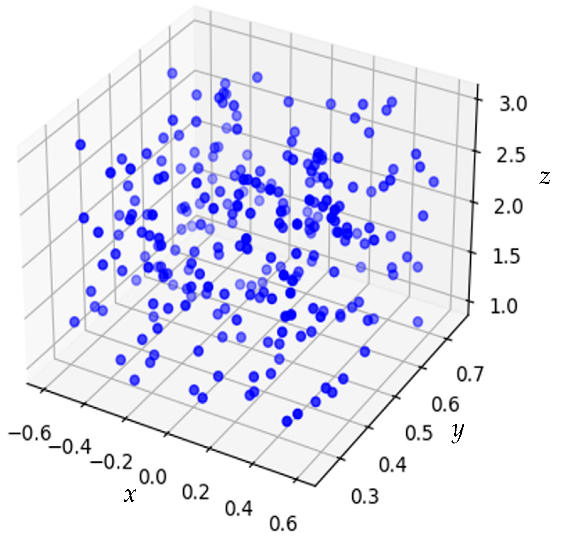
Figure 9 illustrates the 3D scatter plot of the LHS results for the copper clip parameters. In this plot, the x-axis represents parameter (a), the y-axis represents parameter (c), and the z-axis represents parameter (b). The LHS method effectively generated a diverse and well-distributed set of 250 sample points, covering the entire parameter space. This comprehensive sampling ensured that the simulations could capture the variability and interactions between the parameters. Table 2 and Table 3 summarize the statistics of the simulation results, including the mean, standard deviation (Std), minimum value (Min), first quartile (25%), median (50%), third quartile (75%), and maximum value (Max) for the LHS-generated points. For parameter (a), the mean is −0.002 mm, with a standard deviation of 0.349 mm, ranging from (−0.598 to 0.597) mm. Parameter (b) has a mean of 0.501 mm, with a standard deviation of 0.145 mm, and ranges from (0.252 to 0.750) mm. Parameter (c) shows a mean of 2.00 mm, with a standard deviation of 0.577 mm, ranging from (1.00 to 2.99) mm. Finally, in terms of the response, the maximum temperature has a mean of 75.5 °C, with a standard deviation of 3.55 °C, ranging from (60.0 to 91.7) °C.
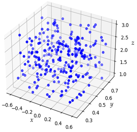
Figure 9.
A 3D scatter plot of the LHS results for the copper clip parameters, where the x-axis represents the parameters. The x-axis, y-axis and z-axis represents the values of parameter a (horizontal length from the die edge to the clip), parameter c (clip thickness), parameter b (clip width), respectively.
Table 2.
Statistical summary of parameters (a, b, c) based on the LHS-based simulation results.
Table 3.
Statistical summary of the maximum temperature based on the LHS-based simulation results.
3.3. Surrogate Model Selection Results
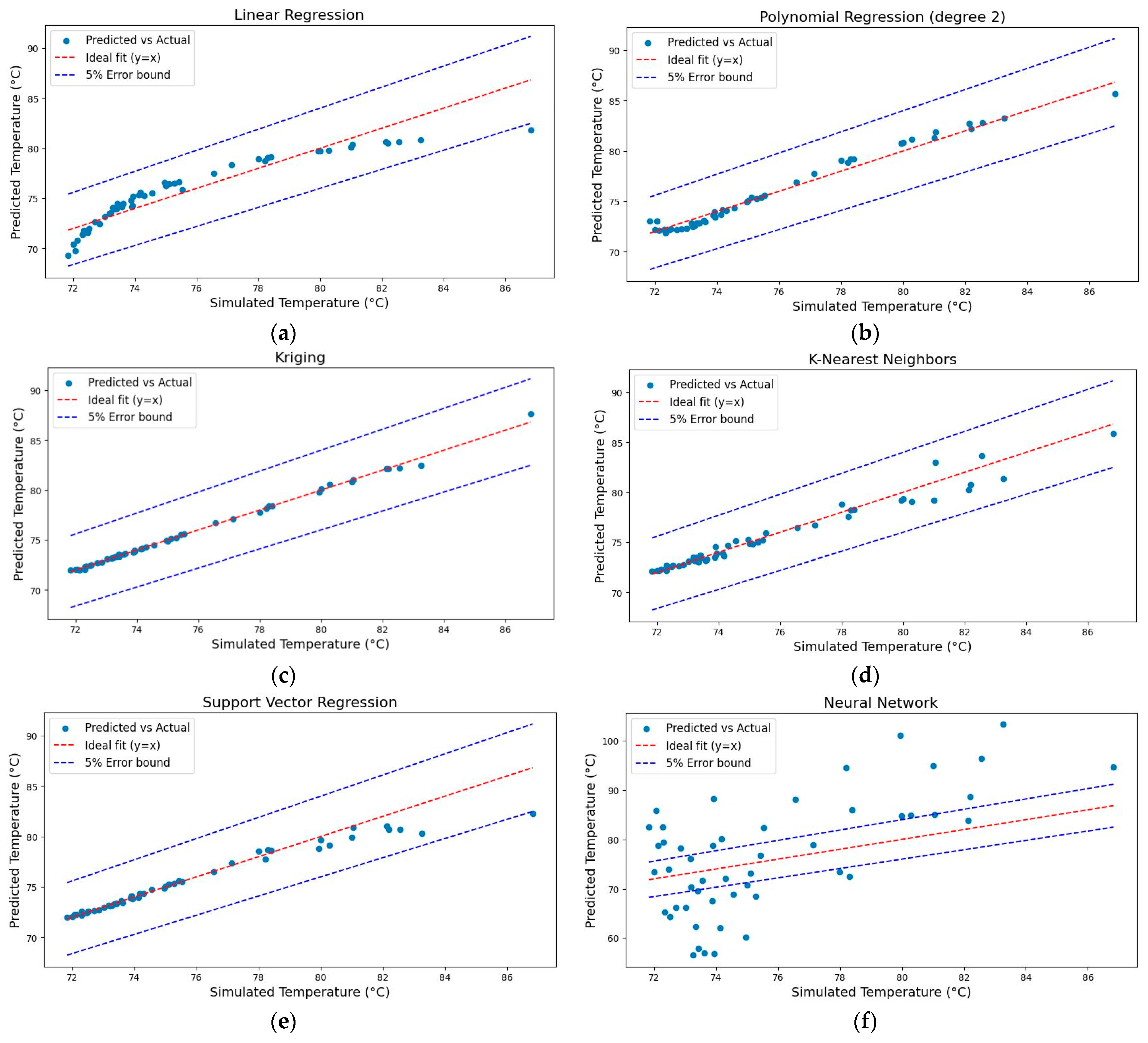
Figure 10 and Table 4 present the results of the surrogate model selection process. Figure 10 presents a series of scatter plots comparing the predicted versus actual temperatures for each surrogate model, including linear regression, polynomial regression (degree 2), Kriging, K-Nearest Neighbors, support vector regression, and the neural network. Each scatter plot features an ideal fit line, where the predicted values equal the actual values, along with a 5% error bound to visually demonstrate the accuracy and reliability of each model. Table 4 provides quantitative metrics for each model, including the MSE, R2, and adjusted R2. These metrics offer rigorous statistical validation of the predictive capabilities of the models, confirming the visual observations from the scatter plots. The combined analysis of these visual and quantitative results allows a clear comparison of the surrogate models, highlighting the most accurate and reliable model to predict the thermal performance of the MOSFETs. In particular, the Kriging model demonstrates superior performance, with lower MSE and higher R2 values, making it the preferred choice for further optimization.
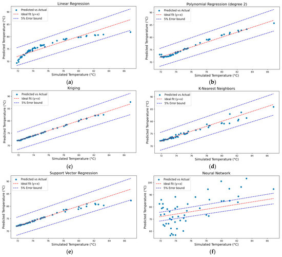
Figure 10.
Comparison of the predicted versus the simulated temperatures for various surrogate models: (a) linear regression; (b) polynomial regression; (c) Kriging regression; (d) RBF regression; (e) support vector regression; (f) neural network.
Table 4.
Performance metrics of various surrogate models chosen for validation.
The evaluation began with simple models like linear regression, which showed limitations in regard to capturing the complex non-linearities present in the data, despite its simplicity and interpretability. With an MSE of 1.72, an R2 value of 0.868, and an adjusted R2 of 0.860, the linear regression model exhibited a moderate fit. The adjusted R2, which accounts for the number of predictors in the model, was slightly adjusted downward, reflecting that the model’s simplicity might not be sufficient to capture the complexity of the data, especially when considering model complexity versus fit. In contrast, the polynomial regression, specifically with a second-degree polynomial, significantly improved the accuracy of the predictions. This model achieved an MSE of 0.305, an R2 value of 0.977, and an adjusted R2 of 0.970. The high adjusted R2 indicates that the additional complexity introduced by the polynomial terms was justified, as it resulted in a better fit to the data, without overfitting. However, the Kriging regression model emerged as the most accurate and reliable model in this study. It delivered the lowest MSE of 0.036, the highest R2 value of 0.997, and an equally impressive adjusted R2 of 0.997. These results validate the selection of the Kriging model, affirming its robustness in capturing complex data patterns and making it the optimal choice for the surrogate model in this context. The high adjusted R2 suggests that this model fits the data exceptionally well, while also doing so with a complexity that is appropriate for the given dataset.
Other models, such as the K-Nearest Neighbors and SVR, demonstrated reasonable performance, with adjusted R2 values of (0.959 and 0.933), respectively, but they did not match the accuracy of the Kriging surrogate model. These models also showed that their complexity was well-suited to the data, though in terms of predictive accuracy, they still fell short of the Gaussian process. Notably, the neural network model performed poorly, with an exceptionally high MSE of 90.3, a negative R2 value of −5.91, and an adjusted R2 of −6.36. The negative adjusted R2 further emphasizes the model’s inadequacy, as it indicates that the neural network’s complexity was not only unjustified, but also detrimental to its predictive performance. This poor performance can be attributed to several factors. Neural networks, while powerful, require careful tuning of the hyperparameters, such as the learning rate, number of layers, and number of neurons per layer. If these parameters are not optimally configured, the model can easily overfit or underfit the data. In this case, the neural network likely overfitted the training data, failing to generalize to the test data, as indicated by the negative R2 and adjusted R2 values. Additionally, the small dataset size relative to the complexity of the neural network might have contributed to its inability to learn meaningful patterns, leading to poor predictive performance. This result underscores the importance of model selection and tuning, particularly when using complex models like neural networks, which require substantial data and careful configuration to perform well.
3.4. Kriging–GA-Based Optimization Results
A comparison between the GA, PSO, and DE in terms of the parameter and temperature estimation is given in Table 5. Each algorithm is run 30 times and the mean and standard deviation values of the estimated parameters are calculated. The GA demonstrates the lowest standard deviation in regard to both the estimated parameter values (a, b, c) and the maximum temperature achieved. Specifically, the GA produced mean parameter values of (a = 0.597, b = 0.750, c = 2.994), with a minimal standard deviation of (1.64 × 10⁻⁴, 1.15 × 10⁻⁴, 9.57 × 10⁻⁵). Additionally, the mean maximum temperature obtained using the GA was 69.6 °C, with a low standard deviation of 0.105 °C, reflecting its ability to converge similar solutions across multiple trials. In contrast, PSO, while achieving a mean parameter value of (a = −0.120, b = 0.551, c = 2.995) and a slightly lower mean temperature of 69.3 °C, exhibited higher variability, with a standard deviation of 0.255 °C and parameter deviations of (5.86 × 10⁻¹, 2.44 × 10⁻¹, 4.44 × 10⁻¹⁶). This suggests that PSO, though capable of producing good results, is less consistent across the runs. DE achieved mean parameter values of (a = 0.278, b = 0.684, c = 2.995) and a mean temperature of 69.5 °C, but with higher variability than the GA, as indicated by a standard deviation of 0.336 °C for the temperature and (5.29 × 10⁻¹, 1.69 × 10⁻¹, 3.42 × 10⁻¹⁶) for the parameters.
Table 5.
Comparison of GA, PSO, and DE in terms of parameter and temperature estimation.
PSO may occasionally outperform the GA in terms of temperature minimization; the GA offers the most consistent and reliable performance, making it the most suitable algorithm for applications where precision and repeatability are paramount. DE serves as the middle ground between the GA and PSO, with reasonable consistency and competitive results, but still displaying more variability than the GA. Additionally, the parameter values obtained from the GA are closely aligned with those that yield the lowest maximum temperature, further supporting the choice of the GA as the preferred optimization algorithm in this study.
Table 6 provides a comprehensive overview of the optimized parameters across different temperature restriction scenarios, illustrating how the Kriging-based GA optimization model adjusts these values to meet specific constraints. In the scenario without any restrictions, the parameters resulted in a predicted temperature of 69.6 °C and simulated temperatures of 71.5 °C, demonstrating a percentage error of 2.66%. Under the 75.0 °C restriction, the parameters led to a predicted temperature of 74.8 °C, which closely matched the simulated temperature of 74.5 °C, resulting in a minor error of 0.403%. Similarly, with the 80.0 °C restriction, the model produced parameters yielding a predicted temperature of 79.8 °C and a simulated temperature of 79.6 °C, with an even smaller error of 0.251%. Across all scenarios, the percentage errors were minimal, underscoring the accuracy and reliability of the model in predicting temperatures, despite varying constraints. The optimized parameters highlight the ability of the Kriging–GA model to effectively navigate these constraints, ensuring the best possible outcomes, while maintaining precise temperature control. This precision is particularly important in applications where maintaining specific temperature thresholds is critical for operational stability and performance.
Table 6.
Optimized parameters and temperature predictions under various temperature restrictions using the Kriging–GA model.
4. Conclusions
This study conducted FEA of the electro-thermal behavior of a MOSFET with copper clip bonding, employing LHS for robust parameter exploration. The analysis demonstrated that the aluminum wire bonding model exhibited a maximum temperature of 102.8 °C, which was significantly higher, compared to the peak temperature of the original copper clip bonding model of 74.6 °C. To enhance the predictive capabilities regarding the electro-thermal behavior, a surrogate model selection process was performed. Among the various models evaluated, including linear regression, polynomial regression, and neural networks, the Kriging regression model demonstrated superior performance. Specifically, the Kriging model achieved a low MSE of 0.036, along with a high R2 of 0.997, and an adjusted R2 of 0.997. These metrics confirmed the superior accuracy of the model and its ability to replicate complex system behaviors with reduced computational resources, making it the optimal choice for subsequent optimization tasks.
Following the selection of the Kriging model, the study proceeded to optimize the thermal performance of the MOSFET under different temperature constraints. Through the application of the Kriging–GA-based optimization, the optimized copper clip design achieved a further reduction in the maximum temperature to 71.5 °C, representing a 4.20% improvement over the original copper clip model, and a substantial 43.8% reduction compared to the aluminum wire bonding model. The adoption of the Kriging–GA model both enhanced the thermal management of the MOSFET and significantly reduced the computational power required for the optimization process. The efficiency of the model in approximating the FEA results enabled extensive parameter space exploration with minimal computational demand, providing a critical advantage in regard to complex electro-thermal analyses. These findings emphasize the dual benefits of the Kriging model in terms of high accuracy and computational efficiency, offering a robust tool for optimizing power electronic systems under stringent thermal constraints. Future work should focus on the experimental validation of the optimized designs to confirm the simulation results and address any practical challenges that may arise during real-world applications. Additionally, exploring the integration of the Kriging model with more advanced or hybrid optimization techniques could further enhance its effectiveness in regard to complex engineering problems.
Author Contributions
Conceptualization, Y.C. and S.K.; methodology, Y.C.; software, Y.C., J.J. and D.K.; writing—original draft preparation, Y.C.; writing—review and editing, S.K. and H.S.K.; supervision, H.S.K.; project administration, H.S.K.; funding acquisition, H.S.K. All authors have read and agreed to the published version of the manuscript.
Funding
This work was supported by the National Research Foundation of Korea (NRF), grant funded by the Korean government (MSIT) (RS-2024-00405691).
Data Availability Statement
The original contributions presented in the study are included in the article, further inquiries can be directed to the corresponding author/s.
Conflicts of Interest
The authors declare that there are no conflicts of interest.
Nomenclature
| Acronym | Definition |
| CAD | Computer-Aided Design modeling |
| DoEs | Design of Experiments |
| FEA | Finite Element Analysis |
| FEM | Finite Element Method |
| GA | Genetic Algorithm |
| GPR | Gaussian Process Regression |
| LHS | Latin Hypercube Sampling |
| MSE | Mean Squared Error |
| MOSFETs | Metal–Oxide–Semiconductor Field-Effect Transistors |
| RBF | Radial Basis Function |
| R2 | R-squared |
References
- Marzoughi, A.; Burgos, R.; Boroyevich, D. Investigating Impact of Emerging Medium-Voltage SiC MOSFETs on Medium-Voltage High-Power Industrial Motor Drives. IEEE J. Emerg. Sel. Top. Power Electron. 2019, 7, 1371–1387. [Google Scholar] [CrossRef]
- Gao, R.; Yang, L.; Yu, W.; Husain, I. Gate Driver Design for a High Power Density EV/HEV Traction Drive Using Silicon Carbide MOSFET Six-Pack Power Modules. In Proceedings of the 2017 IEEE Energy Conversion Congress and Exposition (ECCE), Cincinnati, OH, USA, 7 October 2017; pp. 2546–2551. [Google Scholar]
- Tasca, D.M. Pulse Power Failure Modes in Semiconductors. IEEE Trans. Nucl. Sci. 1970, 17, 364–372. [Google Scholar] [CrossRef]
- Hou, F.; Wang, W.; Cao, L.; Li, J.; Su, M.; Lin, T.; Zhang, G.; Ferreira, B. Review of Packaging Schemes for Power Module. IEEE J. Emerg. Sel. Top. Power Electron. 2020, 8, 223–238. [Google Scholar] [CrossRef]
- Liu, C.; Liu, A.; Jiang, H.; Liang, S.; Zhou, Z.; Liu, C. Self-Propagating Exothermic Reaction Assisted Cu Clip Bonding for Effective High-Power Electronics Packaging. Microelectron. Reliab. 2022, 138, 114688. [Google Scholar] [CrossRef]
- Yasui, K.; Morikawa, T.; Hayakawa, S.; Funaki, T. Performance Improvement for 3.3 kV 1000 A High Power Density Full-SiC Power Modules with Sintered Copper Die Attach. IEEE J. Emerg. Sel. Top. Power Electron. 2024, 1. [Google Scholar] [CrossRef]
- Wang, L.; Zhang, T.; Yang, F.; Ma, D.; Zhao, C.; Pei, Y.; Gan, Y. Cu Clip-Bonding Method With Optimized Source Inductance for Current Balancing in Multichip SiC MOSFET Power Module. IEEE Trans. Power Electron. 2022, 37, 7952–7964. [Google Scholar] [CrossRef]
- Herbsommer, J.A.; Noquil, J.; Bull, C.; Lopez, O. Novel Thermally Enhanced Power Package. In Proceedings of the 2010 Twenty-Fifth Annual IEEE Applied Power Electronics Conference and Exposition (APEC), Palm Springs, CA, USA, 21–25 February 2010; pp. 398–400. [Google Scholar]
- Zhu, Q.; Forsyth, A.; Todd, R.; Mills, L. Thermal Characterisation of a Copper-Clip-Bonded IGBT Module with Double-Sided Cooling. In Proceedings of the 2017 23rd International Workshop on Thermal Investigations of ICs and Systems (THERMINIC), Amsterdam, The Netherlands, 27–29 September 2017; pp. 1–6. [Google Scholar]
- Kim, D.-H.; Oh, A.-S.; Park, E.-Y.; Kim, K.-H.; Jeon, S.-J.; Bae, H.-C. Thermal and Electrical Reliability Analysis of TO-247 for Bonding Method, Substrate Structure and Heat Dissipation Bonding Material. In Proceedings of the 2021 IEEE 71st Electronic Components and Technology Conference (ECTC), San Diego, CA, USA, 1 June 2021; pp. 1950–1956. [Google Scholar]
- Liu, B.; Koziel, S.; Zhang, Q. A Multi-Fidelity Surrogate-Model-Assisted Evolutionary Algorithm for Computationally Expensive Optimization Problems. J. Comput. Sci. 2016, 12, 28–37. [Google Scholar] [CrossRef]
- Cai, X.; Gao, L.; Li, X. Efficient Generalized Surrogate-Assisted Evolutionary Algorithm for High-Dimensional Expensive Problems. IEEE Trans. Evol. Comput. 2020, 24, 365–379. [Google Scholar] [CrossRef]
- Karlsson, R.; Bliek, L.; Verwer, S.; de Weerdt, M. Continuous Surrogate-Based Optimization Algorithms Are Well-Suited for Expensive Discrete Problems. In Proceedings of the Artificial Intelligence and Machine Learning; Baratchi, M., Cao, L., Kosters, W.A., Lijffijt, J., van Rijn, J.N., Takes, F.W., Eds.; Springer International Publishing: Cham, Switzerland, 2021; pp. 48–63. [Google Scholar]
- Fraehr, N.; Wang, Q.J.; Wu, W.; Nathan, R. Assessment of Surrogate Models for Flood Inundation: The Physics-Guided LSG Model vs. State-of-the-Art Machine Learning Models. Water Res. 2024, 252, 121202. [Google Scholar] [CrossRef]
- Cozad, A.; Sahinidis, N.V.; Miller, D.C. Learning Surrogate Models for Simulation-Based Optimization. AIChE J. 2014, 60, 2211–2227. [Google Scholar] [CrossRef]
- Alizadeh, R.; Allen, J.K.; Mistree, F. Managing Computational Complexity Using Surrogate Models: A Critical Review. Res. Eng. Des. 2020, 31, 275–298. [Google Scholar] [CrossRef]
- Bhosekar, A.; Ierapetritou, M. Advances in Surrogate Based Modeling, Feasibility Analysis, and Optimization: A Review. Comput. Chem. Eng. 2018, 108, 250–267. [Google Scholar] [CrossRef]
- Tyan, M.; Nguyen, N.V.; Lee, J.-W. A Tailless UAV Multidisciplinary Design Optimization Using Global Variable Fidelity Modeling. IJASS 2017, 18, 662–674. [Google Scholar] [CrossRef]
- Tian, K.; Gao, T.; Hu, X.; Xiao, J.; Liu, Y. Novel Optimal Sensor Placement Method towards the High-Precision Digital Twin for Complex Curved Structures. Int. J. Solids Struct. 2024, 302, 113003. [Google Scholar] [CrossRef]
- Cheng, K.; Lu, Z.; Ling, C.; Zhou, S. Surrogate-Assisted Global Sensitivity Analysis: An Overview. Struct. Multidiscip. Optim. 2020, 61, 1187–1213. [Google Scholar] [CrossRef]
- McBride, K.; Sundmacher, K. Overview of Surrogate Modeling in Chemical Process Engineering. Chem. Ing. Tech. 2019, 91, 228–239. [Google Scholar] [CrossRef]
- Hong, X.; Mitchell, R.J.; Chen, S.; Harris, C.J.; Li, K.; Irwin, G.W. Model Selection Approaches for Non-Linear System Identification: A Review. Int. J. Syst. Sci. 2008, 39, 925–946. [Google Scholar] [CrossRef]
- Wang, P.; Lu, Z.; Tang, Z. An Application of the Kriging Method in Global Sensitivity Analysis with Parameter Uncertainty. Appl. Math. Model. 2013, 37, 6543–6555. [Google Scholar] [CrossRef]
- Takoutsing, B.; Heuvelink, G.B.M. Comparing the Prediction Performance, Uncertainty Quantification and Extrapolation Potential of Regression Kriging and Random Forest While Accounting for Soil Measurement Errors. Geoderma 2022, 428, 116192. [Google Scholar] [CrossRef]
- Palar, P.S.; Shimoyama, K. On Efficient Global Optimization via Universal Kriging Surrogate Models. Struct. Multidiscip. Optim. 2018, 57, 2377–2397. Available online: https://link.springer.com/article/10.1007/s00158-017-1867-1 (accessed on 2 August 2024). [CrossRef]
- Moustapha, M.; Sudret, B.; Bourinet, J.-M.; Guillaume, B. Quantile-Based Optimization under Uncertainties Using Adaptive Kriging Surrogate Models. Struct. Multidiscip. Optim. 2016, 54, 1403–1421. [Google Scholar] [CrossRef]
- Liu, H.; Cai, J.; Ong, Y.-S. An Adaptive Sampling Approach for Kriging Metamodeling by Maximizing Expected Prediction Error. Comput. Chem. Eng. 2017, 106, 171–182. [Google Scholar] [CrossRef]
- Fuhg, J.N.; Fau, A.; Nackenhorst, U. State-of-the-Art and Comparative Review of Adaptive Sampling Methods for Kriging. Arch. Comput. Methods Eng. 2021, 28, 2689–2747. [Google Scholar] [CrossRef]
- Asritha, K.S.L.K. Comparing Random Forest and Kriging Methods for Surrogate Modeling, Blekinge Institute of Technology, Faculty of Computing, Independent Thesis Basic Level (Degree of Bachelor) 2020, DiVA. Available online: http://urn.kb.se/resolve?urn=urn:nbn:se:bth-20103 (accessed on 12 September 2024).
- Ren, C.; Aoues, Y.; Lemosse, D.; Souza De Cursi, E. Ensemble of Surrogates Combining Kriging and Artificial Neural Networks for Reliability Analysis with Local Goodness Measurement. Struct. Saf. 2022, 96, 102186. [Google Scholar] [CrossRef]
- Wang, X.; Xiao, Y.; Li, W.; Wang, M.; Zhou, Y.; Chen, Y.; Li, Z. Kriging-Based Surrogate Data-Enriching Artificial Neural Network Prediction of Strength and Permeability of Permeable Cement-Stabilized Base. Nat. Commun. 2024, 15, 4891. [Google Scholar] [CrossRef] [PubMed]
- Dong, G. Genetic Algorithm Optimization for Reduced Order Problem Based on Kriging Modeling with Restricted Maximum Likelihood Criterion. In Proceedings of the 10th World Congress on Structural and Multidisciplinary Optimization, Orlando, FL, USA, 19–24 May 2013. [Google Scholar]
- Zhu, C.; Wan, X.-J.; Zhou, Z. Two-Stage Optimization Layout of Grasping Points for Sheet Metal Part Based on GSA-Kriging Model. Preprint 2022. [Google Scholar] [CrossRef]
- Wang, J.; Wang, C.; Zhao, J. Structural Dynamic Model Updating Based on Kriging Model Using Frequency Response Data. J. Vibroengineering 2016, 18, 3484–3498. [Google Scholar] [CrossRef]
- Guirguis, D.; Aulig, N.; Picelli, R.; Zhu, B.; Zhou, Y.; Vicente, W.; Iorio, F.; Olhofer, M.; Matusik, W.; Coello Coello, C.A.; et al. Evolutionary Black-Box Topology Optimization: Challenges and Promises. IEEE Trans. Evol. Comput. 2020, 24, 613–633. [Google Scholar] [CrossRef]
- Tamijani, A.Y. Vibration and Buckling Analysis of Unitized Structure Using Meshfree Method and Kriging Model. Ph.D. Dissertation, Virginia Polytechnic Institute and State University, Blacksburg, VA, USA, 2011. [Google Scholar]
- Gu, Z.; Hou, X.; Ye, J. Design and Analysis Method of Nonlinear Helical Springs Using a Combining Technique: Finite Element Analysis, Constrained Latin Hypercube Sampling and Genetic Programming. Proc. Inst. Mech. Eng. Part C J. Mech. Eng. Sci. 2021, 235, 5917–5930. [Google Scholar] [CrossRef]
- Akin, J.E. Finite Element Analysis Concepts: Via SolidWorks; World Scientific: Singapore, 2010; ISBN 978-981-4313-01-8. [Google Scholar]
- Stolarski, T.; Nakasone, Y.; Yoshimoto, S. Engineering Analysis with ANSYS Software; Butterworth-Heinemann: Oxford, UK, 2018; ISBN 978-0-08-102165-1. [Google Scholar]
- Helton, J.C.; Davis, F.J. Latin Hypercube Sampling and the Propagation of Uncertainty in Analyses of Complex Systems. Reliab. Eng. Syst. Saf. 2003, 81, 23–69. [Google Scholar] [CrossRef]
- Wang, Y.; Li, Y.; Huang, H.; Bai, S. An AK-MCS-based Probabilistic Fatigue Life Prediction Framework for Turbine Disc with a Mean Stress Correction Model. Qual. Reliab. Eng. 2024, 40, 3238–3252. [Google Scholar] [CrossRef]
- Wang, Z. Comparative Study of Latin Hypercube Sampling and Monte Carlo Method in Structural Reliability Analysis. Highlights Sci. Eng. Technol. 2022, 28, 61–69. [Google Scholar] [CrossRef]
- Heap, R.C.; Hepworth, A.I.; Greg Jensen, C. Real-Time Visualization of Finite Element Models Using Surrogate Modeling Methods. J. Comput. Inf. Sci. Eng. 2015, 15, 011007. [Google Scholar] [CrossRef]
- Kim, D.; Azad, M.M.; Khalid, S.; Kim, H.S. Data-Driven Surrogate Modeling for Global Sensitivity Analysis and the Design Optimization of Medical Waste Shredding Systems. Alex. Eng. J. 2023, 82, 69–81. [Google Scholar] [CrossRef]
- de Amorim, L.B.V.; Cavalcanti, G.D.C.; Cruz, R.M.O. The Choice of Scaling Technique Matters for Classification Performance. Appl. Soft Comput. 2023, 133, 109924. [Google Scholar] [CrossRef]
- Gutiérrez, S.; Tardaguila, J.; Fernández-Novales, J.; Diago, M.P. Support Vector Machine and Artificial Neural Network Models for the Classification of Grapevine Varieties Using a Portable NIR Spectrophotometer. PLoS ONE 2015, 10, e0143197. [Google Scholar] [CrossRef]
- Cao, X.H.; Stojkovic, I.; Obradovic, Z. A Robust Data Scaling Algorithm to Improve Classification Accuracies in Biomedical Data. BMC Bioinform. 2016, 17, 359. [Google Scholar] [CrossRef]
- Tatachar, A.V. Comparative Assessment of Regression Models Based on Model Evaluation Metrics. Int. J. Innov. Technol. Explor. Eng. 2021, 8, 853–860. [Google Scholar]
- Sacks, J.; Welch, W.J.; Mitchell, T.J.; Wynn, H.P. Design and Analysis of Computer Experiments. Stat. Sci. 1989, 4, 409–423. [Google Scholar] [CrossRef]
- Stein, M.L. Interpolation of Spatial Data; Springer Series in Statistics; Springer: New York, NY, USA, 1999; ISBN 978-1-4612-7166-6. [Google Scholar]
- Rasmussen, C.E.; Williams, C.K.I. Gaussian Processes for Machine Learning; Adaptive Computation and Machine Learning; MIT Press: Cambridge, MA, USA, 2006; ISBN 978-0-262-18253-9. [Google Scholar]
- Simpson, T.; Mauery, T.; Korte, J.; Mistree, F. Comparison of Response Surface and Kriging Models for Multidisciplinary Design Optimization; AIAA: Reston, VA, USA, 1998; Volume 98. [Google Scholar]
- Holland, J.H. Genetic Algorithms. Sci. Am. 1992, 267, 66–73. [Google Scholar] [CrossRef]
- Chandrasekar, K.; Ramana, N.V. Performance Comparison of GA, DE, PSO and SA Approaches in Enhancement of Total Transfer Capability Using FACTS Devices. J. Electr. Eng. Technol. 2012, 7, 493–500. [Google Scholar] [CrossRef]
- Miller, B.L.; Goldberg, D.E. Genetic Algorithms, Tournament Selection, and the Effects of Noise. Complex Syst. 1995, 9, 193–212. [Google Scholar]
- Hasançebi, O.; Erbatur, F. Evaluation of Crossover Techniques in Genetic Algorithm Based Optimum Structural Design. Comput. Struct. 2000, 78, 435–448. [Google Scholar] [CrossRef]
- Lim, S.M.; Sultan, A.B.M.; Sulaiman, M.N.; Mustapha, A.; Leong, K.Y. Crossover and Mutation Operators of Genetic Algorithms. Int. J. Mach. Learn. Comput. 2017, 7, 9–12. [Google Scholar] [CrossRef]
- Kim, J.-W.; Kim, S.W. New Encoding /Converting Methods of Binary GA/Real-Coded GA. IEICE Trans. Fundam. Electron. Commun. Comput. Sci. 2005, E88-A, 1554–1564. [Google Scholar] [CrossRef]
- Zhang, Y.; Wang, S.; Ji, G. A Comprehensive Survey on Particle Swarm Optimization Algorithm and Its Applications. Math. Probl. Eng. 2015, 2015, 931256. [Google Scholar] [CrossRef]
- Qin, A.K.; Huang, V.L.; Suganthan, P.N. Differential Evolution Algorithm With Strategy Adaptation for Global Numerical Optimization. IEEE Trans. Evol. Comput. 2009, 13, 398–417. [Google Scholar] [CrossRef]

Disclaimer/Publisher’s Note: The statements, opinions and data contained in all publications are solely those of the individual author(s) and contributor(s) and not of MDPI and/or the editor(s). MDPI and/or the editor(s) disclaim responsibility for any injury to people or property resulting from any ideas, methods, instructions or products referred to in the content. |
© 2024 by the authors. Licensee MDPI, Basel, Switzerland. This article is an open access article distributed under the terms and conditions of the Creative Commons Attribution (CC BY) license (https://creativecommons.org/licenses/by/4.0/).