Abstract
In this work, a nonparametric method is proposed to jointly test the significance of the regression coefficient estimates in a logistic regression model and identify which explanatory variables are effective in predicting the binary response. The motivating example is related to the factors affecting the propensity of Italian Small Medium Enterprises (SMEs) to innovate. The explanatory variables of the model represent firms’ characteristics, such as size and age, and the possible effect of the sector of economic activity is taken into account by including a set of binary variables as control factors. The dependent variable indicates whether a company, in the period under study, introduced at least one product or process innovation. Therefore, it is also dichotomous, and the logistic regression model is appropriate for representing the relationship between explanatory variables and dependent variable. Specifically, the logit transformation of the firm’s propensity to innovate, i.e., the probability that a company randomly chosen from the population of Italian SMEs has introduced an innovation or, equivalently, the proportion of innovative companies among the Italian SMEs, is expressed as a linear function of the predictors (explanatory and control variables). The proposed test is based on the permutation approach and satisfies important statistical properties, proved in a simulation study. The test is more flexible and robust than the classic parametric approach, and is preferable to typical stepwise regression procedures for the selection of a parsimonious and effective model.
Keywords:
combined permutation test; logistic regression; technological innovations; circular economy MSC:
62G09; 62G10; 62J12
1. Introduction
Logistic regression analysis is one of the most widespread statistical techniques and is suitable for studying the relationship between a binary dependent variable and a set of explanatory variables. This paper deals with a nonparametric method to jointly test the significance of the regression coefficient estimates in a logistic regression model and detect the effective explanatory variables that affect the binary response. Let us start with a case study aimed at identifying the factors affecting the propensity of Italian SMEs to innovate. The explanatory variables of the model represent firm characteristics, such as size and age. The sector of economic activity, represented by a set of binary covariates, takes the role of the control factor. The dependent variable indicates whether, in the time range under study, a company introduced at least one product or process innovation. Therefore, it takes the value 1 if the company is innovative and the value 0 otherwise. Hence, the logistic regression model is appropriate for representing the relationship between such a dichotomous dependent variable and the above explanatory variable. Specifically, the focus is on the probability that a company randomly chosen from the population of Italian Small and Medium Enterprises (SMEs) has introduced an innovation (i.e., that the response takes the value 1) or equivalently the proportion of innovative companies among the Italian SMEs (propensity to innovate). According to the logistic regression analysis, the logit transformation of the firm’s propensity to innovate is expressed as a linear function of the predictors (explanatory and control variables).
SMEs are increasingly becoming a central topic of study, especially for world leaders and policymakers. Many economic systems are based on small and medium-sized enterprises, and this is also traditionally the case in Italy. This has led to increasing interest in academic research on the topic [1]. Technological innovation is also much investigated; within the framework of a sustainable economy, it represents a way to achieve energy efficiency and environmental sustainability [2]. However, there are numerous obstacles to the adoption of innovations, which are mainly related to high costs and the lack of qualified personnel for their implementation [3].
As said, we focus on the propensity of SMEs to product and process innovations. This propensity varies according to a company’s level of human capital, i.e., all those skills, competencies, and knowledge that each worker possesses and offers to the company. Since SMEs have specific characteristics compared to large enterprises, their propensity to innovate may be different and affected by specific factors: on the one hand, SMEs may have fewer resources, and on the other hand, they may be characterized by greater flexibility in their production processes and implementation of innovations [4,5]. Both product and process innovations imply the introduction to the market of new production techniques and products, which replace those previously adopted by the company in terms of technical and functional characteristics, performance, ease of use, etc. Environmental sustainability and the circular economy (CE) require the adoption of important and functional technological innovations aimed at saving on the costs of primary resources and decreasing the environmental impacts of the emissions [6]. The literature on the nature and extent of CE activities undertaken by SMEs in emerging market economies denotes some opportunities for value creation [7]. Regarding this topic, some gaps should be filled, especially in the literature concerning SMEs’ transition towards circularity. In such a framework, we highlight the importance of a dynamic vision, independence from resource supply, and resource efficiency [8].
Several factors can affect the propensity to innovate. The most important proposed by the literature are firm size and firm age. In particular, it is known that older and larger firms are more likely to innovate [9]. Furthermore, the firms’ sector of activity can affect the propensity to adopt innovations. For instance, in the chemical sector, the propensity is high because green chemistry is spreading, representing a more sustainable and ecological reality [10]. A similar situation is found in the metal and plastic sectors [11]. Financing the CE is crucial, especially in the case of European SMEs, due to the traditional barriers to accessing finance, including private costs, industry standards, lack of human and technological capital, limited information, and low market demand, which represent other important external factors that influence the propensity to innovate [12]. The case study presented in this paper concerns data collected in a survey carried out in January 2020 by the Department of Economics and Management of the University of Ferrara, aimed at investigating the factors affecting the propensity towards CE innovations by Italian SMEs.
The typical tests on the goodness-of-fit of the logistic model, the likelihood ratio test, the score test, and the Wald test, approximately follow a chi-square distribution, whereas the maximum likelihood estimators of the single coefficients are asymptotically normal random variables, and the typical test on the significance of the coefficient estimate is the Wald chi-square test [13]. To prevent the inference on the model goodness-of-fit and the single coefficients being imprecise and unreliable—regardless of the chi-square approximation of the test statistics, the normal approximation of the estimators, and the sample size—for the goodness-of-fit, we propose the combination of the permutation of multiple tests on single regression coefficients. If such a combined test is significant, after suitable correction, the p-values of the test on the single regression coefficients can be considered to determine the final equation appropriate for the propensity prediction. In other words, we can determine which explanatory variables must be removed from the model. Such a nonparametric test, based on the permutation approach, satisfies important statistical properties. Such properties are proved in a simulation study, the results of which are reported in this paper. This solution is more flexible and robust than a classic parametric test and is preferable to typical stepwise regression procedures for the selection of a parsimonious and effective model.
This distribution-free method belongs to the family of Combined Permutation Tests (CPT) [14]. This is an appropriate methodology for our problem because it is based on the idea that the general test is composed of several (dependent) partial tests, and it consists of conditional inference because it is conditional to the observed dataset, which represents a sufficient statistic for our inferential purposes. It is flexible and robust about the classic assumptions of the most common parametric approaches, in particular concerning the underlying probability distribution. It does not require assumptions about the dependence structure of the error terms; it is exact and more powerful than the parametric methods when the conditions of such methods are not met, but also powerful when the conditions are satisfied.
One of the first applications of permutation tests to logistic regression is included in [15]. The method proposed in this work is based on the permutation of regression residuals (PRR), and it consists of replacing in the model the explanatory variable of interest with the residuals of the linear regression of this explanatory variable on the other predictors. The extension to the General Linear Model of this methodology was provided by [16]. Another application of permutation tests in logistic regression (and random forest as well) can be found in [17]. This method is called the Classification Permutation Test and it is based on a combination of classification methods (e.g., logistic regression, random forests, etc.) with Fisherian permutation inference. Another method is implemented in the R package glmperm, but this feature provides a reasonable amendment to existing permutation test software, which does not incorporate situations with more than one covariate [16].
The rest of this paper is organized as follows. Section 2 is dedicated to the definition of the statistical problem. The proposed non-parametric method is presented in Section 3. The results of the Monte Carlo simulation study carried out to investigate the main properties of the proposed method are reported in Section 4. Section 5 is dedicated to the case study and contains the dataset description, the empirical study results, and comments on the output. Finally, Section 6 discusses the main findings of the work and the conclusions.
2. Statistical Problem
The use of parametric tests in logistic regression analysis is appropriate for large sample sizes. When the sample size is small or the data structure is poor, the accuracy of the asymptotic approximations is low and the use of these methods is not suitable. In these circumstances, the use of exact inferential procedures would seem to be a valid alternative. Some authors showed that exact inference on the parameters of a binary response logistic model requires consideration of the distribution of sufficient statistics for these parameters [18,19]. The method proposed by [18], however, is not computationally feasible except in some special situations [20]. Mehta and Patel [21] proposed a testing method for the exact logistic regression, implemented in the software LogXact. However, this method, while undoubtedly interesting, useful, and performant, does not address all the goals of the approach proposed in the present paper. It concerns the test on one or more regression coefficients, whereas we propose a test on all the regression coefficients jointly considered and, in the case of significance, a procedure to attribute to some of the coefficients the rejection of the overall null hypothesis as an alternative to the stepwise regression. In other words, we are interested in both testing the validity of the model and identifying the effective explanatory variables in predicting the response.
Let be the values of the k explanatory variables observed on the ith statistical unit, with . Let us assume that the observed values of the binary dependent variable are realizations of the independent Bernoulli random variables respectively, with n representing the sample size. Then,
and
is the probability that the ith observation of Y is a success or, equivalently, the expectation of , conditional on , with . As a consequence of (2), the model can be represented as a linear equation between the logit of the probability of success and the predictors:
In addition to the condition of independence mentioned above, in the classic logistic regression model, the typical assumptions are that there must be no outliers in the data and there must be no multicollinearity among the predictors (i.e., all the pairwise correlations between observed explanatory variables must be lower than 0.90) [22].
The probability mass function of the ith marginal component conditional to the observed values is
and, as a consequence of the independence, the joint probability mass function is obtained as the product of the marginal probability mass functions
where is the matrix of values of the k explanatory variables observed on the n statistical units. It is well known that suitable point estimates of the regression coefficients are provided by the maximum likelihood approach. Thus, the maximum likelihood estimators can be obtained by maximizing the log-likelihood function . Formally, the vector of maximum likelihood estimators is
The maximum likelihood estimators are asymptotically consistent and efficient and approximately follow a normal distribution. In small samples, the normal approximation of the distribution is not guaranteed, and parametric inference based on this assumption could lead to unreliable results depending on the departure from the Gaussian distribution.
We are interested in testing the validity of the model or, equivalently, its goodness of fit. In other words, in the null hypothesis, no predictors affect the response whilst, in the alternative hypothesis, at least one explanatory variable affects the response. Concerning the regression coefficients, the hypotheses can be defined as follows:
Since, in the case of rejection of the null hypothesis, we want to identify which coefficients have significant estimates and which do not, our proposal is based on carrying out multiple tests on the significance of the regression coefficients. This idea is consistent with the definition of the testing problem according to (7).
3. Nonparametric Solution
The first application of permutation tests to regression models was made in the 1930s [23]. In particular, Potter (2005) [15] proposed the approach based on the permutation of regression residuals (PRR) that consists of replacing the explanatory variable of interest in the model with the residuals of the linear regression of this explanatory variable on the other predictors.
The methodological solution proposed in the paper concerns the application of Combined Permutation Tests (CPTs) [24]. The CPT method is suitable when the testing problem can be decomposed into partial sub-problems. The p-values of the partial tests are combined to determine a univariate test statistic, which is appropriate for the overall problem. This methodology was proposed over twenty years ago [14], and it has been applied in many empirical studies of various scientific disciplines [25,26,27]. The CPT family of permutation tests has been proven a robust and powerful tool for testing problems in the presence of big data [28], with categorical variables [29], and in regression analysis [30,31,32] and other inferential frameworks.
As mentioned, the testing problem defined in Section 2 can be solved through the combination of k partial permutation tests on the single regression coefficients. The system of hypotheses (7) can be represented as follows:
with obvious notation, where and . The symbol of the intersection in (8) implies that, under , all the partial null hypotheses are true, and the symbol of the union means that under , at least one partial alternative hypothesis is true.
Since exchangeability under the null hypothesis holds, the proposed solution consists of the following steps: (1) find a suitable test statistic for each partial test and compute the vector of observed values of the test statistics; (2) determine the null distribution of the test statistics by randomly permuting B times (with ) the rows of the design matrix , keeping fixed the vector of observed values of the dependent variable Y; (3) compute the values of the test statistic vector for the B dataset permutations and the corresponding vector of p-values; (4) compute the value of the combined test statistic for each permutation and for the observed dataset through the combination of the partial p-values with a suitable function; (5) compute the p-value of the combined test according to the null permutation distribution [33]. A suitable test statistic for the partial test related to the jth regression coefficient is the absolute value of the maximum likelihood estimator of the parameter:
It is worth noting that the partial permutation tests are not independent. The dependence structure is implicitly captured by the permutation procedure. If the partial tests were independent, we could permute the individual observations in each column of the matrix of explanatory variables independently of the other columns. To take into account the dependence between partial tests, all rows of the matrix, which represent the vectors of individual observations of the predictors, are permuted [24,30]. Thus, the dependence is considered without making any assumption about the joint distribution of the partial test statistics, i.e., about the k-variate distribution of the test statistic. Thus, the method is distribution-free and can be classified as nonparametric in all respects. Without loss of generality, let us assume that the null hypotheses are rejected for large values of the test statistics. The combination of the partial tests is made with an appropriate combining function that must satisfy the following milder conditions: (1) it is a non-increasing function of the p-values; (2) when one p-value tends to zero, it tends to the supremum, and when one p-value tends to one it tends to the infimum; (3) the acceptance region is limited. The most commonly used combining functions are the following [33]:
- combination function of Fisher,
- combination function of Tippett
where is the p-value of the jth partial test. If the null hypothesis of the overall problem is rejected, in order to determine which of the k partial null hypotheses must be rejected, the p-values of the partial tests must be adjusted. The correction of the partial p-values is necessary to prevent the probability of type I error of the overall test from being greater than when the null hypothesis is true due to the multiplicity k.
The method for practical applications, simulations, and the analysis of the case study data were carried out with original R scripts created by the authors. The logistic regression analysis for the computation of the maximum likelihood estimates was carried out with the basic function glm(). Actually, the logistic regression model can be considered a special case of a generalized linear model. The Variance Inflation Factor (VIF) for the detection of multicollinearity problems in the matrix of regressors was performed with the command vif() available in the package usdm. Finally, for the adjustment of the p-values, the function FWEminP, discussed in [34,35], was used.
4. Simulation Study
A Monte Carlo simulation study was carried out to evaluate the power behavior of the nonparametric test presented in the paper compared to the classic (parametric) goodness-of-fit test of the logistic regression. Furthermore, as a parametric competitor, we considered the Chi-square test for the ANOVA (Analysis of Variance). Let n and k denote the sample size and the number of explanatory variables of the model, respectively. The matrix of predictors was simulated by randomly generating n observations from a k variate normal distribution with a null mean vector and variance-covariance matrix , i.e., . We assumed that the variance of each predictor was equal to and the correlation between each couple of explanatory variables . Consequently, , where denotes the all-ones matrix and is the identity matrix. It is worth noting that the non-normality of the explanatory variables does not affect the inferential results of either parametric or non-parametric methods. The inference in regression models, including the logistic regression model, is conditional on the observed values of the explanatory variables. Hence, in both cases, the methods are not based on the assumption of normality (or other possible distribution) of the explanatory variables. The important aspect of the distribution is the correlation between explanatory variables, which affects the power of the test due to the multicollinearity. Since the correlation is one of the characterizing parameters of the normal distribution, we thought it useful and appropriate to simulate the data from multivariate normal random variables.
The n values of the dichotomous dependent variable conditional to the observed values of the explanatory variables were generated according to Bernoulli random distributions. Formally:
with .
In all the simulations, the number of datasets generated to estimate the power was 1000, and the number of random permutations to determine the null distribution of the test statistics was . The approximation would indeed be better with B = 10,000, and that is what we have adopted in the case study. However, 1000 permutations in the conditioned Monte Carlo method are sufficient to have a good degree of approximation and, therefore, to produce reliable results from the simulations [14,36]. In the simulation study, there is also a computational aspect to be considered. A number of permutations equal to 10,000 makes the simulation process too slow and demanding.
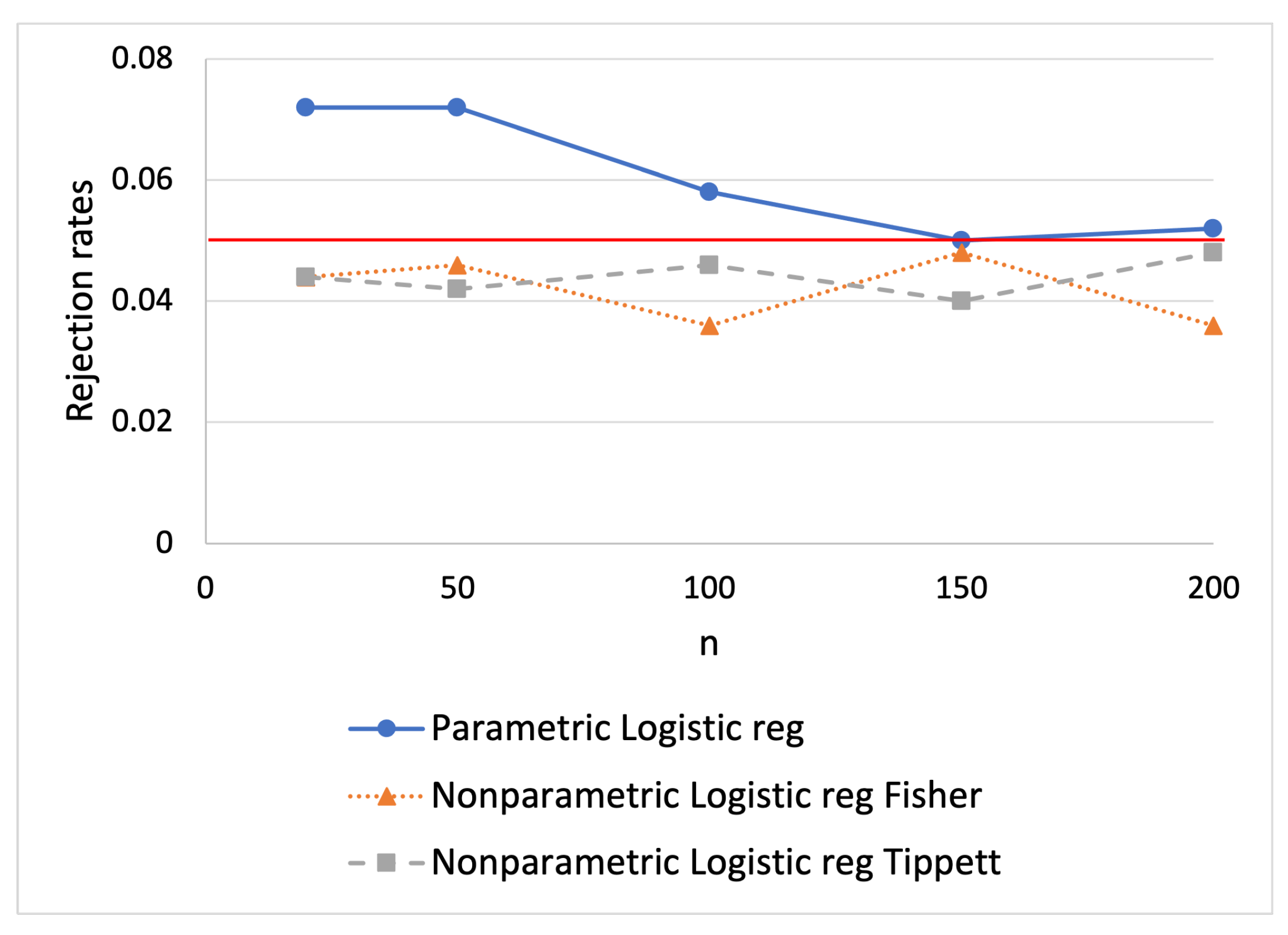
Firstly, simulations were carried out under the null hypothesis (), therefore and . Figure 1 reports the rejection rates of the compared tests as a function of the sample size n. As can be seen from the graphical representation, whilst the rejection rates of both the versions of the proposed non-parametric test (Fisher and Tippett combination) are almost always lower than the nominal level, for those of the parametric approach this is not always true, especially when the sample size is small. Hence, for small sample sizes, the parametric approach is anticonservative.
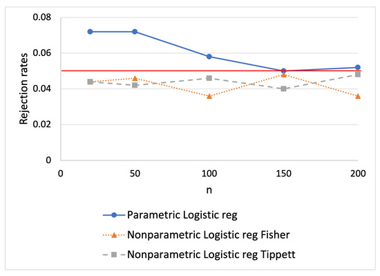
Figure 1.
Rejection rates of the parametric and nonparametric tests under as a function of n, with , , , , (represented by the red line).
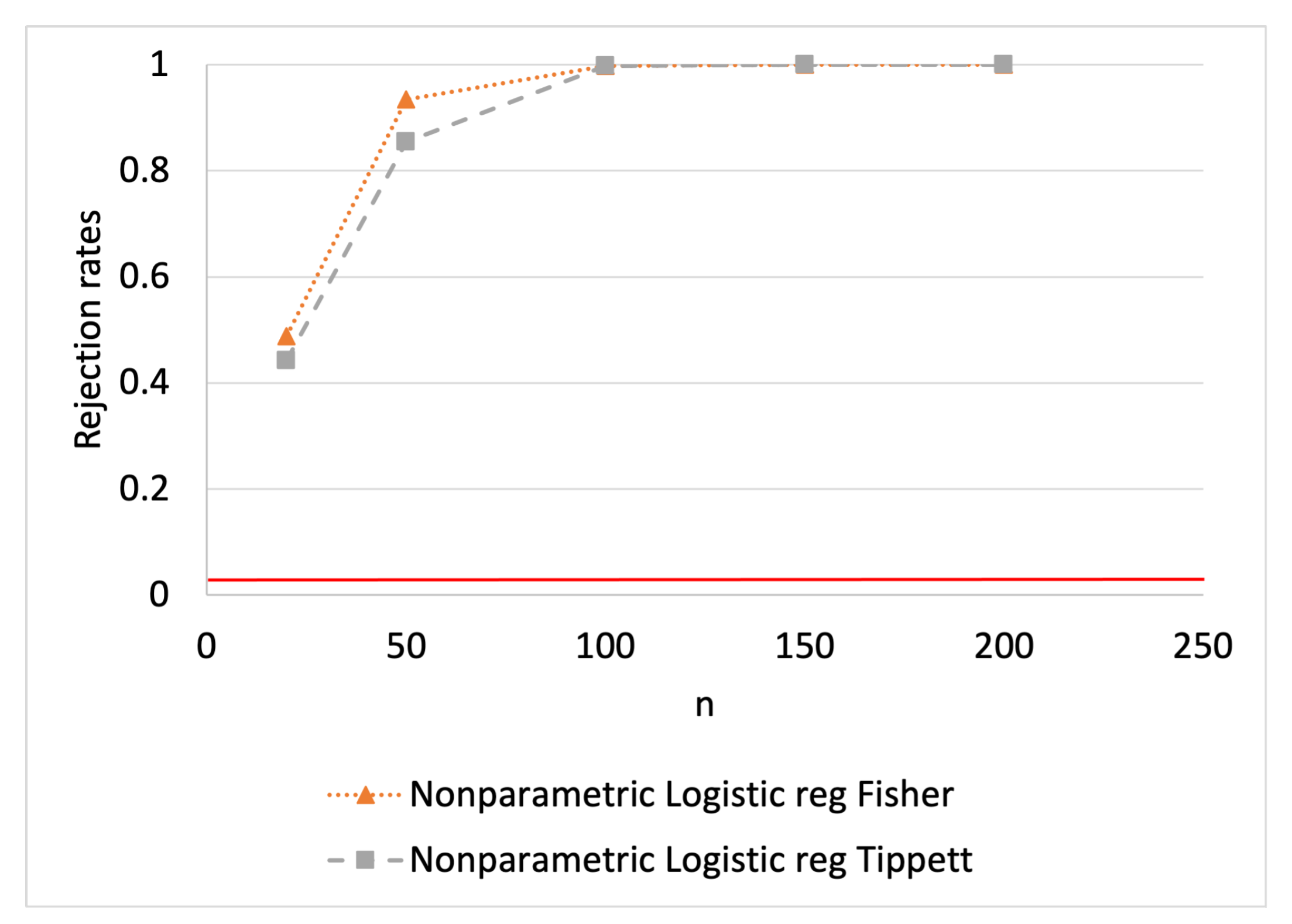
Subsequently, simulations were carried out under with . The power under , as a function of the sample size, is reported in Figure 2 to evaluate the consistency of the test. The test based on the combination of Fisher seems to be slightly more powerful. For both tests, the rejection rates under the alternative hypothesis exceed . Hence, both the tests are unbiased. As can be seen from the figure, the power increases as the sample size increases up to the convergence to 1 at . Hence, the consistency of the tests is illustrated.
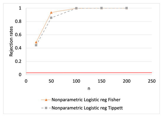
Figure 2.
Rejection rates of the nonparametric tests under as a function of n, with , , , , (represented by the red line).
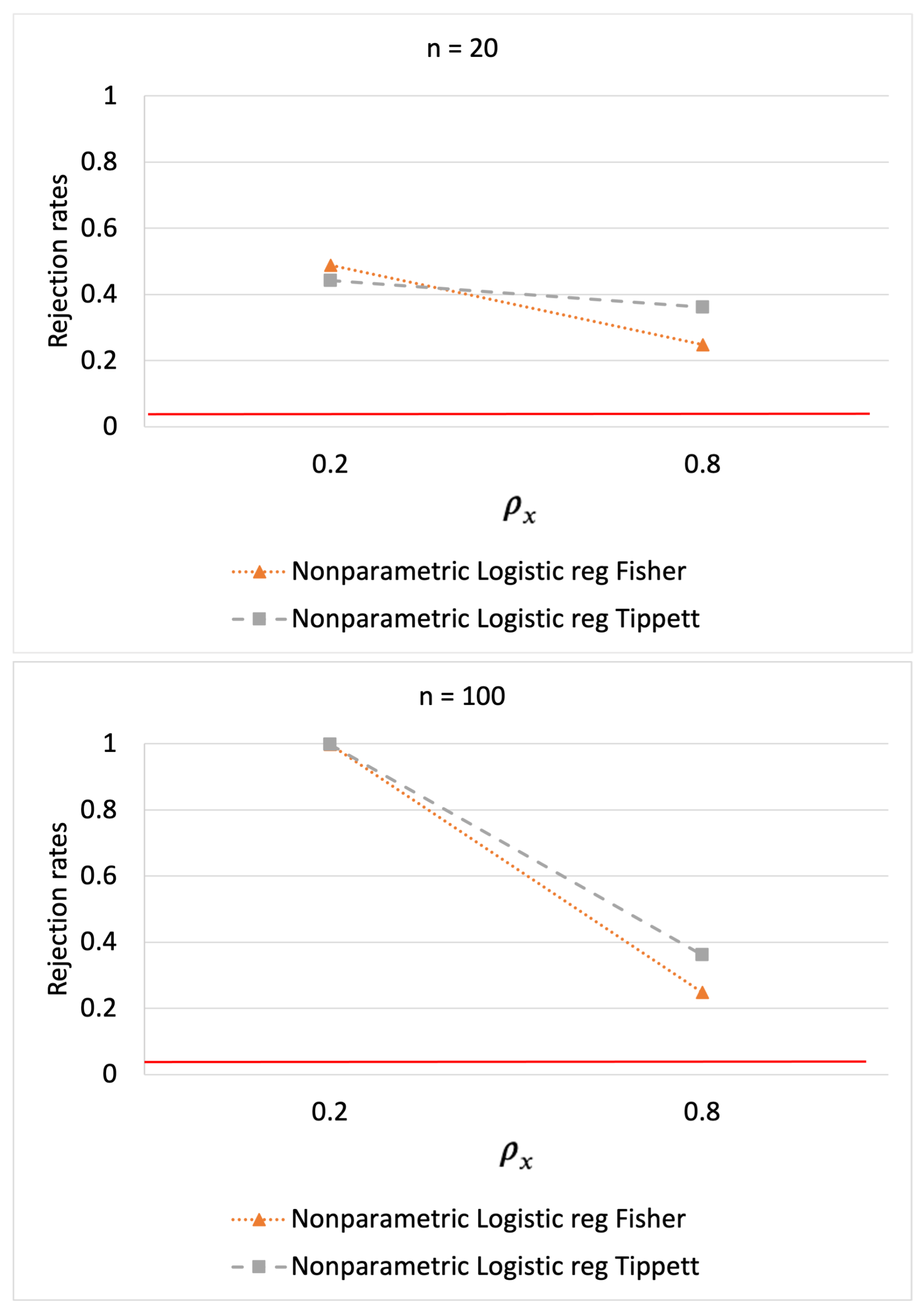
Furthermore, in Figure 3, the effect of the multicollinearity of the explanatory variables can be assessed. The rejection rates in the two cases of weak and strong correlations between the two predictors, i.e., and , respectively, are represented. It is noticeable that there is a significant decrease in power and a shift from weak to strong collinearity. The test based on the combination of Tippett seems to be less sensitive (hence more robust) to multicollinearity.
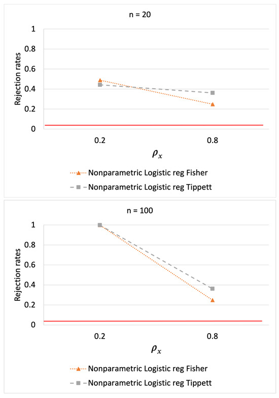
Figure 3.
Rejection rates of the nonparametric tests under as a function of , with and , , , , (represented by the red line).
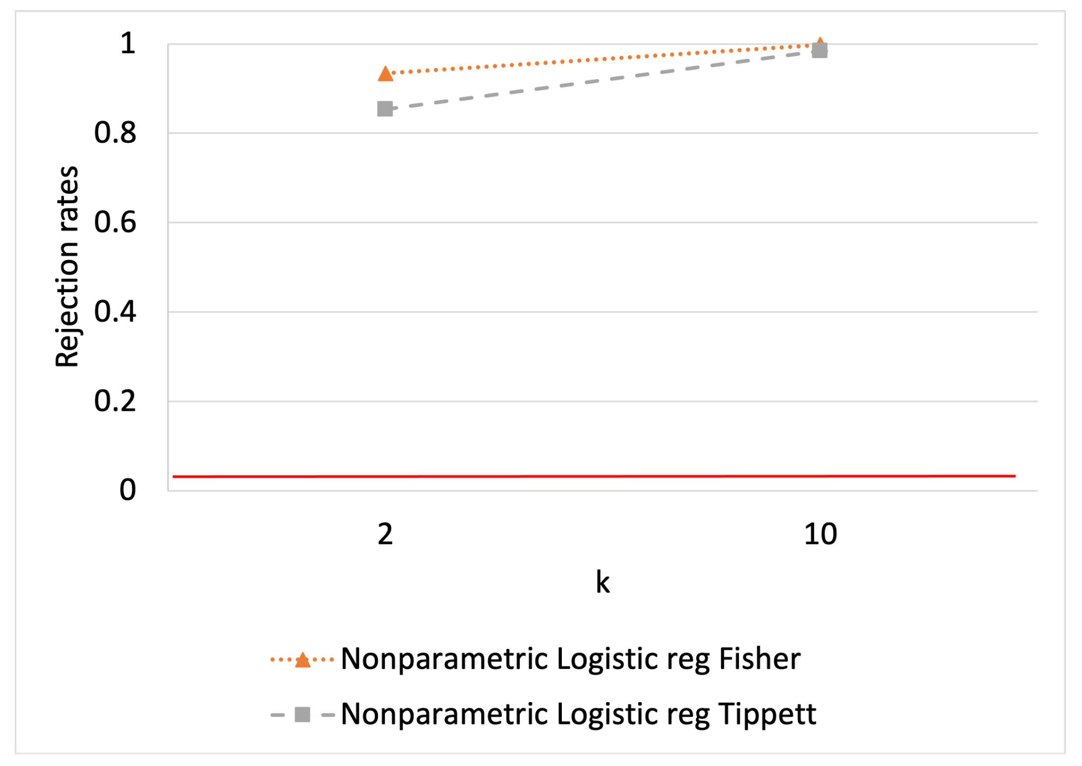
Finally, Figure 4 shows the rejection rates in the two cases of and . The power increases as the number of explanatory variables increases, so the finite sample consistency is proven.

Figure 4.
Rejection rates of the nonparametric tests under as a function of , with , , , , (represented by the red line).
5. Case Study
The case study concerns a statistical survey on the circular economy carried out in Italy in 2020. Specifically, it is related to technological innovation introduced in the two-year period from 2017 to 2018. The data relate to Italian SMEs operating in different sectors. The dataset is original and not publicly available. The data were collected through interviews carried out using the CATI method with a sample of Italian companies. It is worth noting that, in Section 4, the proposed nonparametric test was proven to be powerful for small samples, and it does not require asymptotic properties of the distribution of the test statistics to be satisfied, unlike parametric and other nonparametric methods. However, the method is very powerful, and therefore appropriate, even for large sample sizes, thanks to its consistency. As shown in Figure 2, the convergence to one of the powers can be reached for a sample size much smaller than that of the case study. Indeed, if the power tends to one for approximately , the test is certainly powerful when , even if we did not investigate the power behavior for such a large sample size. The companies were selected by a stratified random sampling method, and the final sample employed was composed of 3991 firms, excluding three outliers. Outliers were detected by using the classic rule based on the interquartile range . Data below and above were excluded. The variables considered are as follows:
- Response: a dichotomous variable that takes the value 1 if the answer to the question “Did the company introduce technological innovations of product or process in 2017–2018?” is “yes” and 0 if the answer is “no”.
- Explanatory variables:
- -
- The numeric variable size, which represents the number of employees of the firm,
- -
- The numeric variable age, which represents the number of years since the company was founded;
- -
- The dichotomous variable group, which indicates whether the company is part of a group (1: “yes” and 0: “no”);
- -
- Eight dichotomous variables that represent the firm’s sector.
The goal was to investigate the effect of the variables size, age, and group on the propensity to innovate. To overcome the possible confounding effect of the economic sector, we considered the eight binary variables representing the sectors in the set of predictors, which take the role of control variables. For the definition of the economic sectors, we grouped the sectors of the ATECO 2022 classification of the economic activities into eight categories. For the grouping of sectors, we took inspiration from [37]. For details about the definition of the strata with respect to the economic sectors, see Appendix B. The eight binary variables defined to represent the economic sectors are:
- food_bev: food products, beverages, and tobacco products,
- text_wear: textiles and wearing apparel,
- wood_print: wood, paper, printing, and reproduction,
- chem_plast: chemical-pharmaceutical, plastic and refined petroleum products, coke,
- metals: basic metals and fabricated metal products,
- comp_machinery: computer, electronic and optical products, machinery and equipment,
- motors: motor vehicles, trailers, semitrailers, and other transport equipment,
- other: other sectors.
As regards the composition of the dataset, the tables of descriptive statistics can be found in Appendix A. From Table A1, it can be seen that the average age of the companies is around 29 years, and the average size is 19 employees. From Table A2, we can deduce that the largest proportion of companies (26%) belong to the sector relating to basic metals and fabricated metal products, while the lowest percentage (2%) belong to the sector relating to motor vehicles, trailers, semi-trailers, and other transport equipment. Finally, Table A4 shows that the correlation between the predictors is particularly low.
The permutation test proposed and described in Section 3 was applied to the data to test the hypotheses defined in (7) at the significance level . In particular, we applied the test based on the Fisher combination. The overall p-value is equal to 0.0001, which indicates significance at the level . Since we have significance in the overall test, we consider the partial p-values related to the tests on the single coefficients. In Table 1, estimates and p-values of the partial tests on the regression coefficients are shown. According to the adjusted p-values, the significance of the overall test can be attributed only to some of the partial tests on the single coefficients [34,38]. In particular, the propensity to innovate seems to be related (with strong significance) to operating in the sector of chemical-pharmaceutical, plastic, refined petroleum products, and coke, in the sector of computer, electronics, and optical products, machinery, and equipment, and from age and size. All the significant coefficient estimates are positive, and this is consistent with the expected sign according to the economic theory, in all cases.

Table 1.
Estimates, unadjusted and adjusted p-values of the partial permutation tests on the regression coefficients of the univariate logistic regression model (significant estimates in bold).
The regression coefficients of the model were estimated using the maximum likelihood method. Before the parameter estimation, we computed the VIFs of all the explanatory variables to investigate the possible collinearity. All the VIFs were found to be less than 5, indicating that there is no multicollinearity issue for the data matrix of the explanatory variables (see Appendix A Table A3).
6. Results and Conclusions
The nonparametric solution proposed to test the goodness-of-fit of a logistic regression model is based on the combination of the permutation tests on the significance of the estimates of the single regression coefficients. This test, used jointly with the adjustment of the p-values of the partial tests on the coefficients for controlling the FWER for the multiplicity, is preferable to the classic parametric approach based on the separate application of the overall test on the whole model, and the single t-tests on the regression coefficients as is typical of the stepwise regression methods. The method is based on a procedure that takes into account the nature of multiple tests of the overall problem. It is distribution-free and consequently robust with respect to the departure from normality or other eventual assumed probability laws of the test statistics. Finally, it does not require that a specific dependence structure between the partial tests is assumed. Such a dependence is implicitly taken into account in the testing procedure and, specifically, in the permutation strategy. It incorporates in a unique procedure the test on the overall model and the test on the single regression coefficients, and it appears to be the most appropriate approach when the interest is both on the goodness-of-fit of the overall model and on the single regression coefficients [39].
Furthermore, the Monte Carlo simulation study confirms the validity of the proposed method and highlights its main limit related to the loss of power and the low convergence rate of the consistency in the case of high multicollinearity. Another limit of the proposed method concerns the performance when the conditions for the application of parametric methods are satisfied. Under these conditions, the proposed permutation test is less powerful (although only slightly) and therefore the parametric approach is preferable. A third limit concerns the Bonferroni–Holm p-value correction approach. This approach is preferable to others, but is still very conservative and causes many partial test significances to be lost. However, despite these limitations, the proposed test is well-approximated, unbiased, consistent, and powerful (with large and small sample sizes).
Regarding the case study, it is evident that some factors do not affect the propensity to innovate. For instance, this is the case of some specific sectors such as food and beverage products, textiles and wearing apparel, wood, paper and printing, metals, and motor vehicles. Furthermore, belonging to a group of companies does not seem to affect the propensity to innovate.
In conclusion, we contributed to the empirical literature about firms’ characteristics affecting the propensity to innovate. The propensity to innovate seems to be affected by age and size, and it is significantly higher in the sectors of chemical-pharmaceutical, plastic, refined petroleum products, and coke, and computer, electronic and optical products, machinery, and equipment. The findings are consistent with the empirical evidence provided by the studies cited in the literature review in the Introduction. These results suggest that bigger and more experienced companies have a higher inclination to implement technological innovations of products or processes. All the estimates of the coefficients found to be significant are positive, which means that the corresponding explanatory variables positively influence the propensity to innovate, in line with the aforementioned literature (see [4,5,6]).
In our opinion, such results represent a good starting point for the study of the relationship between firms’ characteristics or sectors of activity and their propensity to innovate. Without claiming to have fully explained the phenomenon, we believe that this model and these results can represent a step forward in the study of this subject, and can serve as a reference for other studies based on better models and a wider set of variables. Possible extensions and developments of this work concern, above all, the definition of more powerful tests both in terms of new partial test statistics and different combinations. A further development concerns the identification of less conservative p-value correction methods or effective non-parametric model selection techniques that can overcome the limitations of stepwise methods. Finally, it may be of interest to evaluate the robustness of the method with respect to outliers and, consequently, develop valid solutions for this problem.
Author Contributions
The authors contributed equally to this paper. Conceptualization, S.B. and M.B.; methodology, S.B. and M.B.; software, S.B. and M.B.; validation, S.B. and M.B.; formal analysis, S.B. and M.B.; investigation, S.B. and M.B.; resources, S.B. and M.B.; data curation, S.B. and M.B.; writing—original draft preparation, S.B. and M.B.; writing—review and editing, S.B. and M.B.; visualization, S.B. and M.B.; supervision, S.B. and M.B.; project administration, S.B. and M.B.; funding acquisition, S.B. and M.B. All authors have read and agreed to the published version of the manuscript.
Funding
This research received no external funding.
Data Availability Statement
Data will be made available upon request.
Acknowledgments
Authors thank the Italian Ministry of Education, University and Research that funded the departmental development program (DEM—University of Ferrara) for the period 2018–2022, to promote excellence in education and research (“Dipartimenti di Eccellenza”). This paper represents one output of such a project. The authors would like to thank the editor for the support and attention, and the anonymous reviewers as well for the valuable comments and suggestions that provided a relevant contribution to the improvement of the quality of the paper.
Conflicts of Interest
The authors declare no conflicts of interest.
Appendix A
Table A1.
Summary statistics of the two discrete explanatory variables.
Table A1.
Summary statistics of the two discrete explanatory variables.
| Firm’s Age | Firm’s Dimension | |
|---|---|---|
| Min | 1.00 | 0.00 |
| First quartile | 14.00 | 12.00 |
| Median | 28.00 | 15.00 |
| Mean | 28.75 | 18.85 |
| Third quartile | 40.00 | 22.00 |
| Max | 82.00 | 57.00 |
| Std. deviation | 16.99 | 10.91 |
Table A2.
Proportion over the sample of dummies explanatory variables.
Table A2.
Proportion over the sample of dummies explanatory variables.
| Variables | Proportion |
|---|---|
| food_bev | 0.10423 |
| text_wear | 0.08569 |
| wood_print | 0.09121 |
| chem_plast | 0.08093 |
| metals | 0.26109 |
| comp_machinery | 0.12704 |
| motors | 0.02055 |
| group | 0.09095 |
Table A3.
Variance Inflation Factor of the explanatory variables.
Table A3.
Variance Inflation Factor of the explanatory variables.
| Variables | VIF |
|---|---|
| food_bev | 1.31385 |
| text_wear | 1.25744 |
| wood_print | 1.28241 |
| chem_plast | 1.25353 |
| metals | 1.59205 |
| comp_machinery | 1.34693 |
| motors | 1.06982 |
| group | 1.07204 |
| age | 1.01615 |
| dimension | 1.05823 |
Table A4.
Correlation matrix between predictors.
Table A4.
Correlation matrix between predictors.
| Food | Textiles | Wood | Chemical | Metals | Computer | Motor | Group | Age | Dimension | |
|---|---|---|---|---|---|---|---|---|---|---|
| food | 1.000 | |||||||||
| textiles | −0.104 | 1.000 | ||||||||
| wood | −0.108 | −0.097 | 1.000 | |||||||
| chemical | −0.101 | −0.091 | −0.094 | 1.000 | ||||||
| metals | −0.202 | −0.182 | −0.118 | −0.176 | 1.000 | |||||
| computer | −0.130 | −0.117 | −0.121 | −0.113 | −0.227 | 1.000 | ||||
| motor | −0.049 | −0.044 | −0.046 | −0.043 | −0.086 | −0.055 | 1.000 | |||
| group | −0.014 | −0.069 | −0.036 | 0.111 | −0.033 | 0.073 | 0.016 | 1.000 | ||
| age | 0.029 | −0.017 | 0.048 | 0.003 | 0.027 | 0.016 | −0.038 | −0.075 | 1.000 | |
| dimension | −0.023 | −0.020 | −0.020 | 0.077 | −0.029 | 0.059 | 0.060 | 0.231 | 0.022 | 1.000 |
Appendix B. Unification of Sectors
Stratification of sectors defined according to the ATECO 2022 classification:
- food_bev: food products, beverages, and tobacco products (sectors 10-11-12 of the Ateco classification)
- text_wear: textiles and wearing apparel (sectors 13-14 of the Ateco classification)
- wood_print: wood, paper, printing and reproduction (sectors 16-17-18 of the Ateco classification)
- chem_plast: chemical-pharmaceutical, plastic and refined petroleum products, coke (sectors 19-20-21-22 of the Ateco classification)
- metals: basic metals and fabricated metal products (sectors 24-25 of the Ateco classification)
- comp_machinery: computer, electronic and optical products, machinery and equipment (sectors 26-28 of the Ateco classification)
- motors: motor vehicles, trailers, semitrailers, and other transport equipment (sectors 29-30 of the Ateco classification)
- other: other (sectors 8-15-23-27-31-32-33-43-46-47-73-95 of the Ateco classification)
References
- Maziriri, E.T.; Maramura, T.C. Green innovation in SMEs: The impact of green product and process innovation on achieving sustainable competitive advantage and improved business performance. Acad. Entrep. J. 2022, 28, 1–14. [Google Scholar]
- Shao, X.; Zhong, Y.; Liu, W.; Li, R.Y.M. Modeling the effect of green technology innovation and renewable energy on carbon neutrality in N-11 countries? Evidence from advance panel estimations. J. Environ. Manag. 2021, 296, 113189. [Google Scholar] [CrossRef] [PubMed]
- Li, G.; Xue, Q.; Qin, J. Environmental information disclosure and green technology innovation: Empirical evidence from China. Technol. Forecast. Soc. Chang. 2022, 176, 121453. [Google Scholar] [CrossRef]
- Sulisnaningrum, E.; Widarni, E.L.; Bawono, S. Causality relationship between human capital, technological development and economic growth. J. Manag. Econ. Ind. Organ. 2022, 6, 1–12. [Google Scholar] [CrossRef]
- Salimi, M.; Della Torre, E. Pay incentives, human capital and firm innovation in smaller firms. Int. Small Bus. J. 2022, 40, 507–530. [Google Scholar] [CrossRef]
- Rizos, V.; Behrens, A.; Van der Gaast, W.; Hofman, E.; Ioannou, A.; Kafyeke, T.; Flamos, A.; Rinaldi, R.; Papadelis, S.; Hirschnitz-Garbers, M.; et al. Implementation of circular economy business models by small and medium-sized enterprises (SMEs): Barriers and enablers. Sustainability 2016, 8, 1212. [Google Scholar] [CrossRef]
- Malik, A.; Sharma, P.; Vinu, A.; Karakoti, A.; Kaur, K.; Gujral, H.S.; Munjal, S.; Laker, B. Circular economy adoption by SMEs in emerging markets: Towards a multilevel conceptual framework. J. Bus. Res. 2022, 142, 605–619. [Google Scholar] [CrossRef]
- Gennari, F. The transition towards a circular economy. A framework for SMEs. J. Manag. Gov. 2022, 27, 1423–1457. [Google Scholar] [CrossRef]
- Yin, C.; Paz Salmador, M.; Li, D.; Begoña Lloria, M. Green entrepreneurship and SME performance: The moderating effect of firm age. Int. Entrep. Manag. J. 2022, 18, 255–275. [Google Scholar] [CrossRef]
- Nameroff, T.J.; Garant, R.J.; Albert, M.B. Adoption of green chemistry: An analysis based on US patents. Res. Policy 2004, 33, 959–974. [Google Scholar] [CrossRef]
- Radonjic, G.; Tominc, P. The role of environmental management system on introduction of new technologies in the metal and chemical/paper/plastics industries. J. Clean. Prod. 2007, 15, 1482–1493. [Google Scholar] [CrossRef]
- Austin, A.; Rahman, I.U. A triple helix of market failures: Financing the 3Rs of the circular economy in European SMEs. J. Clean. Prod. 2022, 361, 132284. [Google Scholar] [CrossRef]
- Pearson, K. “Das fehlergesetz und seine verallgemeiner-ungen durch fechner und pearson” a rejoinder. Biometrika 1905, 4, 169–212. [Google Scholar] [CrossRef]
- Pesarin, F. Multivariate Permutation Tests with Applications in Biostatistics; Wiley: Chichester, UK, 2001. [Google Scholar]
- Potter, D.M. A permutation test for inference in logistic regression with small- and moderate-sized datasets. Stat. Med. 2005, 24, 693–708. [Google Scholar] [CrossRef]
- Werft, W.; Benner, A. glmperm: A Permutation of Regressor Residuals Test for Inference in Generalized Linear Models. R J. 2010, 2, 39. [Google Scholar] [CrossRef]
- Gagnon-Bartsch, J.; Shem-Tov, Y. The classification permutation test: A flexible approach to testing for covariate imbalance in observational studies. Ann. Appl. Stat. 2019, 13, 1464–1483. [Google Scholar] [CrossRef]
- Cox, D.R. The Analysis of Binary Data; Methuen: London, UK, 1970. [Google Scholar]
- Conroy, B.; Sajda, P. Fast, Exact Model Selection and Permutation Testing for l2-Regularized Logistic Regression. JMLR Workshop Conf. Proc. 2012, 22, 246–254. [Google Scholar]
- Hirji, K.F.; Mehta, R.C.; Patel, N.R. Computing Distributions for Exact Logistic Regression. J. Am. Stat. Assoc. 1987, 82, 1110–1117. [Google Scholar] [CrossRef]
- Mehta, C.R.; Patel, N.R. Exact logistic regression: Theory and examples. Stat. Med. 1995, 14, 2143–2160. [Google Scholar] [CrossRef]
- Tabachnick, B.G.; Fidell, L.S. Using Multivariate Statistics, 4th ed.; Allyn and Bacon: Needham Heights, MA, USA, 2001. [Google Scholar]
- Pitman, E.J.G. Significance tests which may be applied to samples from any populations. III. J. R. Stat. Soc. Ser. Stat. Methodol. 1937, 4, 322–335. [Google Scholar]
- Pesarin, F.; Salmaso, L. Permutation Tests for Complex Data: Applications and Software; Wiley Series in Probability and Statistics; Wiley: Hoboken, NJ, USA, 2010. [Google Scholar]
- Giacalone, M.; Agata, Z.; Cozzucoli, P.C.; Alibrandi, A. Bonferroni-Holm and permutation tests to compare health data: Methodological and applicative issues. BMC Med. Res. Methodol. 2018, 18, 81. [Google Scholar] [CrossRef] [PubMed]
- Giacalone, M.; Alibrandi, A. A non parametric approach for the study of the controls in the production of agribusiness products. Electron. J. Appl. Stat. Anal. 2011, 4, 235–244. [Google Scholar]
- Alibrandi, A.; Giacalone, M.; Zirilli, A. Psychological stress in nurses assisting Amyotrophic Lateral Sclerosis patients: A statistical analysis based on Non-Parametric Combination test. Mediterr. J. Clin. Psychol. 2022, 10, 40. [Google Scholar]
- Bonnini, S.; Assegie, G.M. Advances on Permutation Multivariate Analysis of Variance for Big Data. Stat. Transit. 2022, 23, 163–183. [Google Scholar] [CrossRef]
- Bonnini, S. Testing for heterogeneity with categorical data: Permutation solution vs. bootstrap method. Commun. Stat.-Theory Methods 2014, 43, 906–917. [Google Scholar] [CrossRef]
- Bonnini, S.; Borghesi, M. Relationship between Mental Health and Socio-Economic, Demographic and Environmental Factors in the COVID- 19 Lockdown Period-A Multivariate Regression Analysis. Mathematics 2022, 10, 3237. [Google Scholar] [CrossRef]
- Giacalone, M.; Alibrandi, A. Overview and main advances in permutation tests for linear regression models. J. Math. Syst. Sci. 2015, 5, 53–59. [Google Scholar]
- Bonnini, S.; Cavallo, G. A study on the satisfaction with distance learning of university students with disabilities: Bivariate regression analysis using a multiple permutation test. Stat. Appl.-Ital. J. Appl. Stat. 2021, 33, 143–162. [Google Scholar]
- Bonnini, S.; Corain, L.; Marozzi, M.; Salmaso, L. Nonparametric Hypothesis Testing, Rank and Permutation Methods with Applications in R; Wiley: Hoboken, NY, USA, 2014. [Google Scholar]
- Westfall, P.H.; Young, S.S. On adjusting p-values for Multiplicity. Biometrics 1992, 49, 941–945. [Google Scholar] [CrossRef]
- Westfall, P.H. Kurtosis as peakedness, 1905–2014. “r.i.p.”. Am. Stat. Assoc. 2014, 68, 191–195. [Google Scholar] [CrossRef]
- Bonnini, S.; Assegie, G.M.; Trzcinska, K. Review about the Permutation Approach in Hypothesis Testing. Mathematics 2024, 12, 2617. [Google Scholar] [CrossRef]
- Dimitar, N. The impact of Foreign Direct Investments on employment: The case of the Macedonian manufacturing sector. East. J. Eur. Stud. 2017, 8, 147–165. [Google Scholar]
- Westfall, P.H.; Young, S.S. p-value adjustments for multiple tests in multivariate binomial models. J. Am. Stat. Assoc. 1989, 84, 780–786. [Google Scholar] [CrossRef]
- Das, P. Linear regression model: Goodness of fit and testing of hypothesis. In Econometrics in Theory and Practice: Analysis of Cross Section, Time Series and Panel Data with Stata; Springer: Singapore, 2018; pp. 75–108. [Google Scholar]
Disclaimer/Publisher’s Note: The statements, opinions and data contained in all publications are solely those of the individual author(s) and contributor(s) and not of MDPI and/or the editor(s). MDPI and/or the editor(s) disclaim responsibility for any injury to people or property resulting from any ideas, methods, instructions or products referred to in the content. |
© 2024 by the authors. Licensee MDPI, Basel, Switzerland. This article is an open access article distributed under the terms and conditions of the Creative Commons Attribution (CC BY) license (https://creativecommons.org/licenses/by/4.0/).