Finite-Time Asynchronous H_∞ Control for Non-Homogeneous Hidden Semi-Markov Jump Systems

Abstract

This article explores the finite-time control problem associated with a specific category of non-homogeneous hidden semi-Markov jump systems. Firstly, a hidden semi-Markov model is designed to characterize the asynchronous interactions that occur between the true system mode and the controller mode, and emission probabilities are used to establish relationships between system models and controller modes. Secondly, a novel piecewise homogeneous method is introduced to tackle the non-homogeneous issue by taking into account the time-dependent transition rates for the jump rules between different modes of the system. Thirdly, an asynchronous controller is developed by applying Lyapunov theory along with criteria for stochastic finite-time boundedness, ensuring the specified $H_{\infty }$ performance level is maintained. Finally, the effectiveness of this method is verified through two simulation examples.

1. Introduction

The Markov process (MP) is commonly utilized to analyze system state transitions in various fields such as finance, power systems, and robotics. Due to its ability to capture dynamic behavior, Markov jump systems (MJSs) have been extensively researched in recent years [1,2,3,4,5]. In continuous-time systems, the transition rates between different modes of an MP are influenced solely by the current mode in which the system resides. The dwell time (DT) follows an exponential distribution. In real systems, the DT distribution often follows different patterns, and new methods need to be explored to solve this problem. Unlike a traditional MP, semi-Markov processes (SMPs) consider historical data, and the DT is not constrained by an exponential distribution. As a result, researchers and practitioners may find semi-Markov jump systems (SMJSs) to be more suitable for modeling a variety of systems where the exponential assumption does not hold, thus enhancing their applicability in complex scenarios [6,7,8,9,10,11,12]. Regarding the stability analysis and synthesis of semi-Markov jump systems, Ref. [13] focused on the issues of stochastic stability and stabilization regarding a particular category of continuous-time semi-Markovian jump systems that feature mode transition-dependent sojourn time distributions. In [14], the author discussed the problem of $H_{\infty }$ observer-based control for a class of continuous-time semi-Markovian jump systems with more detailed observational information.

A significant limitation in the majority of current research is the assumption that transition rates (TRs) are constant over time. This perspective overlooks the dynamic nature of many practical engineering applications. For instance, in contexts such as manufacturing systems and voltage conversion circuitry, the conditions and factors affecting TRs frequently change, rendering the assumption of time invariance unrealistic. Therefore, it is important to consider non-homogeneous semi-Markov jump systems (NHSMJSs) in these scenarios. Ref. [15] proposed an SMP framework that is affected by deterministic high-order switching signals, and the Markov renewal process is non-homogeneous. The stabilization problem of a class of stochastic NHSMJSs is studied in [16]. To date, there is limited research on NHSMJSs, making it a fruitful area for exploration. This lack of existing literature is a key driving factor behind the current study.

On the other hand, the above research is based on the synchronization of the system mode and the controller mode. In fact, the asynchronous problem of SMJSs has attracted widespread attention from researchers. Given the potential misalignment of variables and modes between the filter and plant in real network environments, a double asynchronous phenomenon may occur. For this reason, Ref. [17] proposed a new fault detection filter which specifically targets fault detection in fuzzy SMJSs. Ref. [18] explored the issue of asynchronous control in two-dimensional SMJSs within the Roesser model. The interval type-2 fuzzy model was investigated in [19], which developed an asynchronous sliding mode control mechanism to achieve a quasi-sliding mode, effectively addressing the challenges posed by parameter uncertainties for nonlinear semi-Markov jump models. Hidden semi-Markov jump systems (HSMJSs) have emerged as a research area with the potential to overcome the limitations of the assumption that the system mode is consistent with the controller [20,21,22,23,24]. The hidden semi-Markov process (HSMP) can be understood as a parameter process characterized by two variables. The stochastic process, referred to as the SMP, is time-homogeneous and remains undisclosed to the controller, making it hidden. The observed modes within the underlying process are determined from the emission probabilities of the actual and observed system modes, which aids in the identification of hidden system modes. While there has been significant research on stability analysis and controller synthesis for HSMJSs, certain areas within this field have not been fully explored, leaving open questions that have inspired our current investigation.

Building upon this foundation, the examination of stability and control mechanisms for non-homogeneous hidden semi-Markov jump systems is undertaken. Ref. [25] addresses the analysis of stability for a class of discrete-time non-homogeneous hidden semi-Markov jump systems that operate with limited information regarding the sojourn time probability density functions. Ref. [26] explores the non-fragile asynchronous control challenge within discrete-time non-homogeneous hidden semi-Markov Lur’e systems, which face uncertainties related to the system mode and gain. However, the aforementioned studies are primarily based on discrete-time scenarios. To the best of the author’s knowledge, the stability analysis of continuous-time non-homogeneous hidden semi-Markov jump systems remains unexplored. This gap in the literature serves as one of the primary motivations for this article.

Meanwhile, in numerous engineering applications, the performance during a transition phase of a system is evaluated within a restricted operational time frame, contrasting with the analysis of stability over an endless duration. The goal of finite-time stability is to guarantee that, within a specified time frame, the system’s trajectories do not surpass a certain physical limit. Up to this point, significant interest has been directed towards finite-time stability [12,27,28].

This study examines the design challenges associated with asynchronous $H_{\infty }$ controllers for non-homogeneous HSMJSs within a finite-time framework. The main contributions of this research can be outlined as follows:

(i) A hidden semi-Markov model is proposed to describe the asynchronous behavior observed between the mode of the actual system and that of the controller.

(ii) A novel piecewise homogeneous approach is suggested for addressing the non-homogeneous phenomenon by taking into account the time-dependent transition rates of the jump rules across different system modes.

(iii) An asynchronous controller is designed using Lyapunov theory to generate finite stochastic criteria with the prescribed $H_{\infty }$ performance level.

Table 1. Common notations in this paper.

Notations	Meanings
${\mathbb{R}}^n$	n-dimensional Euclidean space
$\Vert ·\Vert$	Euclidean norm
$U>0$	U is a positive-definite symmetric matrix
$U^{\mathrm{T}}$	the transpose of U
$U^{-1}$	the inverse of U
${\lambda }_{max}\left\{U\right\}$, ${\lambda }_{min}\left\{U\right\}$	maximum and minimum eigenvalues of U
$\mathbf{He}\left\{U\right\}$	U + $U^{\mathrm{T}}$
$E(·)$	the mathematical expectation
∗	the elision for symmetry matrix
${\mathcal{M}}_1$	1,2, …$M_1$
${\mathcal{M}}_2$	1,2, …$M_2$
$\mathcal{N}$	1,2, …N

lists the notations used in this article.

2. Materials and Methods

We consider a class of non-homogeneous HMJSs described by

$$\begin{array}{c}\hfill \left\{\begin{array}{c}\dot{x}\left(t\right)=A_{r_t}x\left(t\right)+B_{r_t}u\left(t\right)+C_{r_t}\omega \left(t\right),\hfill \\ z\left(t\right)=D_{r_t}x\left(t\right)\hfill \end{array}\right.\end{array}$$

(1)

where $x\left(t\right)\in {\mathbb{R}}^n$ represents the state vector of the system, $u\left(t\right)\in {\mathbb{R}}^m$ represents the control input, $z\left(t\right)\in {\mathbb{R}}^p$ represents the measured output, and $\omega \left(t\right)\in {\mathbb{R}}^q$ represents the external disturbance belonging to $L_2[0,\infty )$, $\forall t\ge 0$. $r_t$ represents a continuous-time non-homogeneous semi-Markov process that assumes values within the set ${\mathcal{M}}_1$. The time-dependent TRs are indicated as follows:

$$\mathbf{Pr}\{r_{t+\mathsf{\Delta }}=j\mid r_t=i\}=\left\{\begin{array}{cc}{\pi }_{ij}^{{\theta }_t}\left(\delta \right)\mathsf{\Delta }+o\left(\mathsf{\Delta }\right),\hfill & j\ne i,\hfill \\ 1+{\pi }_{ii}^{{\theta }_t}\left(\delta \right)\mathsf{\Delta }+o\left(\mathsf{\Delta }\right),\hfill & j=i.\hfill \end{array}\right.$$

(2)

with $\mathsf{\Delta }>0$, where $\delta$ means sojourn time, and $\underset{\mathsf{\Delta }\to 0}{lim}o\left(\mathsf{\Delta }\right)/\mathsf{\Delta }=0$, ${\pi }_{ij}^{{\theta }_t}\left(\delta \right)>0$$(i,j\in {\mathcal{M}}_1,j\ne i)$ is the transition rate between the i mode at time t and the j mode at time $t+\mathsf{\Delta }$, which satisfies

$$\begin{array}{c}\hfill {\pi }_{ii}^{{\theta }_t}\left(\delta \right)=-\sum _{j\in {\mathcal{M}}_1\setminus \left\{i\right\}}{\pi }_{ij}^{{\theta }_t}\left(\delta \right),\forall i\in {\mathcal{M}}_1.\end{array}$$

In this context, the variable ${\theta }_t$ represents a piecewise constant switching signal that assumes values from the set $\mathcal{N}$, and it determines the pattern of the transition probability matrix at each moment. For every potential value of the variable $r_t=i$, with ${\theta }_t=p$, the TRs, ${\pi }_{ij}^p$, are formulated as a function of the high-level switching signal, ${\theta }_t=p$.

This formulation underscores the fact that the TRs exhibit temporal variability. Additionally, when organized sequentially, the matrix representing the TRs is introduced as

$$\begin{array}{c}\hfill {\mathsf{\Pi }}^p\left(\delta \right)=\left[\begin{array}{ccc}{\pi }_{11}^p\left(\delta \right)& {\pi }_{12}^p\left(\delta \right)& \cdots {\pi }_{1m}^p\left(\delta \right)\\ {\pi }_{21}^p\left(\delta \right)& {\pi }_{22}^p\left(\delta \right)& \cdots {\pi }_{2m}^p\left(\delta \right)\\ ⋮& ⋮& ⋮\\ {\pi }_{m1}^p\left(\delta \right)& {\pi }_{m2}^p\left(\delta \right)& \cdots {\pi }_{mm}^p\left(\delta \right)\end{array}\right]\end{array}$$

Due to asynchronous phenomenon, we cannot assume that the controller has precise access to modal system information. This study aimed to discover the hidden controller modes by utilizing an observed mode analysis approach. Figure 1 can provide a clearer depiction of the HSMP. $\{r_t,t\ge 0\}$ stands for the hidden system mode, and the observed mode $\{{\sigma }_t,t\ge 0\}$ assumes values from the set ${\mathcal{M}}_2$. A range of observed modes can be emitted by each hidden system mode. The emission probability matrix is

$$\begin{array}{c}\hfill \mathbf{Pr}\{{\sigma }_t=m\mid r_t=i\}={\rho }_{im},\forall i\in {\mathcal{M}}_1,m\in {\mathcal{M}}_2,\end{array}$$

(3)

with ${\rho }_{im}\in [0,1]$ and ${\sum }_{m\in {\mathcal{M}}_2}{\rho }_{im}=1$.

In this paper, for $r_t=i$, ${\theta }_t=p$, and ${\sigma }_t=m$, the parameter matrices $A_i$, $B_i$, $C_i$, and $D_i$ possess suitable dimensions. We consider the following three-variable-dependent asynchronous controller for non-homogeneous HSMJSs (1):

$$u\left(t\right)=K_{i,m,p}x\left(t\right),$$

(4)

where $K_{i,m,p}$ means the feedback control gain matrix. The combination of (1) and (4) gives rise to an expression for non-homogeneous HSMJS as follows:

$$\begin{array}{c}\hfill \left\{\begin{array}{c}\dot{x}\left(t\right)=(A_i+B_i{K}_{i,m,p})x\left(t\right)+C_i\omega \left(t\right),\hfill \\ z\left(t\right)=D_{i}x\left(t\right).\hfill \end{array}\right.\end{array}$$

(5)

Remark 1.

In practical application systems, the modal information acquired by the controller is often inaccurate, meaning that the true system model remains concealed from the controller. To address this issue, the variable ${\sigma }_t$ is proposed to denote the mode of the controller, with the relationship between $r_t$ and ${\sigma }_t$ illustrated by Equation (3).

Remark 2.

In actual systems, it is unrealistic to obtain the transition probability at each moment in real time. Therefore, it is difficult to study semi-Markov jump systems with time-varying transition probabilities, which also increases the difficulty of deriving the stability theory. Fortunately, in control practice, this type of system can usually be divided into a limited number of continuous homogeneous systems, hence the piecewise homogeneous system proposed in this article.

Before we continue, here are the definitions, given below.

Assumption A1

([27]). Given the time interval $[0,T]$ and the constant $d\ge 0$, the unknown external disturbance $\omega \left(t\right)$ satisfies the following conditions:

$$\begin{array}{c}\hfill {\int }_0^T{\omega }^{\mathrm{T}}\left(t\right)\omega \left(t\right)\mathrm{d}t⩽d^2.\end{array}$$

(6)

Definition 1

([29]). HSMJSs (5) are stochastically finite-time-bounded (SFTB) within a time interval $\left[0,T\right]$ concerning $(d,T,R,c_1,c_2)$ if the following conditions hold:

$$\begin{array}{c}\hfill \left\{\begin{array}{c}{\int }_0^T{\omega }^{\mathrm{T}}\left(t\right)\omega \left(t\right)dt⩽d^2,\hfill \\ x^{\mathrm{T}}\left(0\right)Rx\left(0\right)⩽c_1\Rightarrow \mathrm{E}\left\{x^{\mathrm{T}}\left(t\right)Rx\left(t\right)<c_2\right\},\forall t\in \{0,T\}.\hfill \end{array}\right.\end{array}$$

(7)

where $c_1$ and $c_2$ are positive scalars with $c_2>c_1$, and $R>0$ is a weighting matrix.

Definition 2

([29]). Given a scalar $\gamma \ge 0$, if there is an asynchronous controller (4) under zero initial conditions such that all $i\in {\mathcal{M}}_1$, $m\in {\mathcal{M}}_2$, and $p\in \mathcal{N}$, the HSMJS (5) is SFTB and satisfies the following:

$$\begin{array}{c}\hfill {\int }_0^T{z}^{\mathrm{T}}\left(t\right)z\left(t\right)dt<{\gamma }^2{\int }_0^T{\omega }^{\mathrm{T}}\left(t\right)\omega \left(t\right)dt.\end{array}$$

(8)

We say that the controller (4) satisfies the $H_{\infty }$ performance index γ.

3. Results

Theorem 1.

For a given scalar $\alpha >0$, the closed-loop non-homogeneous HSMJS (5) is SFTB and satisfies the $H_{\infty }$ performance index γ concerning $(d,T,R,c_1,c_2)$ if there exist symmetric matrices $P_{i,p}>0$, such that the following conditions hold for every value of $i\in {\mathcal{M}}_1$, $m\in {\mathcal{M}}_2$, and $p\in \mathcal{N}$:

$$e^{\alpha T}{c}_1{\lambda }_2+{\gamma }^2{d}^2-c_2{\lambda }_1<0$$

(9)

$$\mathsf{\Omega }=\left[\begin{array}{ccc}{\mathsf{\Xi }}_{11}& {\mathsf{\Xi }}_{12}& {\mathsf{\Xi }}_{13}\\ \ast & {\mathsf{\Xi }}_{22}& 0\\ \ast & \ast & {\mathsf{\Xi }}_{33}\end{array}\right]<0$$

(10)

with

$$\begin{array}{ccc}\hfill {\lambda }_1& =& {\lambda }_{min}\left\{R^{-{\displaystyle \frac{1}{2}}}{P}_{i,p}{R}^{-{\displaystyle \frac{1}{2}}}\right\},{\lambda }_2={\lambda }_{max}\left\{R^{-{\displaystyle \frac{1}{2}}}{P}_{i,p}{R}^{-{\displaystyle \frac{1}{2}}}\right\},\hfill \\ \hfill {\mathsf{\Xi }}_{11}& =& \mathbf{He}[P_{i,p}(A_i+\sum _{m\in {\mathcal{M}}_2}{\rho }_{im}{B}_i{K}_{i,m,p})]+\sum _{j\in {\mathcal{M}}_1}{\overline{\pi }}_{ij}^p{P}_{j,p}-\alpha P_{i,p}\hfill \\ \hfill {\mathsf{\Xi }}_{12}& =& P_{i,p}{C}_i,{\mathsf{\Xi }}_{13}=D_i^{\mathrm{T}},\hfill \\ \hfill {\mathsf{\Xi }}_{22}& =& -{\gamma }^2{e}^{-\alpha T},{\mathsf{\Xi }}_{33}=-I,\hfill \\ \hfill {\overline{\pi }}_{ij}^p& =& E\left[{\pi }_{ij}^p\left(\delta \right)\right]={\int }_0^{\infty }{\pi }_{ij}\left(\delta \right)d{\mathcal{F}}_i^p\left(\delta \right),\hfill \end{array}$$

where ${\mathcal{F}}_i^p\left(\delta \right)$ represents the probability density function of DT with respect to δ.

Proof of Theorem 1.

A stochastic Lyapunov functional candidate is chosen as follows:

$$V\left(x\left(t\right)\right)=x^{\mathrm{T}}{P}_{i,p}x\left(t\right).$$

(11)

Define $\mathcal{L}$ as a weak infinity operator, and for $\alpha >0$, the auxiliary function is defined as follows:

$$\begin{array}{c}\hfill J\left(t\right)=E\{\mathcal{L}V\left(x\left(t\right)\right)-\alpha V\left(x\left(t\right)\right)-{\gamma }^2{e}^{-\alpha T}{\omega }^{\mathrm{T}}\left(t\right)\omega \left(t\right)+z^{\mathrm{T}}\left(t\right)z\left(t\right)\}.\end{array}$$

(12)

By carrying out this calculation, we obtain

$$\begin{array}{ccc}\hfill J(t)& =& E\{\mathcal{L}V(x(t))-\alpha V(x(t))-{\gamma }^2{e}^{-\alpha T}{\omega }^{\mathrm{T}}(t)\omega (t)+z^{\mathrm{T}}(t)z(t)\}\hfill \\ & =& E\{x^{\mathrm{T}}(t)(\sum _{j\in {\mathcal{M}}_1}{\pi }_{ij}^p{P}_{j,p})x(t)+2[x^{\mathrm{T}}(t)P_{i,p}{A}_{i}x(t)\hfill \\ & +& x^{\mathrm{T}}(t)(\sum _{m\in {\mathcal{M}}_2}{\rho }_{im}{P}_{i,p}{B}_i{K}_{i,m,p})x(t)+{\omega }^{\mathrm{T}}(t)P_{i,p}{C}_i\omega (t)]\hfill \\ & -& \alpha V(x(t))-{\gamma }^2{e}^{-\alpha T}{\omega }^{\mathrm{T}}(t)\omega (t)+z^{\mathrm{T}}(t)z(t)\}.\hfill \end{array}$$

(13)

Thus, the following inequality can be obtained:

$$\begin{array}{c}\hfill J\left(t\right)\le {\eta }^{\mathrm{T}}\left(t\right)\mathsf{\Omega }\eta \left(t\right)\end{array}$$

(14)

where $\eta \left(t\right)={\left[x\left(t\right)\omega \left(t\right)\right]}^{\mathrm{T}}$. From condition (10), we obtain

$$\begin{array}{c}\hfill J\left(t\right)<0.\end{array}$$

(15)

According to (15), the equivalent inequality is obtained:

$$\mathcal{L}V\left(x\left(t\right)\right)-\alpha V\left(x\left(t\right)\right)-{\gamma }^2{e}^{-\alpha T}{\omega }^{\mathrm{T}}\left(t\right)\omega \left(t\right)+z^{\mathrm{T}}\left(t\right)z\left(t\right)<0.$$

(16)

Then, taking the expectation of (16), it follows that

$$E\left\{\mathcal{L}{e}^{-\alpha t}V\left(x\left(t\right)\right)\right\}<{\gamma }^2{e}^{-\alpha (t+T)}E\left\{{\omega }^{\mathrm{T}}\left(t\right)\omega \left(t\right)\right\}.$$

(17)

Integrating (17) over $t(t\in (0,T\left]\right)$ yields

$$\begin{array}{c}\hfill e^{-\alpha t}E\left\{V\left(x\left(t\right)\right)\right\}<E\left\{V\left(x\left(0\right)\right)\right\}+{\gamma }^{2}E\left\{{\int }_0^T{e}^{-\alpha (\tau +T)}{\omega }^{\mathrm{T}}\left(\tau \right)\omega \left(\tau \right)d\tau \right\}.\end{array}$$

(18)

Multiplying (18) by $e^{\alpha t}$ yields

$$\begin{array}{c}\hfill E\left\{V\left(x\left(t\right)\right)\right\}<e^{\alpha t}E\left\{V\left(x\left(0\right)\right)\right\}+{\gamma }^2{d}^2<e^{\alpha T}{\lambda }_2{c}_1+{\gamma }^2{d}^2.\end{array}$$

Since

$$\begin{array}{c}\hfill E\left\{V\left(x\left(t\right)\right)\right\}\ge {\lambda }_{1}E\left\{x^{\mathrm{T}}\left(t\right)Rx\left(t\right)\right\},\end{array}$$

We can obviously obtain

$$\begin{array}{c}\hfill E\left\{x^{\mathrm{T}}\left(t\right)Rx\left(t\right)\right\}<{\displaystyle \frac{e^{\alpha T}{\lambda }_2{c}_1+{\gamma }^2{d}^2}{{\lambda }_1}}.\end{array}$$

From (9), it follows that

$$E\left\{V\left(x\left(t\right)\right)\right\}<{\displaystyle \frac{e^{\alpha T}{\lambda }_2{c}_1+{\gamma }^2{d}^2}{{\lambda }_1}}<c_2.$$

Therefore, according to Definition 1, the closed-loop system (5) is SFTB. If we multiply (16) by $e^{\alpha t}$ and calculate the mathematical expectation, we obtain

$$\begin{array}{c}\hfill E\left\{\mathcal{L}\left[e^{-\alpha t}V\left(x\left(t\right)\right)\right]\right\}<E\left\{e^{-\alpha t}[{\gamma }^2{e}^{-\alpha T}{\omega }^{\mathrm{T}}\left(t\right)\omega \left(t\right)-z^{\mathrm{T}}\left(t\right)z\left(t\right)]\right\}.\end{array}$$

(19)

Integrating (19) over $t(t\in (0,t\left]\right)$ under zero initial conditions, we obtain

$$\begin{array}{c}\hfill E\left\{{\int }_0^T{e}^{-\alpha \ell }[z^{\mathrm{T}}(\ell )z(\ell )-{\gamma }^2{e}^{-\alpha T}{\omega }^{\mathrm{T}}(\ell )\omega (\ell )]d\ell \right\}<0.\end{array}$$

Thus, for all $t(t\in (0,T\left]\right)$, it follows that

$$\begin{array}{c}\hfill E\left\{{\int }_0^T{z}^{\mathrm{T}}\left(t\right)z\left(t\right)dt\right\}<e^{-\alpha T}E\left\{{\int }_0^T{\gamma }^2{\omega }^{\mathrm{T}}\left(t\right)\omega \left(t\right)dt\right\}<{\gamma }^{2}E\left\{{\int }_0^T{\omega }^{\mathrm{T}}\left(t\right)\omega \left(t\right)\right\}.\end{array}$$

Returning to Definition 2, the closed-loop system (5) is SFTB and satisfies the $H_{\infty }$ performance index $\gamma$. This completes the proof. □

The following theorem we solve for the three-variable-dependent asynchronous controller.

Theorem 2.

For a given scalar $\alpha >0$, the closed-loop non-homogeneous HSMJS (5) is SFTB and satisfies the $H_{\infty }$ performance index γ concerning $(d,T,R,c_1,c_2)$ if there exist symmetric matrices $P_{i,p}>0$ such that the following conditions hold for every value of $i\in {\mathcal{M}}_1$, $m\in {\mathcal{M}}_2$, and $p\in \mathcal{N}$:

$$\left[\begin{array}{cc}({\gamma }^2{d}^2-c_2{\lambda }_1)e^{-\alpha T}& \sqrt{c_1}\\ \ast & -{\lambda }_2\end{array}\right]<0$$

(20)

$$\tilde{\mathsf{\Omega }}=\left[\begin{array}{ccc}{\tilde{\mathsf{\Xi }}}_{11}& {\tilde{\mathsf{\Xi }}}_{12}& {\tilde{\mathsf{\Xi }}}_{13}\\ \ast & {\mathsf{\Xi }}_{22}& 0\\ \ast & \ast & {\mathsf{\Xi }}_{33}\end{array}\right]<0,$$

(21)

with

$$\begin{array}{ccc}\hfill {\tilde{\lambda }}_1& =& {\lambda }_{min}\left\{R^{-{\displaystyle \frac{1}{2}}}{X}_{i,p}{R}^{-{\displaystyle \frac{1}{2}}}\right\},{\tilde{\lambda }}_2={\lambda }_{max}\left\{R^{-{\displaystyle \frac{1}{2}}}{X}_{i,p}{R}^{-{\displaystyle \frac{1}{2}}}\right\},\hfill \\ \hfill {\tilde{\mathsf{\Xi }}}_{11}& =& \mathbf{He}[A_i{X}_{i,p}+\sum _{m\in {\mathcal{M}}_2}{\rho }_{im}{B}_i{N}_{i,m,p}]+\sum _{j\in {\mathcal{M}}_1}{\overline{\pi }}_{ij}^p{X}_{i,p}^{\mathrm{T}}{P}_{j,p}{X}_{i,p}-\alpha X_{i,p},\hfill \\ \hfill {\tilde{\mathsf{\Xi }}}_{12}& =& C_i,{\tilde{\mathsf{\Xi }}}_{13}=X_{i,p}^{\mathrm{T}}{D}_i^{\mathrm{T}}.\hfill \end{array}$$

The other parameters are consistent with Theorem 1. Then, the three-variable-dependent controller’s gain matrices are given as $K_{i,m,p}=N_{m,p}{X}_{i,p}^{-1}$.

Proof of Theorem 2.

Define

$$X_{i,p}=P_{i,p}^{-1},N_{i,m,p}=K_{i,m,p}{X}_{m,p},$$

$diag\{X_{i,p};I;I\}$, and its transposition; then, (10) is equivalent to (21), and, obviously, (9) is equivalent to (20). Proof completed. □

Remark 3.

In contrast to the asynchronous controllers commonly found in the existing literature, the asynchronous controller presented in this paper is defined by three variables. This approach leverages the characteristics of the system state more effectively, thereby significantly reducing conservatism.

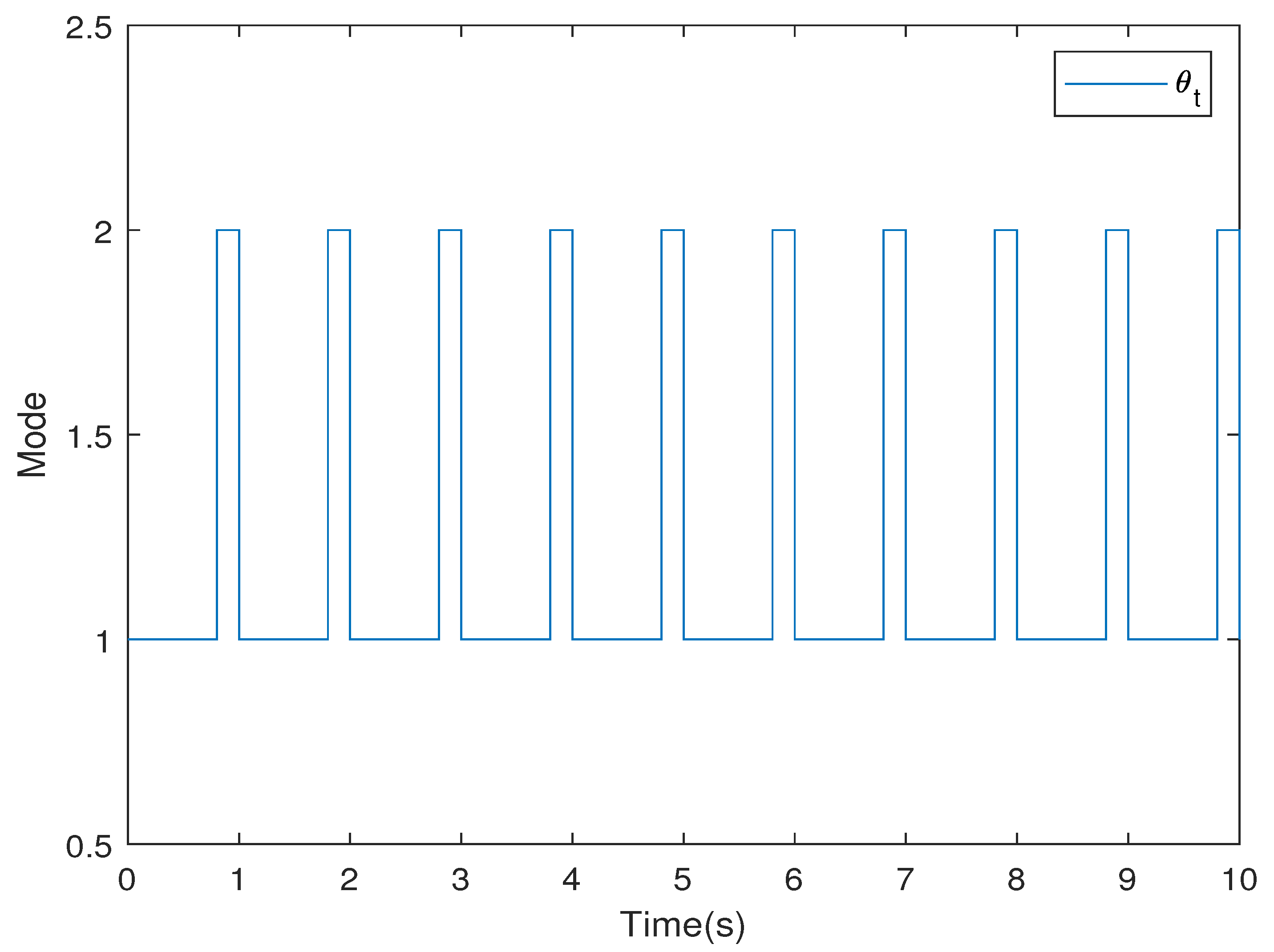
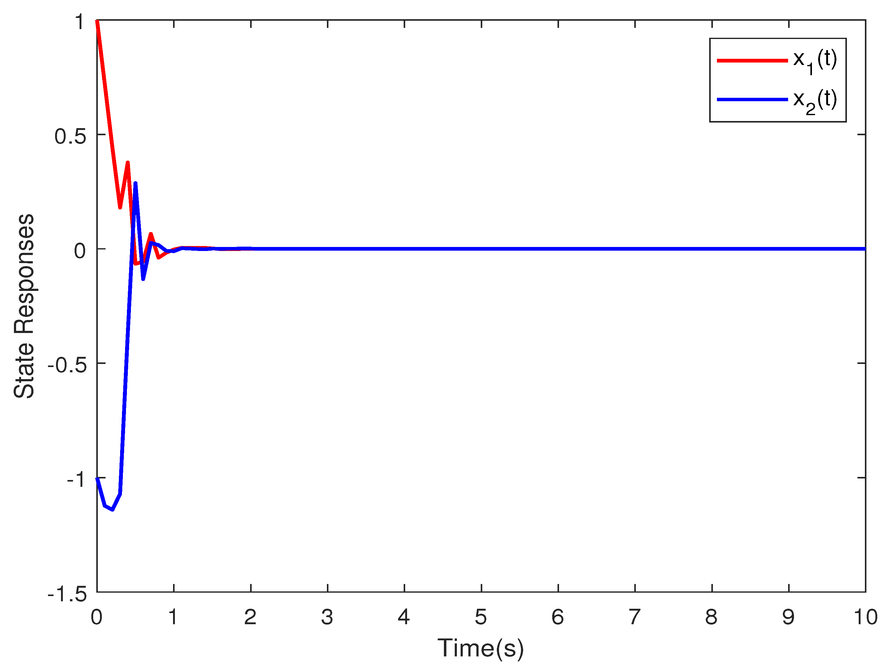
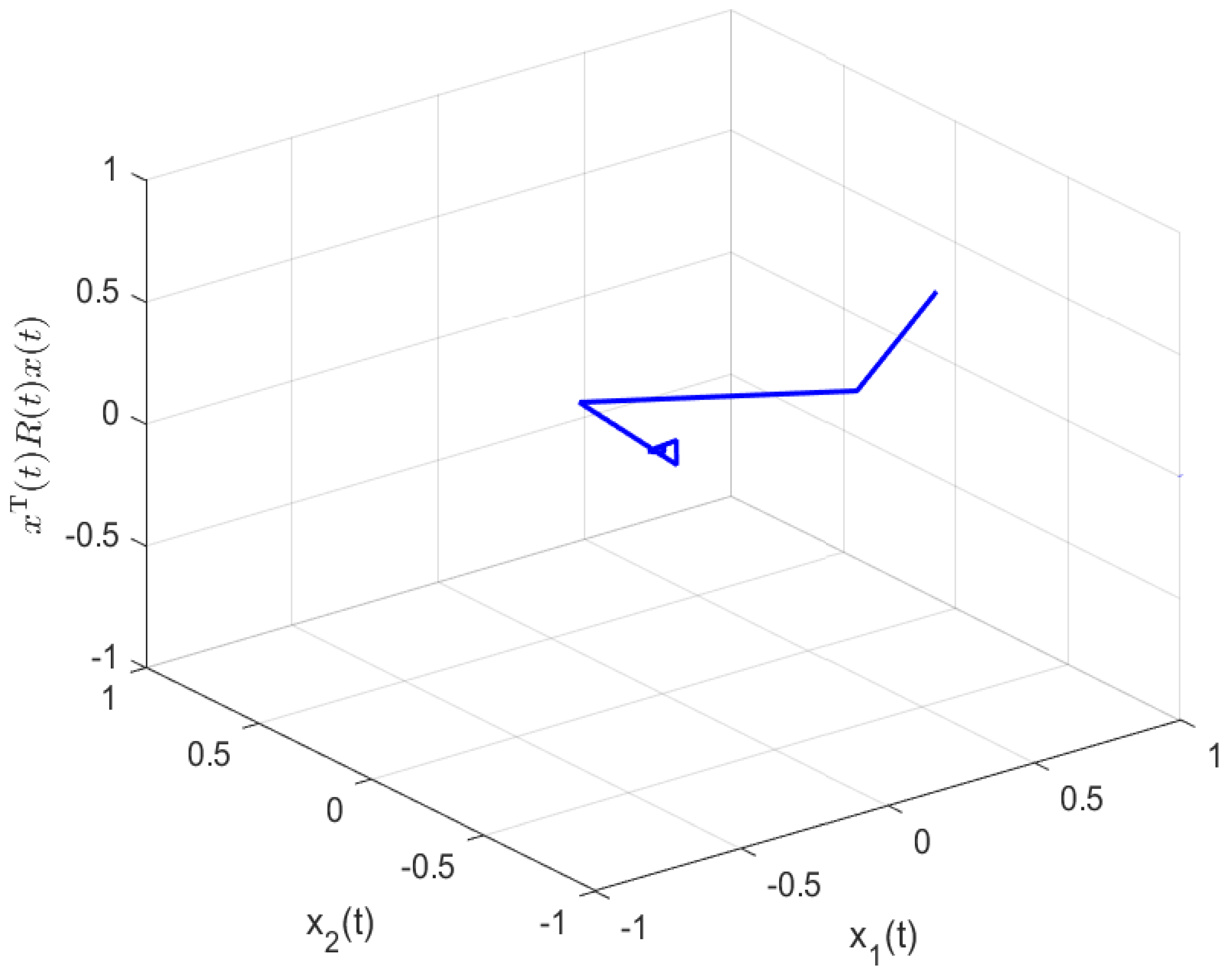
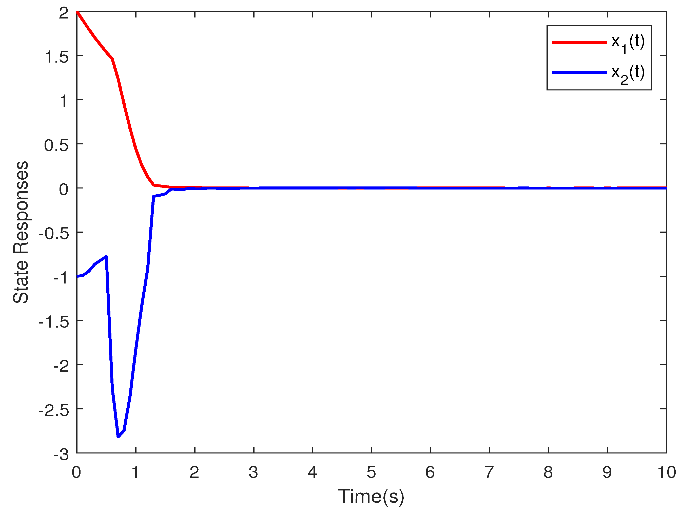
4. Illustrative Example

Example 1.

Consider a non-homogeneous hidden semi-Markov jump system with two subsystems:

$$\left[\begin{array}{c}{A}_1 | A_2\end{array}\right]=\left[\begin{array}{cccc}-1& 2& -2& -3\\ -3& -2& 4& -1\end{array}\right],$$

$$B_1=B_2=R=\left[\begin{array}{cc}1& 0\\ 0& 1\end{array}\right],$$

$$\left[\begin{array}{c}{C}_1 | C_2\end{array}\right]=\left[\begin{array}{cc}0.001& -0.001\\ -0.001& -0.001\end{array}\right],\left[\begin{array}{c}{D}_1 | D_2\end{array}\right]=\left[\begin{array}{cc}0.2& 0.2\\ 0.4& 0.1\end{array}\right],$$

The transition rate matrix ${\mathsf{\Pi }}^p\left(\delta \right)$ is described by

$${\mathsf{\Pi }}^1\left(\delta \right)=\left[\begin{array}{cc}-3{\left(\delta \right)}^2& 3{\left(\delta \right)}^2\\ 4{\left(\delta \right)}^3& -4{\left(\delta \right)}^3\end{array}\right],{\mathsf{\Pi }}^2\left(\delta \right)=\left[\begin{array}{cc}-4{\left(\delta \right)}^3& 4{\left(\delta \right)}^3\\ 3{\left(\delta \right)}^2& -3{\left(\delta \right)}^2\end{array}\right].$$

The semi-Markov chain dwell time for each mode is assumed to follow a Weibull distribution. ${\mathcal{F}}_i^p\left(\delta \right)$ refers to the probability density functions of DT with respect to δ, where $d{\mathcal{F}}_1^1\left(\delta \right)=3{\left(\delta \right)}^2{e}^{-{\left(\delta \right)}^3}d\delta$, $d{\mathcal{F}}_2^1\left(\delta \right)=4{\left(\delta \right)}^3{e}^{-{\left(\delta \right)}^4}d\delta$, $d{\mathcal{F}}_2^2\left(\delta \right)=3{\left(\delta \right)}^2{e}^{-{\left(\delta \right)}^3}d\delta$, and $d{\mathcal{F}}_1^2\left(\delta \right)=4{\left(\delta \right)}^3{e}^{-{\left(\delta \right)}^4}d\delta$. Further, the mathematical expectation can be calculated:

$$\begin{array}{c}\hfill {\left[{\overline{\pi }}_{ij}\right]}^1=\left[\begin{array}{cc}-2.7082& 2.7082\\ 3.6763& -3.6763\end{array}\right],{\left[{\overline{\pi }}_{ij}\right]}^2=\left[\begin{array}{cc}-3.6763& 3.6763\\ 2.7082& -2.7082\end{array}\right].\end{array}$$

Case I: Asynchronous case: we define the emission probability matrix.

$$\begin{array}{ccc}\hfill \left[{\rho }_{im}\right]& =& \left[\begin{array}{cc}0.5\hfill & 0.5\hfill \\ 0.2\hfill & 0.8\hfill \end{array}\right].\hfill \end{array}$$

By choosing $\alpha =1$, $\gamma =0.1$, $c_1=0.4$, $c_2=20$, $T=4$, $d=2$, $x_0={[1,-1]}^{\mathrm{T}}$, and $\omega \left(t\right)=e^{-2t}sin\left(0.5t\right)$ and solving Theorem 2, we obtain the three-variable-dependent asynchronous feedback control gain matrix:

$$\left[\begin{array}{cc}{K}_{111}& K_{121}\end{array}\right]=\left[\begin{array}{cccc}0.2312& 1.0238& 0.2216& 1.0135\\ -4.8556& -12.6636& -4.8641& -12.6847\end{array}\right],$$

$$\left[\begin{array}{cc}{K}_{211}& K_{221}\end{array}\right]=\left[\begin{array}{cccc}0.2227& 1.0148& 0.2323& 1.0252\\ -4.8704& -12.7001& -4.8619& -12.6791\end{array}\right],$$

$$\left[\begin{array}{cc}{K}_{112}& K_{122}\end{array}\right]=\left[\begin{array}{cccc}-2.4428& -1.1474& -2.4407& -1.1465\\ 1.1370& 1.1520& 1.1371& 1.1521\end{array}\right],$$

$$\left[\begin{array}{cc}{K}_{212}& K_{221}\end{array}\right]=\left[\begin{array}{cccc}-9.7750& -4.5913& -9.7755& -4.5916\\ 4.5435& 4.6040& 4.5435& 4.6040\end{array}\right].$$

The trajectories of the state response are shown in Figure 2. It can be clearly seen from Figure 3 that the evolution of $x^{\mathrm{T}}\left(t\right)Rx\left(t\right)$ tends to zero in finite time, and the designed asynchronous controllers can make non-homogeneous HSMJSs (5) become SFTB. Figure 4 and Figure 5 show the system mode and controller mode, which both have two modes. Figure 6 shows a possible evolution of the switching signal ${\theta }_t$.

Case II: Synchronous case: we define the emission probability matrix.

$$\begin{array}{ccc}\hfill \left[{\rho }_{im}\right]& =& \left[\begin{array}{cc}1.0\hfill & 0.0\hfill \\ 0.0\hfill & 1.0\hfill \end{array}\right].\hfill \end{array}$$

The other parameters are the same as in case I.

The trajectories of the state response are shown in Figure 7. It can be clearly seen from Figure 8 that the evolution of $x^{\mathrm{T}}\left(t\right)Rx\left(t\right)$ tends to zero in finite time, and the designed synchronous controllers can make non-homogeneous HSMJSs (5) become SFTB. These figures fully demonstrate the effectiveness of the method presented in this paper.

Remark 4.

From case I and case II, it can be seen that, differing from the existing literature [30,31], the method adopted in this paper can not only deal with the stochastic finite-time boundedness problem in the case of an asynchronous controller and system mode but also with the stochastic finite-time boundedness problem in the case of a synchronous controller and system mode, so the method in this paper has wider practicability and generality.

Example 2.

Next, we consider a single-link robot arm system from [28], which can be expressed as

$$\begin{array}{ccc}\hfill \ddot{\psi }\left(t\right)& =& -{\displaystyle \frac{M_{r_t}\mathrm{gL}}{J_{r_t}}}sin\left(\psi \left(t\right)\right)-{\displaystyle \frac{W}{J_{r_t}}}\dot{\psi }\left(t\right)+{\displaystyle \frac{1}{J_{r_t}}}u\left(t\right),\hfill \end{array}$$

in which $\psi \left(t\right)$, $\dot{\psi }\left(t\right)$, and $\ddot{\psi }\left(t\right)$ separately stand for the angle, angular velocity, and angular acceleration, $J_{r_t}$ represents the moment of inertia, $M_{r_t}$ and L are the total mass and the length of the arm, respectively, g denotes the gravitational acceleration, and W is the coefficient of viscous friction. The robot runs under different payloads that obey the SMP $\{r_t,t\ge 0\}$ in ${\mathcal{M}}_1$, and $\{{\sigma }_t,t\ge 0\}$ in ${\mathcal{M}}_2$ is the asynchronous controller mode. Define $x\left(t\right)={\left[x_1^{\mathrm{T}}\left(t\right)x_2^{\mathrm{T}}\left(t\right)\right]}^{\mathrm{T}}$, where $x_1\left(t\right)=\psi \left(t\right)$ and $x_2\left(t\right)=\dot{\psi }\left(t\right)$. Thus, when $r_t=i$, one has the linearized system

$$\begin{array}{ccc}\hfill \dot{x}\left(t\right)& =& \left[\begin{array}{cc}0& 1\\ -{\displaystyle \frac{M_i\mathrm{gL}}{J_i}}& -{\displaystyle \frac{W}{J_i}}\end{array}\right]x\left(t\right)+\left[\begin{array}{c}0\\ {\displaystyle \frac{1}{J_i}}\end{array}\right]u\left(t\right).\hfill \end{array}$$

For every single-link robot arm, let $J_1=0.15$, $J_2=0.25$, $M_1=0.5$, $M_2=1$, $L=0.5$, $W=2$, $g=9.81$, $x_0={[2,-1]}^{\mathrm{T}}$, and $\omega \left(t\right)=sin\left(t\right)$. The other parameters are the same as in Example 1 Case I. Solving Theorem 2, we obtain the three-variable-dependent asynchronous feedback control gain matrix:

$$\left[\begin{array}{cc}{K}_{111}& K_{121}\end{array}\right]=\left[\begin{array}{cccc}1.7565& 0.5955& 1.7306& 0.5424\end{array}\right],$$

$$\left[\begin{array}{cc}{K}_{211}& K_{221}\end{array}\right]=\left[\begin{array}{cccc}2.6850& 0.7930& 0.6636& 0.1921\end{array}\right],$$

$$\left[\begin{array}{cc}{K}_{112}& K_{122}\end{array}\right]=\left[\begin{array}{cccc}1.7636& 0.5599& 1.7808& 0.5968\end{array}\right],$$

$$\left[\begin{array}{cc}{K}_{212}& K_{221}\end{array}\right]=\left[\begin{array}{cccc}2.4764& 0.6709& 0.6141& 0.1638\end{array}\right].$$

The trajectories of the state response are shown in Figure 9. It can be clearly seen from Figure 10 that the evolution of $x^{\mathrm{T}}\left(t\right)Rx\left(t\right)$ tends to zero in finite time, and the designed asynchronous controllers can make non-homogeneous HSMJSs (5) become SFTB.

5. Conclusions

This article explores the finite-time control problem associated with a specific category of non-homogeneous hidden semi-Markov jump systems. A novel piecewise homogeneous strategy is presented to adequately address the challenges posed by the non-homogeneous nature of the system. Furthermore, based on Lyapunov theory, the closed-loop non-homogeneous HSMJSs can be stochastically finite-time-bounded and satisfy the $H_{\infty }$ performance. To demonstrate the practical applicability and effectiveness of the proposed method, two simulation examples were employed. The issue of cyber attacks targeting network control systems has emerged as a significant concern this year, prompting us to investigate it further in our upcoming research. This study will investigate the finite-time stability of non-homogeneous hidden semi-Markov jump systems within the context of complex cyber attack environments.

References

1. Wu, Z.; Shi, P.; Shu, Z.; Su, H.; Lu, R. Passivity-Based Asynchronous Control for Markov Jump Systems. IEEE Trans. Autom. Control 2017, 62, 2020–2025. [Google Scholar] [CrossRef]
2. Wang, Y.; Zhuang, G.; Chen, X.; Wang, Z.; Chen, F. Dynamic event-based finite-time mixed H and passive asynchronous filtering for T-S fuzzy singular Markov jump systems with general transition rates. Nonlinear Anal.-Hybrid Syst. 2020, 36, 100874. [Google Scholar] [CrossRef]
3. Cheng, J.; Wu, Y.; Yan, H.; Wu, Z.; Shi, K. Protocol-based filtering for fuzzy Markov affine systems with switching chain. Automatica 2022, 141, 110321. [Google Scholar] [CrossRef]
4. Wang, H.; Luan, X.; Stojanovic, V.; Liu, F. Self-triggered finite-time control for discrete-time Markov jump systems. Inf. Sci. 2023, 634, 101–121. [Google Scholar]
5. Shen, H.; Hu, X.; Wang, J.; Cao, J.; Qian, W. Non-Fragile H Synchronization for Markov Jump Singularly Perturbed Coupled Neural Networks Subject to Double-Layer Switching Regulation. IEEE Trans. Neural Netw. Learn. Syst. 2023, 34, 2682–2692. [Google Scholar] [CrossRef]
6. Li, F.; Wu, L.; Shi, P.; Lim, C. State estimation and sliding mode control for semi-Markovian jump systems with mismatched uncertainties. Automatica 2015, 51, 385–393. [Google Scholar] [CrossRef]
7. Shen, H.; Park, J.; Wu, Z.; Zhang, Z. Finite-time H synchronization for complex networks with semi-Markov jump topology. Commun. Nonlinear Sci. Numer. Simul. 2015, 24, 40–51. [Google Scholar] [CrossRef]
8. Wang, B.; Zhu, Q. Stability analysis of semi-Markov switched stochastic systems. Automatica 2018, 94, 72–80. [Google Scholar] [CrossRef]
9. Wang, J.; Hu, X.; Wei, Y.; Wang, Z. Sampled-data synchronization of semi-Markov jump complex dynamical networks subject to generalized dissipativity property. Appl. Math. Comput. 2019, 346, 853–864. [Google Scholar] [CrossRef]
10. Zhang, L.; Lam, H.; Liang, Y.S.H. Fault Detection for Fuzzy Semi-Markov Jump Systems Based on Interval Type-2 Fuzzy Approach. IEEE Trans. Fuzzy Syst. 2020, 28, 2375–2388. [Google Scholar] [CrossRef]
11. Yang, J.; Zhu, Y.; Zhang, L.; Duan, G. Smooth control with flexible duration for semi-Markov jump linear systems. Automatica 2024, 164, 111612. [Google Scholar] [CrossRef]
12. Wang, Q.; Zhang, X.; Zhang, R. Finite-time H control for continuous-time non-homogeneous semi-Markov jump systems. In Proceedings of the 2023 IEEE 11th International Conference on Information, Communication and Networks, Xi’an, China, 17–20 August 2023. [Google Scholar]
13. Kim, S. Stochastic stability and stabilization conditions of semi-Markovian jump systems with mode transition-dependent sojourn-time distributions. Inf. Sci. 2017, 385–386, 314–324. [Google Scholar] [CrossRef]
14. Nguyen, K.; Kim, S. Observer-based control design of semi-Markovian jump systems with uncertain probability intensities and mode-transition-dependent sojourn-time distribution. Appl. Math. Comput. 2020, 372, 124968. [Google Scholar] [CrossRef]
15. Cheng, J.; Xie, L.; Park, J.; Yan, H. Protocol-Based Output-Feedback Control for Semi-Markov Jump Systems. IEEE Trans. Autom. Control 2022, 67, 4346–4353. [Google Scholar] [CrossRef]
16. Wang, D.; Wu, F.; Lian, J.; Li, S. Observer-Based Asynchronous Control for Stochastic Nonhomogeneous Semi-Markov Jump Systems. IEEE Trans. Autom. Control 2024, 69, 2559–2566. [Google Scholar] [CrossRef]
17. Zhang, L.; Sun, Y.; Li, H.; Liang, H.; Wang, J. Event-triggered fault detection for nonlinear semi-Markov jump systems based on double asynchronous filtering approach. Automatica 2022, 138, 110144. [Google Scholar] [CrossRef]
18. Men, Y.; Sun, J. Asynchronous Control of 2-D Semi-Markov Jump Systems Under Actuator Saturation. IEEE Trans. Circuits Syst. II-Express Briefs 2023, 70, 4118–4122. [Google Scholar] [CrossRef]
19. Li, R.; Qi, W.; Park, J.; Cheng, J.; Shi, K. Sliding mode control for discrete interval type-2 fuzzy semi-Markov jump models with delay in controller mode switching. Fuzzy Sets Syst. 2024, 483, 108915. [Google Scholar] [CrossRef]
20. Liu, Y.; Wu, H.; Zhang, X. Stability and H performance of human-in-the-loop control systems through hidden semi-Markov human behavior modeling. Appl. Math. Model. 2023, 116, 799–815. [Google Scholar] [CrossRef]
21. Cai, B.; Zhang, L.; Shi, Y. Control Synthesis of Hidden Semi-Markov Uncertain Fuzzy Systems via Observations of Hidden Modes. IEEE Trans. Cybern. 2020, 50, 3709–3718. [Google Scholar] [CrossRef]
22. Men, Y.; Sun, J. H control of singularly perturbed systems using deficient hidden semi-Markov model. Nonlinear Anal.-Hybrid Syst. 2024, 52, 101453. [Google Scholar] [CrossRef]
23. Wu, E.; Zhu, L.; Li, G.; Li, H. Nonparametric Hierarchical Hidden Semi-Markov Model for Brain Fatigue Behavior Detection of Pilots during Flight. IEEE Trans. Intell. Transp. Syst. 2022, 23, 5245–5256. [Google Scholar] [CrossRef]
24. Li, F.; Zheng, W.; Xu, S. Stabilization of Discrete-Time Hidden Semi-Markov Jump Singularly Perturbed Systems with Partially Known Emission Probabilities. IEEE Trans. Autom. Control 2022, 67, 4234–4240. [Google Scholar] [CrossRef]
25. Zhang, L.; Cai, B.; Tan, T. Stabilization of non-homogeneous hidden semi-Markov Jump systems with limited sojourn-time information. Automatica 2020, 117, 108963. [Google Scholar] [CrossRef]
26. Shen, H.; Zhang, Z.; Li, F.; Yan, H. Non-Fragile H Control for Piecewise Homogeneous Hidden Semi-Markov Lur’e Systems. IEEE Trans. Circuits Syst. II-Express Briefs 2024, 71, 306–310. [Google Scholar] [CrossRef]
27. He, S.; Song, J.; Liu, F. Robust Finite-Time Bounded Controller Design of Time-Delay Conic Nonlinear Systems Using Sliding Mode Control Strategy. IEEE Trans. Syst. Man Cybern. 2018, 48, 1863–1873. [Google Scholar] [CrossRef]
28. Qi, W.; Zong, G.; Ahn, C. Input-Output Finite-Time Asynchronous SMC for Nonlinear Semi-Markov Switching Systems with Application. IEEE Trans. Syst. Man Cybern. 2022, 52, 5344–5353. [Google Scholar] [CrossRef]
29. Xia, Z.; He, S. Finite-time asynchronous H fault-tolerant control for nonlinear hidden markov jump systems with actuator and sensor faults. Appl. Math. Comput. 2022, 428, 127212. [Google Scholar] [CrossRef]
30. Wang, J.; Ru, T.; Xia, J. Finite-time synchronization for complex dynamic networks with semi-Markov switching topologies: An H event-triggered control scheme. Appl. Math. Comput. 2019, 356, 235–251. [Google Scholar] [CrossRef]
31. Zhong, S.; Zhang, W.; Li, K. Finite-time stability and asynchronous resilient control for Itô stochastic semi-Markovian jump systems. J. Frankl. Inst. 2022, 359, 1531–1557. [Google Scholar] [CrossRef]
Figure 1. An example of a hidden semi-Markov process.
Mathematics 12 03036 g001
Figure 2. State response of closed-loop system.
Mathematics 12 03036 g002
Figure 3. The evolution of x T ( t ) R x ( t ) .
Mathematics 12 03036 g003
Figure 4. The system mode r t .
Mathematics 12 03036 g004
Figure 5. The controller mode σ t .
Mathematics 12 03036 g005
Figure 6. Value of θ t .
Mathematics 12 03036 g006
Figure 7. State response of closed-loop system.
Mathematics 12 03036 g007
Figure 8. The evolution of x T ( t ) R x ( t ) .
Mathematics 12 03036 g008
Figure 9. State response of closed-loop system.
Mathematics 12 03036 g009
Figure 10. The evolution of x T ( t ) R x ( t ) .
Mathematics 12 03036 g010