Approximate Analytic Frequency of Strong Nonlinear Oscillator

Abstract

In this paper, a new analytic expression for the frequency of vibration of a strong nonlinear polynomial-type oscillator is introduced. The method for frequency calculation is based on the transformation of the nonlinear oscillators into linear ones using the equality of their amplitudes and periods of vibration. The frequency of the linear oscillator is assumed to be the sum of frequencies corresponding to each nonlinearity in the original oscillator separately, i.e., the sum of frequencies of truly nonlinear oscillators. The obtained frequency is a complex function of amplitude, coefficient and order of nonlinearity. For simplification, the frequencies of the truly nonlinear oscillators are modified as power order functions of the exact frequency of the cubic oscillator which is linearly dependent on the amplitude of vibration. In this paper, the approximate frequency expression is developed for the harmonic any-order nonlinear oscillator and oscillators with the sum of polynomial nonlinearities. The accuracy of the obtained frequencies is tested on the examples of non-integer order nonlinear oscillators and also on a quadratic-cubic oscillator. The difference between the analytical and exact, numerically obtained results is negligible. The suggested approximate frequency expression has a simple algebraic form and is suitable for application by engineers and technicians.

1. Introduction

There are a significant number of papers which consider the vibration properties of an oscillator with nonlinear elastic force, described as

$$\ddot{x}+{\omega }_0^{2}x+f\left(x\right)=0$$

(1)

where ${\omega }_0^2$ is the coefficient of the linear term and $f\left(x\right)$ is the nonlinear function of displacement x. Nowadays, there is no general analytic expression of the exact frequency and period of vibration of an oscillator (1).

A special type of oscillator which is most widely considered is the Duffing–harmonic one [1,2,3] with a linear and a cubic nonlinear term. The equation was treated numerically and with semi-numerical methods (for example, the wavelet-based computational algorithms method [4], the iteration method with the use of the Elzaki transform [5], the modified variational iteration method with Adomian method [6], the variational iteration method (VIM) associated with formable transformation [7], etc.) and semi-analytic methods [8]. To obtain the vibration property of (4), various analytic solving procedures are also developed, including harmonic and energy balance methods [9,10], various perturbation methods [11,12,13,14,15,16,17], the non-perturbative methodology [18], etc. Based on the obtained approximate results, it is seen that the frequency of vibration depends on the initial amplitude, and the frequency–amplitude relation for the Duffing oscillator is defined [19,20,21,22,23,24,25]. As for the special case of the Duffing oscillator, in papers [26,27,28], the truly cubic nonlinear oscillator is considered. It is obtained that the frequency of vibration depends directly on the linear amplitude. However, generalization of the model of oscillator was necessary and a truly nonlinear oscillator with integer or non-integer order was introduced. For the truly nonlinear oscillators, the closed form frequency–amplitude relation exists [29,30,31,32,33,34]. Unfortunately, the expression is very complex, and the computation is not familiar to most engineers and technicians. Namely, the analytical formula includes the special beta and gamma mathematical functions, which lead to trouble in practical vibration analysis.

To overcome this lack, the aim of this paper is to determine the approximate analytic formulation of the frequency and the period of vibration for the so-called ‘harmonic any-order nonlinear oscillator’ where

$$\ddot{x}+{\omega }_0^{2}x+c_1^{2}x{\left|x\right|}^{\alpha -1}=0$$

(2)

and also the formulation for the oscillator with a sum of nonlinearities of different orders

$$\ddot{x}+{\omega }_0^{2}x+{\sum }_{\alpha }{c}_{\alpha }^{2}x{\left|x\right|}^{\alpha -1}=0$$

(3)

where $\alpha \ge 1$, $\alpha \in \mathbb{R}$ is the order of nonlinearity, ${\omega }_0^2$ is the coefficient of the linear term, $c_{\alpha }^2$ is the coefficient of the nonlinear term.

This paper is divided into five sections. After the Introduction, in Section 2 the new approximate frequency of vibration for the truly nonlinear oscillator is introduced. Using the fact that the frequency of the truly cubic oscillator depends on the linear value of the initial amplitude, the approximate frequency of vibration for the integer and non-integer order truly nonlinear oscillator is developed. The outcome of the suggested method is a frequency–amplitude expression which is appropriate to calculate the approximate period of vibration of the truly nonlinear oscillators. This new expression represents a contribution of our research. In Section 3, the expression of the approximate frequency of the harmonic any-order nonlinear oscillator is developed. The frequency is a complex function of frequencies which correspond to a harmonic and a truly nonlinear oscillator with the integer or non-integer order. As an example, the frequency of a non-integer order nonlinear oscillator is computed. In Section 4, the generalized expression of the period of vibration for the oscillator with a sum of nonlinearities of the polynomial type is designed. As an example, an oscillator with linear, quadratic and cubic terms is considered. It is proved that the difference between the newly introduced frequency of the linear oscillator and the exact frequency, which corresponds to the nonlinear oscillator, is negligible. This paper ends with conclusions.

2. Exact and Approximate Frequency of the Truly Nonlinear Oscillator

For the truly nonlinear oscillator [32],

$$\ddot{x}+c_1^{2}x{\left|x\right|}^{\alpha -1}=0$$

(4)

with initial conditions

$$x\left(0\right)=A, \dot{x}\left(0\right)=0$$

(5)

and the exact period of vibration $T_{ex}$ is (see [32])

$$T_{ex}={\displaystyle \frac{4A^{\frac{1-\alpha }{2}}}{c_1\sqrt{2\left(\alpha +1\right)}}}B({\displaystyle \frac{1}{\alpha +1}},{\displaystyle \frac{1}{2}})$$

(6)

where B is the incomplete beta function [35], $\alpha$ is the order of nonlinearity, $c_1$ is the coefficient of nonlinearity and A is the amplitude of vibration. Using (6) and the relation [35],

$$B\left({\displaystyle \frac{1}{\alpha +1}},{\displaystyle \frac{1}{2}}\right)={\displaystyle \frac{\Gamma \left(\frac{1}{\alpha +1}\right)\Gamma \left(\frac{1}{2}\right)}{\Gamma \left(\frac{3+\alpha }{2\left(\alpha +1\right)}\right)}}$$

(7)

the exact frequency of vibration follows as

$${\omega }_{ex}={\displaystyle \frac{2\pi }{T_{ex}}}=c_1{A}^{{\displaystyle \frac{\alpha -1}{2}}}{c}_{ex}$$

(8)

with

$$c_{ex}=\sqrt{{\displaystyle \frac{(\alpha +1)\pi }{2}}}{\displaystyle \frac{\Gamma \left(\frac{3+\alpha }{2\left(\alpha +1\right)}\right)}{\Gamma \left(\frac{1}{\alpha +1}\right)}}$$

(9)

where $\Gamma \mathrm{i}\mathrm{s} \mathrm{t}\mathrm{h}\mathrm{e} \mathrm{g}\mathrm{a}\mathrm{m}\mathrm{m}\mathrm{a} \mathrm{f}\mathrm{u}\mathrm{n}\mathrm{c}\mathrm{t}\mathrm{i}\mathrm{o}\mathrm{n} \mathrm{a}\mathrm{n}\mathrm{d} \Gamma \left({\displaystyle \frac{1}{2}}\right)=\sqrt{\pi }$. Due to the complexity of the special function $\Gamma$, it is not an easy task to compute and analyze the coefficient $c_{ex}$. This is the reason that at this point the approximation of the frequency is introduced.

In papers [21,23], approximate frequencies for nonlinear oscillators with the integer order of nonlinearity (cubic and quantic) are introduced. Comparing these relations with (8), it is obvious that the expressions have the same form, but the difference is only in the value of the constant c. Thus, for example, according to He’s theory [20] for the nonlinear function $c_1^{2}x{\left|x\right|}^{\alpha -1}$, the approximate frequency relation follows as

$${\omega }_{He}=\sqrt{\alpha (x^{\alpha -1}{)}_{x={\displaystyle \frac{A}{2}}}}=c_1{A}^{{\displaystyle \frac{\alpha -1}{2}}}{c}_{He}$$

(10)

where

$$c_{He}={\displaystyle \frac{\sqrt{\alpha }}{2^{(\alpha -1)/2}}}$$

(11)

Comparing (8) and (9) with (10) and (11), for the truly cubic oscillator it is obtained that $c_{ex}=0.84721$ and $c_{He}={\displaystyle \frac{\sqrt{3}}{2}}=0.86602$, and the relative error of He’s approximate solution is 2.22%. The aim of this paper is to minimize the error by introducing a new type of approximate frequency.

The new approximate frequency, introduced in this paper, is based on the exact frequency (8) of the cubic oscillator, i.e., ${\omega =c}_{1}0.84721A$. Namely, the frequency of the cubic oscillator is the linear function of the initial amplitude A of vibration, while for $\alpha \ne 3$ the amplitude function of the frequency is of an integer or non-integer order. Comparing the frequencies of any-order truly nonlinear oscillator with a cubic oscillator, the approximate solution is assumed as

$${\omega }_{appr}=c_1(0.84721A{)}^{(\alpha -1)/2}$$

(12)

In

Table 1. Exact and approximate frequencies of truly nonlinear oscillators of various orders for $c_1=1$.

$\mathit{\alpha }$	${\mathit{\omega }}_{\mathit{e}\mathit{x}}$	${\mathit{\omega }}_{\mathit{H}\mathit{e}}$	$\frac{{\mathit{\omega }}_{\mathit{e}\mathit{x}}-{\mathit{\omega }}_{\mathit{H}\mathit{e}}}{{\mathit{\omega }}_{\mathit{e}\mathit{x}}}100\mathit{\%}$	${\mathit{\omega }}_{\mathit{a}\mathit{p}\mathit{p}\mathit{r}}$	$\frac{{\mathit{\omega }}_{\mathit{e}\mathit{x}}-{\mathit{\omega }}_{\mathit{a}\mathit{p}\mathit{p}\mathit{r}}}{{\mathit{\omega }}_{\mathit{e}\mathit{x}}}100\mathit{\%}$
3/2	$0.9545{0 A}^{1/4}$	$1.02988{ A}^{1/4}$	7.89	${0.95939A}^{1/4}$	0.51
2	$0.91468 A^{1/2}$	${1.00000 A}^{1/2}$	9.32	${0.92044 A}^{1/2}$	0.63
3	$0.84721 A$	$0.86602 A$	2.22	$0.84721 A$	0
4	$0.79240 A^{3/2}$	$0.70710 A^{3/2}$	10.7	${0.77984 A}^{3/2}$	1.58
5	$0.74683 A^2$	$0.55901 A^2$	25.1	$0.71776{ A}^2$	3.89

, the exact frequency (8), He’s frequency (10) and the new approximate frequency (12) for various orders of nonlinearity α and $c_1=1$ are presented. The relative error for the coefficients is also calculated.

From the data in Table 1, it is concluded that the suggested approximate frequency is closer to the exact one than to He’s frequency. The difference between the newly introduced approximate frequency and the exact frequency of vibration depends on the order of nonlinearity: the higher the order of nonlinearity, the higher the error. However, the accuracy of the approximate frequency is smaller than 4% for $\alpha <6 .$ In addition, Formula (10) is a simple algebraic expression suitable for application by technicians.

Using the data in Table 1, frequency–amplitude diagrams for $c_1=1$ and various values of α are plotted (see Figure 1): the ${\omega }_{ex}-A$ diagram corresponds to the exact frequency (6) and ${\omega }_{appr}-A$ to the approximate frequency (12). For all diagrams, it is common that the frequency increases with increases in the amplitude of vibration. For A < 1, the frequency decrease is faster, while for A > 1 the frequency increase is slower for higher orders of nonlinearity. The frequency–amplitude relation is linear for α=3. In addition, comparing the diagrams for the exact and the approximate values, it is obvious that the difference is more evident for α < 3 than for α > 3, specially if A > 1.

2.1. Transformation of the Truly Nonlinear Oscillator into the Linear One

The aim of the research is to transform the strong nonlinear oscillator (4) into a harmonic one. The transformation is based on the equality of amplitude and frequency, i.e., the period of vibration of the truly nonlinear oscillator and the linear one. Using the approximate frequency (12), the nonlinear oscillator (4) is transformed into a linear one

$$\ddot{x}+{\omega }_{appr}^{2}x=0$$

(13)

To compare the nonlinear and linear oscillator, x-t diagrams, obtained by solving (4) and (13), are plotted. Figure 2 shows diagrams for various orders of nonlinearity ($\alpha ={\displaystyle \frac{3}{2}}; 2; 3; 5).$ The initial conditions (5) are $A=1, \dot{x}\left(0\right)=0$ and the parameter is ${ c}_1^2$=1. From Figure 1, it is obvious that the amplitude and the period of vibration of the nonlinear oscillator and the corresponding transformed linear one are equal, but the shape of the response diagrams differs. For $\alpha ϵ\left[\mathrm{1,3}\right)$, the difference is almost negligible, while for $\alpha \ge 3$ it is significant. As the order of nonlinearity increases, the difference is higher but almost negligible.

Comparing the curves in Figure 2, it is also seen that for equal initial conditions, the periods of vibration for oscillators with various orders of nonlinearity are different. To obtain a certain constant period of vibration, the initial amplitude for each oscillator has to be computed. Thus, the period

$$T={\displaystyle \frac{2\pi }{c_1}}$$

(14)

can be realized with various truly nonlinear oscillators, where the amplitude of vibration satisfies the relation $(0.84721A{)}^{(\alpha -1)/2}$ = 1. In

Table 2. Initial amplitudes $A_S$ of the nonlinear oscillators having equal periods of vibration $T=2\pi /c_1$.

$\mathit{\alpha }$	1	3/2	2	3	4	5
AS	any	1.20429	1.19526	1.18034	1.16780	1.15714

, the amplitudes which satisfy (14) are presented.

From Table 2, it is obvious that for the constant period of vibration, the amplitude of vibration decreases with the increase in the order of nonlinearity. The transformation of the nonlinear oscillator into the linear one based on the equality of the period of vibration requires variation in the initial amplitude dependent on the order of nonlinearity. In Figure 3, x-t diagrams for nonlinear (4) and linear (13) oscillators, having equal periods of vibration (14), are plotted. The parameters are $c_1^2=1$, $\dot{x}\left(0\right)=0$ and there are various initial displacements $A$ dependent on the order of nonlinearity, given in Table 2.

Remark: Comparing the truly nonlinear oscillator (4) and the linear oscillator (13) for initial conditions (3), it is concluded that there exists a relation between the elastic forces $c_1^2{\left|x\right|}^{\alpha -1}x$ and ${\omega }^{2}x$ of the truly nonlinear and linear oscillators, i.e.,

$$F=c_1^2{\left|x\right|}^{\alpha -1}x\approx {\omega }^{2}x$$

(15)

In the model of the oscillator, the nonlinear elastic force $c_1^2{\left|x\right|}^{\alpha -1}x$ is substituted with the linear ${\omega }^{2}x$ one.

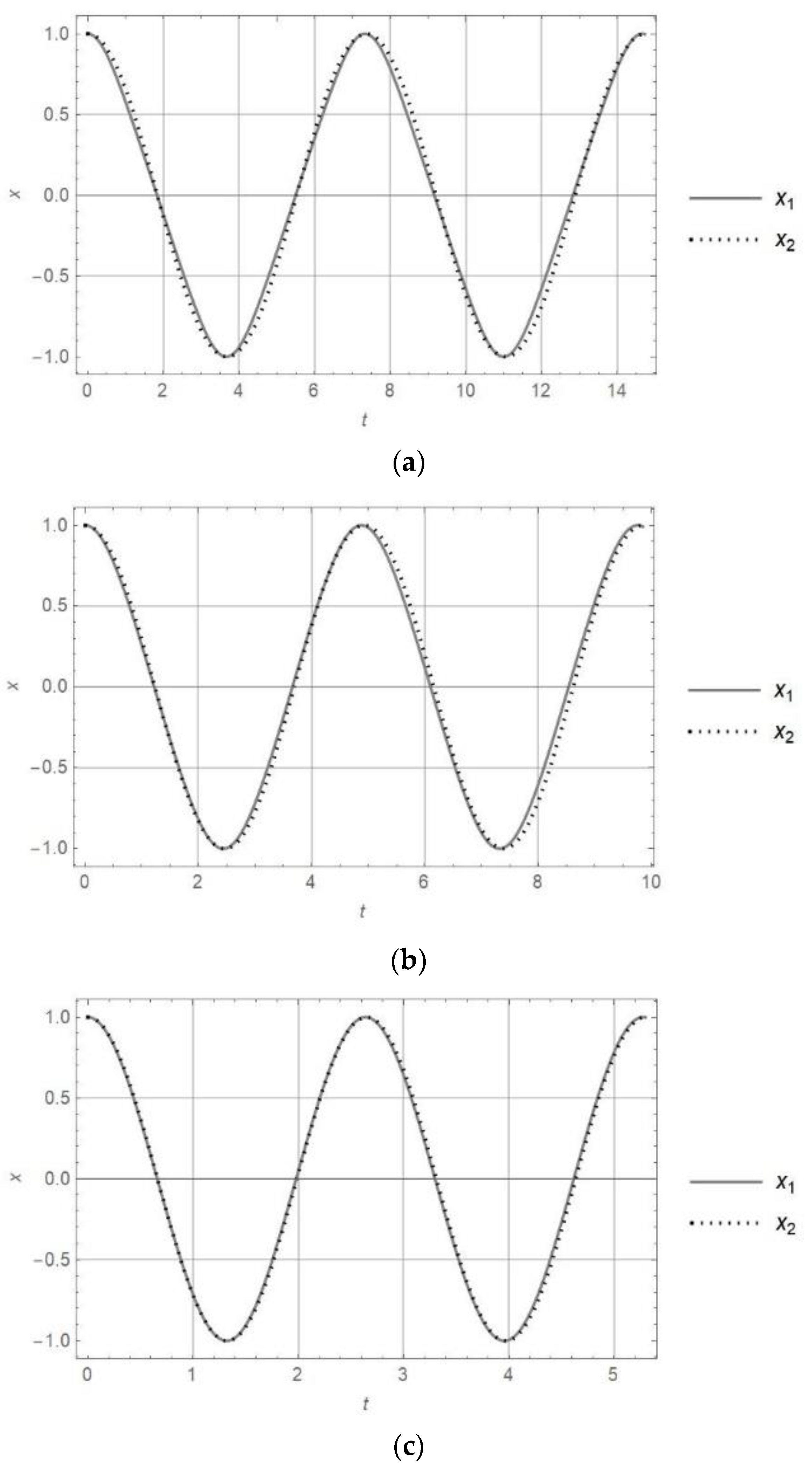
2.2. Example of a Truly Non-Integer Order Nonlinear Oscillator

The suggested method is applicable for computing the approximate frequency of any truly nonlinear integer or non-integer order oscillator. For example, the oscillator with an order of nonlinearity $\alpha =2.55$, i.e.,

$$\ddot{x}+c_1^{2}x{\left|x\right|}^{1.55}=0$$

(16)

has the approximate frequency (12)

$${\omega }_{appr}=c_1(0.84721 A{)}^{0.775}={0.87941c}_1{A}^{0.775}$$

(17)

and period of vibration

$$T_{appr}={\displaystyle \frac{2\pi }{{\omega }_{appr}}}={\displaystyle \frac{7.14433}{c_1{A}^{0.775}}}$$

(18)

Using the obtained data and transforming the nonlinear oscillator (16), the harmonic oscillator follows as

$$\ddot{x}+{(0.77336 c}_1^2{A}^{1.55})x=0$$

(19)

In Figure 4, the x-t responses of nonlinear Equation (16) and of the corresponding linear one (19) are plotted. The initial conditions are $x\left(0\right)=A=1$, $\dot{x}\left(0\right)=0$ and the coefficient of nonlinearity is $c_1=1.$

It is obtained that oscillators (16) and (19) have the same amplitude A of vibration and almost equal values of the period of vibration. According to (18), the approximate period of vibration is $T_{appr}=7.14433.$ Figure 4 shows that the difference between the exact and approximate period is negligible.

3. Approximate Frequency of Vibration of the Harmonic Any-Order Nonlinear Oscillator

Let us extend the elastic force (15) with the linear term ${\omega }_0^{2}x$. Then, the model of the harmonic any-order nonlinear oscillator follows as

$$\ddot{x}+{\omega }_0^2{x+c}_1^{2}x{\left|x\right|}^{\alpha -1}=0$$

(20)

Using the previous conclusion about the elastic force (15), let us introduce the assumption

$$F={\omega }_0^2{x+c}_1^{2}x{\left|x\right|}^{\alpha -1}\approx {\omega }_0^{2}x+{\omega }^{2}x$$

(21)

where $\omega$ is expressed with (8) or (12). According to (21) and the method of equivalent linearization based on the equality of amplitude and period of vibration, the nonlinear oscillator (20) is transformed into a linear one, i.e.,

$$\ddot{x}+{\omega }^{*2}x=0$$

(22)

where ${\omega }^{\mathrm{*}}=\sqrt{{\omega }_0^2+{\omega }^2}$, i.e., for (8)

$${\omega }^{*}=\sqrt{{\omega }_0^2+{c_1^2{A}^{\alpha -1}c}^2}$$

(23)

In (23) the principle of superposition, valid for the linear systems, is applied.

Unfortunately, the exact value of the period of vibration of the harmonic any-order nonlinear oscillator (20) (except for $\alpha =3$) is unknown. Because of that, in this section, the approximate period of vibration of the nonlinear oscillator (20) is assumed to be almost equal to that of the linear oscillator (22), i.e.,

$$T={\displaystyle \frac{2\pi }{\sqrt{{\omega }_0^2+{c_1^2{A}^{\alpha -1}c}^2}}}$$

(24)

To prove the accuracy of the period expression (24), it is computed for $\alpha =3$ and compared with the exact analytically obtained period of vibration for the Duffing equation

$$\ddot{x}+{\omega }_0^{2}x+c_1^{2}x{\left|x\right|}^2=0$$

(25)

For the initial conditions (5), the period of vibration (see [24]) is

$$T_{ex}={\displaystyle \frac{4K\left(k^2\right)}{\mathsf{\Omega }}}$$

(26)

where $K\left(k^2\right)$ is the Jacobi integral of the first order [36], and 4$K\left(k^2\right)$, $k^2$ and $\mathsf{\Omega }$ are the period, parameter and frequency of the cosine Jacobi elliptic function, respectively,

$$k^2={\displaystyle \frac{c_1^2{A}^2}{2({\omega }_0^2+c_1^2{A}^2)}}, {\mathsf{\Omega }}^2={\omega }_0^2+c_1^2{A}^2$$

(27)

The assumed period of vibration (24) for α = 3 is

$$T={\displaystyle \frac{2\pi }{{\omega }^{*}}}={\displaystyle \frac{2\pi }{\sqrt{{\omega }_0^2+2\pi {c_1^2{A}^2\left(\frac{\Gamma \left(\frac{3}{4}\right)}{\Gamma \left(\frac{1}{4}\right)}\right)}^2}}}={\displaystyle \frac{2\pi }{\sqrt{{\omega }_0^2+0.71705c_1^2{A}^2}}}$$

(28)

The result (26) with (27) is compared with (28) for the numerical values $A=1, c_1=1$ and ${\omega }_0^2$= 0; 0.1; 0.5; 1; 5; 10 (see

Table 3. Exact $T_{ex}$ and assumed T period of vibration for the Duffing oscillator for $c_1=1$, $A=1$ and various ${\omega }_0^2$.

${\mathit{\omega }}_0^2$	0	0.1	0.5	1	5	10
Tex (34)	7.41628	6.93312	5.66276	4.78227	2.6188	1.91641
T (36)	7.41628	6.93459	5.66872	4.78957	2.61931	1.91826
$\left|{\displaystyle \frac{T-T_{ex}}{T_{ex}}}\right|100 (\%)$	0	0.06540	0.09634	0.09448	0.08693	0.09678

). The difference between solutions (26) and (28) is computed by using the relative error.

Analyzing the data in Table 3, it is seen that the results $T$ and $T_{ex}$ are equal and the difference is only the consequence of the computation error in the special functions used.

3.1. Approximate Frequency Based on the Approximate Frequency of the Truly Nonlinear Oscillator

Substituting expression (12) into (21), the approximate frequency ${\omega }_{appr}^{*}$ and period $T_{appr}$ of the harmonic any-order nonlinear oscillator follow as

$${\omega }_{appr}^{*}=\sqrt{{\omega }_0^2+c_1^2(0.84721A{)}^{(\alpha -1)}}, T_{appr}={\displaystyle \frac{2\pi }{\sqrt{{\omega }_0^2+c_1^2{(0.84721 A)}^{\alpha -1}}}}$$

(29)

The accuracy of expression (29) has to be tested for any order of nonlinearity of oscillator (20). For this reason, the numerically obtained (exact) period of vibration of (20) is compared with the analytically suggested one (see (29)). In Figure 5 and Figure 6, the x-t diagrams obtained by solving (20) and (22) for α = 2 and α = 4, ${\omega }_0^2=0.1$; 1 and 5, $c_1^2=1$ and initial conditions $A=1, \dot{x}\left(0\right)=0$ are plotted. It is obtained that the analytically obtained period of vibration agrees with that obtained numerically. In addition, for the lower orders of nonlinearity (α < 3) and higher values of the linear term, the analytic and numeric x-t responses are close to each other, while for the higher orders of nonlinearity ($\alpha \ge 3$) and smaller ${\omega }_0^2$, the difference is more evident.

In

Table 4. Period of vibration $T_{appr}$ (29) of oscillator (22) for $c_1=1$, $A=1$ and various α and ${\omega }_0^2$.

${\mathit{\omega }}_0^2$	0	0.1	0.5	1	5	10
$\alpha =1$	6.28320	5.98774	5.12760	4.44063	2.56380	1.89349
$\alpha =3/2$	6.57874	6.24500	5.28639	4.54257	2.582976	1.90118
$\alpha =2$	6.86579	6.48893	5.43191	4.63391	2.59943	1.90771
$\alpha =4$	7.92930	7.36451	5.91625	4.92450	2.64853	1.92731
$\alpha =5$	8.40887	7.74333	6.10616	5.03165	2.66385	1.93274

, the periods of vibration (29) for various orders of nonlinearity α and coefficient ${\omega }_0^2$ are presented. The coefficient of nonlinearity is $c_1=1$ and the initial amplitude is $A=1.$ It is obtained that for α = const., the period of vibration decreases by increasing ${\omega }_0^2$.

The data in Table 4 show that for the same value of ${\omega }_0^2$, the period of vibration is higher for higher orders of nonlinearity α. However, the period of vibration variation is negligible when ${\omega }_0^2>10{\omega }^2$.

Analyzing the approximate frequency and period of vibration (29), it is obtained that for certain values of α and the constant ${\omega }_0^2$, the period of vibration decreases due to the increase in the initial amplitude and the nonlinear coefficient c₁. In

Table 5. Period of vibration $T_{appr}$ (29) for c₁ = 1, ${\omega }_0^2=1$, and various values of A and $\alpha$.

A	$\mathit{\alpha }=3/2$	$\mathit{\alpha }=2$	$\mathit{\alpha }=3$	$\mathit{\alpha }=4$	$\mathit{\alpha }=5$
0	6.28320	6.28320	6.28320	6.28320	6.28320
0.1	5.53318	6.03271	6.25758	6.27803	6.27825
0.5	4.89737	5.43191	5.78258	6.04717	6.17332
1	4.54257	4.63391	4.79158	4.92205	5.03165
AS (Table 2)	4.4429 (AS = 1.2043)	4.4429 (AS = 1.1953)	4.4429 (AS = 1.1803)	4.4429 (AS = 1.1678)	4.4429 (AS = 1.1571)
2	4.15113	3.84094	3.19187	2.55886	1.74517
3	3.60325	2.75842	1.33345	0.62784	0.33587

, for various initial amplitudes $A$ and orders of nonlinearity α (3/2; 2; 3; 4; 5) and ${\omega }_0^2=1$ and c₁ = 1, the approximate periods of vibration are computed. Analyzing the data in Table 5, it is seen that the period of vibration decreases by increasing the amplitude of vibration when the order of nonlinearity is a constant value. For oscillators with different orders of nonlinearity but the same initial amplitude A, which is smaller than the boundary amplitude $A_S$, the period of vibration increases with the order of nonlinearity, while it decreases with the increase in $\alpha$ for ${A>A}_S$. (For the boundary amplitude $A_S$, given in Table 2, the period of vibration for all oscillators is equal to a constant value T).

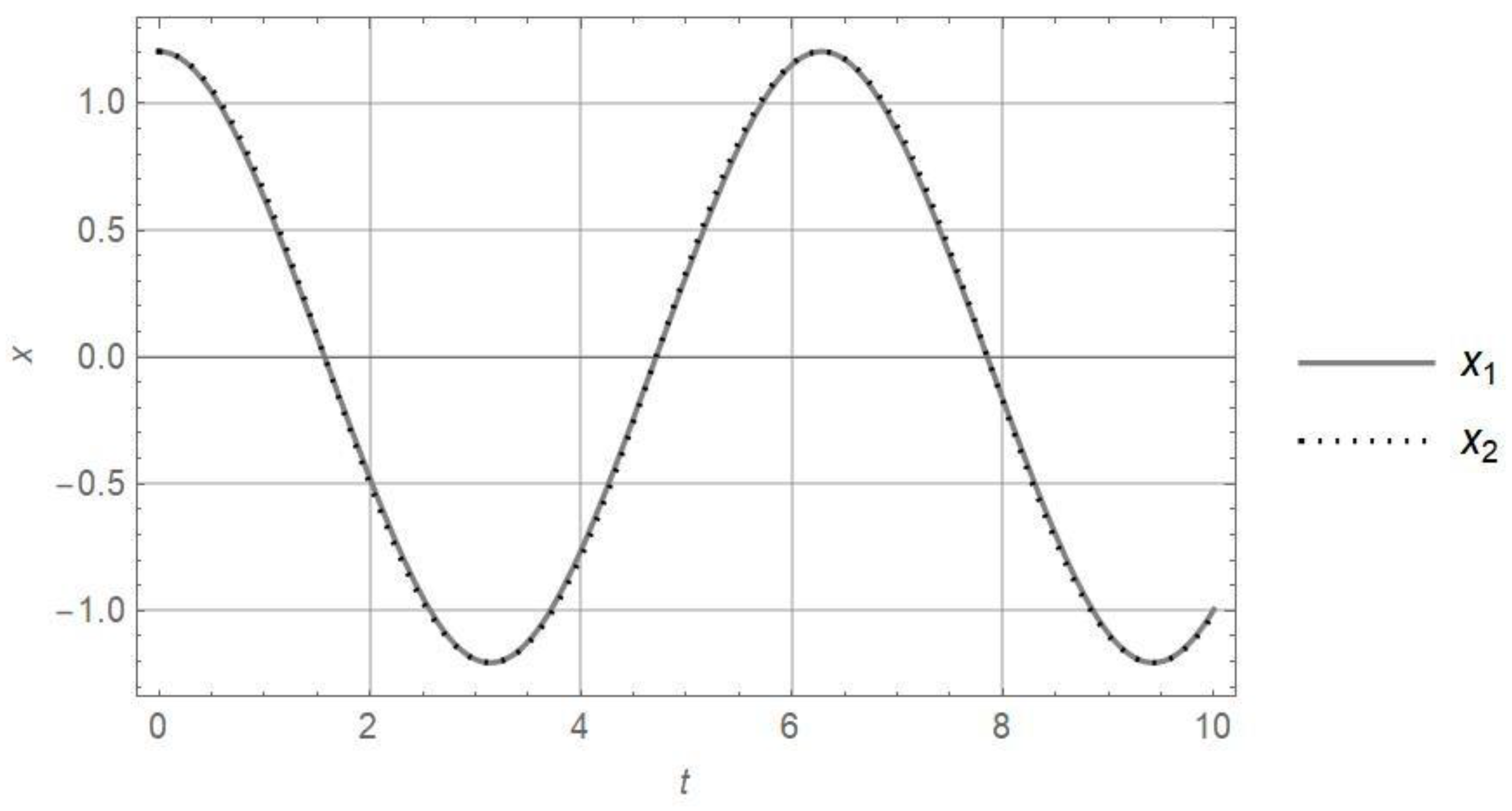
3.2. Example of a Harmoni–Non-Integer Order Nonlinear Oscillator

A model of an oscillator with a non-integer order of nonlinearity $\alpha =2.55$ is

$$\ddot{x}+{\omega }_0^{2}x+c_1^{2}x{\left|x\right|}^{1.55}=0$$

(30)

Using the expression for the approximate period of vibration (29)

$$T_{appr}={\displaystyle \frac{2\pi }{\sqrt{{\omega }_0^2+c_1^2{(0.84721 A)}^{1.55}}}}$$

(31)

the equivalent linear oscillator is

$$\ddot{x}+{(\omega }_0^2+c_1^2{(0.84721 A)}^{1.55})x=0$$

(32)

In Figure 7, an x-t diagram obtained by solving the nonlinear oscillator (30) (full line) and the linear oscillator (32) (dotted line) is plotted. The initial conditions are $x\left(0\right)=A=1$, $\dot{x}\left(0\right)=0$ and the coefficients are ${\omega }_0^2=1$ and $c_1=1.$

From Figure 7, it is obvious that the equivalent transformation from the nonlinear oscillator into the linear one has a high accuracy. In addition, the period of vibration calculated according to (31) is $T_{appr}=4.71585$, which corresponds to the period of vibration of the nonlinear oscillator (30).

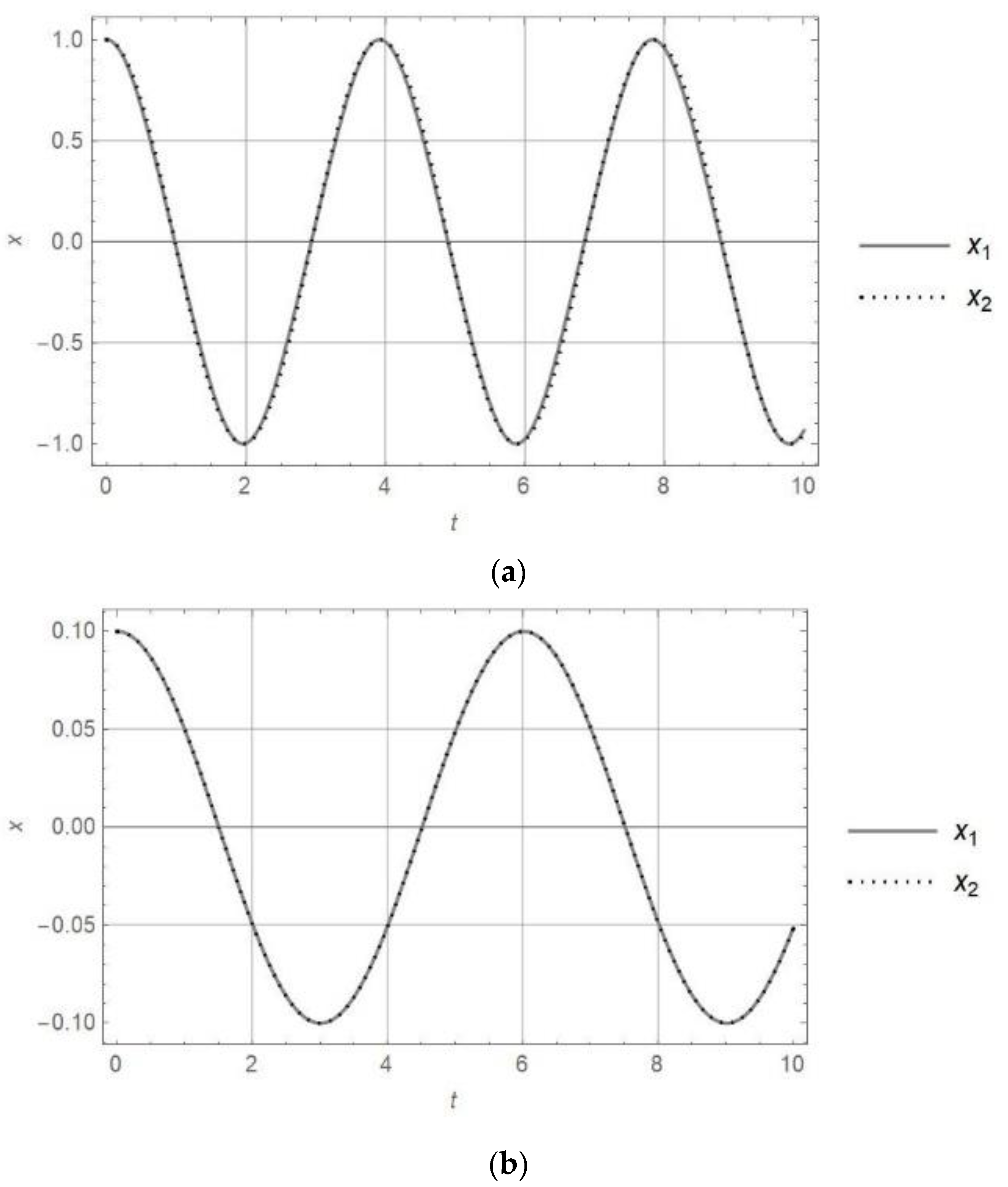
4. Frequency and Period of Oscillator with Sum of Nonlinearities of the Polynomial Type

For generalization, the oscillator which, in addition to the linear term, has a sum of various nonlinear terms, is considered. The model of the oscillator is

$$\ddot{x}+{\omega }_0^{2}x+{\sum }_{\alpha }{c}_{\alpha }^{2}x{\left|x\right|}^{\alpha -1}=0$$

(33)

where $c_{\alpha }$ is the coefficient of the nonlinear term of order α. According to the previous consideration and transformation of the nonlinear oscillator into the linear one, in this paper the approximate frequency of (34) is assumed to be the sum of frequencies ${\omega }_0$ of the linear oscillators and ${\omega }_{\alpha }$ of truly nonlinear oscillators of order $\alpha$, i.e.,

$${\omega }^{*2}={\omega }_0^2+{\sum }_{\alpha }{\omega }_{\alpha }^2$$

(34)

For the case when the exact frequencies (8) of the truly nonlinear oscillators are applied, the approximate frequency of (33) is

$${\omega }^{*2}={\omega }_0^2+{\sum }_{\alpha }{c}_{1\alpha }^2{A}^{\alpha -1}{c}_{\alpha }^2$$

(35)

where $c_{1\alpha }$ is the coefficient of nonlinearity and $c_{\alpha }$ corresponds to (9). For the approximate frequencies of truly nonlinear oscillators (12), the approximate frequency of (33) is assumed as

$${\omega }_{appr}^{*2}={\omega }_0^2+{\sum }_{\alpha }{c}_{1\alpha }^2({0.84721A)}^{\alpha -1}$$

(36)

and the approximate period of vibration

$$T_{appr}={\displaystyle \frac{2\pi }{\sqrt{{\omega }_0^2+{\sum }_{\alpha }{c}_{1\alpha }^2({0.84721A)}^{\alpha -1}}}}$$

(37)

The period of vibration depends on each of the coefficients in (33) but also on the order of nonlinearity and initial amplitude. Due to its simplicity, expression (37) is easily applied to calculate the period in any nonlinear oscillatory system. However, to prove the accuracy of the expression, two examples are calculated.

Example: Oscillator with Linear, Quadratic and Cubic Terms

Let us consider an oscillator with linear, quadratic and cubic terms modelled as

$$\ddot{x}+x+x\left|x\right|+x^3=0$$

(38)

After transformation of (38) for initial conditions (5), the equivalent linear oscillator with approximate frequency (36) follows.

$$\ddot{x}+x(1+0.84721A+0.71705A^2)=0$$

(39)

To compare oscillators (38) and (39), x-t diagrams for A = 1 (Figure 8a) and for A = 0.1 (Figure 8b) are plotted.

It is obtained that the approximate periods of vibrations $T_{appr}$= 3.92174 for A = 1 and $T_{appr}$= 6.02977 for A = 0.1 agree with the numerical values given in Figure 8a,b.

5. Conclusions

In this paper, the approximate frequency of a nonlinear oscillator is developed. The advantages and disadvantages of the expression are discussed and the following are concluded:

• The method of transformation of the oscillator with a strong polynomial nonlinearity of integer or non-integer orders into a linear oscillator, based on the equality or almost equality of periods of vibration, gives a result which is suitable for practical application in technics.
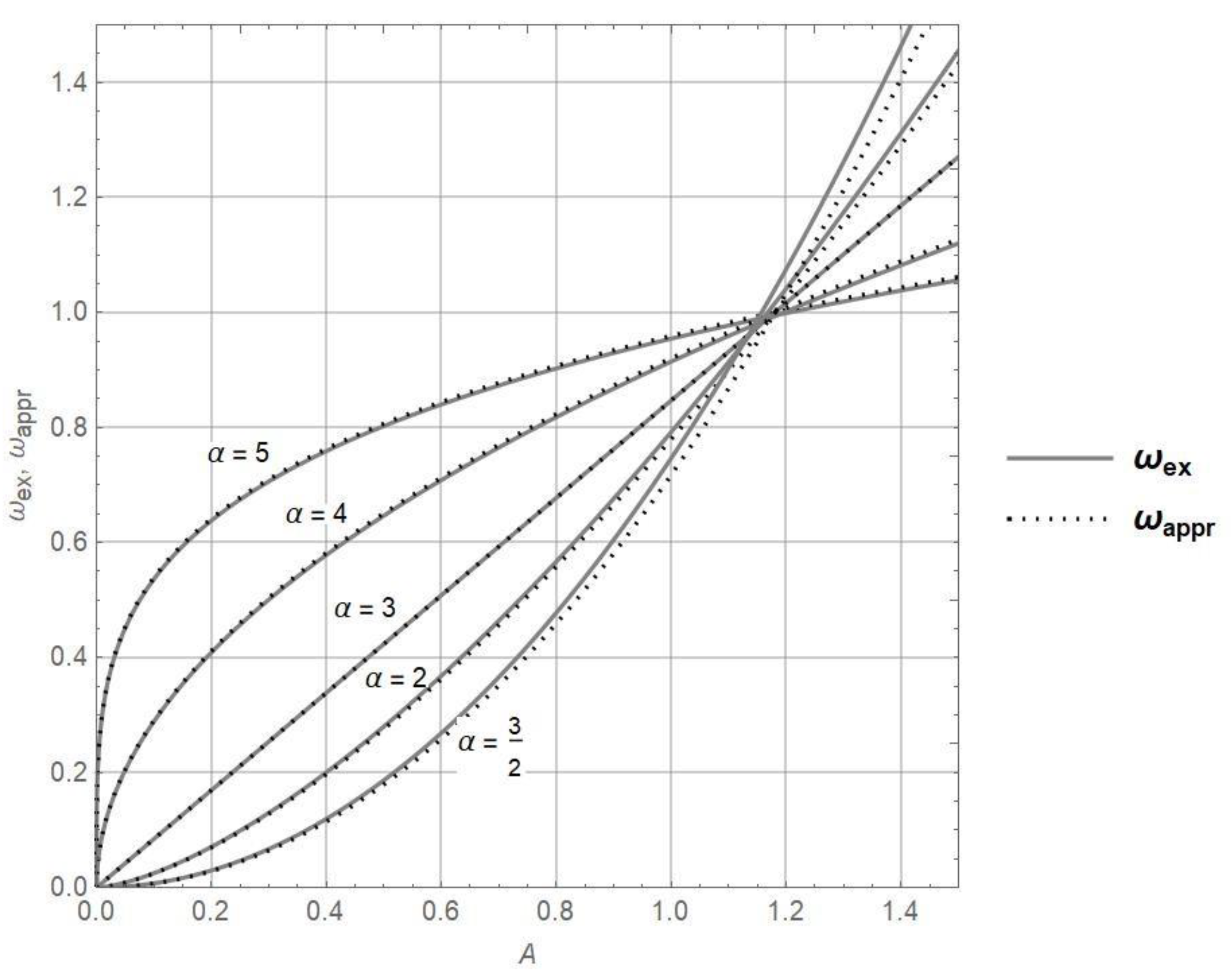
• The frequency of vibration of the truly strong nonlinear oscillator is approximately equivalent to $c_1^2$ ($0.84721{A)}^{(\alpha -1)}$, where c₁ is the coefficient of nonlinearity, A is the amplitude of vibration and $\alpha$ is the order of nonlinearity. The error of the approximate frequency is up to 4% in comparison to the exact one. The difference between the exact and suggested frequency is higher if the order of nonlinearity is lower and the amplitude of vibration is higher than one. Otherwise, the difference is negligible for higher orders of nonlinearity and amplitudes smaller than one.
• The recently developed approximate frequency of the harmonic any-order oscillator is the function of frequencies of the harmonic and the truly nonlinear oscillator. The test of the approximate expression for cubic nonlinearity shows good agreement with the exact frequency for the Duffing oscillator. For other orders of nonlinearity, the difference between approximate and exact periods of vibration of the nonlinear oscillator depends on the relation between the linear and nonlinear terms. However, when the linear term is 10 or more times higher than the nonlinear one, the period of vibration is negligible.
• The advantage of the suggested frequency expression is that it is useful for frequency computation for any non-integer order nonlinear oscillator. The analytic formulation is of the algebraic type and suitable for application by engineers and technicians.
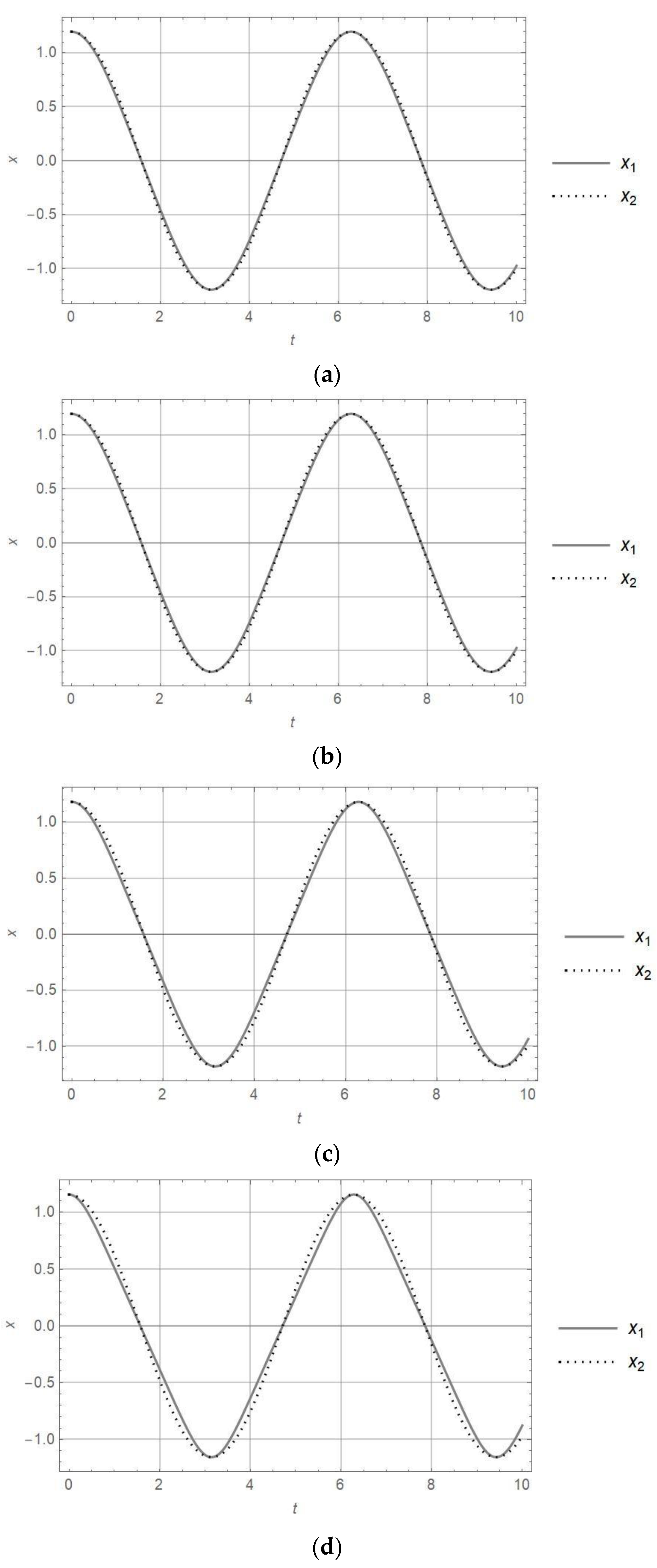
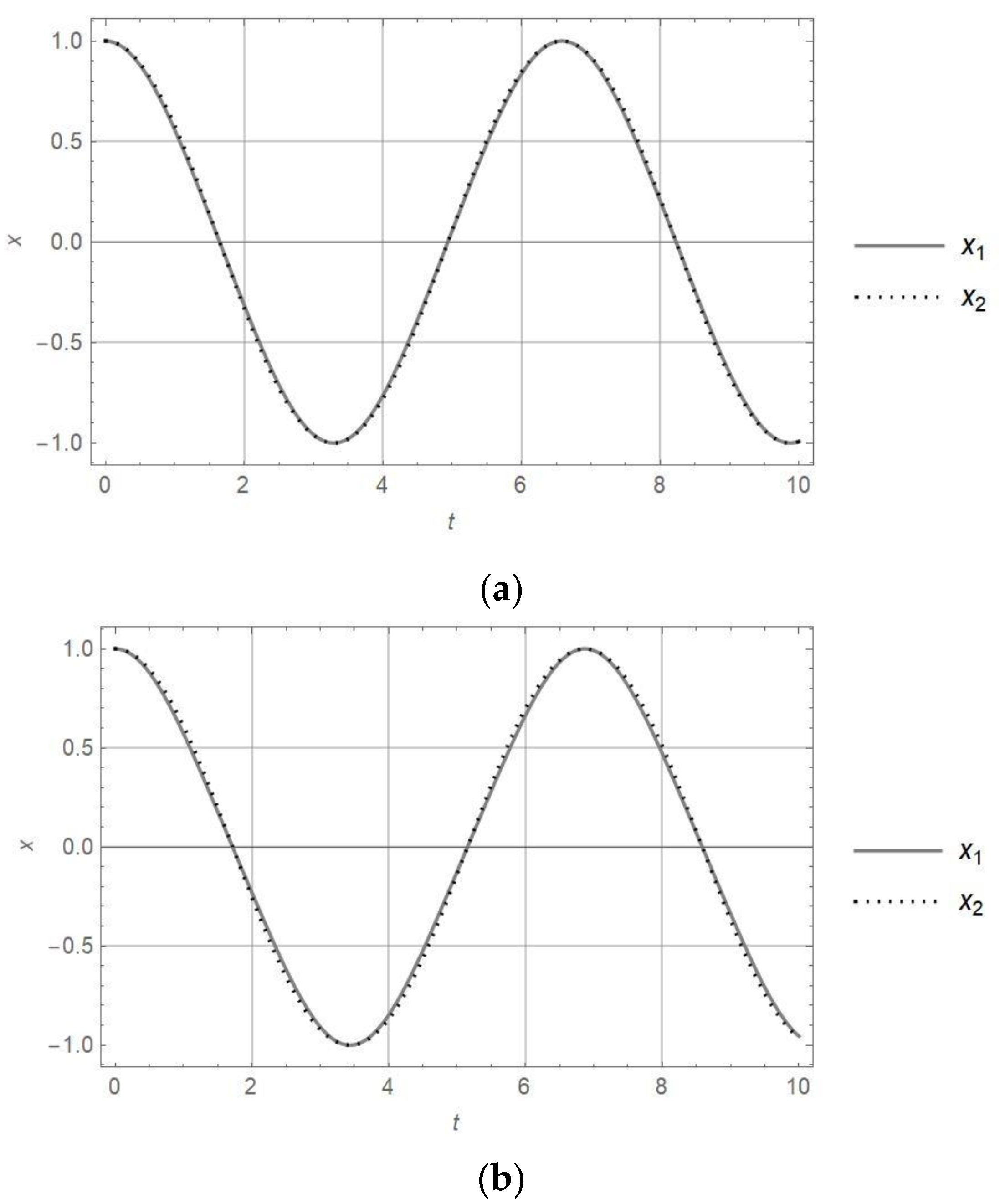
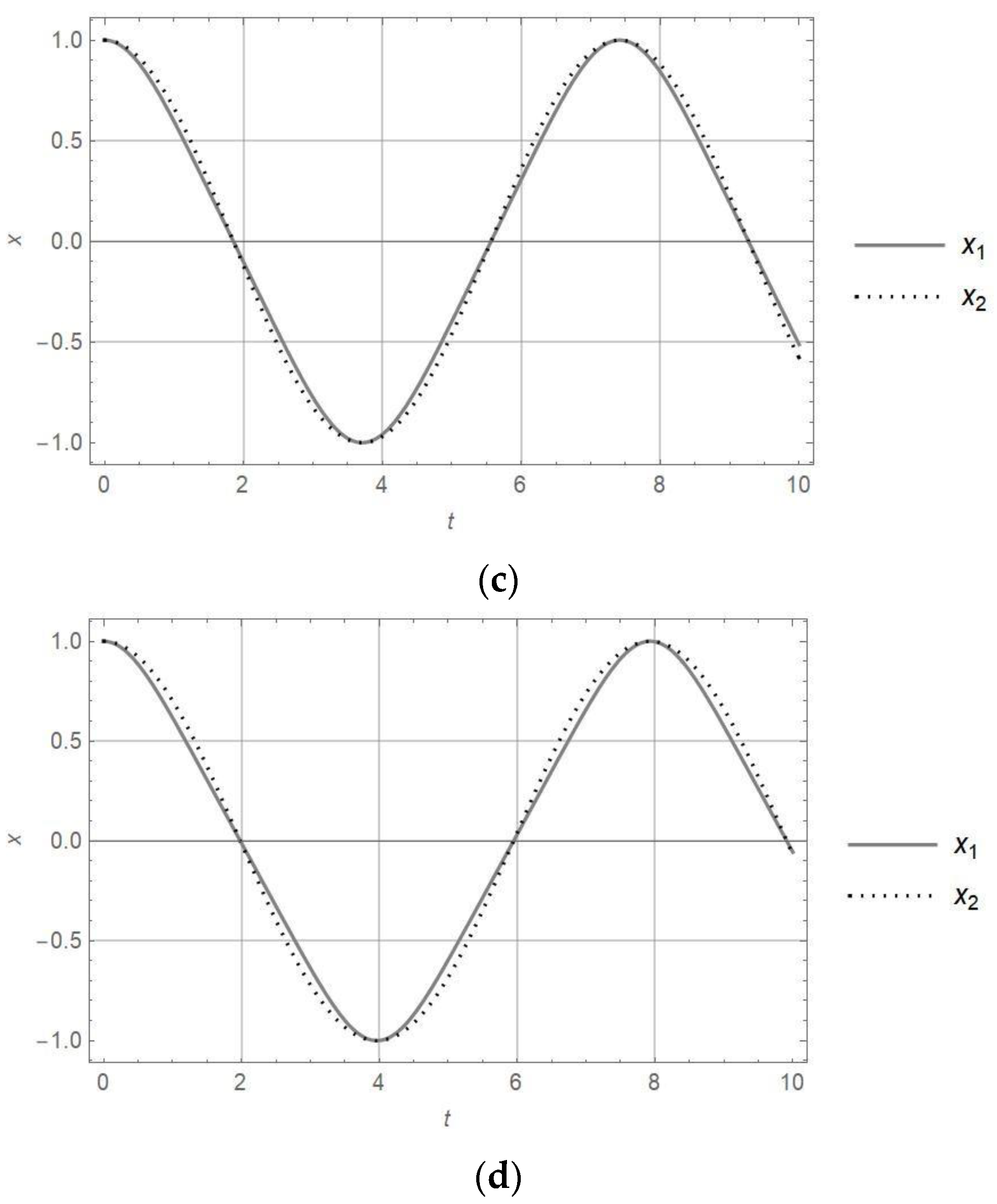
• The equivalent transformation of the nonlinear oscillator into the linear one, based on the equality of the period of vibration, shows that the responses for these oscillators are almost of the same form. It is valid for orders of nonlinearity up to four.
• Finally, in this paper it is suggested to apply the approximate linear oscillator obtained with equivalent transformation instead of the original complex nonlinear oscillator. The quantitative difference in the response and period of vibration is smaller than 5%, while the amplitude of vibration is equal.

Finally, future research could focus on the extension and modification of the suggested frequency formulation and also on developing a method to transform damped and forced nonlinear oscillators (for example, [37,38]) into equivalent linear ones.

References

1. Bogolubov, N.N.; Mitropolskij, Y.A. Asymptotic Methods in the Theory of Non-Linear Vibrations; Nauka: Moscow, Russian, 1968. (In Russian) [Google Scholar]
2. Nayfeh, A.H.; Mook, D.T. Nonlinear Oscillations; Wiley: New York, NY, USA, 1979. [Google Scholar]
3. Duffing, G. Erzwungene Schwingungen bei Veranderlicher Eigenfrequenz und ihre Technische Bedeutung; Vieweg & Sohn: Braunschweig, Germany, 1918. [Google Scholar]
4. Sathyaseelan, D.; Hariharan, G. Wavelet-based approximation algorithms for some nonlinear oscillator equations arising in engineering. J. Inst. Eng. Ser. C 2020, 101, 185–192. [Google Scholar] [CrossRef]
5. Anjum, N.; Suleman, M.; Lu, D.; He, J.H.; Ramzan, M. Numerical iteration for nonlinear oscillators by Elzaki transform. J. Low Freq. Noise Vib. Act. Control. 2020, 39, 879–884. [Google Scholar] [CrossRef]
6. He, W.; Kong, H.; Qin, Y.M. Modified variational iteration method for analytical solutions of nonlinear oscillators. J. Low Freq. Noise Vib. Act. Control. 2019, 38, 1178–1183. [Google Scholar] [CrossRef]
7. Tahir, M.; Shah, N.A.; Tag, S.M.; Imran, M. An application to formable transform: Novel numerical approach to study the nonlinear oscillator. J. Low Freq. Noise Vib. Act. Control. 2024, 43, 729–743. [Google Scholar]
8. Gamal, M.I.; Alwaleed, K.; Abdulaziz, A. Approximate analytical solutions to nonlinear oscillations via semi-analytical method. Alex. Eng. J. 2024, 98, 97–102. [Google Scholar]
9. Yeasmin, I.A.; Sharif, N.; Rahman, M.S.; Alam, M.S. Analytical technique for solving the quadratic nonlinear oscillator. Results Phys. 2020, 18, 103303. [Google Scholar] [CrossRef]
10. Sierra-Porta, D. Analytic approximations to Liénard nonlinear oscillators with modified energy balance method. J. Vib. Eng. Technol. 2020, 8, 713–720. [Google Scholar] [CrossRef]
11. Yu, D.N.; He, J.H.; Garcıa, A.G. Homotopy perturbation method with an auxiliary parameter for nonlinear oscillators. J. Low Freq. Noise Vib. Act. Control. 2019, 38, 1540–1554. [Google Scholar] [CrossRef]
12. Pasha, S.A.; Nawaz, Y.; Arif, M.S. The modified homotopy perturbation method with an auxiliary term for the nonlinear oscillator with discontinuity. J. Low Freq. Noise Vib. Act. Control. 2019, 38, 1363–1373. [Google Scholar] [CrossRef]
13. Manimegalai, K.; Zephania CF, S.; Bera, P.K.; Bera, P.; Das, S.K.; Sil, T. Study of strongly nonlinear oscillators using the Aboodh transform and the homotopy perturbation method. Eur. Phys. J. Plus 2019, 134, 264. [Google Scholar] [CrossRef]
14. Lashkarboluki, A.; Hosseini, H.; Ganji, D.D. Investigating the solutions of two classical nonlinear oscillators by the AG method. Int. J. Appl. Comput. Math. 2021, 7, 1–16. [Google Scholar] [CrossRef]
15. Ismail, G.M.; Mahmoud, A.E.; Mohra, Z.; Hijaz, A.; Maha, E.M. Highly accurate analytical solution for free vibrations of strongly nonlinear Duffing oscillator. J. Low Freq. Noise Vib. Act. Control. 2022, 41, 223–229. [Google Scholar] [CrossRef]
16. Song, P.; Shao, L.; Zhang, W. Residue-regulating homotopy method for strongly nonlinear oscillators. Nonlinear Dyn. 2022, 109, 1905–1921. [Google Scholar] [CrossRef]
17. Ismail, G.M.; El-Moshneb, M.M.; Zayed, M. A modified global error minimization method for solving nonlinear Duffing-harmonic oscillators. AIMS Math. 2023, 8, 484–500. [Google Scholar] [CrossRef]
18. Moatimid, G.M.; Amer, T.S.; Galal, A.A. Studying highly nonlinear oscillators using the non-perturbative methodology. Sci. Rep. 2023, 13, 20288. [Google Scholar] [CrossRef]
19. Kovacic, I.; Brennan, J.M. (Eds.) The Duffing Equation—Nonlinear Oscillators and Their Behaviour; Wiley: Chichester, UK, 2011. [Google Scholar]
20. He, J.H. The simplest approach to nonlinear oscillators. Results Phys. 2019, 15, 102546. [Google Scholar] [CrossRef]
21. He, J.H. The simpler, the better: Analytical methods for nonlinear oscillators and fractional oscillators. J. Low Freq. Noise Vib. Act. Control. 2019, 38, 1252–1260. [Google Scholar] [CrossRef]
22. He, J.H.; Hou, W.F.; Qie, N.; Gepreel, K.A.; Shirazi, A.H.; Hamid, M.S. Hamiltonian-base frequency-amplitude formulation for nonlinear oscillators. Facta Univ. Ser. Mech. Eng. 2021, 19, 199–208. [Google Scholar]
23. Kontomaris, S.V.; Chliveros, G.; Malamou, A. Approximate solutions for undamped nonlinear oscillations using He’s formulation. J. Multidiscip. Sci. J. 2023, 6, 140–151. [Google Scholar] [CrossRef]
24. El-Dib, Y.O. Insightful and comprehensive formularization of frequency–amplitude formula for strong or singular nonlinear oscillators. J. Low Freq. Noise Vib. Act. Control. 2023, 42, 89–109. [Google Scholar] [CrossRef]
25. Basit, M.A.; Huq, M.A.; Hasan, M.K.; Alam, M.S. An approximation technique for solving nonlinear oscillators. J. Low Freq. Noise Vib. Act. Control. 2024, 43, 239–249. [Google Scholar]
26. Mickens, E.R. Truly Nonlinear Oscillations; World Scientific: Hackensack, NJ, USA, 2010. [Google Scholar]
27. Yuste, S.B. Quasi-pure-cubic oscillators studied using a Krylov-Bogolubov method. J. Sound Vib. 1992, 158, 267–275. [Google Scholar] [CrossRef]
28. Cveticanin, L. Homotopy-perturbation method for pure non-linear differential equation. Chaos Solitons Fractals 2006, 30, 1221–1230. [Google Scholar] [CrossRef]
29. Cveticanin, L.; Pogany, L. Oscillator with sum of non-integer order non-linearities. J. Appl. Math. 2012, 2012, 649050. [Google Scholar] [CrossRef]
30. Rosenberg, R.M. The Ateb(h)-functions and their properties. Q. Appl. Math. 1963, 21, 37–47. [Google Scholar] [CrossRef]
31. Droniuk, I.; Nazarkevich, M. Modeling nonlinear oscillatory system under disturbance by means of Ateb-functions. In Proceeding of the Sixth International/Working Conference on Performance Modeling and Evaluation of Heterogenous Networks HET-NETs 2010, Zakopane, Poland, 14–16 January 2010; pp. 325–334. [Google Scholar]
32. Cveticanin, L. Oscillator with fraction order restoring force. J. Sound Vib. 2009, 320, 1064–1077. [Google Scholar] [CrossRef]
33. Cveticanin, L. Strong Nonlinear Oscillators, Analytical Solutions, 2nd ed.; Springer: Berlin/Heidelberg, Germany, 2018. [Google Scholar]
34. Hieu, D.V. A new approximate solution for a generalized nonlinear oscillator. Int. J. Appl. Comput. Math. 2019, 5, 126–136. [Google Scholar] [CrossRef]
35. Abramowitz, M.; Stegun, I.A. Handbook of Mathematical Functions with Formulas, Graphs and Mathematical Tables; Nauka: Moscow, Russian, 1972. [Google Scholar]
36. Gradstein, I.S.; Rjizhik, I.M. Table of Integrals, Series and Products; Nauka: Moscow, Russian, 1971. (In Russian) [Google Scholar]
37. Liu, Y.; Qin, Z.; Chu, F. Nonlinear forced vibrations of FGM sandwich cylindrical shells with porosities on an elastic substrate. Nonlinear Dyn. 2021, 104, 1007–1021. [Google Scholar] [CrossRef]
38. Liu, Y.; Qin, Z.; Chu, F. Nonlinear vibrations of auxetic honeycomb thin plates based on the modified Gibson functions. Thin-Walled Struct. 2023, 193, 111259. [Google Scholar] [CrossRef]
Figure 1. ω e x A (full line) and ω a p p r A (dotted line) for various α.
Mathematics 12 03040 g001
Figure 2. x-t response of the nonlinear oscillator (4) (full line) and of the linear oscillator (13) with frequency (12) (dotted line) where c 1 2 = 1 ,   x ( 0 ) = A = 1 ,   x ˙ 0 = 0 and the order of nonlinearity is (a) α = 3 / 2 , (b) α = 2 , (c) α = 3 , (d) α = 5 .
Mathematics 12 03040 g002
Figure 3. x-t response of the nonlinear oscillator (4) (full line) and of the linear oscillator (13) with frequency (12) (dotted line) where ω 2 = 1 , c 1 2 = 1 , x ˙ 0 = 0 and (a) α = 3 / 2 and A = 1.20429 , (b) α = 2 and A = 1.19526 , (c) α = 3 and A = 1.18034 ,   (d) α = 5 and A = 1.15714 .
Mathematics 12 03040 g003aMathematics 12 03040 g003b
Figure 4. x-t response for the nonlinear (16) (full line) and linear (19) (dotted line) oscillators when x 0 = A = 1 , x ˙ 0 = 0 and c 1 = 1 .
Mathematics 12 03040 g004
Figure 5. x-t diagrams for nonlinear (20) (full line) and linear (22) (dotted line) oscillators for α = 2 c 1 2 = 1 , A = x 0 = 1 and: (a) ω 0 2 = 0.1 , (b) ω 0 2 = 1 , (c) ω 0 2 = 5 .
Mathematics 12 03040 g005
Figure 6. x-t diagrams for nonlinear (20) (full line) and linear (22) (dotted line) oscillators for α = 4, c 1 2 = 1 , A = x 0 = 1 and: (a) ω 0 2 = 0.1 , (b) ω 0 2 = 1 , (c) ω 0 2 = 5 .
Mathematics 12 03040 g006
Figure 7. x-t response for the nonlinear (30) (full line) and linear (32) (dotted line) oscillators for ω 0 2 = 1 , c 1 = 1 and initial conditions x 0 = A = 1 , x ˙ 0 = 0 .
Mathematics 12 03040 g007
Figure 8. x-t diagrams for nonlinear oscillator (38) (full line) and linear oscillator (39) (dotted line) for various amplitudes: (a) A = 1, (b) A = 0.1.
Mathematics 12 03040 g008