Article

The Time Series Classification of Discrete-Time Chaotic Systems Using Deep Learning Approaches

1
Department of Computer Engineering, Faculty of Engineering, Hitit University, 19030 Çorum, Türkiye
2
Department of Electronics and Automation, Osmancık Omer Derindere Vocational School, Hitit University, 19500 Çorum, Türkiye
3
UMass Chan Medical School, University of Massachusetts, Worcester, MA 01655, USA
*
Author to whom correspondence should be addressed.
Mathematics 2024, 12(19), 3052; https://doi.org/10.3390/math12193052 (registering DOI)
Submission received: 12 September 2024 / Revised: 25 September 2024 / Accepted: 27 September 2024 / Published: 29 September 2024
(This article belongs to the Special Issue Recent Advances in Time Series Analysis)

Abstract

:
Discrete-time chaotic systems exhibit nonlinear and unpredictable dynamic behavior, making them very difficult to classify. They have dynamic properties such as the stability of equilibrium points, symmetric behaviors, and a transition to chaos. This study aims to classify the time series images of discrete-time chaotic systems by integrating deep learning methods and classification algorithms. The most important innovation of this study is the use of a unique dataset created using the time series of discrete-time chaotic systems. In this context, a large and unique dataset representing various dynamic behaviors was created for nine discrete-time chaotic systems using different initial conditions, control parameters, and iteration numbers. The dataset was based on existing chaotic system solutions in the literature, but the classification of the images representing the different dynamic structures of these systems was much more complex than ordinary image datasets due to their nonlinear and unpredictable nature. Although there are studies in the literature on the classification of continuous-time chaotic systems, no studies have been found on the classification of discrete-time chaotic systems. The obtained time series images were classified with deep learning models such as DenseNet121, VGG16, VGG19, InceptionV3, MobileNetV2, and Xception. In addition, these models were integrated with classification algorithms such as XGBOOST, k-NN, SVM, and RF, providing a methodological innovation. As the best result, a 95.76% accuracy rate was obtained with the DenseNet121 model and XGBOOST algorithm. This study takes the use of deep learning methods with the graphical representations of chaotic time series to an advanced level and provides a powerful tool for the classification of these systems. In this respect, classifying the dynamic structures of chaotic systems offers an important innovation in adapting deep learning models to complex datasets. The findings are thought to provide new perspectives for future research and further advance deep learning and chaotic system studies.

1. Introduction

Chaotic systems, as deterministic systems, exhibit complex behaviors, are mathematically modeled, and are unpredictable. Chaotic systems have been extensively employed in various areas, such as random number generation [1,2], encryption [3,4,5,6], data hiding [7,8], secure communications [9,10,11], and watermarking [12,13]. Given these, recent developments in deep learning studies have provided great convenience for solving problems that require working with large datasets. To this end, deep learning has frequently been used in recent areas such as object detection [14], voice recognition [15], natural language processing [16], biomedical informatics [17], time series analysis [18,19], and classifications [20]. The innovations in deep learning techniques and their usability in a wide range of areas have demonstrated the effectiveness and robustness of these methods.
The literature shows that analyzing chaotic systems using deep learning methods has attracted attention. Boullé and his colleagues used deep learning techniques to study the classification of chaotic time series. Their work classified the time series obtained from various chaotic systems using deep learning models [20]. In addition, Jia et al. investigated the effects of integrating chaotic systems with deep learning on time series predictions. The study proposed a new deep learning method based on the Chen system. In the study, where three different deep learning models were used and the corresponding chaotic deep learning was compared, the effect of chaotic systems on these models was shown. The study conducted comprehensive tests on thirteen representative time series datasets and chaotic deep learning models, comparing them with traditional methods and focusing on forecast accuracy, runtime, and resource usage [21]. In their study, Aricioğlu et al. classified the graphic images of the time series of different chaotic systems with deep learning methods. The dataset produced for the classification consisted of the time series images of the Chen and Rossler chaotic systems for different parameter values, initial conditions, step size, and time lengths. In the study, where the SqueezeNet, VGG-19, AlexNet, ResNet50, ResNet-101, DenseNet-201, ShuffleNet, and GoogLeNet transfer learning methods were used, the classification accuracy varied between 89% and 99.7% [22].
Furthermore, Uzun et al. aimed to identify different chaotic systems by classifying the graphic images of time series using deep learning methods. The graphical images of the time series of the Lorenz, Chen, and Rossler systems were obtained for different parameter values, initial conditions, step sizes, and time lengths, and the dataset created in the study was tested with the SqueezeNet, VGG-19, AlexNet, ResNet50, ResNet101, DenseNet201, ShuffleNet, and GoogLeNet transfer learning models. As a result of the test, it was found that the classification accuracy was between 96% and 97% [23]. Using the Lorenz system, Pourafzal et al. proposed a deep learning model that could distinguish chaotic and non-chaotic situations in their work. The max pooling layers were added in the feature extraction blocks to reduce the complexity of the model and prevent over-learning. The results showed that the proposed model exhibited high performance on the test data with a 99.45% accuracy [24].
Compared with other work in the literature, this current study uses deep learning-based methods to classify the time series of discrete-time chaotic systems. The literature also includes some studies using deep learning techniques to analyze continuous-time chaotic systems [20,25,26]. To the best of the authors’ knowledge, the literature does not include a deep learning-based multiple classification of discrete-time chaotic systems over time series. Although these studies have achieved successful results for continuous-time systems, they are not optimized for classifying discrete-time chaotic systems.
As these dynamics and aspects are examined, chaotic behavior is one of the most distinctive features of dynamic systems [27,28]. Therefore, while examining dynamic systems, it is critical to identify the signals received from the system and to which system they belong. Consequently, the main purpose of this study is to classify the time series of discrete-time chaotic systems. In this process, the deep learning-based classification method was preferred as one of the most appropriate approaches. Accordingly, the time series of nine different discrete-time chaotic systems were recorded by visualizing them, and a classification was made according to these visualizations.
Moreover, the discrete-time chaotic system images were classified with a high accuracy by integrating them with the deep learning models (DenseNet121, VGG16, VGG19, InceptionV3, MobileNetV2, and Xception) and widely used classification algorithms (k-NN, SVM, XGBOOST, and RF) extensively used in the literature. As a result, this study shows how effectively deep learning techniques can be used in this field by representing a first example of classifying discrete-time chaotic systems. Therefore, the findings will provide new perspectives for future research and further advance the studies between deep learning and chaotic systems.
The contributions of this study can be summarized as follows:
  • A large and unique dataset was created with various initial conditions and control parameters using nine different discrete-time chaotic systems.
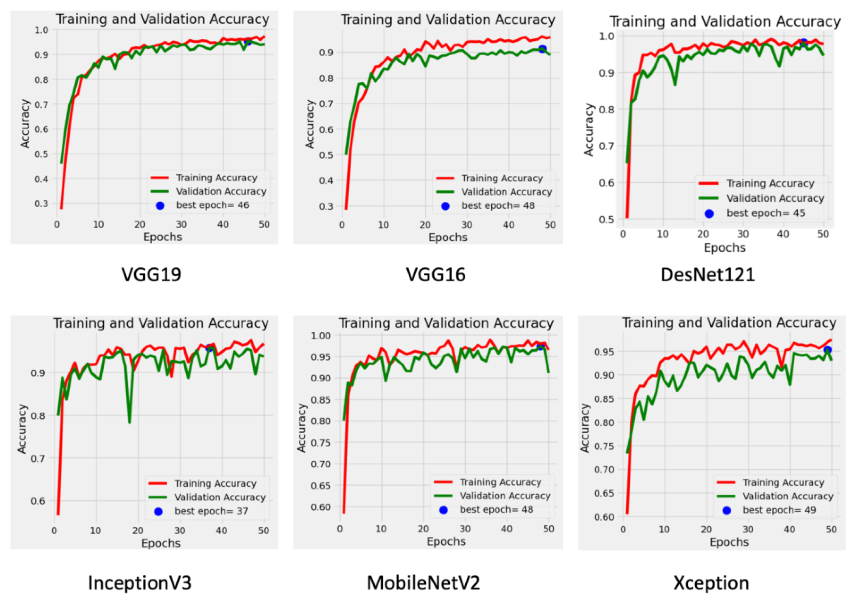
  • The created dataset was classified using deep learning models such as DenseNet121, VGG16, VGG19, InceptionV3, MobileNetV2, and Xception. The performance of these models was tested by combining them with various classification algorithms (k-NN, SVM, XGBOOST, and RF), and an increase in performance was observed.
  • A 95.76% accuracy rate was achieved by integrating the DenseNet121 model and the XGBOOST classification algorithm. This result shows the power of deep learning approaches in classifying chaotic systems.
  • This study shows that deep learning models can be used with high accuracy rates on the time series data of chaotic systems and provides an important basis for future studies in this field in the literature.
  • The method presented in this study and the results obtained contribute to a better understanding of chaotic systems and encourage the use of deep learning methods in this field in the future.
The other sections of this study are organized as follows:
In Section 2, the discrete-time chaotic systems, generated dataset, and deep learning models applied for classification are explained in detail. In Section 3, the proposed model is detailed. Section 4 evaluates the performances of the deep learning models, and their effects on the classification of chaotic systems are discussed. In Section 5, the general results of this study are summarized, the contributions of the findings to the field of chaotic systems and deep learning are emphasized, and suggestions for future studies are made.

2. Material and Methods

2.1. The Chaotic Systems Used and the Obtained Dataset

Discrete-time systems result from iterations of a suitable nonlinear function f ( x ) , often exhibiting feedback characteristics and producing chaotic behavior. Such systems are generally expressed as shown in Equation (1).
x n + 1 = f ( x n )
Here, x n + 1 represents the state of the system at the ( n + 1 ) -th iteration, while x n is the state at the n -th iteration. The function f ( x n ) defines the system’s dynamics, mapping the current state x n to the next state x n + 1 . The variable n refers to the discrete-time step or iteration count, and the function f ( x ) is typically nonlinear to exhibit chaotic behavior. For a system to be chaotic, f ( x ) must be highly sensitive to the initial conditions, meaning small differences in x n can lead to significantly different x n + 1 values over time, resulting in a wide range of possible states.
In this section, the dataset obtained from nine different discrete-time chaotic systems, namely the logistic map, sine map, tent map, cubic map, Ricker’s population model, Spence map, cusp map, Gauss map, and Pinchers map, are analyzed for the classification of the time series. The discrete-time chaotic systems used in this study are analyzed separately.
A logistic map is a mathematical model that studies discrete-time, one-dimensional deterministic chaotic systems. It was first introduced by Robert May in 1976. The formula for the logistic map is given in Equation (2) [29].
x n + 1 = a × x n ( 1 x n )
Here, x n represents the normalized population value at the n -th iteration, a is the system’s control parameter that influences the behavior of the system, and x n + 1 is the population state at the ( n + 1 ) -th iteration.
Figure 1 shows the time series of the logistic map obtained using the control parameters a = 3.7 , initial condition x 0 = 0.5 , and 100 iterations.
The sine map is a discrete-time and one-dimensional deterministic chaotic system. It exhibits chaotic behavior similar to the logistic map [30]. The general formula for the sine map is given in Equation (3) [31].
x n + 1 = a × s i n ( π × x n )
Here, x n represents the normalized value of the state of the system at the n -th iteration, a is the control parameter that influences the system’s behavior, and x n + 1 denotes the system’s state at the ( n + 1 ) -th iteration.
Figure 2 shows the time series of the sine map obtained with the control parameters a = 2.032 , initial condition x 0 = 0.5 , and 100 iterations.
The tent map is a discrete-time and one-dimensional chaotic system, and it is mathematically described by the formula given in Equation (4) [32].
x n + 1 = a × m i n ( x n , 1 x n )
Here, x n represents the normalized state of the system at the n -th iteration, a is the control parameter, and x n + 1 is the system’s state at the next iteration, determined by the function applied to x n and 1 x n
Figure 3 shows the time series of the Tent map obtained using the control parameters a = 1.89 , initial condition x 0 = 0.5 , and 100 iterations.
The cubic map is another discrete-time and one-dimensional mathematical model studied in the field of dynamical systems and chaos theory. The formula for the Cubic map is given in Equation (5) [33].
x n + 1 = a × x n × ( 1 x n 2 )
In this equation, x n represents the state of the system at the n -th iteration and a is the control parameter that governs the system’s behavior.
Figure 4 shows the time series of the Cubic map obtained with the control parameters a = 2.8938 , initial condition x 0 = 0.577 , and 100 iterations.
The Pinchers map is another discrete-time and one-dimensional mathematical model studied in the context of dynamical systems and chaos theory. The formula for the Pinchers map is given in Equation (6) [34].
x n + 1 = tanh s ( x n a )
Here, x n denotes the system’s state at the n -th iteration, while s and a are the control parameters. In this study, the parameter s is chosen as 2 .
Figure 5 shows the time series of the Pinchers map obtained with the control parameters s = 2.0 , a = 0.5 , initial condition x 0 = 0.5 , and 100 iterations.
The Spence map is a chaotic system first proposed by P.G. Spence. This map is a one-dimensional system defined as in Equation (7) [35].
x n + 1 = a × | l n x n |
Here, x n represents the state of the system at the n -th iteration and a is the control parameter that governs the system’s behavior.
Figure 6 shows the time series of the Spence map obtained with the control parameters a = 1.128 , initial condition x 0 = 2.388 , and 100 iterations.
The Cusp map is another important iterative map studied in chaotic systems and dynamical systems theory. This map is typically defined as in Equation (8) [36].
x n + 1 = 1 a × | x n |
Here, x n denotes the state of the system at the n -th iteration, while a is the control parameter that regulates the system’s behavior.
Figure 7 shows the time series of the Cusp map obtained with the control parameters a = 1.5 , initial condition x 0 = 0.555 , and 100 iterations.
The Ricker’s Population Model is a one-dimensional, discrete-time map developed by William E. Ricker in 1954 and used to model population dynamics [37]. The Ricker’s Population Model is defined as given in Equation (9).
x n + 1 = a × x n × e x n
Here, x n represents the state of the system at the n -th iteration, while a serves as the control parameter that governs the system’s behavior.
Figure 8 shows the time series of the Ricker’s Population Model with the control parameters a = 20 , initial condition x 0 = 1.0 , and 100 iterations.
The Gauss map is a discrete-time and chaotic system studied in connection with modular arithmetic and number theory. The Gauss map is defined by the formula given in Equation (10) [38].
x n + 1 = a x n m o d   1
Here, x n represents the state of the system at the n -th iteration, while a serves as the control parameter that governs the system’s behavior.
Figure 9 shows the time series of the Gaussian map obtained with the control parameters a = 1.7 , initial condition x 0 = 0.15 , and 100 iterations.

2.2. Procurement of the Dataset

This section explains in detail the process of creating the dataset used in this study. The dataset was created by iteratively solving discrete-time systems to calculate the state variables of each system and to obtain the corresponding time series. The values of both the system and the computational parameters were varied to diversify the time series data. The appropriate parameters were selected during the dataset’s creation to ensure that the time series were similar. With this approach, the classification problem was intended to be sufficiently challenging. For each time series, 1120 different results were obtained by varying the time series length, iteration count, control parameters, and initial conditions. In total, 10,080 images were obtained since nine different discrete-time chaotic systems were considered. The images were recorded in 256 × 256 dimensions and without grids.
The diversity and balance of the dataset were achieved by using different control parameters, initial conditions, iteration counts, and time series lengths for each discrete-time chaotic system. This diversification of the parameters provided a broad representation of each system’s dynamic behavior and added various variations to the dataset. This approach aims to improve the model’s overall performance by preventing it from overfitting a particular system.
The analyses were conducted over various parameters for each discrete-time chaotic system to create a diverse and representative dataset. The control parameters, initial conditions, and iteration counts were carefully varied in this context. By utilizing different combinations of initial conditions and control parameters for each system, the dynamic behaviors were diversified, reflecting a broad spectrum of behaviors for each system in the dataset.
Considering the time series lengths, each system’s representation across a wide variation range was ensured. This enabled the dataset to comprehensively and with balance represent the fundamental behavioral characteristics of each chaotic system in addressing the classification problem. Furthermore, an equal number of time series images from each system were included in the dataset to ensure a balanced representation of the classes, thus preventing the model from overfitting to a specific class. Consequently, this diversity strategy applied to the system parameters and initial conditions, combined with a balanced class distribution, ensured the dataset’s diversity and representativeness.
The dataset was created to address possible biases by considering a wide range of parameters without being limited to specific control parameters or initial conditions. This diversification was implemented to prevent the model from overfitting to a particular class or set of parameters and developing biases. Additionally, care was taken to ensure that the time series exhibited significant variation, allowing the model to learn balanced classes. These methods contribute to the model’s ability to exhibit more generalized and unbiased performance. Table 1 shows the values of the computational and system parameters used, while Table 2 shows some sample images and phase portraits of the time series obtained with the various parameters given in Table 1.

2.3. Deep Learning Models

This section details the deep learning models addressed, along with their benefits and applicability.
DenseNet121 is a variant of the DenseNet architecture proposed by Huang and colleagues in 2016 and presented in 2017. It operates on the principle of establishing dense connections between layers, where each layer takes the feature maps from previous layers as the input. This architecture strengthens the flow of information while alleviating the vanishing gradient problem. DenseNet121, with a total of 121 layers, enhances the model’s learning capacity while maintaining the parameter efficiency [39].
VGG19 and VGG16 is a deep neural network model developed by Karen Simonyan and Andrew Zisserman in 2014. This model achieved significant success in image recognition tasks using a structure composed of 19 layers. VGG19 presents a comprehensive evaluation of networks with increasing depth by utilizing very small (3 × 3) convolution filters. VGG16 is a deep neural network consisting of 16 layers. VGG16 and VGG19 are very similar; the only difference is the number of layers. The models demonstrated their potential in the field of visual recognition through their superior performance in the 2014 ImageNet Large Scale Visual Recognition Challenge (ILSVRC).
InceptionV3 is an advanced convolutional neural network model introduced by Christian Szegedy and his team in their 2015 paper. This model improves the overall performance by increasing the depth and breadth of the network and extracting richer features. The aim here is to use the added computation as efficiently as possible. A high performance is achieved with fewer parameters and lower computational requirements than previous models. For this reason, it is widely used in studies on deep learning [40].
MobileNetV2 offers an efficient network architecture with innovative features. The aim is to reduce computational costs and model complexity without compromising the model performance. MobileNetV2 sets a new standard for mobile devices while achieving high accuracy rates on large-scale datasets [41].
Xception is a more advanced version of the Inception architecture introduced by François Chollet in 2017. This architecture has approximately the same number of parameters as InceptionV3 but has achieved a higher classification accuracy on ImageNet and larger datasets. Since the model parameters are used more efficiently in the Xception architecture, the performance gains are greater than those of InceptionV3 [42].

2.4. Classification Algorithms

The machine learning methods used to classify a data point into predetermined classes with labeled training data are called classification algorithms. After training, the created model can classify new data points into the correct classes. This study selected the k-NN, SVM, XGBOOST, and RF algorithms as the classification algorithms.

2.4.1. K-Nearest Neighbors (k-NN) Algorithm

The K-NN algorithm is a classification method that classifies a data point by comparing it with its nearest neighbors. The K-NN considers the classes of the k nearest neighbors to determine the class of a data point, and the majority class of these neighbors is determined as the class of the new data. Although there are other distance measures, the Euclidean distance is generally used to measure the distance between data points. While the k-NN shows effective performance in small datasets due to its low computational cost, the computational load may increase and the performance may decrease in large datasets [43].
1.
The Euclidean distance is calculated as follows:
x , y = i = 1 n x i y i 2
Here, d ( x , y ) represents the distance between vectors x and y , where x i and y i are the i -th components of the vectors, and n denotes the dimensionality of the vectors.
2.
In the k-NN algorithm, the class of a test data point is determined by considering the class labels of the k nearest neighbors in the training dataset. The classification rule is expressed as follows:
y ^ = arg m a x y i = 1 k I y i = y
where
  • y ^ represents the predicted class.
  • y represents a class label.
  • k is the number of nearest neighbors considered in the classification.
  • I checks if y ^ belongs to class y . If the result is true, 1 is returned; otherwise, 0 is returned.

2.4.2. Support Vector Machine (SVM) Algorithm

An SVM is a frequently used method to find the best separating hyperplane for classifying data. This hyperplane is positioned to provide the maximum margin between two classes. Thus, the margin is maximized, while the classification errors are minimized. The SVM can also increase its flexibility with the kernel functions in nonlinear classification problems [44]. Therefore, it is often preferred when solving complex classification problems.
1.
The hyperplane separating the data is as follows:
w · x + b = 0
where
  • w is the weight vector (determining the direction of the hyperplane),
  • x is the input feature vector,
  • b is the bias term that determines the shift of the hyperplane from the origin.
2.
The optimization problem to find the optimal hyperplane is as follows:
m i n w , b 1 2 w 2
3.
Under the following conditions:
y i w x i + b 1 , i
where
  • w 2 is the squared norm of the weight vector, which is minimized to maximize the margin,
  • y i is the class label of the i-th training example, where y i ∈ {−1, 1},
  • x i is the feature vector of the i-th training example.

2.4.3. Random Forest (RF) Algorithm

An RF is a powerful machine learning algorithm that uses ensemble learning based on the principle of combining multiple structured decision trees to further increase the prediction accuracy. The RF improves the model’s overall performance by reducing the overfitting tendencies of the individual decision trees. Thanks to its parallel structure, it can be effectively used on large-sized datasets [45].
1.
Each decision tree usually uses the Gini index or Entropy.
G i n i D = 1 i = 1 C p i 2
E n t r o p y D = i = 1 C p i log 2 p i
where
  • G i n i ( D ) is the Gini index for dataset D , which measures the impurity or homogeneity of the dataset.
  • E n t r o p y ( D ) is the entropy of dataset D , representing the level of disorder or uncertainty in the data.
  • pi is the proportion of examples in class i.
  • C represents the total number of classes.
2.
The RF determines the final classification result by using the majority vote of the predictions made independently by each decision tree. The final classification for a data point x is performed as follows:
y ^ = Mode h 1 x , h 2 ( x ) , , h B x
Here, h i x represents the prediction made by the i -th tree, and B denotes the total number of trees. The final prediction y ^ is determined by the mode, which selects the most frequent class label among the predictions of all the B trees.

2.4.4. Extreme Gradient Boosting (XGBoost) Algorithm

XGBoost is a high-power, flexible machine learning method developed specifically to increase the predictive power of large datasets. In this method, each new tree works by correcting the errors of previous trees and preserving the decision trees that maintain the overall health of the model. XGBoost significantly reduces the programming time and prevents overfitting thanks to its parallel processing capability [46]. Due to these features, XGBoost has often been preferred to achieve the best results.
1.
The prediction function is as follows:
y ^ i = k = 1 K f k x i
Here, y ^ i represents the aggregated prediction for the i -th data point, where f k ( x i ) denotes the prediction made by the k -th decision tree for the same data point. The final prediction is obtained by summing the predictions of all the K decision trees.
2.
The loss function is as follows:
L ϕ = i = 1 n l y i , y ^ i + k = 1 k Ω f k
  • l y i , y ^ i is the loss function and Ω f k is the regularization term controlling the model complexity.
3.
The optimal weights are as follows:
w j * = G j H j + λ
Here, G j is the sum of the first derivatives, H j is the sum of the second derivatives, and λ is the regularization term that controls the model complexity.

3. Proposed Models

This study proposes various deep learning models for classifying the time series of discrete-time chaotic systems. The proposed models focus particularly on convolutional neural network (CNN)-based architectures. Since CNNs were quite successful in learning spatial hierarchies in image data, they were considered suitable for classifying the images obtained from the time series of chaotic systems. In this section, the details of the CNN models used and how these models classify the chaotic time series are discussed in detail, as presented in Figure 10.
The reason why we prefer the DenseNet121, VGG16, VGG19, InceptionV3, MobileNetV2, and Xception models in our study is that these models have proven themselves in the literature with their high success rates on time series classifications and chaotic systems. In particular, the dense interlayer connection structure of the DenseNet121 model strengthens the information flow and alleviates the vanishing gradient problem [39]. It is known that this model has a higher learning capacity compared to other models. In addition, the Xception model provides high performance with fewer parameters by increasing the parametric efficiency in deep learning architectures [42]. The MobileNetV2 model is optimized for mobile devices and lightweight applications with fewer computational power requirements and offers high accuracy rates on large datasets [41]. One of the reasons for choosing these models is that deep learning models can better understand the dynamic structures of chaotic systems. For example, the studies in the literature on the classification of chaotic time series have shown that such deep learning architectures achieve high accuracy rates. Neil et al. (2016) achieved an accuracy rate of 83.2% using a Phased LSTM model, but it was observed that the CNN-based models used in our study gave better results [18]. In addition, the applicability of these models was verified using performance metrics such as accuracy, sensitivity, specificity, and F1 scores in the training and testing processes. As mentioned in the discussion section, clearly shows that these models perform better than other methods in the literature. It was observed that our deep learning models were successful in comparative analyses with the other studies in the literature and made a significant contribution to the literature in the classification of chaotic time series.

4. Results and Discussion

This study used deep learning methods to classify the time series of nine different discrete-time chaotic systems. The dataset used in the experimental tests consists of time series images obtained from the relevant chaotic systems. The CNN models were trained and tested for the classification process. In this process, 70% of the images in the dataset were separated for training, 15% for testing, and 15% for validation. Various hyperparameters were determined to increase the model’s overall performance and provide an effective classification.
The dataset size to be trained in each iteration during the training process, namely, the mini-batch size value, was determined as 64. This choice ensured the model underwent a more balanced learning process and optimized the weights. The training process was performed over an epoch of 50 iterations, meaning the model was trained 50 times on the entire dataset.
In the optimization process, the Adam optimization algorithm was used. This algorithm was preferred to accelerate the learning and provide effective results, especially in large datasets and complex models. The learning rate value, which determines the learning speed, was set to 1 × 10⁻⁴. This low learning rate allowed the model to be optimized step by step, minimizing the risk of over-learning.
The main hyperparameters used in the training process included the learning rate, mini-batch size, and epoch number. The Adam optimization algorithm was preferred, especially for the optimization of the hyperparameters. Adam is a preferred method for large datasets and complex models in the literature and is known for providing fast learning and balanced results [47]. In our study, the learning rate was determined as 1 × 10⁻⁴. Choosing a low learning rate prevents over-learning (overfitting) by allowing the model to learn in smaller steps. In this way, the model could increase its overall performance without becoming overly sensitive to small changes in the dataset [48]. The mini-batch size was determined as 64, which aimed to provide balanced learning during the model’s training process. In addition, the model was trained for 50 epochs, and the performance of the model was monitored using the validation data in each epoch. Techniques such as grid search and random search were used to determine the best hyperparameter settings. These techniques helped us to optimize the model’s performance by systematically searching in the hyperparameter space [49]. In particular, the Adam optimizer allowed the efficient tuning of the hyperparameters, and the model performance was regularly evaluated based on the validation data.
Furthermore, the experimental studies were performed on a computer with an Apple M1 chip, using a graphics card with 8 GB RAM and 2 GB VRAM. While determining the model’s hyperparameters, the machine’s hardware features were considered. In this context, the model, which was optimized considering the hardware limitations, was designed with a structure to maximize the classification performance.
These details show that the methods used throughout this study were carefully selected, and the hardware and software optimizations were taken into account to increase the validity of the experimental results. The performances of the CNN models used in this study were evaluated on the test dataset after completing the training processes with the determined hyperparameters. The performance of each model was analyzed using various metrics, such as accuracy, sensitivity, specificity, precision, and F1 score. The equations for these metrics are given from (11) to (15). These analyses revealed the effectiveness of different CNN architectures in classifying the time series of chaotic systems.
A c c u r a c y = T P + T N T P + T N + F P + F N
S e n s i t i v i t y = T P T P + F N
S p e c i f i c i t y = T N T N + F P
P r e c i s i o n = T P T P + F P
F s c o r e = 2 T P 2 T P + F P + F N
In Table 3, the DenseNet121 model stood out as the model with the highest performance, with a 94.54% accuracy rate. This model also showed a balanced performance in all metrics with 100% sensitivity and 94.54% specificity rates. The VGG19 followed the DenseNet121 model among the other CNN models with a 94.09% accuracy rate. However, the VGG16 model showed a relatively lower performance with an accuracy rate of 88.83%, and it was observed that this model was less successful than the others.
The training and validation accuracy and training and validation loss graphs presented in Figure 11 and Figure 12 show the models’ performances during the training process. During the training process, the increase in the validation accuracy and the decrease in the loss function show that the models have successfully learned the dataset, and this learning process is efficient in terms of the model’s generalization.
As shown in Figure 13, the DenseNet121 model exhibited the highest performance despite having a more complex structure than the other models. Model complexity depends on factors such as the number of parameters and the layer depth. Complex models can be generalized better, especially on large and diverse datasets. However, this may not always be the case, and a careful balance must be struck between the model’s complexity and the risk of overfitting.
The results presented in Table 4 were obtained by testing the CNN models combined with different classification algorithms (SVM, XGBoost, RF, and KNN). These combinations showed a high performance, especially with the XGBoost algorithm. The combination of DenseNet121 and XGBoost provided the highest performance with an accuracy rate of 95.76%. This result shows that XGBoost is an effective classifier of the time series data of chaotic systems.
Figure 14 compares the accuracies achieved when different CNN models are combined with various classifiers. It clearly shows how the models, such as DenseNet121, VGG19, VGG16, InceptionV3, MobileNetV2, and Xception, perform with the SVM, XGBoost, RF, and KNN classifiers. This graph visualizes the accuracy achieved by each model when used with different classifiers.
In Figure 15, the DenseNet121 model achieved the highest F1 score when combined with XGBoost. This result revealed the accuracy rate and how well the model balanced false positives and negatives. Other CNN models also achieved similarly high F1 scores with XGBoost, but DenseNet121 showed the superior performance.
This study provides important findings in terms of comparing the results obtained in the classification of chaotic time series with deep learning models in previous studies. In the literature, the studies on the classification of chaotic systems have generally focused on the traditional machine learning methods or less complex deep learning models.
This current study successfully classified the time series of many chaotic systems using more advanced CNN models, and the accuracy rates were increased to over 95%. Particularly, when the DenseNet121 model was used with XGBoost, it provided a higher accuracy and F1 score compared to the results obtained through the previous studies. This can be associated with both the dataset’s diversity and the model’s complexity. Contrary to the results obtained with the traditional methods, this study shows that deep learning models provide higher success rates in chaotic time series.
As a further point, the findings of Figure 14 and Figure 15 reveal that using deep learning models, especially powerful classifiers such as XGBoost, for analyzing the time series of chaotic systems offers significant advantages over the existing methods in the literature. These results show that they have a higher accuracy and generalization capacity than the results reported in the previous studies. In the previous studies, mostly traditional methods or simpler Artificial Neural Networks (ANNs) were used to classify chaotic systems. Such studies generally achieved limited success rates due to the dataset sizes, the depth of the model used, and hardware limitations. The advanced CNN models and optimization techniques employed in the current study are observed to overcome these limitations and provide higher accuracy rates.
The DenseNet121 model achieved the highest accuracy rate when combined with XGBoost: 95.76%. This shows that XGBoost is an effective classifier on chaotic time series data and provides strong results when used with a complex model such as DenseNet121. On the other hand, when used with the KNN classifier, the performance of all the models decreased significantly, which reveals that the KNN algorithm is less effective on this type of data.
The high performance of the DenseNet121 model can be attributed to the dense connection structure of the model, the strong information flow between the layers, and its ability to provide better general learning for complex data. In particular, when integrated with the XGBOOST classification algorithm, the high accuracy rate of 95.76% reveals the strong classification ability of this method on chaotic time series data.
On the other hand, it was observed that the performances of the other models used in this study were lower compared to DenseNet121. This situation can be explained by the fact that the other models in this study could not learn the complexity of the dataset sufficiently due to the limited layer depth and less information transfer. For example, the generally lower performance of MobileNetV2, designed to be used in environments with limited hardware, such as mobile devices, compared to other models, can be explained by the simple structure of the model in question, which is not strong enough for chaotic systems.
The balance between the complexity of the models used in this article and computational efficiency is an important issue. Deep learning models such as DenseNet121 were preferred to increase the classification performance because these models can learn complex features thanks to deeper architectures. However, such deep architectures can have high computational costs in large datasets. Model complexity is directly proportional to the number of layers, the parameter amount, and the learning capacity of the model. In the DenseNet121 model, each layer uses the information from all the previous layers, allowing more parameters to be updated during the learning process and deeper features to be learned. However, this structure can increase the model’s training time and computational requirements. Since DenseNet121 consists of 121 layers, it may require higher computational power and memory capacity than other simpler models [39]. In our study, different optimization techniques were used to increase the computational efficiency of the model. For example, the mini-batch size was determined to be 64, which enabled the model to work more efficiently in the memory. In addition, the Adam optimization algorithm was preferred in the training process; this algorithm provides faster learning on large datasets by increasing computational efficiency [47]. In this way, the high performance offered by DenseNet121 was achieved by balancing the computational costs.
In addition, lighter models, such as MobileNetV2, were also evaluated in our study, and it was observed that these models provided reasonable accuracy rates with lower computational requirements [41]. However, models such as DenseNet121 and Xception, which are deeper and more powerful models on complex chaotic time series, provided higher accuracy rates. Therefore, a balance was established in our study in terms of both computational efficiency and classification performance. The trade-off between model complexity and computational efficiency was taken into account in our study, and high accuracy rates were achieved with the optimization strategies. Compared to other studies in the literature, it is seen that deep models such as DenseNet121 provide superior performance on more complex data structures, but computational costs should be managed carefully.
The risk of overfitting is a significant problem when working with deep learning models, and a number of strategies were used in our study to prevent this situation. First, various regularization techniques were applied during the training to prevent overfitting. In particular, the dropout method was used in the DenseNet121 and other CNN models. Dropout prevents the model from becoming overly dependent on only a certain subset of features by randomly disabling certain network neurons [50]. This allows the model to learn more generally and reduces the risk of overfitting. In addition, the early stopping strategy was used to prevent overfitting. The model’s performance was continuously monitored on the validation data throughout the training process, and the training was stopped when the validation loss started to increase at a certain point. This technique prevented the model from overtraining and performing poorly on the validation data [48]. Third, the hyperparameters such as the mini-batch size and learning rate were carefully adjusted during the training. In particular, a low learning rate (1 × 10⁻⁴) was selected, and the mini-batch size was set to 64. This low learning rate reduced the risk of overfitting by allowing the model to learn in smaller steps [47]. In addition, the dataset was kept large, and the generalization capacity of the model was increased by providing data diversity. The dataset used in our study consisted of 10,080 time series images obtained from different chaotic systems. This large dataset played an important role in preventing overfitting by allowing the model to learn different situations. At the same time, the diversity of the dataset was further increased by using data augmentation methods. To minimize the risk of overfitting, various regularization techniques (such as dropout and early stopping), the appropriate hyperparameter optimizations, and using a large dataset increased the model’s overall performance. These approaches achieved a high level of accuracy in deep models such as DenseNet121, while effective measures have been taken against the risk of over-learning.
Noisy data are inevitable when analyzing complex and dynamic structures, especially chaotic systems. In order to cope with such data and increase the generalization capacity of our models, several strategies were used in our study. Data augmentation techniques were applied during the training to increase the robustness of the model against noise. Data augmentation increases the model’s generalization ability against noisy or imperfect data by allowing the model to be trained on a larger, more diverse dataset [51]. In particular, techniques such as rotation, scaling, shifting, and adding random noise to the image were used. This way, the model achieved successful results on the ideal data and the data containing various distortions.
Regularization techniques such as dropout and L2 regularization were used to increase the robustness against noise. Dropout prevented the model from being overly dependent on certain features by disabling random neurons during the training and allowed the model to learn more general features [52]. L2 regularization, on the other hand, prevented the model from overfitting to the noisy data by limiting the size of the weights. The deep learning models proposed in our study were optimized to be robust against noisy and imperfect data. Data augmentation ensured that the accuracy rates remained high. In future studies, we aim to further improve the performance of the models by conducting more comprehensive tests on different types of noise.
The deep learning classification of chaotic systems can potentially be used in many theoretical and practical applications. In this study, from a theoretical perspective, a better understanding of the dynamic structures of chaotic systems is provided, and the effectiveness of deep learning approaches in classifying chaotic signals is revealed. In practical terms, it can be used in various areas, such as secure communications, data encryption, and biomedical applications. However, some difficulties may be encountered in real-world applications. In particular, due to the nonlinear nature of these systems, they need to be tested on larger datasets and more complex scenarios. However, research in this area must continue, and real-world application difficulties must be resolved.
In our study, the deep learning models used to achieve high accuracy rates were balanced with important factors such as computational cost and training time. In order to further clarify these issues, the performance of our model is detailed below in terms of computational cost and scalability. Among the deep learning models we used, DenseNet121, VGG16, VGG19, InceptionV3, MobileNetV2, and Xception, particularly more complex architectures such as DenseNet121, have higher computational costs. Since these models have more layers and parameters, they require higher computational power. However, in addition to these deep models that offer a high performance, lighter and faster models were also included in our study. For example, MobileNetV2 is a model optimized especially for mobile devices and platforms with limited resources and offers satisfactory accuracy rates with lower computational costs [41].
In addition, the transfer learning method was used to reduce the computational cost and provide a more efficient training process. Thanks to transfer learning, the training time is shortened and the costs are reduced using the weights of previously trained models [53]. Regarding the scalability of our model, various tests conducted on how the architectures used performed on large datasets. In particular, DenseNet121, despite having a more complex structure, offers a more efficient use of the parameters thanks to its dense connections between layers, which provides an advantage when scaling to larger datasets [39]. However, the training time and computational cost may increase when working with larger datasets. Strategies such as the appropriate division of the dataset (the use of the mini-batch) and parallel processing have been applied to balance this situation. In particular, the model’s training process can be accelerated, and more efficient scaling can be performed on large datasets using parallel processing (distributed computing) methods. In this way, the model’s applicability on larger datasets increases, and the efficient use of computational resources is provided [54]. The Adam optimization algorithm was used to optimize the training time. Adam accelerates the learning process and provides more effective learning in a shorter time [47]. In addition, the early stopping strategy was applied to prevent the overtraining of the model and unnecessary time loss. This strategy optimizes the training time by stopping the training when the model performance stabilizes at a certain level in the validation data [48]. GPU acceleration was also used to shorten the training time and reduce the computational cost in complex models. Deep learning models, in particular, work more efficiently on GPUs, and the training time is significantly reduced. Our study used a computer with an Apple M1 chip and a graphics card with 8 GB RAM. This hardware allowed us to develop a more efficient model by accelerating the training process. We utilized the following libraries during the study: NumPy (1.24.2), Pandas (1.5.3), Seaborn (0.12.2), Matplotlib (3.7.1), Scikit-learn (1.2.2), TensorFlow (2.13.0), and Keras (2.13.0). A balance was achieved between the computational cost, training time, and the accuracy of our study’s CNN models. Although more complex models, such as DenseNet121, had longer training times, they provided a high performance in terms of accuracy.
On the other hand, lighter models such as MobileNetV2 and InceptionV3 have shorter training times and lower computational costs while still providing high accuracy rates [40,41]. In our study, strategies were developed by considering factors such as the computational cost of the model, training time, and scalability. Lighter models (e.g., MobileNetV2), which provide more efficient solutions in terms of computational cost and training time, were used as viable alternatives without compromising the accuracy performance. At the same time, the scalability of the models that work efficiently on large datasets was increased, and parallel processing methods accelerated this process. Methods such as Adam optimization, early stopping, and GPU acceleration were successfully used to optimize training time and reduce costs.
Table 5 presents a comparative analysis between our study and other similar studies. In the study of Sun et al. (2024), the deterministic learning and k-means methods were used to classify chaotic systems, and an 84% accuracy rate was obtained. The methods used in this study generally focused on chaotic systems, which are simpler structures. However, the accuracy rate remained lower due to the structural simplicity of the model and limited data diversity [25]. In particular, the deterministic learning method used in the study of Sun et al. could not adapt deeply enough to the dynamic structure of chaotic systems. Therefore, the classification success was limited. Huang et al. (2020) used both a hybrid neural network and traditional prediction methods to predict chaotic time series. Their study’s 85.5% accuracy rate reveals the limitations of more traditional approaches used to classify chaotic systems [26]. Although hybrid methods successfully learn certain features of chaotic dynamics, the deep CNN models and classification algorithms used in our study in a hybrid manner achieved higher accuracy rates due to their deeper structures and wider learning capacities. This situation shows that deeper and more sophisticated deep learning models should replace traditional methods for analyzing chaotic systems. In the study of Boser et al. (1992), simple chaotic time series were classified using a Support Vector Machine (SVM), and an accuracy rate of 78.3% was obtained [44]. Although an SVM is an effective method in nonlinear classification problems, it could not provide a powerful enough approach for our study’s more complex chaotic systems. Unlike the SVM, the XGBoost algorithm used in our study provided better results because it eliminates classification errors with an iterative error correction process. The study of Boser et al. exhibited low performance, especially due to the limited dataset and the use of simpler chaotic systems. In the study conducted by Wyk and Steeb (1997), chaotic electronic systems were classified using classical neural network models. This study’s 75% accuracy rate shows how effective deep learning methods are in understanding chaotic time series [38]. Classical neural networks have difficulty in learning deeper features because they have a limited number of layers. In the study conducted by Neil et al. (2016), chaotic systems were classified on time series data using the Phased LSTM method. In this study, an accuracy rate of 83.2% was obtained [18]. Although a Phased LSTM is an effective method, especially for time series data with long-term dependencies, the learning capacity of the CNN-based architectures used in our study is higher. The limitations offered by the Phased LSTM can be explained by the fact that it cannot fully grasp the complexity that chaotic systems show over time. In contrast, the DenseNet121 model was able to better model the dynamics of chaotic systems by learning a wider range of features. The hybrid deep structures used in our study were much more successful in learning the complex dynamics of chaotic systems in particular. This comparison shows that deep learning models should replace classical methods.
One of the limitations of this study is that it is limited to certain chaotic systems only. In subsequent studies, adding new chaotic systems could diversify the dataset. In addition, the dataset size could be increased by using different initial conditions, control parameters, and iteration numbers. Future studies could be repeated by including more discrete-time chaotic systems in the dataset and increasing the dataset size.
In conclusion, this study has provided results that exceed the classification performances obtained by the existing methods in the literature. It proves that the time series of chaotic systems can be classified more effectively with deep learning techniques. In addition, these findings provide a new perspective in analyzing and classifying chaotic systems and a solid foundation for future research.

5. Conclusions

This study has attained high accuracy rates in the classification of the time series regarding nine different discrete-time chaotic systems. To increase the diversity of the dataset, chaotic systems were solved for different control parameters, initial conditions, and the number of iterations. As a result, a unique dataset containing a total of 10,080 time series images was created. The findings reveal that discrete-time chaotic systems can be classified efficiently and reliably over time series. This study’s most important finding is that the 95.76% accuracy rate was achieved by integrating the DenseNet121 model with the XGBOOST classification algorithm. Although other deep learning models have also yielded successful results, it has been shown that the models with deeper and stronger interlayer connections are more effective in classifying chaotic systems. These results show that deep learning algorithms can successfully realize the study of the complex dynamical structures of chaotic systems through visual representations. In addition, this work offers a more flexible and powerful approach to describing and analyzing chaotic systems compared to traditional methods.
In this study, the classification of the time series from nine different discrete-time chaotic systems was successfully accomplished using deep learning methods, specifically Convolutional Neural Networks (CNNs) combined with various classification algorithms such as Support Vector Machines (SVMs), XGBoost, Random Forest (RF), and K-Nearest Neighbors (KNN). The CNN models employed in this study, including DenseNet121, VGG19, VGG16, InceptionV3, MobileNetV2, and Xception, demonstrated a high accuracy in classifying chaotic time series. Combining these CNN models with advanced classification algorithms, particularly XGBoost, resulted in enhanced performance, with DenseNet121 coupled with XGBoost achieving the highest accuracy.
To increase the diversity of the dataset, chaotic systems were solved with varying control parameters, initial conditions, and numbers of iterations, creating a unique dataset comprising a total of 10,080 time series images. The findings from this study indicate that discrete-time chaotic systems can be effectively and reliably classified using these deep learning methods and classification algorithms. The use of CNNs, in combination with classification algorithms, has proven to be a powerful approach for analyzing and identifying the complex dynamical structures of chaotic systems with a high level of accuracy.
Based on these considerations and contributions, this work demonstrates the effectiveness of CNN-based deep learning models in chaos theory by introducing a more flexible and robust approach compared to traditional methods for describing and analyzing chaotic systems. The successful integration of classification algorithms with CNNs in this context offers significant contributions to the fields of chaos theory, machine learning, and computational modeling.
Accordingly, future research could explore several directions to advance the findings of this study further. First, expanding the dataset by including additional chaotic systems and increasing the complexity of the time series data could provide a more comprehensive evaluation of the proposed models. Additionally, experimenting with other deep learning architectures, such as Recurrent Neural Networks (RNNs) and Long Short-Term Memory (LSTM) networks, which are particularly well suited for sequential data, could offer further improvements in classification accuracy. Moreover, optimizing the models for real-time applications and deploying them on more advanced hardware could enhance their applicability in practical scenarios. Investigating the use of ensemble methods, where multiple models are combined to make predictions, could also provide a boost in performance and robustness. Finally, applying these models to real-world chaotic systems in various fields, such as finance, biology, or meteorology, could validate their effectiveness in practical applications and lead to new insights into the behaviors and patterns of chaotic systems.

Author Contributions

The authors have equally contributed to this paper. All authors have read and agreed to the published version of the manuscript.

Funding

The authors received no specific funding for this study.

Data Availability Statement

The data will be made available by the authors on request.

Conflicts of Interest

The authors declare no competing interests.

References

  1. Umar, T.; Nadeem, M.; Anwer, F. A new modified Skew Tent Map and its application in pseudo-random number generator. Comput. Stand. Interfaces 2024, 89, 103826. [Google Scholar] [CrossRef]
  2. Murillo-Escobar, D.; Vega-Pérez, K.; Murillo-Escobar, M.A.; Arellano-Delgado, A.; López-Gutiérrez, R.M. Comparison of two new chaos-based pseudorandom number generators implemented in microcontroller. Integration 2024, 96, 102130. [Google Scholar] [CrossRef]
  3. Emin, B.; Akgul, A.; Horasan, F.; Gokyildirim, A.; Calgan, H.; Volos, C. Secure Encryption of Biomedical Images Based on Arneodo Chaotic System with the Lowest Fractional-Order Value. Electronics 2024, 13, 2122. [Google Scholar] [CrossRef]
  4. Li, L. A novel chaotic map application in image encryption algorithm. Expert Syst. Appl. 2024, 252, 124316. [Google Scholar] [CrossRef]
  5. Kıran, H.E. A Novel Chaos-Based Encryption Technique with Parallel Processing Using CUDA for Mobile Powerful GPU Control Center. Chaos Fractals 2024, 1, 6–18. [Google Scholar] [CrossRef]
  6. Patidar, V.; Kaur, G. Lossless Image Encryption using Robust Chaos-based Dynamic DNA Coding, XORing and Complementing. Chaos Theory Appl. 2023, 5, 178–187. [Google Scholar] [CrossRef]
  7. Aparna, H.; Madhumitha, J. Combined image encryption and steganography technique for enhanced security using multiple chaotic maps. Comput. Electr. Eng. 2023, 110, 108824. [Google Scholar] [CrossRef]
  8. Hue, T.T.K.; Linh, N.T.; Nguyen-Duc, M.; Hoang, T.M. Data Hiding in Bit-plane Medical Image Using Chaos-based Steganography. In Proceedings of the 2021 International Conference on Multimedia Analysis and Pattern Recognition (MAPR), Virtual Conference, 15–16 October 2021; pp. 1–6. [Google Scholar]
  9. Rahman, Z.-A.S.A.; Jasim, B.H. Hidden Dynamics Investigation, Fast Adaptive Synchronization, and Chaos-Based Secure Communication Scheme of a New 3D Fractional-Order Chaotic System. Inventions 2022, 7, 108. [Google Scholar] [CrossRef]
  10. Nguyen, Q.D.; Giap, V.N.; Tran, V.H.; Pham, D.-H.; Huang, S.-C. A Novel Disturbance Rejection Method Based on Robust Sliding Mode Control for the Secure Communication of Chaos-Based System. Symmetry 2022, 14, 1668. [Google Scholar] [CrossRef]
  11. Reddy, N.; Sadanandachary, A. A Secure Communication System of Synchronized Chua’s Circuits in LC Parallel Coupling. Chaos Theory Appl. 2023, 5, 167–177. [Google Scholar] [CrossRef]
  12. Ayubi, P.; Jafari Barani, M.; Yousefi Valandar, M.; Yosefnezhad Irani, B.; Sedagheh Maskan Sadigh, R. A new chaotic complex map for robust video watermarking. Artif. Intell. Rev. 2021, 54, 1237–1280. [Google Scholar] [CrossRef]
  13. Kumar, S.; Chauhan, A.; Alam, K. Weighted and Well-Balanced Nonlinear TV-Based Time-Dependent Model for Image Denoising. Chaos Theory Appl. 2023, 5, 300–307. [Google Scholar] [CrossRef]
  14. Girshick, R.; Donahue, J.; Darrell, T.; Malik, J. Rich feature hierarchies for accurate object detection and semantic segmentation. In Proceedings of the IEEE Conference on Computer Vision and Pattern Recognition, Boston, MA, USA, 7–12 June 2014; pp. 580–587. [Google Scholar] [CrossRef]
  15. Dahl, G.E.; Yu, D.; Deng, L.; Acero, A. Context-dependent pre-trained deep neural networks for large-vocabulary speech recognition. IEEE Trans. Audio Speech Lang. Process. 2012, 20, 30–42. [Google Scholar] [CrossRef]
  16. Mikolov, T.; Chen, K.; Corrado, G.; Dean, J. Efficient estimation of word representations in vector space. arXiv 2013, arXiv:1301.3781. [Google Scholar]
  17. Ravi, D.; Wong, C.; Deligianni, F.; Berthelot, M.; Andreu-Perez, J.; Lo, B.; Yang, G.Z. Deep Learning for Health Informatics. IEEE J. Biomed. Health Inform. 2017, 21, 4–21. [Google Scholar] [CrossRef]
  18. Neil, D.; Pfeiffer, M.; Liu, S.-C. Phased LSTM: Accelerating Recurrent Network Training for Long or Event-based Sequences. In Advances in Neural Information Processing Systems; Lee, D., Sugiyama, M., Luxburg, U., Guyon, I., Garnett, R., Eds.; Curran Associates, Inc.: Red Hook, NY, USA, 2016; Volume 29. [Google Scholar]
  19. Habib, Z.; Khan, J.S.; Ahmad, J.; Khan, M.A.; Khan, F.A. Secure speech communication algorithm via DCT and TD-ERCS chaotic map. In Proceedings of the 2017 4th International Conference on Electrical and Electronic Engineering (ICEEE), Ankara, Turkey, 8–10 April 2017; pp. 246–250. [Google Scholar] [CrossRef]
  20. Boullé, N.; Dallas, V.; Nakatsukasa, Y.; Samaddar, D. Classification of Chaotic Time Series with Deep Learning; Elsevier: Amsterdam, The Netherlands, 2020. [Google Scholar]
  21. Jia, B.; Wu, H.; Guo, K. Chaos theory meets deep learning: A new approach to time series forecasting. Expert Syst. Appl. 2024, 255, 124533. [Google Scholar] [CrossRef]
  22. Aricioğlu, B.; Uzun, S.; Kaçar, S. Deep learning based classification of time series of Chen and Rössler chaotic systems over their graphic images. Phys. D Nonlinear Phenom. 2022, 435, 133306. [Google Scholar] [CrossRef]
  23. Uzun, S.; Kaçar, S.; Ar\ic\io\uglu, B. Deep learning based classification of time series of chaotic systems over graphic images. Multimed. Tools Appl. 2024, 83, 8413–8437. [Google Scholar] [CrossRef]
  24. Pourafzal, A.; Fereidunian, A.; Safarihamid, K. Chaotic Time Series Recognition: A Deep Learning Model Inspired by Complex Systems Characteristics. Int. J. Eng. Trans. A Basics 2023, 36, 1–9. [Google Scholar] [CrossRef]
  25. Sun, C.; Wu, W.; Zhang, Z.; Li, Z.; Ji, B.; Wang, C. Time series clustering of dynamical systems via deterministic learning. Int. J. Mach. Learn. Cybern. 2024, 15, 2761–2779. [Google Scholar] [CrossRef]
  26. Huang, W.; Li, Y.; Huang, Y. Deep Hybrid Neural Network and Improved Differential Neuroevolution for Chaotic Time Series Prediction. IEEE Access 2020, 8, 159552–159565. [Google Scholar] [CrossRef]
  27. Akgöz, B.; Civalek, Ö. Buckling Analysis of Functionally Graded Tapered Microbeams via Rayleigh–Ritz Method. Mathematics 2022, 10, 4429. [Google Scholar] [CrossRef]
  28. Le Berre, S.; Ramière, I.; Fauque, J.; Ryckelynck, D. Condition Number and Clustering-Based Efficiency Improvement of Reduced-Order Solvers for Contact Problems Using Lagrange Multipliers. Mathematics 2022, 10, 1495. [Google Scholar] [CrossRef]
  29. May, R.M. Simple mathematical models with very complicated dynamics. Nature 1976, 261, 459–467. [Google Scholar] [CrossRef] [PubMed]
  30. Pak, C.; An, K.; Jang, P.; Kim, J.; Kim, S. A novel bit-level color image encryption using improved 1D chaotic map. Multimed. Tools Appl. 2019, 78, 12027–12042. [Google Scholar] [CrossRef]
  31. Strogatz, S.H. Nonlinear Dynamics and Chaos: With Applications to Physics, Biology, Chemistry, and Engineering, 2nd ed.; Westview Press, a Member of the Perseus Books Group, [2015]: Boulder, CO, USA, 1994. [Google Scholar]
  32. Devaney, R.L. An Introduction to Chaotic Dynamical Systems, 2nd ed.; Addison-Wesley: Redwood City, CA, USA, 1984; ISBN 978-0201156808. [Google Scholar]
  33. Wan-Zhen, Z.; Ming-Zhou, D.; Jia-Nan, L. Symbolic description of periodic windows in the antisymmetric cubic map. Chin. Phys. Lett. 1985, 2, 293. [Google Scholar] [CrossRef]
  34. Potapov, A.; Ali, M. Robust chaos in neural networks. Phys. Lett. A 2000, 277, 310–322. [Google Scholar] [CrossRef]
  35. Shaw, R. Strange Attractors, Chaotic Behavior, and Information Flow. Z. Naturforschung A 1981, 36, 80–112. [Google Scholar] [CrossRef]
  36. Beck, C.; Schlögl, F. Thermodynamics of Chaotic Systems; Cambridge University Press: New York, NY, USA, 1995. [Google Scholar]
  37. Ricker, W.E. Stock and Recruitment. J. Fish. Res. Board Canada 1954, 11, 559–623. [Google Scholar] [CrossRef]
  38. Van Wyk, M.A.; Steeb, W.-H. Chaos in Electronics; Kluwer Academic Publishers: Dordrecht, The Netherlands, 1997. [Google Scholar]
  39. Huang, G.; Liu, Z.; Van Der Maaten, L.; Weinberger, K.Q. Densely connected convolutional networks. In Proceedings of the IEEE Conference on Computer Vision and Pattern Recognition, Honolulu, HI, USA, 21–26 July 2017; pp. 4700–4708. [Google Scholar]
  40. Szegedy, C.; Vanhoucke, V.; Ioffe, S.; Shlens, J.; Wojna, Z. Rethinking the Inception Architecture for Computer Vision. In Proceedings of the IEEE Conference on Computer Vision and Pattern Recognition, Las Vegas, NV, USA, 27–30 June 2016; pp. 2818–2826. [Google Scholar] [CrossRef]
  41. Sandler, M.; Howard, A.; Zhu, M.; Zhmoginov, A. Mobilenetv2: Inverted residuals and linear bottlenecks. arXiv 2018, arXiv:1801.04381. [Google Scholar]
  42. Chollet, F. Xception: Deep learning with depthwise separable convolutions. In Proceedings of the IEEE Conference on Computer Vision and Pattern Recognition, Honolulu, HI, USA, 21–26 July 2017; pp. 1251–1258. [Google Scholar]
  43. Cover, T.; Hart, P. Nearest neighbor pattern classification. IEEE Trans. Inf. Theory 1967, 13, 21–27. [Google Scholar] [CrossRef]
  44. Boser, B.E.; Guyon, I.M.; Vapnik, V.N. A training algorithm for optimal margin classifiers. In Proceedings of the 5th Annual ACM Workshop on Computational Learning Theory, Pittsburgh, PA, USA, 27–29 July 1992; pp. 144–152. [Google Scholar]
  45. Breiman, L. Random forests. Mach. Learn. 2001, 45, 5–32. [Google Scholar] [CrossRef]
  46. Chen, T.; Guestrin, C. XGBoost: A Scalable Tree Boosting System. In Proceedings of the 22nd ACM SIGKDD International Conference on Knowledge Discovery and Data Mining, San Francisco, CA, USA, 13–17 August 2016. [Google Scholar] [CrossRef]
  47. Kingma, D.P.; Ba, J. Adam: A method for stochastic optimization. arXiv 2015, arXiv:1412.6980. [Google Scholar]
  48. Goodfellow, I.; Bengio, Y.; Courville, A. Deep Learning; MIT Press: Cambridge, MA, USA, 2016. [Google Scholar]
  49. Bergstra, J.; Bengio, Y. Random search for hyper-parameter optimization. J. Mach. Learn. Res. 2012, 13, 281–305. [Google Scholar]
  50. Selvaraju, R.R.; Cogswell, M.; Das, A.; Vedantam, R.; Parikh, D.; Batra, D. Grad-CAM: Visual explanations from deep networks via gradient-based localization. In Proceedings of the IEEE International Conference on Computer Vision, Venice, Italy, 22–29 October 2017; pp. 618–626. [Google Scholar]
  51. Shorten, C.; Khoshgoftaar, T.M. A survey on image data augmentation for deep learning. J. Big Data 2019, 6, 1–48. [Google Scholar] [CrossRef]
  52. Srivastava, N.; Hinton, G.; Krizhevsky, A.; Sutskever, I.; Salakhutdinov, R. Dropout: A simple way to prevent neural networks from overfitting. J. Mach. Learn. Res. 2014, 15, 1929–1958. [Google Scholar]
  53. Pan, S.J.; Yang, Q. A Survey on Transfer Learning. IEEE Trans. Knowl. Data Eng. 2010, 22, 1345–1359. [Google Scholar] [CrossRef]
  54. Dean, J.; Corrado, G.S.; Monga, R.; Chen, K.; Devin, M.; Le, Q.V.; Mao, M.R.; Senior, A.; Tucker, P.; Yang, K.; et al. Large scale distributed deep networks. In Advances in Neural Information Processing Systems; National Poisons Information Service: NPIS: Birmingham, UK, 2012; pp. 1223–1231. [Google Scholar]
Figure 1. Time series of the logistic map obtained after 100 iterations with the control parameters a = 3.7 and initial condition x 0 = 0.5 .
Mathematics 12 03052 g001
Figure 2. Time series of the Sine map obtained after 100 iterations with the control parameters a = 2.032 and initial condition x 0 = 0.5 .
Mathematics 12 03052 g002
Figure 3. Time series of the Tent map obtained after 100 iterations with the control parameters a = 1.89 and initial condition x 0 = 0.5 .
Mathematics 12 03052 g003
Figure 4. Time series of the Cubic map obtained after 100 iterations with the control parameters a = 2.8938 and initial condition x 0 = 0.577 .
Mathematics 12 03052 g004
Figure 5. Time series of the Pinchers map obtained after 100 iterations with the control parameters s = 2.0, a = 0.5 , and initial condition x 0 = 0.5 .
Mathematics 12 03052 g005
Figure 6. Time series of the Spence map obtained after 100 iterations with the control parameters a = 1.128 and initial condition x 0 = 2.388 .
Mathematics 12 03052 g006
Figure 7. Time series of the Cusp map obtained after 100 iterations with the control parameters a = 1.5 and initial condition x 0 = 0.555 .
Mathematics 12 03052 g007
Figure 8. Time series of the Ricker’s Population Model obtained after 100 iterations with the control parameters a = 20 and initial condition x 0 = 1.0 .
Mathematics 12 03052 g008
Figure 9. Time series of the Gaussian map obtained after 100 iterations with the control parameters a = 1.7 and initial condition x 0 = 0.15 .
Mathematics 12 03052 g009
Figure 10. Overall structural design of the proposed model.
Mathematics 12 03052 g010
Figure 11. Training and validation accuracy performance results of CNN models on discrete-time chaos images.
Mathematics 12 03052 g011
Figure 12. Training and validation loss performance results of CNN models on discrete-time chaos images.
Mathematics 12 03052 g012
Figure 13. Complexity results of CNN models on discrete-time chaos images.
Mathematics 12 03052 g013
Figure 14. Comparative accuracy of CNN models with different classifiers.
Mathematics 12 03052 g014
Figure 15. F1 score comparison between CNN models.
Mathematics 12 03052 g015
Table 1. The calculation and system parameters utilized.
SystemControl Parameters (a)Number of IterationsThe Initial Conditions
Logistic map[3.6, 3.626, 3.652, 3.678, 3.704, 3.73, 3.756, 3.782, 3.808, 3.834, 3.86, 3.886, 3.912, 3.938, 3.964, 3.99]100
150
200
250
300
[0.1, 0.1572, 0.2144, 0.2716, 0.3288, 0.386, 0.4432, 0.5004, 0.5576, 0.6148, 0.672, 0.7292, 0.7864, 0.8436]
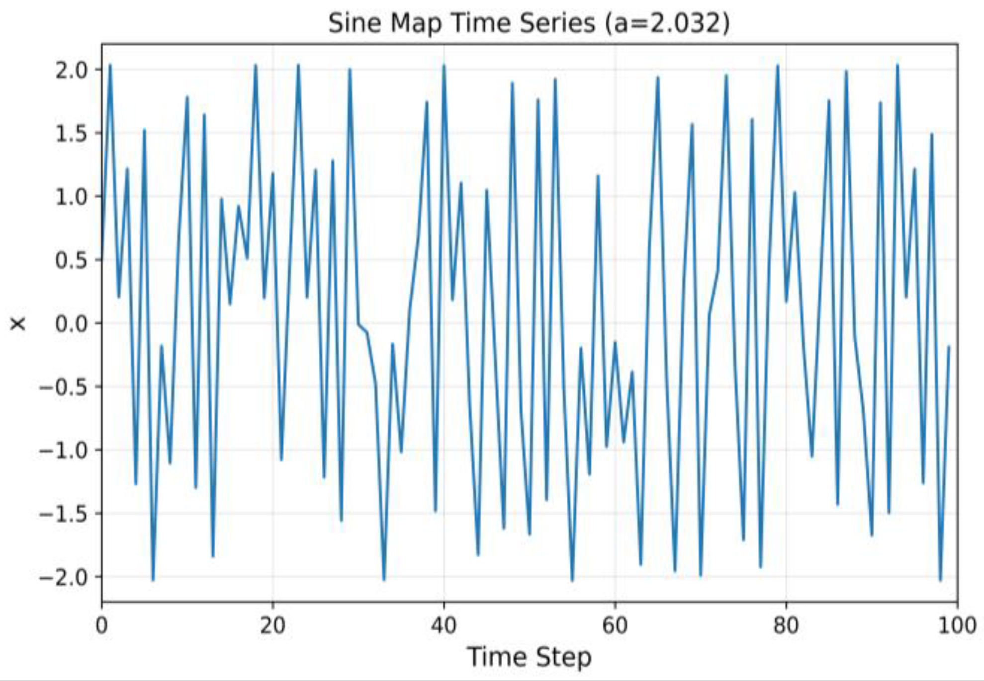
Sine map[2.0, 2.032, 2.064, 2.096, 2.128, 2.16, 2.192, 2.224, 2.256, 2.288, 2.32, 2.352, 2.384, 2.416, 2.448, 2.48][−1.0, −0.857, −0.714, −0.571, −0.428, −0.285, −0.142, 0.001, 0.144, 0.287, 0.43, 0.573, 0.716, 0.859]
Tent map[1.5, 1.526, 1.552, 1.578, 1.604, 1.63, 1.656, 1.682, 1.708, 1.734, 1.76, 1.786, 1.812, 1.838, 1.864, 1.89][0.1, 0.165, 0.23, 0.295, 0.36, 0.425, 0.49, 0.555, 0.62, 0.685, 0.75, 0.815, 0.88, 0.945]
Cubic map[2.88, 2.8869, 2.8938, 2.9007, 2.9076, 2.9145, 2.9214, 2.9283, 2.9352, 2.9421, 2.949, 2.9559, 2.9628, 2.9697, 2.9766, 2.9835][0.1, 0.153, 0.206, 0.259, 0.312, 0.365, 0.418, 0.471, 0.524, 0.577, 0.63, 0.683, 0.736, 0.789]
Pinchers map[0.49, 0.4938, 0.4976, 0.5014, 0.5052, 0.509, 0.5128, 0.5166, 0.5204, 0.5242, 0.528, 0.5318, 0.5356, 0.5394, 0.5432, 0.547][0.0, 0.072, 0.144, 0.216, 0.288, 0.36, 0.432, 0.504, 0.576, 0.648, 0.72, 0.792, 0.864, 0.936]
Spence map[0.9, 0.957, 1.014, 1.071, 1.128, 1.185, 1.242, 1.299, 1.356, 1.413, 1.47, 1.527, 1.584, 1.641, 1.698, 1.755][0.1, 0.308, 0.516, 0.724, 0.932, 1.14, 1.348, 1.556, 1.764, 1.972, 2.18, 2.388, 2.596, 2.804]
Cusp map[1.5, 1.5256, 1.5512, 1.5768, 1.6024, 1.628, 1.6536, 1.6792, 1.7048, 1.7304, 1.756, 1.7816, 1.8072, 1.8328, 1.8584, 1.884][0.1, 0.165, 0.23, 0.295, 0.36, 0.425, 0.49, 0.555, 0.62, 0.685, 0.75, 0.815, 0.88, 0.945]
Ricker’s Population Model[19.0, 19.126, 19.252, 19.378, 19.504, 19.63, 19.756, 19.882, 20.008, 20.134, 20.26, 20.386, 20.512, 20.638, 20.764, 20.89][1.0, 1.072, 1.144, 1.216, 1.288, 1.36, 1.432, 1.504, 1.576, 1.648, 1.72, 1.792, 1.864, 1.936]
Gauss map[1.7, 1.7076, 1.7152, 1.7228, 1.7304, 1.738, 1.7456, 1.7532, 1.7608, 1.7684, 1.776, 1.7836, 1.7912, 1.7988, 1.8064, 1.814][0.15, 0.176, 0.202, 0.228, 0.254, 0.28, 0.306, 0.332, 0.358, 0.384, 0.41, 0.436, 0.462, 0.488]
Table 2. Some sample images and phase portraits obtained from the time series of the discrete-time chaotic systems.
Time SeriesPhase Portrait
Logistic mapMathematics 12 03052 i001Mathematics 12 03052 i002Mathematics 12 03052 i003Mathematics 12 03052 i004Mathematics 12 03052 i005
Sine mapMathematics 12 03052 i006Mathematics 12 03052 i007Mathematics 12 03052 i008Mathematics 12 03052 i009Mathematics 12 03052 i010
Tent mapMathematics 12 03052 i011Mathematics 12 03052 i012Mathematics 12 03052 i013Mathematics 12 03052 i014Mathematics 12 03052 i015
Cubic mapMathematics 12 03052 i016Mathematics 12 03052 i017Mathematics 12 03052 i018Mathematics 12 03052 i019Mathematics 12 03052 i020
Pinchers mapMathematics 12 03052 i021Mathematics 12 03052 i022Mathematics 12 03052 i023Mathematics 12 03052 i024Mathematics 12 03052 i025
Spence mapMathematics 12 03052 i026Mathematics 12 03052 i027Mathematics 12 03052 i028Mathematics 12 03052 i029Mathematics 12 03052 i030
Cusp mapMathematics 12 03052 i031Mathematics 12 03052 i032Mathematics 12 03052 i033Mathematics 12 03052 i034Mathematics 12 03052 i035
Ricker’s population modelMathematics 12 03052 i036Mathematics 12 03052 i037Mathematics 12 03052 i038Mathematics 12 03052 i039Mathematics 12 03052 i040
Gauss mapMathematics 12 03052 i041Mathematics 12 03052 i042Mathematics 12 03052 i043Mathematics 12 03052 i044Mathematics 12 03052 i045
Table 3. The performance results of CNN models on discrete-time chaos images.
CNN ModelsAccuracySensitivitySpecificityPrecisionF1 Score
DenseNet1210.94541.0000.94540.94540.9454
VGG190.94091.0000.94090.94090.9409
VGG160.88831.0000.88830.94090.9139
InceptionV30.93701.0000.93700.94090.9389
MobileNetV20.91071.0000.91070.94090.9255
Xception0.93001.0000.93000.94090.9354
Table 4. Experimental test results with CNNs and classification.
CNN ModelsClassificationAccuracySensitivitySpecificityPrecisionF1 Score
DenseNet121SVM0.93351.0000.99661.0000.9983
XGBOOST0.95761.0001.0001.0001.000
RF0.92221.0000.99661.0000.9983
KNN0.86441.0001.0001.0001.000
VGG19SVM0.86301.0001.0001.0001.000
XGBOOST0.93151.0001.0001.0001.000
RF0.88720.99671.0000.99650.9982
KNN0.86171.0001.0001.0001.000
VGG16SVM0.86341.0001.0001.0001.000
XGBOOST0.92221.0001.0001.0001.000
RF0.88491.0001.0001.0001.000
KNN0.85681.0001.0001.0001.000
InceptionV3SVM0.83891.0001.0001.0001.000
XGBOOST0.80851.0000.99591.0000.9979
RF0.71821.0001.0001.0001.000
KNN0.72350.99670.99580.99580.9958
MobileNetV2SVM0.88851.0001.0001.0001.000
XGBOOST0.87531.0001.0001.0001.000
RF0.79030.99330.99610.99230.9942
KNN0.74800.99641.0000.99600.9980
XceptionSVM0.90871.0001.0001.0001.000
XGBOOST0.89021.0001.0001.0001.000
RF0.82141.0001.0001.0001.000
KNN0.78140.99360.99230.99230.9923
Table 5. Comparison of the proposed model with other studies.
AuthorsMethodsChaotic SystemsAcc (%)
2024, Sun et al. [25]Deterministic learning + k-meansLorenz, Rossler84.00
2020, Huang et al. [26]Hybrid Neural Network +Traditional forecastingChaotic time series85.50
2016, Neil et al. [18]Phased LSTM (Classifying chaotic systems with time series data)Various chaotic time series83.20
1992, Boser et al. [44]SVM (with a basic chaotic time series)Chaotic Electronic Systems78.30
1997, Wyk, Steeb, et al. [38]Chaos in Electronics (Classic neural network models)Chaotic Electronic Systems75.00
2024, this paperCNN models (DenseNet121, VGG19, VGG16, InceptionV3, MobileNetV2, and Xception) + classification algorithms (SVM, XGBOOST, RF, and KNN)Logistic ap, Sine Map, Tent Map, etc.95.76
Disclaimer/Publisher’s Note: The statements, opinions and data contained in all publications are solely those of the individual author(s) and contributor(s) and not of MDPI and/or the editor(s). MDPI and/or the editor(s) disclaim responsibility for any injury to people or property resulting from any ideas, methods, instructions or products referred to in the content.

