Solitons, Lumps, Breathers, and Interaction Phenomena for a (2+1)-Dimensional Variable-Coefficient Extended Shallow-Water Wave Equation

Abstract

In this paper, soliton solutions, lump solutions, breather solutions, and lump-solitary wave solutions of a (2+1)-dimensional variable-coefficient extended shallow-water wave (vc-eSWW) equation are obtained based on its bilinear form. By calculating the vector field of the potential function, the interaction between lump waves and solitary waves is studied in detail. Lumps can emerge from the solitary wave and are semi-localized in time. The analytical solutions may enrich our understanding of the nature of shallow-water waves.

1. Introduction

Various types of waves, influenced by different physical factors, exist in the ocean, with shallow-water waves describing the dynamics of water movement when the water depth is less than half the wavelength [1,2]. The shallow-water wave (SWW) equation, derived from Navier–Stokes equations, is applied to investigate surface waves in shallow water [3]. In its unidirectional form, the shallow-water equation is known as the Saint–Venant equations, which is widely applied to analyze water flow in open channels [4,5].

In nonlinear science, the SWW equation is also a significant research focus. In 1895, the Korteweg–de Vries (KdV) equation was introduced to study solitary waves in shallow water [6]. The Kadomtsev–Petviashvili (KP) equation, which describes the evolution of long water waves and small-amplitude surface waves with weak nonlinearity, dispersion, and perturbation in the y-direction, is one of the most notable generalizations of the KdV equation in (2+1) dimensions [7].

In 1986, Boiti proposed another generalization of the KdV equation, known as the extended shallow-water wave (eSWW) equation, which represents the KdV equation in two spatial dimensions [8]. To obtain this generalization, the Lax representation is introduced as follows:

$$[T_1,T_2]\psi =0,$$

(1)

where

$$\begin{array}{cc}\hfill T_1& ={\partial }_x^2-{\partial }_y^2+p(x,y,t),\hfill \\ \hfill T_2& ={\partial }_t+V({\displaystyle \frac{\partial }{\partial x}},{\displaystyle \frac{\partial }{\partial y}},p),\hfill \end{array}$$

(2)

and $\psi$ is the solution of the spectral function

$$T_1\psi =0.$$

(3)

Applying the coordinate transformation $\lambda ={\displaystyle \frac{1}{2}}(x+y)$ and $\mu ={\displaystyle \frac{1}{2}}(x-y)$, and after simplification, the eSWW equation is obtained as follows:

$$\begin{array}{cc}\hfill & p_t+p_{\lambda \lambda \lambda }-3{\left(pq\right)}_{\lambda }=0,\hfill \\ \hfill & q_{\mu }=p_{\lambda }.\hfill \end{array}$$

(4)

If setting $\lambda =\mu ,q=p$, and renaming $\lambda$ to x, Equation (4) simplifies to the KdV equation:

$$p_t-6p{p}_x+p_{xxx}=0.$$

(5)

The eSWW equation is a widely utilized model for exploring dynamics of nonlinear waves to describe the interaction of a Riemann wave propagating along the $\mu$-axis with a long wave propagating along the $\lambda$-axis in fluid dynamics, plasma physics and weakly dispersive media [9].

Various methods have been developed to solve nonlinear partial differential equations (NPDEs), including the inverse scattering transform [10,11], Painlevé analysis [12,13], the Bäcklund transformation [14,15], Hirota’s bilinear method [16,17,18], the Darboux transformation [19,20], the Lie group method [21,22], and the similarity-transformation method [23,24], among others. When it comes to investigating localized waves with different physical properties, different methods are applied to obtain analytical solutions. Lump is a kind of localized waves, which can provide a comprehensive description of a variety of nonlinear phenomena in various physical systems [25]. A variety of methods have been developed to obtain lump solutions, including the Kadomtsev–Petviashvili (KP) hierarchy reduction method [26,27], and the long wave limit method [28,29], among others.

Recent research has focused on the the (2+1)-D eSWW equation expressed in terms of the potential function u, i.e.,

$$u_{yt}+\beta u_{xxxy}-3u_{xx}{u}_y-3u_{xy}{u}_x+\alpha u_{xy}=0.$$

(6)

In Ref. [8], the Cauchy problem of the eSWW equation was analyzed to obtain the spectral data, and the inverse problem was formulated as a non-local Riemann–Hilbert boundary-value problem. In Ref. [3], Equation (6) with $\beta =1$ was investigated using a generalized (G/G’)-expansion method. In Refs. [9,30,31,32], N-soliton solutions, breather solutions, and lump solutions were derived using Hirota’s bilinear method. In Ref. [33], Lie symmetry analysis was applied to obtain the Jacobi and Weierstrass elliptic function solutions for Equation (6) with $\beta =3$.

Variable-coefficient models are able to describe assorted situations when the media are inhomogeneous or the boundaries are nonuniform [34]. In this paper, we consider a (2+1)-dimensional variable-coefficient extended shallow-water wave (vc-eSWW) equation, written as

$$u_{yt}+f\left(t\right)u_{xxxy}+g\left(t\right)u_{xx}{u}_y+g\left(t\right)u_{xy}{u}_x+\alpha \left(t\right)u_{xy}=0,$$

(7)

where $f\left(t\right), g\left(t\right)$, and $\alpha \left(t\right)$ are real-valued differentiable functions, with $f\left(t\right)\ne 0$ and $g\left(t\right)\ne 0$. Letting u be a potential function, and

$$\begin{array}{c}\hfill v=u_y,\\ \hfill r=u_x,\end{array}$$

(8)

and then the vc-eSWW equation is written as

$$v_t+f\left(t\right)v_{xxx}+g\left(t\right){\left(rv\right)}_x+\alpha \left(t\right)v_x=0,$$

(9)

with the compatibility condition

$$r_y=v_x.$$

(10)

The coefficient $f\left(t\right)$ represents the dispersion in x-direction while the coefficient $\alpha \left(t\right)$ represents the velocity in x-direction. The coefficient $g\left(t\right)$ represents the nonlinearity.

The organization of this paper is as follows. Section 2 derives the Painlevé integrable conditions using the Painlevé test. In Section 3, the bilinear form and soliton solutions are obtained. Section 4 presents the lump solutions and breather solutions, and discusses the interaction between lump waves and solitary waves in detail. Finally, Section 5 provides the conclusions with a brief discussion.

2. Painlevé Property and Integrable Conditions

A PDE is said to possess the Painlevé property if its solutions are single-valued around the movable singularity manifold and if the singularity manifold is non-characteristic [12]. To determine the constraint conditions for Painlevé integrability of (7), we apply the Weiss–Tabor–Carnevale (WTC) algorithm with Kruskal’s simplified ansatz, an effective method for studying the integrability of PDEs [35].

We assume the solutions of Equation (7) can be expressed in terms of a generalized Laurent series:

$$\begin{array}{cc}\hfill u(x,y,t)& ={\varphi }^p(x,y,t)\sum _{j=0}^{\infty }{u}_j(y,t){\varphi }^j(x,y,t),\hfill \\ \hfill \varphi (x,y,t)& =x+h(y,t),\hfill \end{array}$$

(11)

where $u_j=u_j(y,t)(j=0,1,2,\cdots )$ are all analytic functions of y and t, and $h(y,t)$ is an arbitrary function of y and t. The leading-order analysis gives that

$$p=-1,u_0=6{\displaystyle \frac{f}{g}}.$$

(12)

In order to solve the resonances, we assume

$$u(x,y,t)\sim u_0{\varphi }^{-1}+u_j{\varphi }^{j-1}.$$

(13)

By substituting Equation (13) into Equation (7) and equating the coefficients of ${\varphi }^{-5}$ yield that the resonances occur at $-1,1,4$ and 6, while $j=-1$ corresponds to the arbitrariness of the function $h(y,t)$.

By substituting Equation (11) into Equation (7), we obtain the recursive relation

$$(j+1)(j-1)(j-4)(j-6)u_j=F_j,$$

(14)

where

$$\begin{array}{cc}\hfill F_j=& -{\displaystyle \frac{1}{f\left(t\right)h_y}}\{(u_{j-4,yt}+(j-4)\left[u_{j-3,y}{h}_t+u_{j-3,t}{h}_y+u_{j-3}{h}_{yt}+(j-3)u_{j-2}{h}_y{h}_t\right]\hfill \\ \hfill & +(j-4)\alpha \left(t\right)\left[u_{j-3,y}+(j-3)u_{j-2}{h}_y\right]+j(j-4)(j-5)f\left(t\right)u_{j-1,y}\hfill \\ \hfill & +g\left(t\right)\sum _{k=1}^{j-1}\left[(j-4)(k-1)u_k{u}_{j-k-1,y}+2(k-1)(k-2)(j-k-1)u_k{u}_{j-k}{h}_y\right]\},\hfill \end{array}$$

(15)

for $j\ge 0$ (defining $u_j=0$ for $j\le 0$). Letting $j=1,2,\cdots ,6$ in Equations (14) and (15), we obtain that the compatibility conditions at $j=1$ and $j=4$ are satisfied identically. At $j=6$, the following compatibility condition is obtained:

$$\left(3fg{g}^{\prime }-3f{\left(g^{\prime }\right)}^2-\left(g^2\right)f^{″}+fg{g}^{″}\right)h_y+(3fg{g}^{\prime }-3g^2{f}^{\prime })h_{yt}=0.$$

(16)

Since $h(y,t)$ is an arbitrary function, the derivatives of h are mutually independent. Hence, we obtain the constraint condition:

$$f\left(t\right)=ag\left(t\right),$$

(17)

where $a\ne 0$ is an arbitary constant. If Equation (17) holds, Equation (7) passes the Painlevé test and is expected to be completely integrable. The constraint condition is called Painlevé integrable condition.

In the following research, we will focus on the conditions $f\left(t\right)=\beta \left(t\right)$ and $g\left(t\right)=-\beta \left(t\right)$, which are special cases of Equation (17).

3. Bilinear Form and Soliton Solutions

By setting $u=-w_x$, inserting it into Equation (7), and integrating with respect to x, the equation becomes

$$w_{yt}+\beta \left(t\right)w_{xxxy}+\beta \left(t\right)w_{xx}{w}_{xy}+\alpha \left(t\right)w_{xy}-C=0,$$

(18)

where C is an arbitrary constant. Leading-order analysis of Painlevé analysis gives $w=6ln\varphi$, and we have

$$u=-6{(ln\varphi )}_x.$$

(19)

Then, the bilinear form is obtained as follows:

$$(D_y{D}_t+\beta \left(t\right)D_x^3{D}_y+\alpha \left(t\right)D_x{D}_y)\varphi ·\varphi -C{\varphi }^2=0,$$

(20)

where D stands for Hirota’s bilinear differential operator, which is defined in [16]:

$$D_x^n{D}_y^m{D}_t^s={({\displaystyle \frac{\partial }{\partial x}}-{\displaystyle \frac{\partial }{\partial x^{\prime }}})}^n{({\displaystyle \frac{\partial }{\partial y}}-{\displaystyle \frac{\partial }{\partial y^{\prime }}})}^m{({\displaystyle \frac{\partial }{\partial t}}-{\displaystyle \frac{\partial }{\partial t^{\prime }}})}^s{|}_{x=x^{\prime },y=y^{\prime },t=t^{\prime }.}$$

(21)

Equation (20) can be expanded as follows:

$$\varphi {\varphi }_{yt}-{\varphi }_y{\varphi }_t+\beta \left(t\right)(\varphi {\varphi }_{xxxy}-{\varphi }_y{\varphi }_{xxx}+3{\varphi }_{xy}{\varphi }_{xx}-3{\varphi }_{xxy}{\varphi }_x)+\alpha \left(t\right)(\varphi {\varphi }_{xy}-{\varphi }_x{\varphi }_y)=C{\varphi }^2.$$

(22)

3.1. First-Order Kink Solution

To obtain the soliton solutions, we set $C=0$ and define:

$$\varphi =e^{{\eta }_n},$$

(23)

where

$${\eta }_n=a_{n}x+b_{n}y+w_n\left(t\right),n\in N^{+}.$$

(24)

By substituting Equation (23) into Equation (7), we obtain

$$w_n\left(t\right)=-\int (\beta \left(t\right)a_n^3+\alpha \left(t\right)a_n)dt+{\zeta }_n,$$

(25)

where ${\zeta }_n$ is an arbitrary constant.

Assume that

$$\varphi =1+e^{{\eta }_1},$$

(26)

where ${\eta }_1$ follows from Equation (24). By inserting Equation (26) into Equation (19), we obtain the following single kink solution:

$$u={\displaystyle \frac{-6a_1{e}^{{\eta }_1}}{1+e^{{\eta }_1}}}.$$

(27)

By inserting Equation (27) into Equation (8), we obtain the vector field $(r,v)$ of the shallow-water wave model:

$$\begin{array}{cc}\hfill r& =-{\displaystyle \frac{3}{2}}{a}_1^2{\mathrm{sech}}^2{\displaystyle \frac{{\eta }_1}{2}},\hfill \\ \hfill v& =-{\displaystyle \frac{3}{2}}{a}_1{b}_1{\mathrm{sech}}^2{\displaystyle \frac{{\eta }_1}{2}}.\hfill \end{array}$$

(28)

The profiles of single solitons described by Equation (28) are shown in Figure 1. Figure 1a,b are the 3D plots of $r(x,0,t)$ and $v(x,0,t)$. Figure 1c,d are the density plots of $r(x,y,0)$ and $v(x,y,0)$.

Figure 1. Plots of solutions (28) with the parameters $a_1=1, b_1=-1, {\zeta }_1=0, \alpha \left(t\right)=t, \beta \left(t\right)=5e^{-t^2}$, and (a) 3D plots: $r(x,0,t)$, (b) 3D plots: $v(x,0,t)$, (c) $r(x,y,0)$, (d) $v(x,y,0)$.

The solitons r and v have the same velocity of

$$\overrightarrow{V}\left(t\right)=\left({\displaystyle \frac{a_1^2}{a_1^2+b_1^2}}\left(\beta \left(t\right)a_1^2+\alpha \left(t\right)\right),{\displaystyle \frac{a_1{b}_1}{a_1^2+b_1^2}}\left(\beta \left(t\right)a_1^2+\alpha \left(t\right)\right)\right).$$

(29)

The solitons propagate at variable velocities while ${\displaystyle \frac{d}{dt}}\left(\beta \left(t\right)a_1^2+\alpha \left(t\right)\right)\ne 0$. The variable coefficients $\alpha \left(t\right)$ and $\beta \left(t\right)$ only affect the velocity of the solitary waves. The amplitude of r is only affected by the wave number $a_1$, while the amplitude of v is affected by both the wave numbers $a_1$ and $b_1$. Single soliton r consistently appears as a dark soliton, whereas the type of soliton v varies depending on the value of $a_1{b}_1$.

3.2. Second-Order Kink Solution

In order to calculate the second-order kink solution, we set

$$\varphi =1+e^{{\eta }_1}+e^{{\eta }_2}+{\alpha }_{12}{e}^{{\eta }_1+{\eta }_2},$$

(30)

where ${\eta }_i(i=1,2)$ follows from Equation (24). By substituting Equation (30) into the bilinear form of Equation (20), we obtain

$${\alpha }_{12}={\displaystyle \frac{(a_1-a_2)(b_1-b_2)}{(a_1+a_2)(b_1+b_2)}}.$$

(31)

Thus, we obtain the second-order kink solution of Equation (7):

$$u=-6{\displaystyle \frac{a_1{e}^{{\eta }_1}+a_2{e}^{{\eta }_2}+(a_1+a_2){\alpha }_{12}{e}^{{\eta }_1+{\eta }_2}}{1+e^{{\eta }_1}+e^{{\eta }_2}+{\alpha }_{12}{e}^{{\eta }_1+{\eta }_2}}}.$$

(32)

By inserting Equation (32) into Equation (8), we obtain the vector field $(r,v)$ of the shallow-water wave model:

$$\begin{array}{cc}\hfill r& =-6{\displaystyle \frac{a_1^2{e}^{{\eta }_1}+a_2^2{e}^{{\eta }_2}+\left({(a_1-a_2)}^2-{\alpha }_{12}{(a_1+a_2)}^2\right)e^{{\eta }_1+{\eta }_2}+{\alpha }_{12}(a_1^2{\eta }_2+a_2^2{\eta }_1)e^{{\eta }_1+{\eta }_2}}{{(1+e^{{\eta }_1}+e^{{\eta }_2}+{\alpha }_{12}{e}^{{\eta }_1+{\eta }_2})}^2}},\hfill \\ \hfill v& =-6{\displaystyle \frac{a_1{b}_1{e}^{{\eta }_1}+a_2{b}_2{e}^{{\eta }_2}+2(a_1-a_2)(b_1-b_2)e^{{\eta }_1+{\eta }_2}+{\alpha }_{12}(a_1{b}_1{\eta }_2+a_2{b}_2{\eta }_1)e^{{\eta }_1+{\eta }_2}}{{(1+e^{{\eta }_1}+e^{{\eta }_2}+{\alpha }_{12}{e}^{{\eta }_1+{\eta }_2})}^2}}.\hfill \end{array}$$

(33)

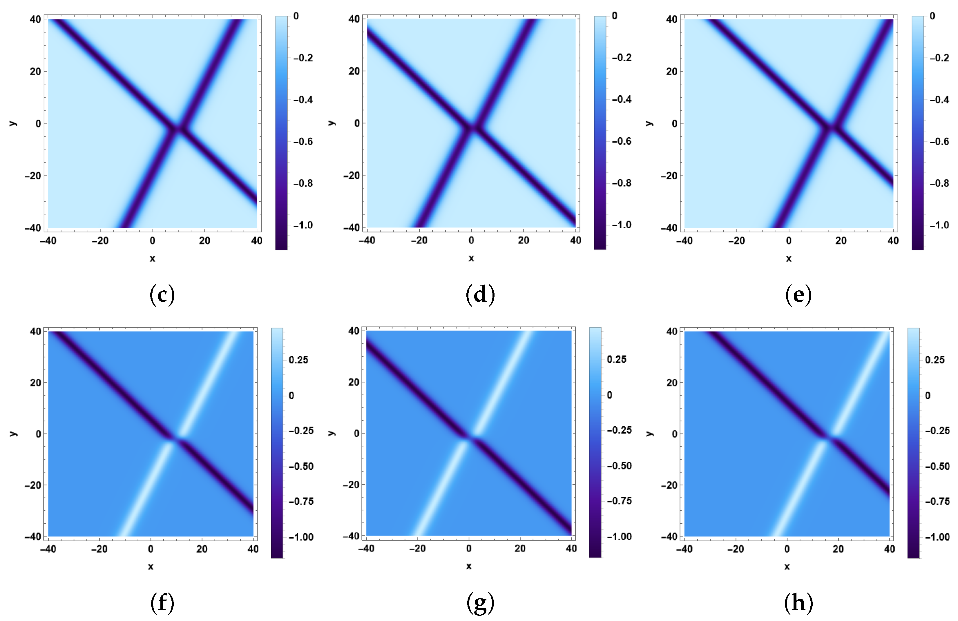
The profiles of two-solitons described by Equation (33) are shown in Figure 2. Figure 2a,b are the 3D plots of $r(x,0,t)$ and $v(x,0,t)$. Figure 2c–h are the density plots of $r(x,y,t_0)$ and $v(x,y,t_0)$ with different values of $t_0$.

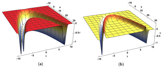
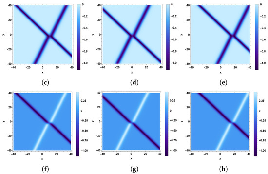
Figure 2. Plots of solutions (33) with the parameters $a_1=-0.8, b_1=0.4, a_2=0.85, b_2=0.9, {\zeta }_1={\zeta }_2=0, \alpha \left(t\right)=t, \beta \left(t\right)=1$, and (a) 3D plots: $r(x,0,t)$, (b) 3D plots: $v(x,0,t)$, (c) $r(x,y,-5)$, (d) $r(x,y,0)$, (e) $r(x,y,5)$, (f) $v(x,y,-5)$, (g) $v(x,y,0)$, (h) $v(x,y,5)$.

The interaction of the two solitons is elastic: The two solitons preserve the shapes after interaction with each other, and there is only a phase difference before and after the collision. In this case, the two-soliton r consistently appears as a dark soliton. If $a_1{b}_1>0$ and $a_2{b}_2>0$, the two-soliton v is also a dark soliton. If $\left(a_1{b}_1\right)\left(a_2{b}_2\right)<0$, v appears as a dark-bright soliton. Finally, if $a_1{b}_1<0$ and $a_2{b}_2<0$, v becomes a bright soliton (see Table 1).

Table 1. Types of the two-soliton v based on different parameter values.

${\mathit{a}}_1{\mathit{b}}_1$	${\mathit{a}}_2{\mathit{b}}_2$	Type
positive	positive	dark soliton
positive	negative	mixed soliton
negative	positive	mixed soliton
negative	negative	bright soliton

4. Lumps and Lump-Solitary Waves

4.1. Lump Solutions

Lump solutions are a special kind of rational solution. Assume that $\varphi$ is defined as a combination of two positive quadratic functions, given by

$$\varphi ={\theta }_1^2+{\theta }_2^2+k,$$

(34)

where ${\theta }_i=a_{i}x+b_{i}y+c_i\left(t\right)$ for $i=1,2$. To ensure that $\varphi >0$, we require $k>0$. By substituting Equation (34) into Equation (22) and simplifying, we find that the parameters satisfy the following relations:

$$\begin{array}{cc}\hfill & c_1\left(t\right)=-a_1\int \alpha \left(t\right)dt+d_1,\hfill \\ \hfill & c_2\left(t\right)=-a_1\int \alpha \left(t\right)dt+d_2,\hfill \\ \hfill & a_1{b}_1+a_2{b}_2=0,\hfill \\ \hfill & C=0,\hfill \end{array}$$

(35)

where $d_1$ and $d_2$ are arbitrary constants. Thus, Equation (34) can be reduced to

$$\varphi =(a_1^2+a_2^2){\left(x-\int \alpha \left(t\right)dt\right)}^2+(b_1^2+b_2^2)y^2+k_0,$$

(36)

where $k_0=k+d_1^2+d_2^2>0$ and $a_1{b}_1+a_2{b}_2=0$.

Based on the transformation given by Equation (19), we obtain the lump solution of Equation (7):

$$u=-12{\displaystyle \frac{(a_1^2+a_2^2)\left(x-\int \alpha \left(t\right)dt\right)}{(a_1^2+a_2^2){(x-\int \alpha \left(t\right)dt)}^2+(b_1^2+b_2^2)y^2+k_0}}.$$

(37)

By substituting Equation (37) into Equation (8), we obtain the following expressions:

$$\begin{array}{cc}\hfill r& =12(a_1^2+a_2^2){\displaystyle \frac{(a_1^2+a_2^2){(x-\int \alpha \left(t\right)dt)}^2-(b_1^2+b_2^2)y^2-k_0}{{\left((a_1^2+a_2^2){(x-\int \alpha \left(t\right)dt)}^2+(b_1^2+b_2^2)y^2+k_0\right)}^2}},\hfill \\ \hfill v& =24{\displaystyle \frac{(a_1^2{b}_2^2+a_2^2{b}_1^2)y(x-\int \alpha \left(t\right)dt)}{{\left((a_1^2+a_2^2){(x-\int \alpha \left(t\right)dt)}^2+(b_1^2+b_2^2)y^2+k_0\right)}^2}}.\hfill \end{array}$$

(38)

Both the single lump solutions r and v are independent of the coefficient $\beta \left(t\right)$, and the variable coefficient $\alpha \left(t\right)$ only affects the velocity of the lump waves. By virtue of the extreme value theory of multi-variable functions, we obtain the amplitude of the lump waves r and v (see Table 2).

Table 2. Maximum and minimum of the single lump solutions (38).

	Maximum/Minimum Value	Extreme Point(s)
Maximum of $\mathit{r}$	$1.5(a_1^2+a_2^2)/k_0$	$(\alpha \left(t\right)\pm \sqrt{3k_0/(a_1^2+a_2^2)},0)$
Minimum of $\mathit{r}$	$-12(a_1^2+a_2^2)/k_0$	$\left(\alpha \right(t),0)$
Maximum of $\mathit{v}$	$3\sqrt{(a_1^2+a_2^2)(b_1^2+b_2^2)}/k_0$	$(\alpha \left(t\right)\pm \sqrt{{\displaystyle \frac{k_0}{2(a_1^2+a_2^2)}}},\pm \sqrt{{\displaystyle \frac{k_0}{2(b_1^2+b_2^2)}}})$
Minimum of $\mathit{v}$	$-3\sqrt{(a_1^2+a_2^2)(b_1^2+b_2^2)}/k_0$	$(\alpha \left(t\right)\pm \sqrt{{\displaystyle \frac{k_0}{2(a_1^2+a_2^2)}}},\mp \sqrt{{\displaystyle \frac{k_0}{2(b_1^2+b_2^2)}}})$

In order to analyze the asymptotic properties of the vector field, we set $\alpha \left(t\right)$ and $\beta \left(t\right)$ to constants, i.e., $\alpha \left(t\right)=\alpha$ and $\beta \left(t\right)=\beta$, and we obtain

$$r\sim {\displaystyle \frac{12}{{\alpha }^2}}{t}^{-2},v\sim {\displaystyle \frac{-24(b_1^2+b_2^2)y}{(a_1^2+a_2^2){\alpha }^3}}{t}^{-3},t\to \infty$$

(39)

As $t\to \pm \infty$, the vector field uniformly approaches a constant background.

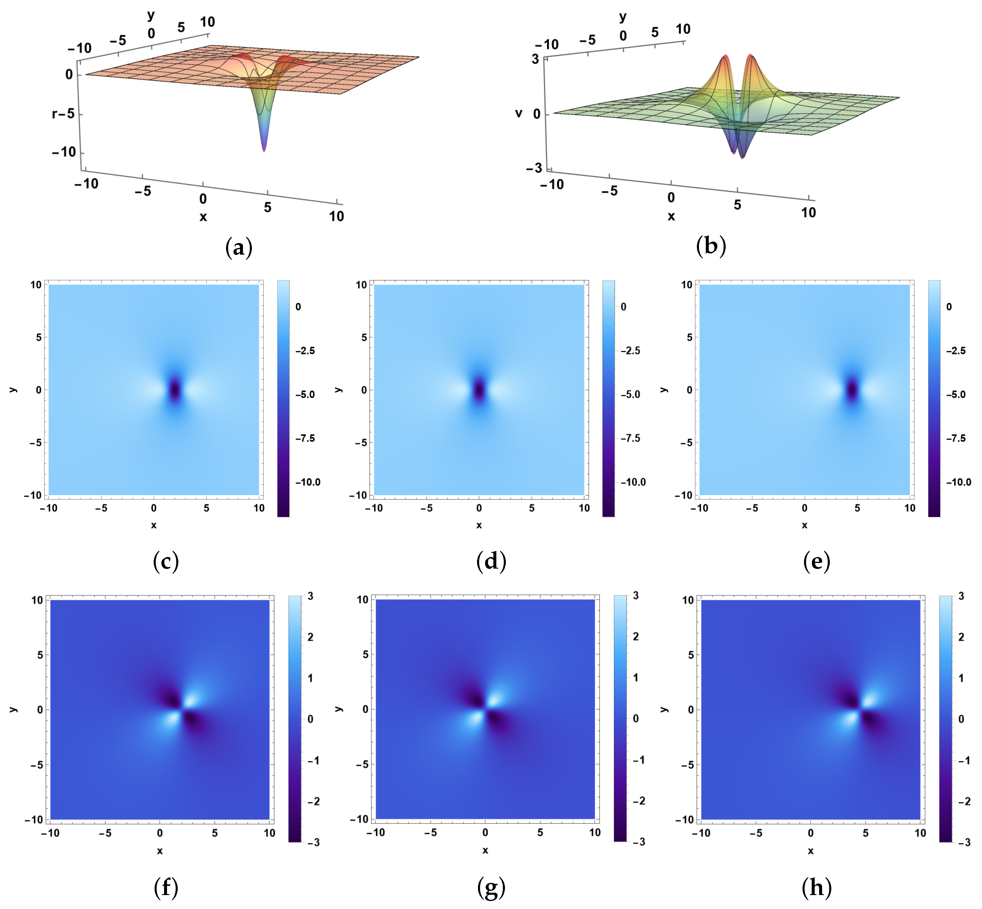
The profiles of single-lump waves described by Equation (38) are shown in Figure 3. Figure 3a,b are the 3D plots of $r(x,y,0)$ and $v(x,y,0)$. Figure 3c–h are the density plots of $r(x,y,t_0)$ and $v(x,y,t_0)$ with different values of $t_0$.

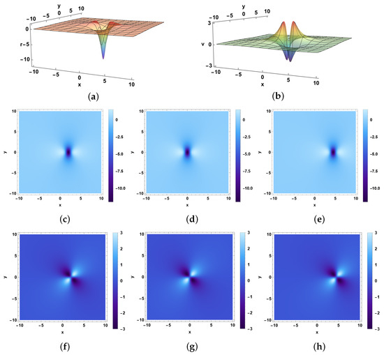
Figure 3. Plots of solutions (38) with the parameters $a_1=1, b_1=1, a_2=-1, b_2=1, k_0=2, \alpha \left(t\right)=t$, and (a) 3D plots: $r(x,y,0)$, (b) 3D plots: $v(x,y,0)$, (c) $r(x,y,-2)$, (d) $r(x,y,0)$, (e) $r(x,y,3)$, (f) $v(x,y,-2)$, (g) $v(x,y,0)$, (h) $v(x,y,3)$.

Both of the two lump waves are completely localized. The lump wave v exhibits a pattern with two high peaks and two deep holes under the plane, while the lump wave r exhibits a pattern with two high peaks and one deep hole. The lump waves r and v have the same velocity of $\alpha \left(t\right)$, and they move along the x-axis with their shapes preserving during the wave propagation.

4.2. Breather Solutions

The m-breather solutions can be derived from the $2m$-soliton solutions. We set ${\eta }_{2n}={\eta }_{2n-1}^{*}$, and the coefficients given in Equation (24) are written as follows:

$$\begin{array}{cc}\hfill a_{2n-1}& =k_n+i{p}_n,a_{2n}=k_n-i{p}_n,\hfill \\ \hfill b_{2n-1}& =l_n+i{q}_n,b_{2n}=l_n-i{q}_n,\hfill \\ \hfill {\zeta }_{2n-1}& ={\zeta }_{2n}=0.\hfill \end{array}$$

(40)

The one-breather solutions of Equation (7) can be generated with the function $\varphi$ as follows:

$$\begin{array}{cc}\hfill & \varphi =1+2e^{R_1}cos{I}_1+{\alpha }_{12}{e}^{2R_1},\hfill \\ \hfill & {\alpha }_{12}=-{\displaystyle \frac{p_1{q}_1}{k_1{l}_1}},\hfill \end{array}$$

(41)

where the real and imaginary parts of ${\eta }_1$ are

$$\begin{array}{cc}\hfill & R_1=\Re \left({\eta }_1\right)=k_{1}x+l_{1}y-\int \left(\beta \left(t\right)k_1(k_1^2-3p_1^2)+\alpha \left(t\right)k_1\right)dt,\hfill \\ \hfill & I_1=\Im \left({\eta }_1\right)=p_{1}x+q_{1}y-\int \left(\beta \left(t\right)p_1(3k_1^2-p_1^2)+\alpha \left(t\right)p_1\right)dt.\hfill \end{array}$$

(42)

Thus, we obtain the breather solution of Equation (7):

$$u=-12e^{R_1}{\displaystyle \frac{k_{1}cos{I}_1-p_{1}sin{I}_1+k_1{\alpha }_{12}{e}^{R_1}}{1+2e^{R_1}cos{I}_1+{\alpha }_{12}{e}^{2R_1}}}.$$

(43)

By substituting Equation (43) into Equation (8), we obtain the following expressions:

$$\begin{array}{cc}\hfill r& =-12e^{R_1}{\displaystyle \frac{(1+{\alpha }_{12}{e}^{2R_1})(k_1^2-p_1^2)cos{I}_1-2(1-{\alpha }_{12}{e}^{2R_1})k_1{p}_{1}sin{I}_1-2(p_1^2+k_1^2{\alpha }_{12})e^{R_1}}{{(1+2e^{R_1}cos{I}_1+{\alpha }_{12}{e}^{2R_1})}^2}},\hfill \\ \hfill v& =-12e^{R_1}{\displaystyle \frac{(1+{\alpha }_{12}{e}^{2R_1})(k_1{l}_1-p_1{q}_1)cos{I}_1-(1-{\alpha }_{12}{e}^{2R_1})(k_1{q}_1+l_1{p}_1)sin{I}_1-2(k_1{q}_1+l_1{p}_1)e^{R_1}}{{(1+2e^{R_1}cos{I}_1+{\alpha }_{12}{e}^{2R_1})}^2}}.\hfill \end{array}$$

(44)

The profiles of breather waves given by Equation (44) are shown in Figure 4. Figure 4a,b are the 3D plots of $r(x,y,0)$ and $v(x,y,0)$. Figure 4c–h are the density plots of $r(x,y,t_0)$ and $v(x,y,t_0)$ with different values of $t_0$.

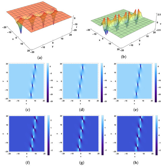
Figure 4. Plots of solutions (44) with the parameters $k_1=-1, p_1=0.6, l_1=0.15, q_1=0.5, \alpha \left(t\right)=\beta \left(t\right)=t$, and (a) 3D plots: $r(x,y,0)$, (b) 3D plots: $v(x,y,0)$, (c) $r(x,y,-4)$, (d) $r(x,y,0)$, (e) $r(x,y,3)$, (f) $v(x,y,-4)$, (g) $v(x,y,0)$, (h) $v(x,y,3)$.

The trajectory of r and v is $R_1=0$. Through computing the period of r and v, we obtain the distance between two adjacent peaks is $\left|{\displaystyle \frac{2\pi \sqrt{k_1^2+l_1^2}}{k_1{q}_1-l_1{p}_1}}\right|$. The variable coefficients $\alpha \left(t\right)$ and $\beta \left(t\right)$ only influence the velocity of the breather waves. The breather waves r and v have the same velocity of

$$\overrightarrow{V}\left(t\right)=\left({\displaystyle \frac{k_1^2}{k_1^2+l_1^2}}\left(\beta \left(t\right)(k_1^2-3p_1^2)+\alpha \left(t\right)\right),{\displaystyle \frac{k_1{l}_1}{k_1^2+l_1^2}}\left(\beta \left(t\right)(k_1^2-3p_1^2)+\alpha \left(t\right)\right)\right).$$

(45)

As time progresses, the breathers propagate parallelly on the $(x,y)$-plane, while their shapes remain unchanged.

4.3. Interaction of Lump Waves and Solitary Waves

In this section, we consider the interaction between lump waves and solitary waves. Assume that $\varphi$ is defined as a combination of two positive quadratic functions and one exponential function, given by

$$\varphi ={\theta }_1^2+{\theta }_2^2+h{e}^{{\theta }_3}+k,$$

(46)

where ${\theta }_i=a_{i}x+b_{i}y+c_i\left(t\right)$ for $i=1,2,3$. To ensure that $\varphi >0$, we require $h>0$ and $k>0$. By substituting Equation (46) into Equation (22) and simplifying, we find that the parameters satisfy the following relations:

$$\begin{array}{cc}\hfill & c_1\left(t\right)=-a_1\int \alpha \left(t\right)dt+d_1,\hfill \\ \hfill & c_2\left(t\right)=-a_1\int \alpha \left(t\right)dt+d_2,\hfill \\ \hfill & c_3\left(t\right)=-\int \left(\beta \left(t\right)a_3^3+\alpha \left(t\right)a_3\right)dt,\hfill \\ \hfill & a_1{b}_1+a_2{b}_2=0,b_3=0,\hfill \\ \hfill & C=0,\hfill \end{array}$$

(47)

where $d_1$ and $d_2$ are arbitrary constants.

Thus, Equation (46) can be reduced to

$$\varphi =(a_1^2+a_2^2){(x-\int \alpha \left(t\right)dt)}^2+(b_1^2+b_2^2)y^2+h{e}^{a_{3}x-\int (\beta \left(t\right)a_3^3+\alpha \left(t\right)a_3)dt}+k_0,$$

(48)

where $k_0=k+d_1^2+d_2^2>0$ and $a_1{b}_1+a_2{b}_2=0$. Based on the transformation given by Equation (19), we obtain the interaction solution of the single-lump and single-soliton solutions of Equation (7):

$$u=-6{\displaystyle \frac{a_{3}h{e}^{a_{3}x-\int (\beta \left(t\right)a_3^3+\alpha \left(t\right)a_3)dt}+2(a_1^2+a_2^2)(x-\int \alpha \left(t\right)dt)}{(a_1^2+a_2^2){(x-\int \alpha \left(t\right)dt)}^2+(b_1^2+b_2^2)y^2+h{e}^{a_{3}x-\int (\beta \left(t\right)a_3^3+\alpha \left(t\right)a_3)dt}+k_0}}.$$

(49)

By substituting Equation (49) into Equation (8), we obtain the following expressions:

$$\begin{array}{cc}\hfill r& =6{\displaystyle \frac{2{(a_1^2+a_2^2)}^2{z}_1^2-(2a_1^2+2a_2^2+a_3^{2}h{e}^{a_3{z}_2})(k_0+(b_1^2+b_2^2)y^2)-(a_1^2+a_2^2)h{e}^{a_3{z}_2}(a_3^2{z}_1^2-4a_3{z}_1+2)}{{\left((a_1^2+a_2^2)z_1^2+(b_1^2+b_2^2)y^2+h{e}^{a_3{z}_2}+k_0\right)}^2}},\hfill \\ \hfill v& =12(b_1^2+b_2^2)y{\displaystyle \frac{a_{3}h{e}^{a_3{z}_2}+2(a_1^2+a_2^2)z_1}{{\left((a_1^2+a_2^2)z_1^2+(b_1^2+b_2^2)y^2+h{e}^{a_3{z}_2}+k_0\right)}^2}},\hfill \end{array}$$

(50)

where $z_1=x-\int \alpha \left(t\right)dt$ and $z_2=x-\int (\beta \left(t\right)a_3^2+\alpha \left(t\right))dt$.

In order to analyze the asymptotic properties of the vector field, we set $\alpha \left(t\right)$ and $\beta \left(t\right)$ to constants, i.e., $\alpha \left(t\right)=\alpha$ and $\beta \left(t\right)=\beta$. We find that $z_1$ has a velocity of $\alpha$, while $z_2$ has a velocity of $\alpha +a_3^2\beta$. Without loss of generality, we assume $\alpha ,\beta ,a_3>0$. In the coordinate system of the lump wave, we fix $z_1$, resulting in:

$$\begin{array}{cc}\hfill & \varphi \sim h{e}^{a_3{z}_2}+O\left(t^2\right),t\to -\infty ,\hfill \\ \hfill & \varphi \sim (a_1^2+a_2^2)z_1^2+(b_1^2+b_2^2)y^2+k_0,t\to +\infty ,\hfill \end{array}$$

(51)

where $O\left(t^2\right)$ represents a quantity that is infinitely smaller than $e^{a_3{z}_2}$ as $t\to -\infty$.

Therefore, we find that as $t\to -\infty$, the lump-solitary wave r becomes a single-solitary wave and v returns to a zero background. Conversely, the lump-solitary waves r and v evolve into single-lump waves as $t\to +\infty$.

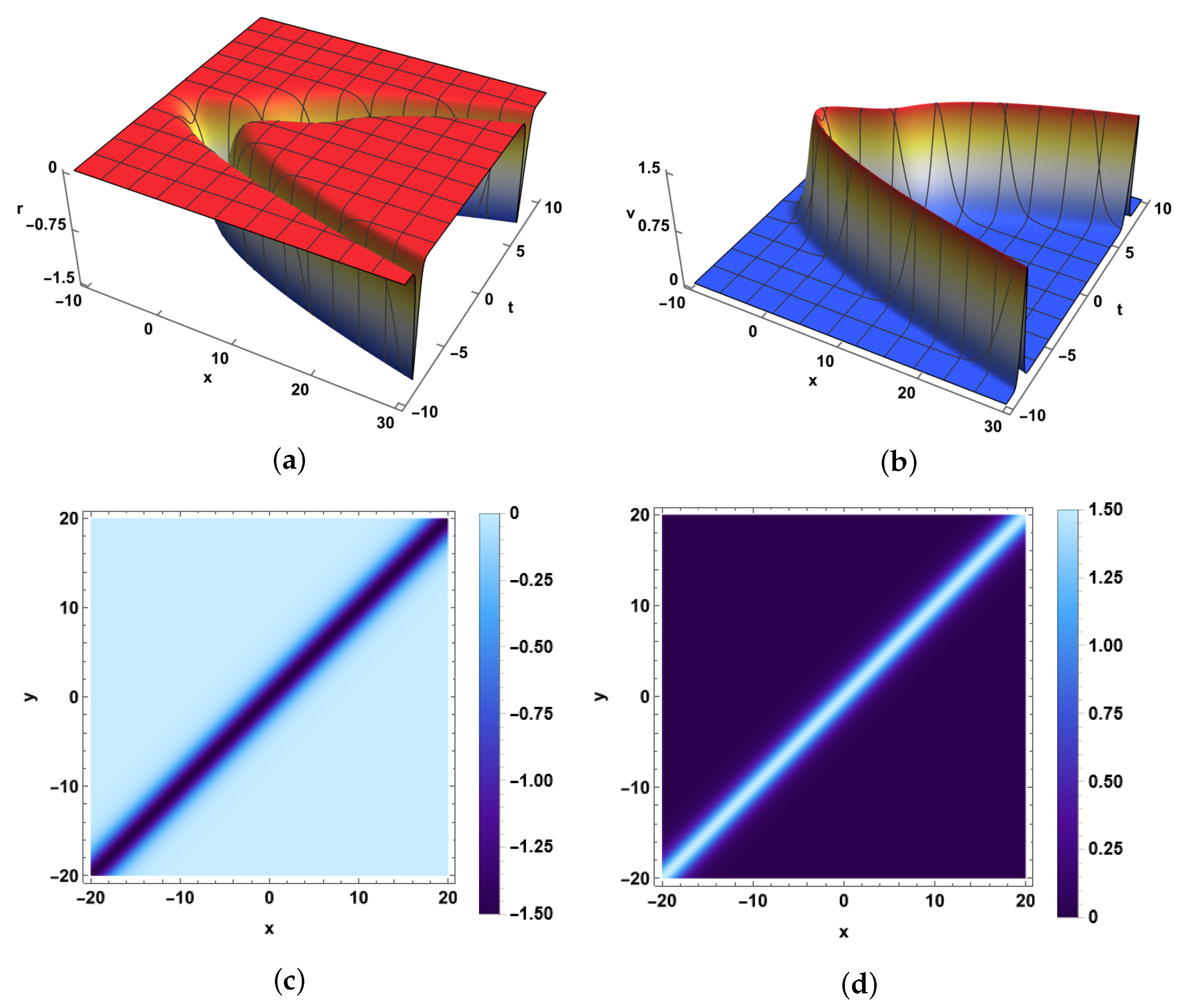
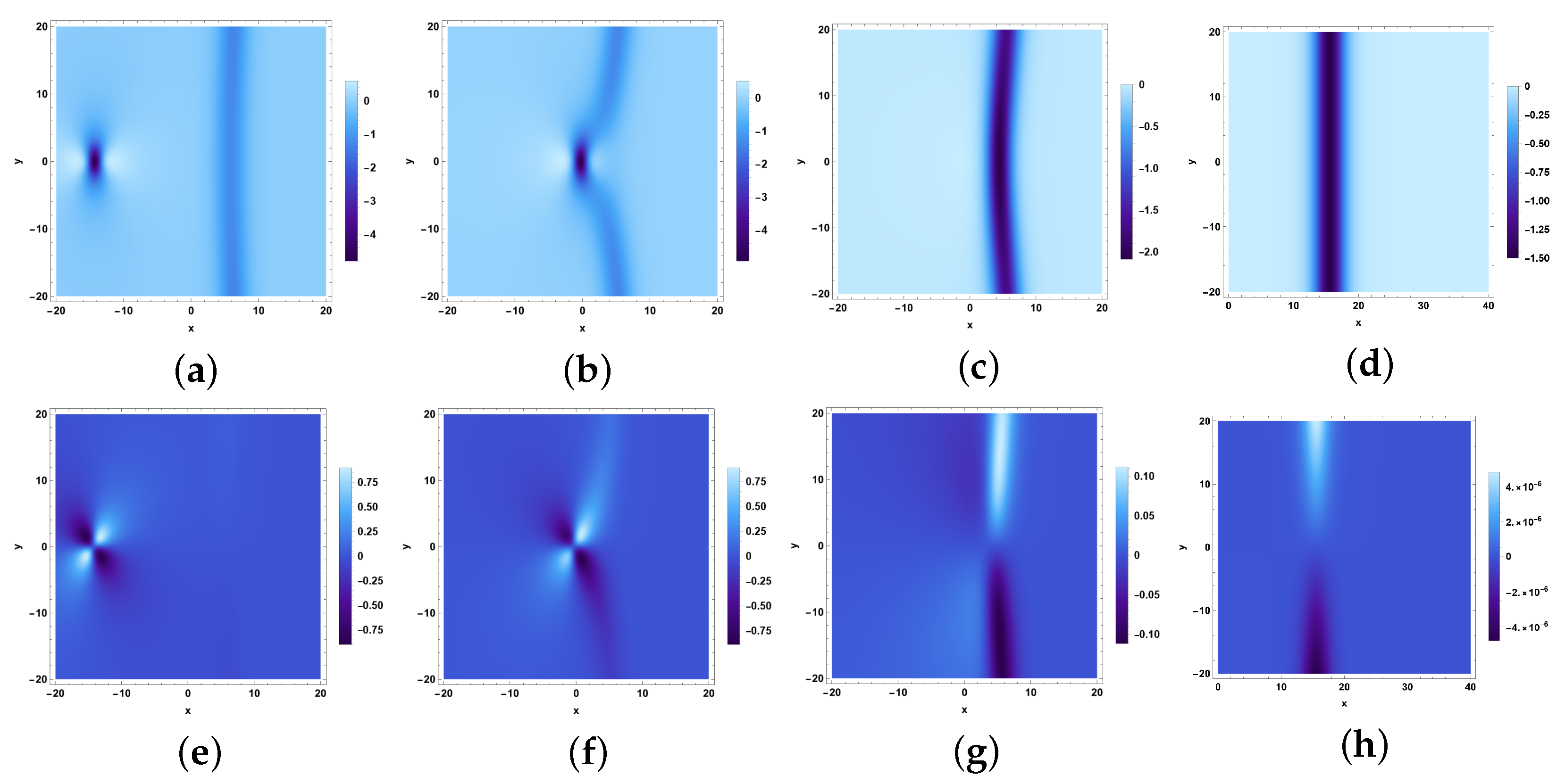
The profiles of lump-solitary waves described by Equation (50) are shown in Figure 5 and Figure 6. Figure 5a,b are the 3D plots of $r(x,y,0)$ and $v(x,y,0)$. The variable coefficients $\alpha \left(t\right)$ and $\beta \left(t\right)$ influence the velocities of the lump waves and the solitary waves. The interaction of the two waves presents different situations for different $\alpha \left(t\right)$ and $\beta \left(t\right)$. We primarily focus on the interaction phenomena involving the emergence of the lump wave from the solitary wave, as well as the collisions between the lump wave and the solitary wave.

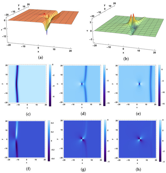
Figure 5. Plots of solutions (50) with the parameters $a_1=1, b_1=1, a_2=-1, b_2=1, a_3=2, k_0=1.5, h=0.5e^{-2}, \alpha \left(t\right)=t^2, \beta \left(t\right)=1$, and (a) 3D plots: $r(x,y,0)$, (b) 3D plots: $v(x,y,0)$, (c) $r(x,y,-2.5)$, (d) $r(x,y,0)$, (e) $r(x,y,2)$, (f) $v(x,y,-2.5)$, (g) $v(x,y,0)$, (h) $v(x,y,2)$.

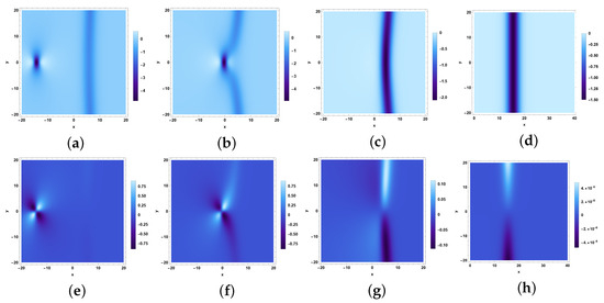
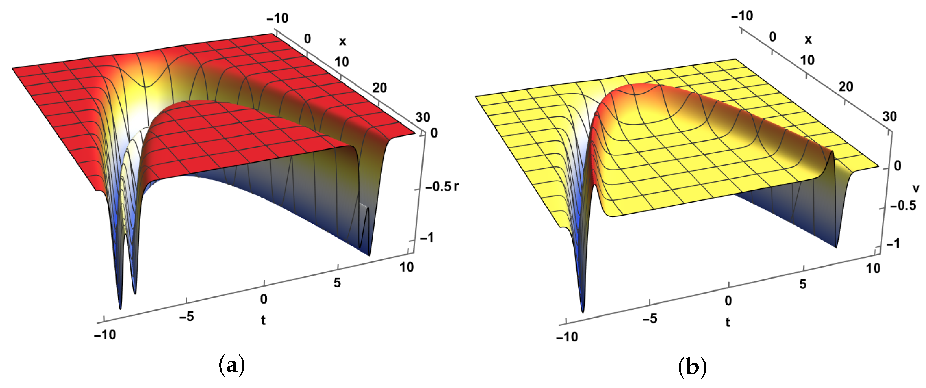
Figure 6. Plots of solutions (50) with the parameters $a_1=0.8, b_1=-0.3, a_2=0.4, b_2=0.6, a_3=1, k_0=2, h=1, \alpha \left(t\right)=t^2, \beta \left(t\right)=-t^2$, and (a) $r(x,y,-3.5)$, (b) $r(x,y,0)$, (c) $r(x,y,3.5)$, (d) $r(x,y,20)$ (e) $v(x,y,-3.5)$, (f) $v(x,y,0)$, (g) $v(x,y,3.5)$, (h) $v(x,y,20)$.

As shown in Figure 5, it is evident that the lump wave emerges from the stripe soliton (see Figure 5c,f). As $t\to 0$, the lump wave separates from the solitary wave, with part of the soliton’s energy transferring into the lump wave (see Figure 5d,g). As time increases, the lump wave moves away from the soliton (see Figure 5e,h). The lump wave is semi-localized in time, indicating that it exhibits properties characteristic of rogue waves.

Conversely, as shown in Figure 6, when the soliton’s velocity is set to zero, the lump wave travels toward the soliton (see Figure 6a,e). As $t\to 0$, the solitary wave is attracted to the lump wave, gradually transferring energy from the lump wave to the soliton (see Figure 6b,f). Eventually, the lump wave is completely absorbed by the stripe soliton, merging the two types of waves into one, with the soliton gaining the kinetic energy of the lump wave (see Figure 6c,g). As time increases, r travels as a soliton, while v gradually returns to a zero background (see Figure 6d,h).

5. Conclusions and Discussion

In this paper, the (2+1)-D eSWW equation with variable coefficients was systematically analyzed. The Painlevé integrable condition of Equation (7) was investigated through Painlevé analysis. Utilizing Hirota’s bilinear method, we have discovered soliton solutions, lump solutions, breather solutions, and interaction solutions for the vc-eSWW equation. By reducing the equations to a pair of coupled equations, we obtained the physical properties of lump waves: lumps can emerge from solitary waves and are semi-localized in time.

Notably, we have explored the interaction between lump waves and solitary waves through the exact solutions of this equation. First, the lump wave can emerge from a single soliton, after which the two waves separate from each other. Second, the lump wave cannot travel across a solitary wave and will be absorbed by it upon meeting. Third, after the solitary wave swallows the lump wave, the two components of the vector field exhibit entirely different long-term asymptotic behaviors: the x-component remains as a solitary wave, while the y-component returns to a zero background.

The binary Darboux transformation also serves as an efficient tool for constructing lump solutions, which may inspire our related work [36]. Additionally, deriving multi-lump solutions and higher-order lump solutions of Equation (7) will be the focus of our future research, including a discussion on the Lax integrability of the equation.

References

- Mei, C.C.; Stiassnie, M.; Yue, D. Theory and Applications of Ocean Surface Waves; World Scientific: Singapore, 2005. [Google Scholar]
- Izadi, M.; Yadav, S.K.; Methi, G. Two efficient numerical techniques for solutions of fractional shallow water equation. Partial Differ. Equ. Appl. Math. 2024, 9, 100619. [Google Scholar] [CrossRef]
- Hossain, M.D.; Alam, M.K.; Akbar, M.A. Abundant wave solutions of the Boussinesq equation and the (2+1)-dimensional extended shallow water wave equation. Ocean Eng. 2018, 165, 69–76. [Google Scholar] [CrossRef]
- Li, D.F.; Dong, J. A robust hybrid unstaggered central and Godunov-type scheme for Saint-Venant-Exner equations with wet/dry fronts. Comput. Fluids 2022, 235, 105284. [Google Scholar] [CrossRef]
- Magdalena, I.; Imawan, R.; Nugroho, M.A. Numerical investigation for water flow in an irregular channel using Saint-Venant equations. J. King Saud Univ. Sci. 2024, 36, 103237. [Google Scholar] [CrossRef]
- Korteweg, D.J.; de Vries, G. On the change of form of long waves advancing in a rectangular canal, and on a new type of long stationary waves. Philos. Mag. 1895, 39, 422–443. [Google Scholar] [CrossRef]
- Ablowitz, M.J.; Clarkson, P.A. Solitons, Nonlinear Evolution Equations and Inverse Scattering; Cambridge University Press: Cambridge, UK, 1991. [Google Scholar]
- Boiti, M.; Leon, J.; Manna, M.; Pempinelli, F. On the spectral transform of a Korteweg-de Vries equation in two spatial dimensions. Inverse Probl. 1986, 2, 271. [Google Scholar] [CrossRef]
- Roshid, H.; Ma, W.X. Dynamics of mixed lump-solitary waves of an extended (2+1)-dimensional shallow water wave model. Phys. Lett. A 2018, 382, 3262–3268. [Google Scholar] [CrossRef]
- Yang, J.K. Nonlinear Waves in Integrable and Nonintegrable Systems; Society for Industrial and Applied Mathematics: Philadelphia, PA, USA, 2010. [Google Scholar]
- Konno, K.; Wadati, M. Simple derivation of Bäcklund transformation from Riccati form of inverse method. Prog. Theor. Phys. 1975, 53, 1652–1656. [Google Scholar] [CrossRef]
- Weiss, J. The Painlevé property for partial differential equations. II: Bäcklund transformation, Lax pairs, and the Schwarzian derivative. J. Math. Phys. 1983, 24, 1405–1413. [Google Scholar] [CrossRef]
- Li, X.N.; Wei, G.M.; Liang, Y.Q. Painlevé analysis and new analytic solutions for variable-coefficient Kadomtsev-Petviashvili equation with symbolic computation. Appl. Math. Comput. 2010, 216, 3568–3577. [Google Scholar] [CrossRef]
- Wadati, M.; Sanuki, H.; Konno, K. Relationships among inverse method, Bäcklund transformation and an infinite number of conservation laws. Prog. Theor. Phys. 1975, 53, 419–436. [Google Scholar] [CrossRef]
- Rogers, C.; Schief, W. Bäcklund and Darboux Transformations: Geometry and Modern Applications in Soliton Theory; Cambridge University Press: Cambridge, UK, 2002. [Google Scholar]
- Hirota, R. Exact solution of the Korteweg-de Vries equation for multiple collisions of solitons. Phys. Rev. Lett. 1971, 27, 1192–1194. [Google Scholar] [CrossRef]
- Yang, X.Y.; Zhang, Z.; Wang, Z. Degenerate lump wave solutions of the Mel’nikov equation. Nonlinear Dyn. 2023, 111, 1553–1563. [Google Scholar] [CrossRef]
- Nuruzzaman, M.; Kumar, D. Lumps with their some interactions and breathers to an integrable (2+1)-dimensional Boussinesq equation in shallow water. Results Phys. 2022, 38, 105642. [Google Scholar] [CrossRef]
- Matveev, V.B.; Sall, M.A. Scattering of solitons in the formalism of the Darboux transform. J. Sov. Math. 1986, 34, 1983–1987. [Google Scholar] [CrossRef]
- Chen, S.Y.; Yan, Z.Y. The Hirota equation: Darboux transform of the Riemann-Hilbert problem and higher-order rogue waves. Appl. Math. Lett. 2019, 95, 65–71. [Google Scholar] [CrossRef]
- Bluman, G.W.; Cheviakov, A.F.; Anco, S.C. Applications of Symmetry Methods to Partial Differential Equations; Springer: Berlin/Heidelberg, Germany, 2010. [Google Scholar]
- Clarkson, P.A. New similarity solutions for the modified Boussinesq equation. J. Phys. A Math. Gen. 1989, 22, 2355. [Google Scholar] [CrossRef]
- Manikandan, K.; Muruganandam, P.; Senthilvelan, M.; Lakshmanan, M. Manipulating localized matter waves in multicomponent Bose-Einstein condensates. Phys. Rev. E 2016, 93, 032212. [Google Scholar] [CrossRef] [PubMed]
- Manigandan, M.; Manikandan, K.; Muniyappan, A.; Jakeer, S.; Sirisubtawee, S. Deformation of inhomogeneous vector optical rogue waves in the variable coefficients coupled cubic–quintic nonlinear Schrödinger equations with self-steepening. Eur. Phys. J. Plus 2024, 139, 405. [Google Scholar] [CrossRef]
- Ablowitz, M.J.; Segur, H. Solitons and the Inverse Scattering Transform; Society for Industrial and Applied Mathematics: Philadelphia, PA, USA, 1981. [Google Scholar]
- Cao, Y.L.; Cheng, Y.; Malomed, B.A.; He, J.S. Rogue waves and lumps on the nonzero background in the PT symmetric nonlocal Maccari system. Stud. Appl. Math. 2021, 147, 694–723. [Google Scholar] [CrossRef]
- Dawod, L.A.; Lakestani, M.; Manafian, J. Breather wave solutions for the (3+1)-D generalized shallow water wave equation with variable coefficients. Qual. Theory Dyn. Syst. 2023, 22, 127. [Google Scholar] [CrossRef]
- Yang, X.Y.; Wang, Z.; Zhang, Z. Generation of anomalously scattered lumps via lump chains degeneration within the Mel’nikov equation. Nonlinear Dyn. 2023, 111, 15293–15307. [Google Scholar] [CrossRef]
- Li, W.; Li, B. Construction of degenerate lump solutions for (2+1)-dimensional Yu-Toda-Sasa-Fukuyama equation. Chaos Solition Fract. 2024, 180, 114572. [Google Scholar] [CrossRef]
- Yuan, F.; He, J.S.; Cheng, Y. Exact solutions of a (2+1)-dimensional extended shallow water wave equation. Chin. Phys. B 2019, 28, 100202. [Google Scholar] [CrossRef]
- Ismael, H.F.; Seadawy, A.; Bulut, H. Multiple soliton, fusion, breather, lump, mixed kink-lump and periodic solutions to the extended shallow water wave model in (2+1)-dimensions. Mod. Phys. Lett. B 2021, 35, 2150138. [Google Scholar] [CrossRef]
- He, L.; Zhang, J.; Zhao, Z. Multiple M-lump and interaction solutions of a (2+1)-dimensional extended shallow water wave equation. Eur. Phys. J. Plus 2021, 136, 192. [Google Scholar] [CrossRef]
- Adeyemo, O.D.; Khalique, C.M. Stability analysis, symmetry solutions and conserved currents of a two-dimensional extended shallow water wave equation of fluid mechanics. Partial Differ. Equ. Appl. Math. 2021, 4, 100134. [Google Scholar] [CrossRef]
- Wei, G.; Gao, Y.; Hu, W.; Zhang, C. Painlevé analysis, auto-Bäcklund transformation and new analytic solutions for a generalized variable-coefficient Korteweg-de Vries (KdV) equation. Eur. Phys. J. B 2006, 53, 343–350. [Google Scholar] [CrossRef]
- Weiss, J.; Tabor, M.; Carnevale, G. The Painlevé property for partial differential equations. J. Math. Phys. 1983, 24, 1405–1413. [Google Scholar] [CrossRef]
- Guo, L.J.; Chen, L.; Mihalache, D.; He, J.S. Dynamics of soliton interaction solutions of the Davey-Stewartson I equation. Phys. Rev. E 2022, 105, 014218. [Google Scholar] [CrossRef]
Disclaimer/Publisher’s Note: The statements, opinions and data contained in all publications are solely those of the individual author(s) and contributor(s) and not of MDPI and/or the editor(s). MDPI and/or the editor(s) disclaim responsibility for any injury to people or property resulting from any ideas, methods, instructions or products referred to in the content. |
© 2024 by the authors. Licensee MDPI, Basel, Switzerland. This article is an open access article distributed under the terms and conditions of the Creative Commons Attribution (CC BY) license (https://creativecommons.org/licenses/by/4.0/).