Reliabilityand Sensitivity Analysis of Wireless Sensor Network Using a Continuous-Time Markov Process

Abstract

A remarkably high growth has been observed in the uses of wireless sensor networks (WSNs), due to their momentous potential in various applications, namely the health sector, smart agriculture, safety systems, environmental monitoring, military operations, and many more. It is quite important that a WSN must have high reliability along with the least MTTF. This paper introduces a continuous-time Markov process, which is a special case of stochastic process, based on modeling of a wireless sensor network for analyzing the various reliability indices of the same. The modeling has been conducted by considering the different components, including the sensing unit, transceiver, microcontroller, power supply, standby power supply unit, and their failures/repairs, which may occur during their functioning. The study uncovered different important assessment parameters like reliability, components-wise reliability, MTTF, and sensitivity analysis. The critical components of a WSN are identified by incorporating the concept of sensitivity analysis. The outcomes emphasize that the proposed model will be ideal for understanding different reliability indices of WSNs and guiding researchers and potential users in developing a more robust wireless sensor network system.

1. Introduction

A wireless sensor network (WSN) is a collection of spatially distributed independent sensors that communicate wirelessly to fetch data about any physical and environmental condition/activity. WSN systems were introduced in the 19th century and have become a critical technology across various fields. Their growing importance attracts researchers, scholars, and scientists from different domains. In recent decades, the growth of wireless connectivity has been exponential, driven by its potential applications in environmental monitoring, healthcare, medical sciences, military surveillance, agriculture, industry, and smart cities. Moreover, WSNs have become the framework of many IOT applications and act as the backbone in connecting various devices and enabling seamless communication. Khandris [1] presented remarkable advantages of WSNs and explained how rapidly evolving technological domains need WSNs. Baduge et al. [2] extensively investigated applications of AI in Industry 4.0 and highlighted the vital role of wireless sensor networks in accelerating progress in various fields. Adu-Manu et al. [3] explored sensor network architecture that can be used for various applications and also discussed advances in WSNs with machine learning and the IOT. Chowdhury et al. [4] explained various technologies that will drive 6G communications and presented possible applications and the technologies to be deployed for 6G communications. Microcontroller unit-based wireless sensor nodes were investigated by Khalifeh et al. [5], who also reviewed the progress made by industry and academia in designing wireless sensor nodes to avoid redundancy. Analysis conducted by Lanzolla et al. [6] demonstrated the significant progress and potential of WSNs in environmental monitoring.

Many researchers and engineers have contributed towards the methodology, which improves the performance of various industrial systems by identifying numerous parameters that affect the performance of the overall system [7,8,9]. Consistent and accurate data transmission in complex industrial applications is essential for efficient and safe operations. Therefore, ensuring the reliability of WSNs is vital to maintain the system’s integrity and prevent accidents. In critical applications, network disruption can lead to severe consequences, including safety risks and significant financial losses. However, the effectiveness of WSNs and their performance in different environmental conditions are highly dependent on some crucial parameters such as reliability, availability, and sensitivity. Arjannikov et al. [10] developed a model for assessing failure and repair rates in network systems using Markov chains with various preliminary experiments and case studies for demonstrating their application. Oreku [11] studied WSN reliability, which is used in environment security services where security is of utmost concern for the end users. Mishra and Dash [12] proposed a model to compute reliability under different failure models and environmental conditions. Authors also ensured that the proposed method, to evaluate the reliability of WSNs, is more accurate, even though it uses a lesser number of states. Shrestha et al. [13] presented a method to evaluate the reliability of WSNs by integrating sensing coverage with network connectivity and impact of common cause failure. This approach is illustrated with a hierarchical clustered WSN. Kabashkin and Kundler [14] studied the reliability of sensor nodes in wireless sensor networks within a cyber-physical system. They demonstrated that a sensor node’s reliability is affected by its monitoring strategy, with reliability following an unimodal function relative to the test period. The dependability of WSNs in an industrial environment through fault tree analysis has been conducted by Silva et al. [15]. The authors examined dependability issues, estimated redundancy needs, and suggested a network design. The study revealed that the overall reliability of a WSN is affected by routing protocol, density of nodes, and distance between nodes [16]. Catelani et al. [17] highlighted the impact of redundancy and node deployment on the reliability of WSNs in smart farming by comparing series RBD and territory-based FTA, which signify that hybrid RBD is the most reliable model. Jung and Choi [18] introduced a Markov model for quantitatively analyzing the reliability of satellite communication networks that utilize onboard processing (OBP) satellites. The results showed that network reliability is significantly affected by both satellite channels and onboard processing (OBP) structures. Markov processes have been used to design a P2P network to evaluate different reliability characteristics for the same. The author also emphasizes the components whose failure rates have to be controlled in order to achieve high reliability for the P2P network [19]. Ram et al. [20] studied IoT-based FAS to understand the nature of different performance measures; here, authors also performed sensitivity analysis for the same. Singh et al. [21] studied a $(k,n,G)$ system, with warm standby redundancy and sudden server failure, and found the reliability measures of it. Kumar and Kumar [22] analyzed the communication system’s reliability using the Markov mathematical model. The authors also concluded that communication channel failures affect the system’s reliability the most. Bisht et al. [23] extensively investigated network reliability by focusing on the importance of the network components using measures like Birnbaum importance. The study contributes to the improvement of network performance, which is crucial for architects and engineers. Shunqi et al. [24] introduced a continuous-time Bayesian network for analyzing the reliability of a dynamic wireless communication network. Poonia [25] conducted a reliability and sensitivity analysis of a computer lab. IOT applications are evolving rapidly, and there is a need to address the complexity of these systems. Xing [26] proposed a survey on existing models, focusing on their shortcomings and the need for a reliable model to address the ongoing revolutionary transformation. Kumar and Kumar [27] examined an IOT-based sensor system that is used in smart garbage collection bins. Using the Markov mathematical model, they identified the most vulnerable sensors and proposed a preventative maintenance strategy. Xing et al. [28] presented a behavior-driven reliability modeling method for a complex WSN-based smart system. The method’s effectiveness was illustrated through a case study on smart homes. The reliability measures of a mobile communication system (MCS) are investigated by Choudhary et al. [29]. A numerical-based case study has been performed to showcase the model graphically, as MCS has become a crucial need worldwide. Wang et al. [30] examined the sensitivity analysis of wireless sensor networks concerning infrastructure communication reliability. Chakraborty et al. [31] addressed the reliability of mobile wireless sensor networks with multiple state nodes. A Monte Carlo Markov chain simulation is proposed for evaluating coverage-oriented reliability. Gupta et al. [32] estimated the availability of a steam turbine power plant. The key challenges were also discussed in the study.

In spite of substantial research in the field of wireless sensor networks, the mathematical modeling of a wireless sensor network through the interconnection of its different components and their cumulative as well as individual effects on overall performance has not been considered, which is necessary for more accurate and effective evaluation. So, here, the author developed a state-based mathematical model for a wireless sensor network, through a continuous-time Markov process, to fill this research gap, which is a significant contribution of this work in the field of reliability analysis of a wireless sensor network. Hence, the purpose of this research is to evaluate the critical aspects of WSN performance such as reliability, component-wise reliability, MTTF, and sensitivity assessment and provide a more robust and reliable system for the evolving technological landscape. A WSN plays a crucial role in various fields, some of which are shown in the Figure 1.

2. Materials and Methods

Reliability of any complex system is always crucial when one wants to optimize its performance. Various reliability indices can further be used for the planning of potential preventive, corrective, and maintenance actions and to maintain the system’s ability for trouble-free operation. Many methods, including fault tree analysis, maximum likelihood estimator, fuzzy membership function, etc., have been used in past to understand the behavior of reliability and related indices. The Markov decision process is also one of such tools that can be used to model an industrial/networking system to understand its various performance measures. During operation, a system can be in any one of these possible states: perfectly working, working with less efficiency (also known as degraded state), and failed state, depending on which components are working perfectly, which are working in a degraded state, and which are components in failed state. More clarity for the system’s reliability can be gathered if it is modeled through the various instances of subsystem failures as well as subsequent repairs. The Markov decision process is a stochastic process through which one can model the different states and transition between them on the basis of different failure/repair rates of the subsystems of a system. The Markov process is introduced by the mathematician “Andrei A, Markov” in early 1900. It is one of the most important processes out of all stochastic process, due to its use and simplicity. A stochastic process is a collection of random variables $Y_t$ defined over some indexed set T. Then, with full generality, it is assumed that for every n, the distribution of $Y_{n+1}$ depends on the whole history $(Y_0=i_0,Y_1=i_1···,Y_n=i_n)$. In contrast, the Markov process asserts that the distribution of $Y_{n+1}$ depends only on the current state $Y_n=i_n$, not on the whole history. Formally, the process $Y_n$ is called a Markov process if for each n and every $i_0,i_1,...,i_n$ and $j\in N$ [33],

$$P[Y_{n+1}=j\mid Y_0=i_0,Y_1=i_1,...,Y_n=i_n]=P[Y_{n+1}=j\mid Y_n=i_n]$$

(1)

The Markov process can be used to model real time problems, per the index variable t. There are two possibilities for t, discrete and continuous. In these cases, the discrete-time Markov process and continuous-time Markov process can be used, respectively. In continuous-time Markov processes, the conditional probability of the future state at time $(t+s)$, given the present state at s and all past states, depends only on the present state and is independent of the past states [34].

$$P[Y_{t+s}=j\mid Y_s=i,Y_u=k,0\le u\le s]=P[Y_{t+s}=j\mid Y_s=i]=P_{ij}\left(t\right)$$

(2)

Here, $P_{ij}\left(t\right)$ represents the transition state probability from the $ith$ state to the $jth$ state. Also, one can understand it as the probability that the Markov process, which is presently in state i, will be in state j after some time t. Further, Equation (2) can be generalized as

$$P_{ij}(t+S)=\sum _{k}P[Y_{t+s}=j,Y_t=k\mid Y_0=i]$$

$$=\sum _k{\displaystyle \frac{P[Y_0=i,Y_t=k,Y_{t+s}=j]}{P[Y_0=i]}}$$

$$=\sum _k{\displaystyle \frac{P[Y_0=i,Y_t=k]}{P[Y_0=i]}}\ast {\displaystyle \frac{P[Y_0=i,Y_t=k,Y_{t+s}=j]}{P[Y_0=i,Y_t=k]}}$$

$$=\sum _{k}P[Y_t=k\mid Y_0=i]\ast P[Y_{t+s}=j\mid Y_0=i,Y_t=k]$$

$$=\sum _{k}P[Y_t=k\mid Y_0=i]\ast P[Y_{t+s}=j\mid Y_t=k]$$

$$=\sum _k{P}_{ik}\left(t\right)P_{kj}\left(s\right)$$

(3)

Equation (3) is known as Chapman–Kolmogorov equations for the continuous-time Markov process. Using the concept of the continuous-time and discrete state space Markov process, along with different failures and repairs that occur during the operation, the author modeled a wireless sensor network (WSN) and obtained the different reliability indices of it. The reliability-based modeling of a WSN through the Markov decision process (MDP) has not been conducted so far, which make this work novel. The obtained measure gives a clear understanding about the performance of the WSN, which will be quite helpful for the management/maintenance team for future operations and extension planing.

2.1. Wireless Sensor Network Description

A WSN comprises ‘nodes’, ranging from a few to hundreds or thousands, where each node connects to other sensors. Each node consists of several parts: a sensing unit, a processing unit, a communication unit, and a power unit (Figure 2).

The sensing unit includes the sensors themselves, which capture environmental data. These data are then processed locally by the processing unit, consisting of a microcontroller or microprocessor, an electronic circuit for interacting with the sensors, and an energy source.

Batteries, or an embedded energy harvesting system, typically power the power unit.

2.2. Nomanculture

The below

Table 1. Nomenclature.

Notation	Description
$t/s$	Time variable/frequency variable
$P_i$(t)	Probability of the system being in the ith state
${\overline{P}}_i$(t)	Represents Laplace transformation of $P_i$(t)
$P_i$ (x,t)	Probability of the failed system being in the ith state
${\overline{P}}_i$(x,s)	Represents Laplace transformation of $P_i$(x,t)
${\lambda }_{su}$/${\lambda }_{ts}$/${\lambda }_m$/${\lambda }_p$/${\lambda }_{ps}$	Represents the failure rate of the sensing unit/transceiver/microcontroller/power supply/standby power supply
${\mu }_{su}$/${\mu }_{ts}$/${\mu }_m$/${\mu }_p$/${\mu }_{ps}$	Represents the repair rate of the sensing unit/transceiver/microcontroller/power supply/standby power supply
${\mu }_{pm}$/${\mu }_{msu}$/${\mu }_{mts}$	Represents repair rate of the power supply and microcontroller/microcontroller and sensing unit/microcontroller and transreceiver
${\mu }_{tsp}$/ ${\mu }_{psp}$/${\mu }_{sup}$	Represents simultaneous repair rate of the trans receiver and power supply/power supply and standby power supply/sensing unit and power supply
${\mu }_{pspm}$/${\mu }_{sump}$/${\mu }_{tsmp}$	Represents repair rate of power supply, standby power supply, and microcontroller/sensing unit, microcontroller, and power supply/transreceiver, microcontroller, and power supply

and

Table 2. Different states’ probability descriptions.

State Probability	Description
$P_0$ (t)	Represents the good state of the system i.e., a state in which and all the components of the WSN are in good working condition
$P_1$ (x,t)	Represents the failed state of the system due to the failure of the sensing unit
$P_2$ (x,t)	Represents the failed state of the system due to the failure of the trans receiver
$P_3$ (t)	Represents the degraded state of the system due to the failure of the one microcontroller
$P_4$ (x,t)	Represents the failed state of the system due to the failure of the both microcontrollers
$P_5$ (t)	Represents that the system is in a degraded state due to the failure of the main power supply
$P_6$ (x,t)	Represents the failed state of the system due to the failure of both the main power supply and standby power supply
$P_7$ (x,t)	Represents the failed state of the system due to the failure of the trans receiver after the failure of the main power supply
$P_8$ (x,t)	Represents the failed state of the system due to the failure of the sensing unit after the failure of the main power supply
$P_9$ (t)	Represents the degraded state of the system after the failure of the main power supply and one microcontroller
$P_{10}$ (x,t)	Represents the failed state of the system due to the failure of both the microcontroller and main power supply
$P_{11}$ (x,t)	Represents the failed state of the system due to the failure of the main power supply, standby power supply, and microcontroller
$P_{12}$ (x,t)	Represents the failed state of the system due to the failure of the sensing unit after the failure of the one microcontroller and main power supply
$P_{13}$ (x,t)	Represents the failed state of the system due to the failure of the trans receiver after the failure of the one microcontroller and main power supply
$P_{14}$ (x,t)	Represents the failed state of the system due to the failure of one microcontroller and sensing unit
$P_{15}$ (x,t)	Represents the failed state of the system due to the failure of one microcontroller and trans receiver

provide the overview of notations and different states for the WSN used throughout the paper.

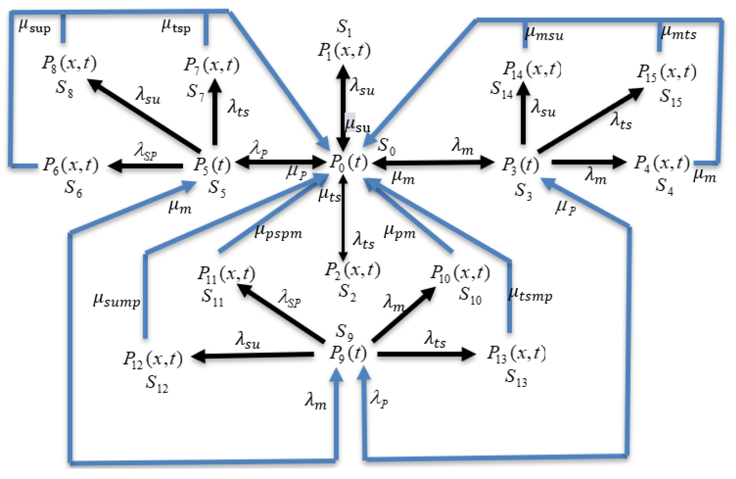
3. Mathematical Modeling Approach of the WSN and Solution

The mathematical modeling of a WSN, utilizing the concept of the continuous-time Markov process, has been performed by considering different units’ failure and repair. Once a failure or repair takes place, the system moves from one state to another state. The different state and their interconnections are shown in Figure 3, which is the transition state diagram of the WSN. Considering the defined notations and the state transition in the WSN within a given time frame, the following set of differential equations, also known as Chapman–Kolmogorov equations, is derived.

The probability that the WSN is in the state $P_0\left(t\right)$ (Figure 3) in the interval $(t,t+\Delta t)$ is given as

$$\begin{array}{c}\hfill P_0(t+\Delta t)=(1-{\lambda }_m\Delta t)(1-{\lambda }_{su}\Delta t)(1-{\lambda }_{ts}\Delta t)(1-{\lambda }_p\Delta t)P_0\left(t\right)+{\mu }_m{P}_3\left(t\right)\Delta t\\ \hfill +{\mu }_p{P}_5\left(t\right)\Delta t+\sum _{i,j}{\int }_0^{\infty }{\mu }_i{P}_j(x,t)\Delta tdx\end{array}$$

$$\begin{array}{c}\hfill P_0(t+\Delta t)=(1-{\lambda }_m\Delta t)(1-{\lambda }_{su}\Delta t)(1-{\lambda }_{ts}\Delta t)(1-{\lambda }_p\Delta t)P_0\left(t\right)+{\mu }_m{P}_3\left(t\right)\Delta t\\ \hfill +{\mu }_p{P}_5\left(t\right)\Delta t+\sum _{i,j}{\int }_0^{\infty }{\mu }_i{P}_j(x,t)\Delta tdx\end{array}$$

$$\begin{array}{c}\hfill {\displaystyle \frac{P_0(t+\Delta t)-P_0\left(t\right)}{\Delta t}}+({\lambda }_m+{\lambda }_{su}+{\lambda }_{ts}+{\lambda }_p)P_0\left(t\right)={\mu }_m{P}_3\left(t\right)\\ \hfill +{\mu }_p{P}_5\left(t\right)+\sum _{i,j}{\int }_0^{\infty }{\mu }_i{P}_j(x,t)dx\end{array}$$

$$\begin{array}{c}\hfill \underset{\Delta t\to 0}{lim}{\displaystyle \frac{P_0(t+\Delta t)-P_0\left(t\right)}{\Delta t}}+({\lambda }_m+{\lambda }_{su}+{\lambda }_{ts}+{\lambda }_p)P_0\left(t\right)={\mu }_m{P}_3\left(t\right)\\ \hfill +{\mu }_p{P}_5\left(t\right)+\sum _{i,j}{\int }_0^{\infty }{\mu }_i{P}_j(x,t)dx\end{array}$$

$$\begin{array}{cc}\hfill & \left({\displaystyle \frac{d}{dt}}+{\lambda }_m+{\lambda }_{su}+{\lambda }_{ts}+{\lambda }_p\right)P_0\left(t\right)={\mu }_m{P}_3\left(t\right)+{\mu }_p{P}_5\left(t\right)+\sum _{i,j}{\int }_0^{\infty }{\mu }_i{P}_j(x,t)dx\hfill \end{array}$$

(4)

where i= su, ts, m, psp, tsp, sup, pm, pspm, supm, tsmp, msu, mts, j = 1, 2, 4, 6, 7, 8, 10, 11, 12, 13, 14, 15.

Similarly, the Chapman–Kolmogorov equations for other states are obtained as follows.

$$\left({\displaystyle \frac{d}{dt}}+{\mu }_m+{\lambda }_m+{\lambda }_{su}+{\lambda }_{ts}+{\lambda }_p\right)P_3\left(t\right)={\lambda }_m{P}_0\left(t\right)+{\mu }_p{P}_9\left(t\right)$$

(5)

$$\left({\displaystyle \frac{d}{dt}}+{\mu }_p+{\lambda }_{sp}+{\lambda }_{ts}+{\lambda }_{su}+{\lambda }_m\right)P_5\left(t\right)={\lambda }_p{P}_0\left(t\right)+{\mu }_m{P}_9\left(t\right)$$

(6)

$$\left({\displaystyle \frac{d}{dt}}+{\mu }_m+{\mu }_p+{\lambda }_{sp}+{\lambda }_{su}+{\lambda }_{ts}+{\lambda }_m\right)P_9\left(t\right)={\lambda }_p{P}_3\left(t\right)+{\lambda }_m{P}_5\left(t\right)$$

(7)

$$\left({\displaystyle \frac{\partial }{\partial t}}+{\displaystyle \frac{\partial }{\partial x}}+{\mu }_i\right)P_j(x,t)=0$$

(8)

where i = su, ts, m, psp, tsp, sup, pm, pspm, sump, tsmp, msu, mts, j = 1, 2, 3, 4, 5, 6, 7, 8, 9, 10, 11, 12, 13, 14, 15.

$$P_i\left(t\right)=\left\{\begin{array}{cc}1,\hfill & \hfill \mathrm{if}i=0,t=0\\ 0,\hfill & \hfill \mathrm{otherwise}\end{array}\right.$$

(9)

$$P_k(0,t)={\lambda }_{su}{P}_l\left(t\right)$$

(10)

where k = 1, 8, 12, 14; l = 0, 5, 9, 3.

$$P_m(0,t)={\lambda }_{ts}{P}_n\left(t\right)$$

(11)

where m = 2, 7, 13, 15; n = 0, 5, 9, 3.

$$P_q(0,t)={\lambda }_m{P}_r\left(t\right)$$

(12)

where q = 4, 10; r = 3, 9.

$$P_u(0,t)={\lambda }_m{P}_v\left(t\right)$$

(13)

where u = 4, 10; v = 3, 9.

Taking the Laplace transformations of Equations (4)–(13) and solving the obtained equations, the authors find out the various state probabilities of the WSN, as given below (Equations (14)–(17)).

$$\overline{P_0}\left(s\right)={\displaystyle \frac{1}{\left(s+A_4-\frac{{\mu }_{su}·{\lambda }_{su}}{s+{\mu }_{su}}-\frac{{\mu }_{ts}·{\lambda }_{ts}}{s+{\mu }_{ts}}-C_4{C}_1-C_2{C}_6-C_4{C}_5-C_3\right)}}$$

(14)

$$\overline{P_3}\left(s\right)=C_5\overline{P_0}\left(s\right)$$

(15)

$$\overline{P_5}\left(s\right)=C_7\overline{P_0}\left(s\right)$$

(16)

$$\overline{P_9}\left(s\right)=C_6\overline{P_0}\left(s\right)$$

(17)

where

$$A_1={\mu }_m+{\lambda }_m+{\lambda }_{su}+{\lambda }_{ts}+{\lambda }_p$$

$$A_2={\mu }_p+{\lambda }_{sp}+{\lambda }_{ts}+{\lambda }_{su}+{\lambda }_m$$

$$A_3={\mu }_m+{\mu }_p+{\lambda }_{sp}+{\lambda }_{su}+{\lambda }_{ts}+{\lambda }_m$$

$$A_4={\lambda }_m+{\lambda }_{su}+{\lambda }_{ts}+{\lambda }_p$$

$$C_1=({\mu }_p+({\lambda }_{sp}·{\mu }_{sp})/(s+{\mu }_{sp})+({\lambda }_{ts}·{\mu }_{ts})/(s+{\mu }_{ts})+({\lambda }_{su}·{\mu }_{sup})/(s+{\mu }_{sup}))$$

$$C_2=\left({\displaystyle \frac{{\lambda }_m·{\mu }_{pm}}{s+{\mu }_{pm}}}+{\displaystyle \frac{{\lambda }_{sp}·{\mu }_{pspm}}{s+{\mu }_{pspm}}}+{\displaystyle \frac{{\lambda }_{su}·{\mu }_{sump}}{s+{\mu }_{sump}}}+{\displaystyle \frac{{\lambda }_{ts}·{\mu }_{tsmp}}{s+{\mu }_{tsmp}}}\right)$$

$$C_3=\left({\displaystyle \frac{{\lambda }_{su}·{\mu }_{su}}{s+{\mu }_{su}}}+{\displaystyle \frac{{\lambda }_{ts}·{\mu }_{ts}}{s+{\mu }_{ts}}}\right)$$

$$C_4=\left({\mu }_m+{\displaystyle \frac{{\lambda }_m·{\mu }_m}{s+{\mu }_m}}+{\displaystyle \frac{{\lambda }_{su}·{\mu }_{msu}}{s+{\mu }_{msu}}}+{\displaystyle \frac{{\lambda }_{ts}·{\mu }_{mts}}{s+{\mu }_{mts}}}\right)$$

$$C_5=\left({\displaystyle \frac{{\lambda }_m}{s+A_1}}+{\displaystyle \frac{\frac{{\mu }_p}{(s+A_1)}\left[\frac{{\lambda }_p·{\lambda }_m}{\left(s+A_1\right)}+\frac{{\lambda }_p·{\lambda }_m}{\left(s+A_2\right)}\right]}{\left(s+A_3-\frac{{\lambda }_p·{\mu }_p}{(s+A_1)}-\frac{{\mu }_m·{\lambda }_m}{\left(s+A_2\right)}\right)}}\right)$$

$$C_6=\left({\displaystyle \frac{\left[\frac{{\lambda }_p·{\lambda }_m}{\left(s+A_1\right)}+\frac{{\lambda }_p·{\lambda }_m}{\left(s+A_2\right)}\right]}{\left(s+A_3-\frac{{\lambda }_p·{\mu }_p}{(s+A_1)}-\frac{{\mu }_m·{\lambda }_m}{\left(s+A_2\right)}\right)}}\right)$$

$$C_7=\left({\displaystyle \frac{{\lambda }_p}{s+A_2}}+{\displaystyle \frac{\frac{{\mu }_m}{(s+A_2)}\left[\frac{{\lambda }_p·{\lambda }_m}{\left(s+A_1\right)}+\frac{{\lambda }_p·{\lambda }_m}{\left(s+A_2\right)}\right]}{\left(s+A_3-\frac{{\lambda }_p·{\mu }_p}{(s+A_1)}-\frac{{\mu }_m·{\lambda }_m}{\left(s+A_2\right)}\right)}}\right)$$

The probabilities that the system is in operational mode (i.e., either in a good or degraded state) and failure mode at any time t is given in Equations (18) and (19).

$${\overline{P}}_{up}\left(s\right)={\overline{P}}_0\left(s\right)+{\overline{P}}_3\left(s\right)+{\overline{P}}_5\left(s\right)+{\overline{P}}_9\left(s\right)$$

(18)

$$\begin{array}{c}\hfill {\overline{P}}_{down}\left(s\right)=\sum _{i=1,2,4,6,7,8}{\overline{P}}_i(x,s)+\sum _{j=10,11,12,13,14,15}{\overline{P}}_j(x,s)\end{array}$$

(19)

4. Calculation of Various Reliability Indices

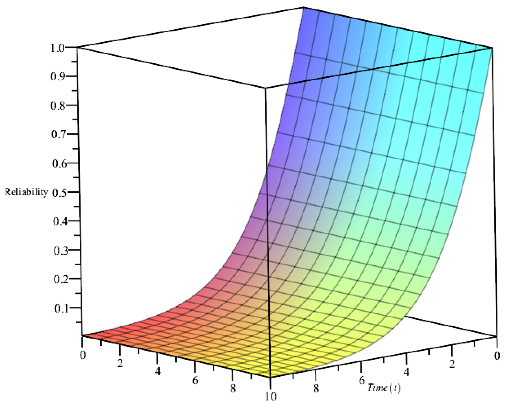
4.1. Reliability of the WSN

The reliability of the system is the probability that the system will perform adequately under given conditions and for a specified period. Mathematically, it is a probability function $R:t\to [0,1]$, which gives the probability of a system that it will work failure-free at a time t. Here, the reliability expression of the WSN is obtained, by using Equation (18), and is shown in Equation (20). Also, the time-dependent reliability expression of the WSN corresponding to a particular value of the failure rate ${\lambda }_{su}=0.22$, ${\lambda }_{ts}=0.15$, ${\lambda }_m=0.35$, ${\lambda }_p=0.03$, ${\lambda }_{sp}=0.02$ [17] is given by Equation (21).

$$\begin{array}{cc}\hfill & R\left(t\right)={\displaystyle \frac{({-e}^{-\left({\lambda }_m+{\lambda }_{su}+{\lambda }_{ts}+{\lambda }_m\right)t}{\lambda }_{sp}+e^{-\left({\lambda }_{sp}+{\lambda }_{su}+{\lambda }_{ts}+{\lambda }_m\right)t}{\lambda }_p)(t{\lambda }_m+1)}{-{\lambda }_{sp}+{\lambda }_p}}\hfill \end{array}$$

(20)

$$\begin{array}{cc}\hfill & R\left(t\right)=100(-0.02e^{-0.75t}+0.03e^{-0.74t})(0.35t+1)\hfill \end{array}$$

(21)

The graphical representation of the reliability of the WSN can be obtained by varying the t in Equation (21). It is shown in Figure 4.

For more insight about the reliability of the WSN with respect to different failures, the author investigated the component-wise reliability of the WSN.

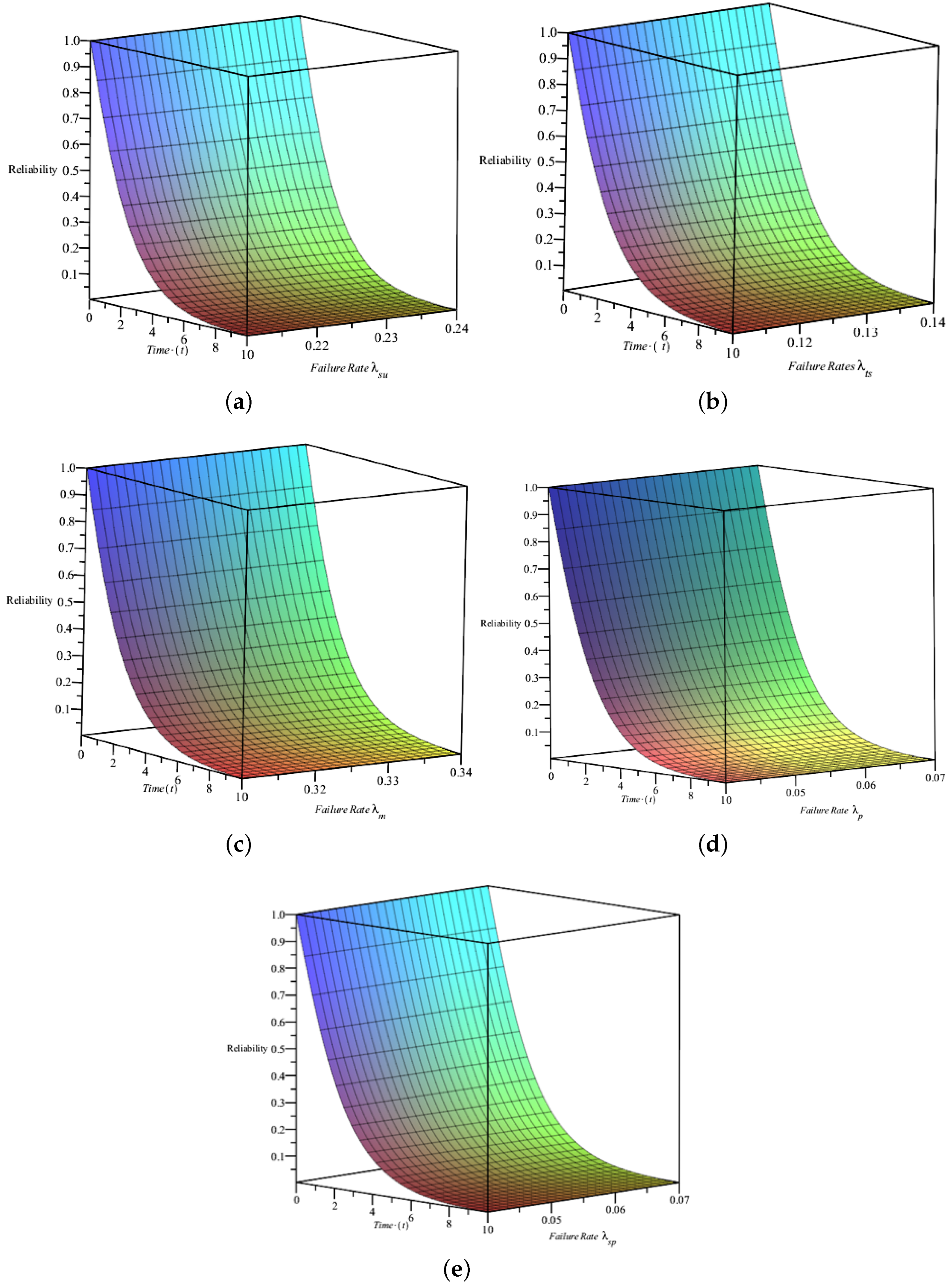
4.1.1. WSN Reliability with Fluctuation in Sensing Unit Failure

The reliability of the WSN with respect to the sensing unit is obtained by varying the failure rate of the sensing unit between 0.21, 0.22, 0.23, and 0.24 and keeping the other failure rates fixed in the reliability expression obtained in Equation (20). The obtained results are reflected in Figure 5a.

4.1.2. WSN Reliability with Fluctuation in Transceiver Failure

The reliability of the WSN with respect to the transceiver is obtained by varying the failure rate of the transceiver between 0.11, 0.12, 0.13, and 0.14 and keeping other failure rates fixed in the reliability expression obtained in Equation (20). The obtained results are reflected in Figure 5b.

4.1.3. WSN Reliability with Fluctuation in Microcontroller Failure

A microcontroller is an essential component of a wireless sensor network. To understand the reliability of the WSN with microcontroller failure, the author varied the failure rate of the microcontroller between 0.31, 0.32, 0.33, and 0.34 and kept the other failure rates fixed in the reliability expression obtained in Equation (20). The obtained results are graphically represented in Figure 5c.

4.1.4. WSN Reliability with Fluctuation in Power Unit Failure

The power supply plays a crucial role in the performance of the WSN. To optimize the operation of a WSN network, a standby power supply is one alternate option. Here, in the considered WSN, the author has considered the power supply as the main power supply and the standby power supply. The effect of the power supply/standby power supply failure on WSN reliability has been studied by varying it between 0.04, 0.05, 0.06, and 0.07 in the reliability expression obtained in Equation (20). The behavior is shown in Figure 5d and Figure 5e, respectively.

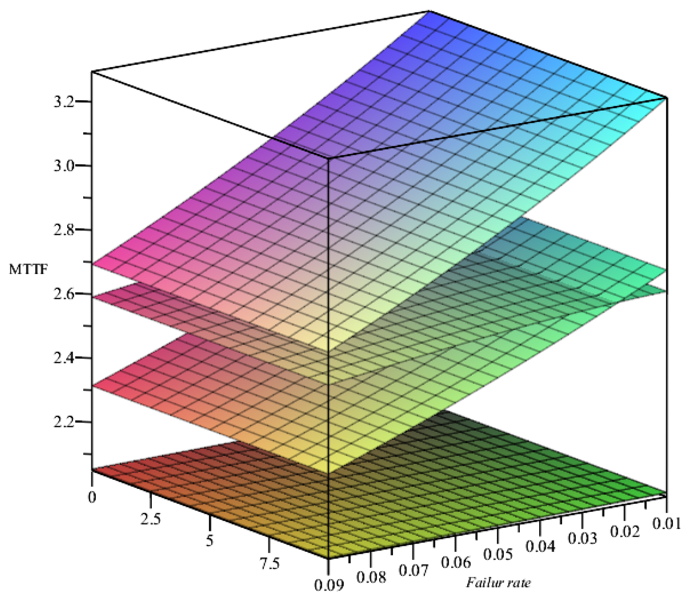
4.2. Mean Time to Failure (MTTF) Analysis

This is a measure of elapsed time between inherent systems during regular system operation. If $R\left(t\right)$ is the reliability function as obtained in Equation (20), then the mean time to failure (MTTF) for the considered system is given as Equation (22).

$$\begin{array}{cc}& \mathrm{MTTF}={\int }_0^{\infty }\mathit{t}\mathit{f}\left(\mathit{t}\right)\mathit{d}\mathit{t}={\int }_0^{\infty }\mathit{R}\left(\mathit{t}\right)\mathit{d}\mathit{t}\hfill \end{array}$$

$$\begin{array}{c}\hfill \mathrm{MTTF}={\displaystyle \frac{1}{{\lambda }_m+{\lambda }_{\mathit{su}}+{\lambda }_{\mathit{ts}}+{\lambda }_p}}+{\displaystyle \frac{{\lambda }_m}{{\left({\lambda }_m+{\lambda }_{\mathit{su}}+{\lambda }_{\mathit{ts}}+{\lambda }_p\right)}^2}}\\ \hfill +{\displaystyle \frac{{\lambda }_p}{\left({\lambda }_{\mathit{sp}}+{\lambda }_{\mathit{su}}+{\lambda }_{\mathit{ts}}+{\lambda }_m\right)\left({\lambda }_m+{\lambda }_{\mathit{su}}+{\lambda }_{\mathit{ts}}+{\lambda }_p\right)}}\\ \hfill +{\displaystyle \frac{\frac{{\lambda }_p{\lambda }_m}{{\lambda }_m+{\lambda }_{\mathit{su}}+{\lambda }_{\mathit{ts}}+{\lambda }_p}+\frac{{\lambda }_p{\lambda }_m}{{\lambda }_{\mathit{sp}}+{\lambda }_{\mathit{su}}+{\lambda }_{\mathit{ts}}+{\lambda }_m}}{\left({\lambda }_{\mathit{sp}}+{\lambda }_{\mathit{su}}+{\lambda }_{\mathit{ts}}+{\lambda }_m\right)\left({\lambda }_m+{\lambda }_{\mathit{su}}+{\lambda }_{\mathit{ts}}+{\lambda }_p\right)}}\end{array}$$

(22)

Now, substituting different values for the parameters, i.e., ${\lambda }_{su}=0.22$, ${\lambda }_{ts}=0.15$, ${\lambda }_m=0.35$, ${\lambda }_p=0.03$, and ${\lambda }_{sp}=0.02$, and varying each failure rate from 0.01 to 0.09 one by one while keeping other failure rates fixed, one can obtain a graphical representation and estimation of MTTF, as shown in

Table 3. MTTF with different unit failure rates.

Failure Rate	${\mathit{\lambda }}_{\mathit{s}\mathit{u}}$	${\mathit{\lambda }}_{\mathit{t}\mathit{s}}$	${\mathit{\lambda }}_{\mathit{m}}$	${\mathit{\lambda }}_{\mathit{p}}$	${\mathit{\lambda }}_{\mathit{s}\mathit{p}}$
0.01	3.29411	2.75676	2.69047	2.06279	2.06219
0.02	3.20597	2.69303	2.68534	2.06158	2.0604
0.03	3.12205	2.63197	2.6774	2.0604	2.05867
0.04	3.04208	2.57342	2.66707	2.05926	2.05699
0.05	2.96579	2.51725	2.6547	2.05816	2.05536
0.06	2.89295	2.46331	2.64062	2.05709	2.05378
0.07	2.82334	2.41148	2.62509	2.05605	2.05225
0.08	2.75676	2.36165	2.60833	2.05505	2.05076
0.09	2.69303	2.3137	2.59055	2.05407	2.04932

and Figure 6.

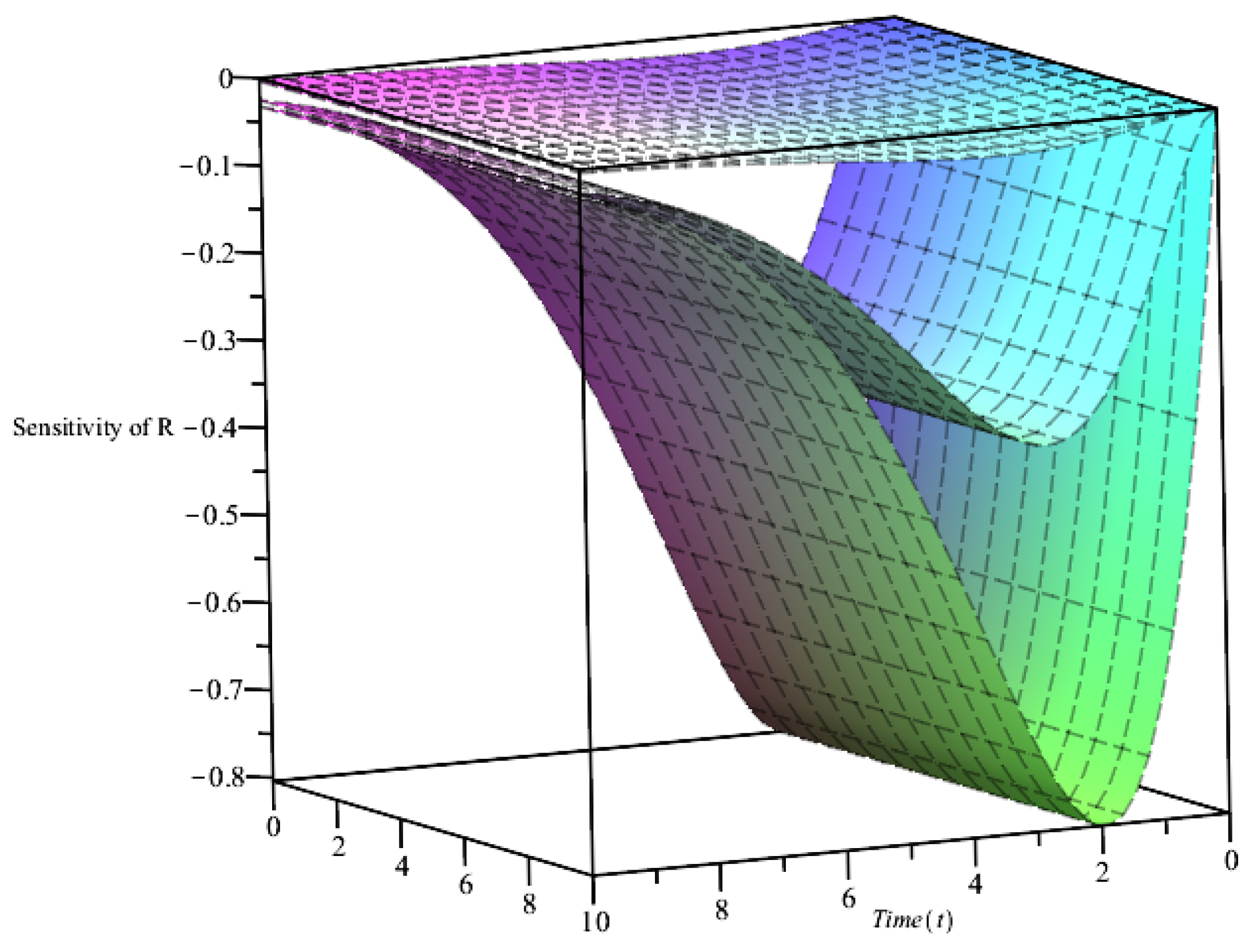
4.3. Sensitivity Analysis

Sensitivity analysis is a methodology aimed at understanding how different values of independent factors impact a particular dependent factor under some constraints. It is very effective when one wants to understand the effects of different components’ failures on the overall performance of the system. In the literature, it is used to identify the most/least critical component of a system. Here, the authors performed sensitivity analysis for WSN reliability and MTTF.

Sensitivity Analysis for Reliability of the WSN

Sensitivity analysis for reliability was performed by differentiating Equation (20) partially with respect to different failure rates and then inputting various failure rates, such as ${\lambda }_{su}=0.22$, ${\lambda }_{ts}=0.15$, ${\lambda }_m=0.35$, ${\lambda }_p=0.03$, and ${\lambda }_{sp}=0.02$, in the partial derivative expression. One can easily derive Figure 7 for the sensitivity of reliability by varying the time unit t.

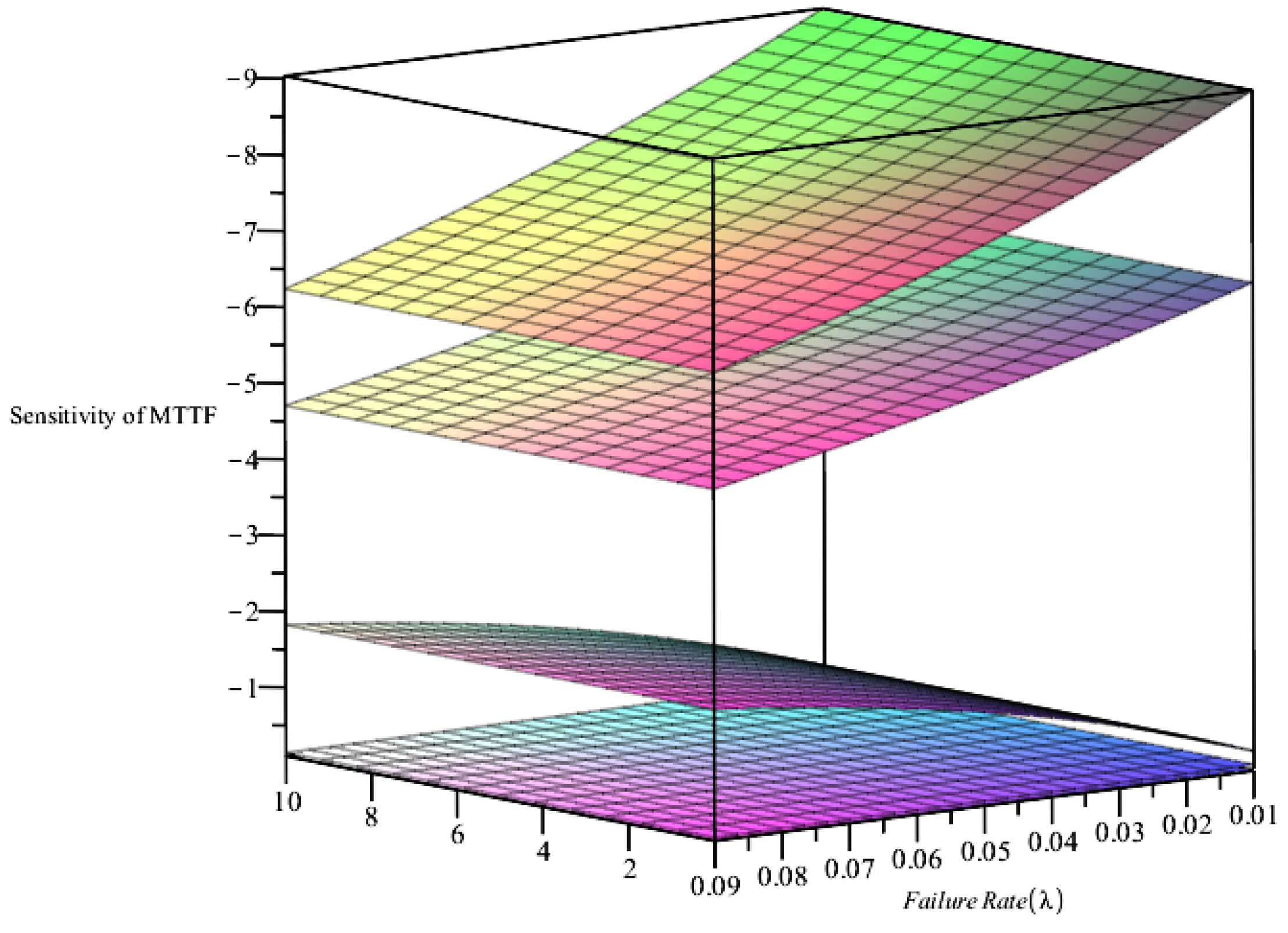
4.4. Sensitivity Analysis for MTTF of WSN

The sensitivity analysis of the WSN for MTTF is performed by partially differentiating the MTTF expression (22) with respect to different failure rates and then substituting failure rates, such as ${\lambda }_{su}=0.22$, ${\lambda }_{ts}=0.15$, ${\lambda }_m=0.35$, ${\lambda }_p=0.03$, and ${\lambda }_{sp}=0.02$ in the partial derivatives. Figure 8 demonstrates how different components affect the MTTF of the WSN.

5. Results Discussion

In the present paper, the authors carried out a performance analysis of the wireless sensor network by using the concept of continuous-time Markov process and Chapman–Kolmogorov equations. Figure 4 represents the behavior of the WSN’s reliability with the time unit. From this figure, it has been observed that the reliability initially decreases rapidly as time passes, and later on becomes constant. At $t=1$, $R=0.653414$ and at $t=10$, $R=0.003274$. The reliability of wireless sensor network systems is majorly affected by the failure rates of their different components. The behaviors of WSN reliability with respect to different components, e.g., the sensing unit, transceiver, microcontroller, power unit, and stand-by power unit, are shown in Figure 5. The obtained reliability values at time 10 units show degradation of the system with failure rates of the component. Figure 6 revealed the results for the MTTF of the WSN. It is observed that the MTTF is highest for the failure rate of the sensing unit. The MTTF is almost constant despite variations in the failure rates of the power and stand-by power unit. Sensitivity analysis for the WSN in the context of reliability and MTTF has been performed in this study. Figure 7 represents the sensitivity of reliability. It shows that the WSN reliability is highly affected by the failure of the sensing unit and transceiver. From the graph, it is observed that the power unit and stand-by power unit are the least sensitive components. The sensitivity analysis of MTTF is reflected in Figure 8. It shown that the WSN’s MTTF is highly affected by the failure rates of transceivers and microcontroller.

6. Conclusions

A stochastic model has been developed for reliability and sensitivity analysis of a wireless sensor network (WSN), using a continuous-time Markov approach, and the explicit expressions for state probabilities have been derived. Based on performed calculations and results discussion in Section 5, it is concluded that the reliability of the wireless sensor network shows a rapid decline as time passes. To improve the reliability of the WSN, more attention to the maintenance strategy should be aligned for the sensing unit and microcontroller unit, or some redundancy could be added at system level. Also, to improve the WSN’s MTTF, transceiver and microcontroller failures must be optimized. For an efficient system, proper maintenance at the right time is crucial. The presented research, which emphasizes various performance measures of the WSN, will be helpful for system designers and beneficial to the wireless sensor network industry.

References

1. Kandris, D.; Nakas, C.; Vomvas, D.; Koulouras, G. Applications of wireless sensor networks: An up-to-date survey. J. Appl. Syst. Innov. 2020, 3, 14. [Google Scholar] [CrossRef]
2. Baduge, S.K.; Thilakarathna, S.; Perera, J.S.; Arashpour, M.; Sharafi, P.; Teodosio, B.; Shringi, A.; Mendis, P. Artificial intelligence and smart vision for building and construction 4.0: Machine and deep learning methods and applications. Autom. Constr. 2022, 141, 104440. [Google Scholar] [CrossRef]
3. Adu-Manu, K.S.; Abdulai, J.D.; Engmann, F.; Akazue, M.; Appati, J.K.; Baiden, G.E.; Sarfo-Kantanka, G. WSN architectures for environmental monitoring applications. J. Sens. 2022, 1, 7823481. [Google Scholar] [CrossRef]
4. Chowdhury, M.Z.; Shahjalal, M.; Ahmed, S.; Jang, Y.M. 6G wireless communication systems: Applications, requirements, technologies, challenges, and research directions. IEEE Open J. Commun. Soc. 2020, 1, 957–975. [Google Scholar] [CrossRef]
5. Khalifeh, A.; Mazunga, F.; Nechibvute, A.; Nyambo, B.M. Microcontroller unit-based wireless sensor network nodes: A review. Sensors 2022, 22, 8937. [Google Scholar] [CrossRef] [PubMed]
6. Lanzolla, A.; Spadavecchia, M. Wireless sensor networks for environmental monitoring. Sensors 2022, 21, 1172. [Google Scholar] [CrossRef]
7. Patel, N.; Rai, R.N.; Patil, H.; Shrivastava, P. Reliability Analysis of Cutting Tools for Industrial Applications: An Integrated AHP-RSM-PHM Approach. Int. J. Math. Eng. Manag. Sci. 2024, 9, 756–778. [Google Scholar] [CrossRef]
8. de Vasconcelos, V.; Soares, W.A.; da Costa, A.C.L.; Raso, A.L. Use of Reliability Block Diagram and Fault Tree Techniques in Reliability Analysis of Emergency Diesel Generators of Nuclear Power Plants. Int. J. Math. Eng. Manag. Sci. 2019, 4, 814–823. [Google Scholar] [CrossRef]
9. Chachra, A.; Ram, M.; Kumar, A. Fuzzy reliability framework under hesitant and dual hesitant fuzzy sets to air conditioning system. Opsearch 2024, 61, 603–627. [Google Scholar] [CrossRef]
10. Arjannikov, T.; Diemert, S.; Ganti, S.; Lampman, C.; Wiebe, E.C. Using markov chains to model sensor network reliability. In Proceedings of the 12th International Conference on Availability, Reliability and Security, New York, NY, USA, 29 August–1 September 2017; pp. 1–10. [Google Scholar]
11. Oreku, G.S. Reliability in WSN for security: Mathematical approach. In Proceedings of the 2013 International Conference on Computer Applications Technology (ICCAT), Sousse, Tunisia, 20–22 January 2013; pp. 1–6. [Google Scholar]
12. Mishra, P.; Dash, R.K. A novel method for evaluation of reliability of WSN under different failure models. In Proceedings of the 2020 IEEE International Symposium on Sustainable Energy, Signal Processing and Cyber Security (iSSSC), Odisa, India, 16 December 2020; pp. 1–6. [Google Scholar]
13. Shrestha, A.; Xing, L.; Liu, H. Modeling and evaluating the reliability of wireless sensor networks. In Proceedings of the 2007 Annual Reliability and Maintainability Symposium, Orlando, FL, USA, 22–25 January 2007; pp. 186–191. [Google Scholar]
14. Kabashkin, I.; Kundler, J. Reliability of sensor nodes in wireless sensor networks of cyber physical systems. Procedia Comput. Sci. 2017, 104, 380–384. [Google Scholar] [CrossRef]
15. Silva, I.; Guedes, L.A.; Portugal, P.; Vasques, F. Reliability and availability evaluation of wireless sensor networks for industrial applications. Sensors 2012, 12, 806–838. [Google Scholar] [CrossRef] [PubMed]
16. Dâmaso, A.; Rosa, N.; Maciel, P. Reliability of wireless sensor networks. Sensors 2014, 14, 15760–15785. [Google Scholar] [CrossRef] [PubMed]
17. Catelani, M.; Ciani, L.; Bartolini, A.; Del Rio, C.; Guidi, G.; Patrizi, G. Reliability analysis of wireless sensor network for smart farming applications. Sensors 2021, 21, 7683. [Google Scholar] [CrossRef] [PubMed]
18. Jung, S.; Choi, J.P. End-to-end reliability of satellite communication network systems. IEEE Syst. J. 2020, 15, 791–801. [Google Scholar] [CrossRef]
19. Joshi, T.; Goyal, N.; Ram, M. An approach to analyze reliability indices in peer-to-peer communication systems. Cybern. Syst. 2022, 53, 716–733. [Google Scholar] [CrossRef]
20. Ram, M.; Tyagi, V.; Rawat, N. Reliability modelling and sensitivity analysis of IOT based flood alerting system. J. Qual. Maint. Eng. 2021, 27, 292–307. [Google Scholar]
21. Singh, V.V.; Poonia, P.K.; Rawal, D.K. Reliability analysis of repairable network system of three computer labs connected with a server under 2-out-of-3 G configuration. Life Cycle Reliab. Saf. Eng. 2021, 10, 19–29. [Google Scholar] [CrossRef]
22. Kumar, A.; Kumar, P. Application of markov process/mathematical modelling in analysing communication system reliability. Int. J. Qual. Reliab. Manag. 2020, 37, 354–371. [Google Scholar] [CrossRef]
23. Bisht, S.; Kumar, A.; Goyal, N.; Ram, M.; Klochkov, Y. Analysis of network reliability characteristics and importance of components in a communication network. Mathematics 2021, 9, 1347. [Google Scholar] [CrossRef]
24. Shunqi, Y.; Ying, Z.; Xiang, L.; Yanfeng, L.; Hongzhong, H. Reliability analysis for wireless communication networks via dynamic Bayesian network. J. Syst. Eng. Electron. 2023, 34, 1368–1374. [Google Scholar] [CrossRef]
25. Poonia, P.K. Performance assessment and sensitivity analysis of a computer lab network through copula repair with catastrophic failure. J. Reliab. Stat. Stud. 2022, 15, 105–128. [Google Scholar] [CrossRef]
26. Xing, L. Reliability in Internet of Things: Current status and future perspectives. IEEE Internet Things J. 2020, 7, 6704–6721. [Google Scholar] [CrossRef]
27. Kumar, P.; Kumar, A. Quantifying reliability indices of garbage data collection iot-based sensor systems using markov birth-death process. Int. J. Math. Eng. Manag. Sci. 2023, 8, 1255–1274. [Google Scholar] [CrossRef]
28. Xing, L.; Zhao, G.; Xiang, Y.; Liu, Q. A behavior-driven reliability modeling method for complex smart systems. Qual. Reliab. Eng. Int. 2021, 37, 2065–2084. [Google Scholar] [CrossRef]
29. Choudhary, S.; Ram, M.; Goyal, N.; Saini, S. Reliability Analysis of Mobile Communication System using Markov Process. In Proceedings of the 2022 2nd International Conference on Innovative Sustainable Computational Technologies (CISCT), Dehradun, India, 23–24 December 2022; pp. 1–5. [Google Scholar]
30. Wang, C.; Xing, L.; Vokkarane, V.M.; Sun, Y. Infrastructure communication sensitivity analysis of wireless sensor networks. Qual. Reliab. Eng. Int. 2016, 32, 581–594. [Google Scholar] [CrossRef]
31. Chakraborty, S.; Goyal, N.K.; Mahapatra, S.; Soh, S. Monte-Carlo Markov chain approach for coverage-area reliability of mobile wireless sensor networks with multistate nodes. Reliab. Eng. Syst. Saf. 2020, 193, 106662. [Google Scholar] [CrossRef]
32. Gupta, N.; Saini, M.; Kumar, A. Operational availability analysis of generators in steam turbine power plants. SN Appl. Sci. 2020, 2, 779. [Google Scholar] [CrossRef]
33. Kijima, M. Markov Processes for Stochastic Modeling; Springer: New York, NY, USA, 2013; pp. 1–23. [Google Scholar]
34. Lbe, O. Fundamentals of Applied Probability and Random Processes, 2nd ed.; Academic Press: Cambridge, MA, USA, 2014; pp. 358–376. [Google Scholar]
Figure 1. Applications of wireless sensor networks.
Mathematics 12 03057 g001
Figure 2. Flow diagram of a WSN.
Mathematics 12 03057 g002
Figure 3. State transition diagram of the WSN.
Mathematics 12 03057 g003
Figure 4. Behavior of reliability of the WSN.
Mathematics 12 03057 g004
Figure 5. (a) Reliability vs. λ s u . (b) Reliability vs. λ t s . (c) Reliability vs. λ m . (d) Reliability vs. λ p . (e) Reliability vs. λ s p .
Mathematics 12 03057 g005
Figure 6. Behavior of the WSN’s MTTF with different unit failure rates.
Mathematics 12 03057 g006
Figure 7. Sensitivity for reliability of the WSN.
Mathematics 12 03057 g007
Figure 8. Sensitivity for the WSN’s MTTF.
Mathematics 12 03057 g008