Dynamic Analysis and Approximate Solution of Transient Stability Targeting Fault Process in Power Systems

Abstract

Modern power systems are high-dimensional, strongly coupled nonlinear systems with complex and diverse dynamic characteristics. The polynomial model of the power system is a key focus in stability research. Therefore, this paper presents a study on the approximate transient stability solution targeting the fault process in power systems. Firstly, based on the inherent sinusoidal coupling characteristics of the power system swing equations, a generalized polynomial matrix description in perturbation form is presented using the Taylor expansion formula. Secondly, considering the staged characteristics of the stability process in power systems, the approximate solutions of the polynomial model during and after the fault are provided using coordinate transformation and regular perturbation techniques. Then, the structural characteristics of the approximate solutions are analyzed, revealing the mathematical basis of the stable motion patterns of the power grid, and a monotonicity rule of the system’s power angle oscillation amplitude is discovered. Finally, the effectiveness of the proposed methods and analyses is further validated by numerical examples of the IEEE 3-machine 9-bus system and IEEE 10-machine 39-bus system.

1. Introduction

Modern power systems, under the new configuration of hybrid AC/DC grids with large-scale wind and solar power integration, exhibit complex and diverse dynamic characteristics. As the coupling between sending and receiving ends intensifies, the uncertainty of large disturbances increases, reducing stability margins. High proportions of renewable energy and power electronic devices are reshaping grid stability characteristics by mimicking the stability mechanisms of synchronous machines over shorter time scales, thus highlighting stability issues in power systems [1]. Among these issues, the transient stability hidden behind synchronous machines warrants particular attention. The rotor swing equation, underlying transient stability phenomena, is a key factor in understanding the dynamic characteristics of synchronous grids. It profoundly influences multiple transient stability issues, such as power angle stability and frequency stability, controlling the dynamic response of power systems under various disturbances. Therefore, unveiling its characteristics is crucial for a deeper understanding of the operational principles of synchronous grids and for ensuring the safe and stable operation of power systems [2,3].

The development of perturbation theory can be traced back to the 18th and 19th centuries, when significant contributions were made by Laplace, Lagrange, Poincaré, and others. While studying complex celestial orbits, they developed a set of asymptotic expansion methods based on small parameters. The analytical study of swing equations originated from one of these branches of asymptotic expansion methods. Its core idea involves expanding curves as a sum of finite terms of small parameters, thereby obtaining analytical solutions to initial-value problems of ordinary differential equations. This idea gradually matured and formed an independent modern mathematical theory system [4]. Starting from 1995, scholars such as Saha S and Vittal V realized the inherent nonlinearity of swing equations, making accurate solutions difficult to obtain. They began attempting methods like the normal form to find stable manifolds of unstable equilibrium points of nonlinear power system swing equations [5,6,7,8]. This gained widespread attention from researchers studying power system stability boundaries, further developing in the visualization, approximate estimation, and expression analysis of stability boundaries [9,10,11]. The proposal of the quadratic approximation formula for nonlinear dynamical system stability boundaries enabled it to directly serve as an analytical method for power system transient stability swing equations [12]. This method, integrating the fault-clearing time and stability domain calculations through asymptotic methods, further enhanced the practical utility of analytical transient stability theory in power engineering applications [13,14].

In recent years, there have been further advancements in analytical methods for power system transient stability. Scholars such as Rui M and Meng Z, inspired by the pendulum system, have employed computational fitting to elucidate stable forms within the parameter space based on the analytical form of swing equation bifurcation curves. They conducted research on power system synchronous stability and analyzed theories involving multiple time scales. However, this method focuses more on single-machine systems; thus, its practical utility is limited [15]. Yang L and others utilized a novel non-iterative method of differential transformation to convert nonlinear terms into a series of commonly used functions, resulting in the rapid and reliable enhancement of the analytical nature of grid equations, thereby alleviating computational burdens in numerical simulations [16]. Gurunath G and others employed a multilevel homotopy method to demonstrate the influence of the time step on the solution accuracy and stability. They developed a semi-analytical form of solution and applied it to the time-domain simulation of power systems, effectively improving simulation efficiency [17].

Due to the prevalent utilization of semi-analytical methods in the above-mentioned approaches, primarily aimed at enhancing the analytical nature of swing equations to facilitate subsequent numerical simulations, the revelation of structural characteristics of power system transient stability swing equations is limited. Concurrently, the asymptotic expansion method based on the multi-timescale approach has found extensive applications in the industrial domain [18]. Considering that the solutions of lower-order equations constitute the inhomogeneous terms of higher-order equations, triggering secular terms if the oscillation frequency of the inhomogeneous terms equals the frequency of the differential operator of the higher-order equation, further advancements have been made in a series of studies based on single-degree-of-freedom systems, aiming to overcome the secular term issue faced by direct expansion methods. Examples include the multi-timescale perturbation solutions of Duffing’s equation and the analytical solutions of Mathieu’s equation based on the multi-timescale method, followed by the corresponding stability analysis [19,20,21]. This subsequently inspired research methods for both low- and high-degree-of-freedom systems, providing theoretical guidance for transient stability analysis considering the power system fault process. Examples include utilizing the multi-timescale method for the approximate analytical estimation of low-degree-of-freedom differential algebraic systems and deriving approximate perturbation solutions for weakly coupled three-degree-of-freedom linear systems [22,23].

Based on an understanding of the power system fault process, this paper, inspired by the multi-timescale method, systematically develops a highly analytical method and theory for the transient stability analysis of power grids by elucidating the research trajectory of analytical methods for swing equations and utilizing canonical perturbation methods. To sum up, the original contributions of this paper are threefold:

(1)

Polynomial Model. Based on observing the sinusoidal coupling characteristics of power grid swing equations, we employ Taylor expansion formulas to expand them into a series of homogeneous polynomials. This results in a generalized matrix description of power system swing equations in perturbation form, thus forming a polynomial mathematical model for power system transient stability.

(2)

Approximate Solution Method. During grid faults, we simplify the swing equations into a forced oscillation model and, considering the influence of faults, provide approximate solutions to power system swing equations during fault periods. After fault clearance, by introducing dual-timescale variables, we transform the nonlinear swing equations into a series of linear partial differential equations, obtaining analytical perturbation solutions to post-fault grid equations.

(3)

Application and Analysis. Theoretical analysis of approximate solutions demonstrates the rigorous mathematical foundation inherent in power system transient stability. Each solution component embodies distinct motion patterns. Furthermore, based on the structural composition of approximate solutions, we elucidate the morphological characteristics of grid stability motion. Through application to various scenarios, we explore the monotonicity patterns of power system rotor angle swing amplitudes with the fault-clearing time following major disturbances like three-phase short circuits. Finally, through simulations, we further confirm the effectiveness of theoretical analysis.

The rest of this paper is organized as follows. In Section 2, a polynomial model for power system transient stability is established, along with an introduction to the polynomial description and approximate solutions derived from the second-order Kuramoto network during the fault process. Section 3 presents the structural properties of block decoupling solutions for power system transient stability after fault clearance and provides a detailed introduction to the analytical methods for power system transient stability equations post-fault clearance. Section 4 demonstrates the application and effectiveness of power systems’ approximate transient stability solutions through multiple power system test cases. Finally, Section 5 concludes the paper.

2. The Polynomial Mathematical Description of Power Systems

In this section, the polynomial model for the transient stability of power systems is derived. This model is based on the rotor swing equations of multiple synchronous machines and is expressed in matrix form, making it applicable to Kuramoto models with an arbitrary number of oscillators. Subsequently, utilizing a coordinate transformation of rotor angles and the unique response characteristics of the system, the polynomial model is decoupled into two subsystems. Based on the characteristics of rotor angle swing amplitudes during the fault process, equations and approximate solutions for the system during faults are provided under forced oscillation conditions.

2.1. The Polynomial Model of Power Systems Based on Taylor Expansion

In synchronous power grids, when generators adopt the transient reactance constant-voltage model and loads adopt the constant-impedance model, the dynamic process of the power system after experiencing significant disturbances such as generator tripping, line-to-ground faults, and three-phase short circuits can be described by the second-order Kuramoto network model of swing equations [24], as shown in Equation (1):

$$\{\begin{array}{l}{\displaystyle \frac{2H_i}{{\omega }_R}}{\ddot{\delta }}_i+{\displaystyle \frac{D_i}{{\omega }_R}}{\dot{\delta }}_i=P_{Mi}-{\displaystyle \sum _{j=1}^{n+1}{a}_{ij}\sin \left({\delta }_{ij}-{\gamma }_{ij}\right)}\\ {\delta }_i(t_c)={\delta }_{i,0};\hspace{0.17em}\hspace{0.17em}{\dot{\delta }}_i(t_c)={\omega }_{i,0};\hspace{0.17em}\hspace{0.17em}i=1,2,\dots ,N\end{array}$$

(1)

where $H_i$ represents the moment of inertia, $D_i$ represents the damping coefficient, ${\delta }_{ij}={\delta }_i-{\delta }_j$ represents the phase angle difference, $n+1$ denotes the number of synchronous machines, ${\omega }_R$ is the reference frequency of the power grid, $P_{Mi}$ represents the mechanical power of the machine $i$, $\left({\delta }_{i,0},{\omega }_{i,0}\right)$ denotes the initial values of state variables, $a_{ij}=\left|E_i^{\prime }{Y}_{ij}{E}_j^{\prime }\right|$ represents the maximum transmission power between lines $ij$, ${\gamma }_{ij}={\varphi }_{ij}-\pi /2$, and $Y_{ij}=\left|Y_{ij}\right|\exp \left(j{\varphi }_{ij}\right)$. A schematic diagram described by Equation (1) is illustrated in Figure 1 when the number of synchronous machines $n+1=3$.

For analytical convenience, considering the weak damping characteristics of power systems, damping coefficients are neglected, and the sine function is expanded to the third order. The swing equation model can be rewritten as Equation (2):

$${\displaystyle \frac{2H_i}{{\omega }_R}}{\ddot{\delta }}_i=P_{Mi}-{\displaystyle \sum _{j=1}^{n+1}{a}_{ij}\left[{\delta }_{ij}-{\gamma }_{ij}-ϵ{\left({\delta }_{ij}-{\gamma }_{ij}\right)}^3\right]}\hspace{0.17em}\hspace{0.17em}$$

(2)

where $ϵ=1/6$, and a coordinate transformation, denoted by $y=\delta -\overline{\delta }$, is introduced, where $\overline{\delta }$ represents a specific constant vector. Consequently, the right-hand side of Equation (2) can be expressed as Equation (3):

$$\begin{array}{l}r.h.s.=P_{Mi}-{\displaystyle \sum _{j=1}^{n+1}{a}_{ij}\left[{\delta }_{ij}-{\gamma }_{ij}-ϵ{({\delta }_{ij}-{\gamma }_{ij})}^3\right]}\\ \hspace{0.17em}\hspace{0.17em}\hspace{0.17em}\hspace{0.17em}=P_{Mi}-{\displaystyle \sum _{j=1}^{n+1}{a}_{ij}\left[y_{ij}+\underset{{\eta }_{ij}}{\underbrace{{\overline{\delta }}_{ij}-{\gamma }_{ij}}}-ϵ{(y_{ij}+\underset{{\eta }_{ij}}{\underbrace{{\overline{\delta }}_{ij}-{\gamma }_{ij}}})}^3\right]}\\ \hspace{0.17em}\hspace{0.17em}\hspace{0.17em}\hspace{0.17em}=\left[\underset{P_{Meqi}}{\underbrace{P_{Mi}-{\displaystyle \sum _{j=1}^{n+1}{a}_{ij}({\eta }_{ij}-ϵ{\eta }_{ij}^3)}}}\right]-{\displaystyle \sum _{j=1}^{n+1}\left(a_{ij}-\underset{b_{ij}}{\underbrace{3ϵa_{ij}{\eta }_{ij}^2}}\right)y_{ij}}\\ \hspace{0.17em}\hspace{0.17em}\hspace{0.17em}\hspace{0.17em}\hspace{0.17em}\hspace{0.17em}\hspace{0.17em}\hspace{0.17em}\hspace{0.17em}\hspace{0.17em}\hspace{0.17em}\hspace{0.17em}\hspace{0.17em}\hspace{0.17em}\hspace{0.17em}\hspace{0.17em}\hspace{0.17em}\hspace{0.17em}\hspace{0.17em}\hspace{0.17em}\hspace{0.17em}\hspace{0.17em}\hspace{0.17em}\hspace{0.17em}\hspace{0.17em}\hspace{0.17em}\hspace{0.17em}\hspace{0.17em}\hspace{0.17em}\hspace{0.17em}\hspace{0.17em}\hspace{0.17em}\hspace{0.17em}+ϵ{\displaystyle \sum _{j=1}^{n+1}\underset{c_{ij}}{\underbrace{3a_{ij}{\eta }_{ij}}}{y}_{ij}^2}\hspace{0.17em}+ϵ{\displaystyle \sum _{j=1}^{n+1}{a}_{ij}{y}_{ij}^3}\\ \hspace{0.17em}\hspace{0.17em}\hspace{0.17em}\hspace{0.17em}=P_{Meqi}-{\displaystyle \sum _{j=1}^{n+1}\left(a_{ij}-b_{ij}\right)y_{ij}}\hspace{0.17em}+ϵ{\displaystyle \sum _{j=1}^{n+1}{c}_{ij}{y}_{ij}^2}\hspace{0.17em}+ϵ{\displaystyle \sum _{j=1}^{n+1}{a}_{ij}{y}_{ij}^3}\end{array}$$

(3)

Based on Equation (3), the swing equations for the entire system can be written in matrix form, as shown in Equation (4):

$$\begin{array}{l}M{y}^{″}=P_{Meq}-{\mathit{C}}_{1}y+ϵ{\mathit{C}}_{2}diag(Py)Py\\ \hspace{1em}\hspace{1em}\hspace{1em}\hspace{1em}\hspace{1em}\hspace{1em}+ϵ{\mathit{C}}_3{[diag(Py)]}^{2}Py\end{array}$$

(4)

where $y\in {ℝ}^{n+1}$, $M=diag(2H_1/{\omega }_R,···,2H_{n+1}/{\omega }_R)$ represents a constant diagonal matrix, $P_{Meq}={[P_{Meq,1},\dots ,P_{Meq,n+1}]}^T$ represents the equivalent mechanical power vector, and ${\mathit{C}}_2,{\mathit{C}}_3\in {ℝ}^{(n+1)\times \left[(n+1)n/2\right]}$ corresponds to the constant coefficient matrix. Also, ${\mathit{C}}_1\in {ℝ}^{(n+1)\times (n+1)}$ is defined in the following form:

$${\mathit{C}}_1=\{\begin{array}{l}{\displaystyle \sum _{j=1,j\ne i}^{n+1}{a}_{ij}-b_{ij}}\hspace{0.17em}\hspace{0.17em}\hspace{0.17em}i=j\\ \hspace{0.17em}\hspace{0.17em}\hspace{0.17em}\hspace{0.17em}\hspace{0.17em}-a_{ij}+b_{ij}\hspace{0.17em}\hspace{0.17em}\hspace{0.17em}i\ne j\end{array}$$

(5)

Furthermore, the matrix $P\in {ℝ}^{\left[(n+1)n/2\right]\times (n+1)}$ satisfies the following equation:

$$Py={\left[y_{12},···,y_{1,n+1},y_{23},···,y_{2,n+1},···,y_{n,n+1}\right]}^T$$

(6)

where $y_{ij}=y_i-y_j,1\le i<j\le n+1$ denotes the phase angle difference. It can be inferred from the aforementioned definitions that ${\mathit{C}}_1,P\in ℒ$ holds true, where $ℒ$ represents a class of matrices with zero row sums, possessing the following mathematical property:

$${\mathit{C}}_1·\mathbf{1}=P·\mathbf{1}=\mathbf{0}$$

(7)

where $\mathbf{1}$ represents a vector of appropriate dimensions consisting entirely of ones. Further simplification of Equation (7) yields Equation (8):

$$\begin{array}{l}{y}^{″}=M^{-1}{P}_{Meq}-\mathit{D}y+ϵM^{-1}{\mathit{C}}_{2}diag(Py)Py\\ \hspace{1em}\hspace{1em}\hspace{1em}\hspace{1em}\hspace{1em}\hspace{1em}+ϵM^{-1}{\mathit{C}}_3{[diag(Py)]}^{2}Py\end{array}$$

(8)

where $\mathit{D}=M^{-1}{\mathit{C}}_1$ and $\mathit{D}\in ℒ$.

2.2. Polynomial Description and Approximate Solution of Power Systems during Fault Process

Studying the stability of power systems under significant disturbances typically involves dividing the transient process into three stages:

The pre-fault system,

$$\{\begin{array}{l}\dot{\mathit{x}}=f_0(x,y,\mathit{u})\\ \mathbf{0}=g_0(x,y,\mathit{u})\end{array},\hspace{0.17em}\hspace{0.17em}\hspace{0.17em}\hspace{0.17em}\hspace{0.17em}-\infty \le t\le t_F$$

(9)

the during-fault system,

$$\{\begin{array}{l}\dot{x}=f_F(x,y,\mathit{u})\\ \mathbf{0}=g_F(x,y,\mathit{u})\end{array},\hspace{0.17em}\hspace{0.17em}\hspace{0.17em}\hspace{0.17em}\hspace{0.17em}\hspace{0.17em}{t}_F\le t<t_P$$

(10)

and the post-fault system,

$$\{\begin{array}{l}\dot{x}=f_{PF}(x,y,\mathit{u})\\ \mathbf{0}=g_{PF}(x,y,\mathit{u})\end{array},\hspace{0.17em}\hspace{0.17em}\hspace{0.17em}\hspace{0.17em}\hspace{0.17em}\hspace{0.17em}\hspace{0.17em}{t}_P\le t<\infty$$

(11)

where $x$ represents the state variables describing dynamic processes such as the generator, excitation system, and governor control; $y$ represents algebraic variables describing the voltage magnitude and phase angle at network nodes; $\mathit{u}$ represents control variables; $t_F$ denotes the initial time of fault occurrence; $t_P$ denotes the time of fault clearance; $f_0$ and $g_0$ describe the dynamic characteristics and network properties of the power system before the fault occurs; $f_F$ and $g_F$ represent the new equation structure dominating the system dynamics during the fault period due to external fault occurrence; and $f_{PF}$ and $g_{PF}$ represent the differential algebraic systems sustaining the dynamic process after fault clearance.

During the fault period, which is typically short, the generator rotor angle swing is limited. Meanwhile, let $\overline{\delta }$ denote the stable equilibrium point of the pre-fault system (9). Then, the dynamic system described by Equation (8) moves near the origin, with quadratic and cubic nonlinear effects being minimal and negligible. The swing equation can be approximated as the forced oscillation form (12):

$$y^{″}=-\mathit{D}y+M^{-1}{P}_{Meq}$$

(12)

subject to the initial condition $y(0)=\dot{y}(0)=\mathbf{0}$.

Introducing transformation $y=\mathit{U}\theta$ and performing eigenvalue decomposition on the matrix of the faulted system during the fault period, we obtain $\mathit{D}=\mathit{U}{\Lambda }_F^2{\mathit{U}}^{-1}$, where the diagonal matrix is ${\Lambda }_F^2=diag\left(0,0,\dots ,{\lambda }_{r+1}^2,\dots ,,{\lambda }_{n+1}^2\right)$. Then, the swing equation in the coordinate system $\theta$ can be expressed as Equation (13):

$${\theta }^{″}=-{\Lambda }_F^2\theta +J$$

(13)

where $J={[2J_1^T,J_2^T]}^T={\mathit{U}}^{-1}{M}^{-1}{P}_{Meq}$. Equation (13) can be further written in component form, as shown in Equation (14):

$$\{\begin{array}{l}{\theta }_1^{″}=2J_1\\ {\theta }_2^{″}=-{\lambda }_2^2{\theta }_2+J_2\end{array}$$

(14)

From Equation (14), we can observe that the solution to the system in Equation (12) during the fault period is given by

$$y=\mathit{U}\theta =\mathit{U}\left[\begin{array}{l}\hspace{0.17em}\hspace{0.17em}\hspace{0.17em}\hspace{0.17em}\hspace{0.17em}\hspace{0.17em}\hspace{0.17em}\hspace{0.17em}\hspace{0.17em}{J}_1{t}^2+{\mathit{C}}_{1}t+{\mathit{C}}_2\\ {({\lambda }_2^2)}^{-1}{J}_2+I(e^{\mathrm{i}{\lambda }_{2}t}{\mathit{C}}_3+e^{-\mathrm{i}{\lambda }_{2}t}{\mathit{C}}_4)\end{array}\right]$$

(15)

where ${\mathit{C}}_1,{\mathit{C}}_2\in {ℝ}^{r\times 1}$ and ${\mathit{C}}_3,{\mathit{C}}_4\in {ℝ}^{\left(n+1-r\right)\times 1}$ represent constant vectors determined by the initial conditions, and $I\in {ℝ}^{\left(n+1-r\right)\times \left(n+1-r\right)}$ represents the identity matrix.

Considering the initial conditions of Equation (12) to be $\mathbf{0}$, ${\mathit{C}}_1={\mathit{C}}_2=\mathbf{0}$ holds true, and the expression for ${\mathit{C}}_3,{\mathit{C}}_4$ is given by Equation (16) as follows:

$${\mathit{C}}_3={\mathit{C}}_4={\displaystyle \frac{-{({\lambda }_2^2)}^{-1}{J}_2}{2}}$$

(16)

Combining Equations (15) and (16) and defining $\mathit{U}=[{\mathit{U}}_1,{\mathit{U}}_2]$, the solution to the system in Equation (12) during the fault period can be rewritten as follows:

$$\begin{array}{l}y={\mathit{U}}_1{J}_1{t}^2+{\mathit{U}}_2{\left({\lambda }_2^2\right)}^{-1}{J}_2\\ \hspace{0.17em}\hspace{0.17em}\hspace{0.17em}\hspace{0.17em}\hspace{0.17em}\hspace{0.17em}\hspace{0.17em}\hspace{0.17em}\hspace{0.17em}\hspace{0.17em}\hspace{0.17em}\hspace{0.17em}\hspace{0.17em}\hspace{0.17em}\hspace{0.17em}-{\displaystyle \frac{1}{2}}{\mathit{U}}_2\left(e^{\mathrm{i}{\lambda }_{2}t}+e^{-\mathrm{i}{\lambda }_{2}t}\right){\left({\lambda }_2^2\right)}^{-1}{J}_2\end{array}$$

(17)

Observing the components of Equation (17), the expression can be written in trigonometric form, as shown in Equation (18):

$$\begin{array}{l}\mathit{y}=\underset{{\mathit{y}}_{qc}}{\underbrace{{\mathit{U}}_1{\mathit{J}}_1{t}^2}}+\underset{{\mathit{y}}_{cc}}{\underbrace{{\mathit{U}}_2{\left({\mathit{\lambda }}_2^2\right)}^{-1}{\mathit{J}}_2}}\hspace{0.17em}\\ \hspace{0.17em}\underset{{\mathit{y}}_{oc}}{\underbrace{-{\mathit{U}}_{2}diag\left(\cos ({\mathit{\lambda }}_{2}t)\right){({\mathit{\lambda }}_2^2)}^{-1}{\mathit{J}}_2}}={\mathit{y}}_{qc}+{\mathit{y}}_{cc}+{\mathit{y}}_{oc}\end{array}$$

(18)

From Equation (18), it is evident that the response of the sustained system during the fault period can be decomposed into a quadratic term component ${\mathit{y}}_{qc}$, a constant term component ${\mathit{y}}_{cc}$, and an oscillatory term component ${\mathit{y}}_{oc}$. In terms of the amplitude of the response components, the quadratic term ${\mathit{y}}_{qc}$ typically dominates, indicating that the main response of the system during the fault period is quadratic in nature with respect to the time dimension.

3. Analytical Method for Power System Transient Stability Equations after Fault Clearance

In this section, an analytical method for solving transient stability equations after power system faults is proposed, utilizing dual-timescale variables and regular perturbation techniques. By transforming the nonlinear swing equations into a series of linear partial differential equations and analyzing the characteristics of the decoupled model, approximate solutions to the power system equations after fault clearance are obtained.

3.1. The Structural Properties of Block Decoupling for Power System Transient Stability

Considering the power system after fault clearance, let $\overline{\mathit{\delta }}$ denote the stable equilibrium point of the system after a fault. $P_{Meqi}$ in Equation (3) can be further expressed as

$$\begin{array}{l}{P}_{Meqi}=P_{Mi}-{\displaystyle \sum _{j=1}^{n+1}{a}_{ij}({\eta }_{ij}-ϵ{\eta }_{ij}^3)}\\ =P_{Mi}-{\displaystyle \sum _{j=1}^{n+1}{a}_{ij}\left\{({\overline{\delta }}_{ij}-{\gamma }_{ij})-ϵ{({\overline{\delta }}_{ij}-{\gamma }_{ij})}^3\right\}}=0\end{array}$$

(19)

Hence, ${\mathit{P}}_{Meq}=\mathbf{0}$, and it reflects that the system is no longer under the influence of external mechanical forces, consistent with the system’s post-fault behavior. Based on the above, Equation (8) can be written as follows:

$$\begin{array}{l}{y}^{″}=-M^{-1}{\mathit{C}}_{1}y+ϵM^{-1}{\mathit{C}}_{2}diag(Py)Py\\ \hspace{0.17em}\hspace{0.17em}\hspace{0.17em}\hspace{0.17em}\hspace{0.17em}\hspace{0.17em}\hspace{0.17em}+ϵM^{-1}{\mathit{C}}_3{[diag(Py)]}^{2}Py\end{array}$$

(20)

where ${\mathit{M}}^{-1}{\mathit{C}}_1\in ℒ$, and thus, ${\mathit{M}}^{-1}{\mathit{C}}_{\mathbf{1}}·\mathbf{1}=\mathbf{0}$ holds. Consequently, by performing an eigenvalue decomposition on the matrix ${\mathit{M}}^{-1}{\mathit{C}}_1$, we obtain the following expression:

$$\{\begin{array}{l}{\mathit{M}}^{-1}{\mathit{C}}_1=\mathit{U}·{\mathit{\Lambda }}^2·{\mathit{U}}^{-1}\\ {\mathit{\Lambda }}^2=diag({\lambda }_1^2,···,{\lambda }_n^2,0)\\ \mathit{U}=\left[U_1,U_2,\cdots ,U_n,1\right]=\left[\begin{array}{cc}\mathbb{U}& 1\end{array}\right]\end{array}$$

(21)

Introducing a linear transformation $\mathit{y}=\mathit{U}\mathit{z}$, let $\mathit{z}=[{\mathit{z}}_i^T,{\mathit{z}}_{n+1}^T]$, ${\mathit{z}}_i={[{\mathit{z}}_1,{\mathit{z}}_2,\cdots ,{\mathit{z}}_n]}^T$, where $\mathit{z}\in {ℝ}^{n+1}$. Considering $\mathit{P}\in \mathbf{ℒ}$, Equation (22) holds:

$$\begin{array}{l}\mathit{P}\mathit{U}\mathit{z}=\mathit{P}\left[\begin{array}{cc}\mathbb{U}& 1\end{array}\right]\left[\begin{array}{c}{\mathit{z}}_i\\ {\mathit{z}}_{n+1}\end{array}\right]\\ =\left[\begin{array}{cc}\mathit{P}\mathbb{U}& 0\end{array}\right]\left[\begin{array}{c}{\mathit{z}}_i\\ {\mathit{z}}_{n+1}\end{array}\right]=\mathit{P}\mathbb{U}{\mathit{z}}_i=\mathit{\alpha }{\mathit{z}}_i\end{array}$$

(22)

where $\mathit{P}\mathbb{U}=\mathit{\alpha }$. Substituting Equation (22) into Equation (20), the block decoupling form of the swing equation can be obtained as follows:

$$\begin{array}{l}\left[\begin{array}{c}{\mathit{z}}_i^{″}\\ {\mathit{z}}_{n+1}^{″}\end{array}\right]=\hspace{0.17em}-\left[\begin{array}{cc}{\mathit{\lambda }}^2& \\ & 0\end{array}\right]\left[\begin{array}{c}{\mathit{z}}_i\\ {\mathit{z}}_{n+1}\end{array}\right]+ϵ\left[\begin{array}{c}{\phi }_1\\ {\phi }_2\end{array}\right]{\mathit{C}}_{2}diag(\mathit{\alpha }{\mathit{z}}_i)\mathit{\alpha }{\mathit{z}}_i\\ \hspace{0.17em}\hspace{0.17em}\hspace{0.17em}\hspace{0.17em}\hspace{0.17em}\hspace{0.17em}\hspace{0.17em}\hspace{0.17em}\hspace{0.17em}\hspace{0.17em}\hspace{0.17em}+ϵ\left[\begin{array}{c}{\phi }_1\\ {\phi }_2\end{array}\right]{\mathit{C}}_3{[diag(\mathit{\alpha }{\mathit{z}}_i)]}^2\mathit{\alpha }{\mathit{z}}_i\end{array}$$

(23)

where ${\mathit{\lambda }}^2=diag({\lambda }_1^2,···,{\lambda }_n^2)$, $\phi ={\mathit{U}}^{-1}{\mathit{M}}^{-1}$, and ${\phi }^T=[{\phi }_1^T,{\phi }_2^T]$. Equation (23) can be further written as

$$\{\begin{array}{l}\begin{array}{cc}\begin{array}{l}{\mathit{z}}_i^{″}=-{\mathit{\lambda }}^2{\mathit{z}}_i\\ \hspace{0.17em}\hspace{0.17em}\hspace{0.17em}\hspace{0.17em}\hspace{0.17em}\hspace{0.17em}\hspace{0.17em}+ϵ\underset{\mathit{h}({\mathit{z}}_i)}{\underbrace{\{{\phi }_1{\mathit{C}}_{2}diag(\mathit{\alpha }{\mathit{z}}_i)\mathit{\alpha }{\mathit{z}}_i+{\phi }_1{\mathit{C}}_3{[diag(\mathit{\alpha }{\mathit{z}}_i)]}^2\mathit{\alpha }{\mathit{z}}_i\}}}\end{array}& (\mathrm{a})\end{array}\\ \begin{array}{cc}{\mathit{z}}_{n+1}^{″}=ϵ\underset{\mathit{f}({\mathit{z}}_i)}{\underbrace{\{{\phi }_2{\mathit{C}}_{2}diag(\mathit{\alpha }{\mathit{z}}_i)\mathit{\alpha }{\mathit{z}}_i+{\phi }_2{\mathit{C}}_3{[diag(\mathit{\alpha }{\mathit{z}}_i)]}^2\mathit{\alpha }{\mathit{z}}_i\}}}& (\mathrm{b})\end{array}\end{array}$$

(24)

Observing Equation (24), it is evident that the system exhibits block decoupling, wherein Equation (24a) entirely depends on its own variables ${\mathit{z}}_i$, decoupled from variable ${\mathit{z}}_{n+1}$; Equation (24b) relies solely on variables ${\mathit{z}}_i$, completely decoupled from its own variable ${\mathit{z}}_{n+1}$. The nonlinear term $h(·), f(·)\in \mathcal{P}$, where $\mathcal{P}$ represents the space of homogeneous polynomial functions, possesses the following mathematical property:

$$g(·)\in \mathcal{P}\hspace{0.17em}\hspace{0.17em}\Rightarrow \hspace{0.17em}\hspace{0.17em}g(z_1+ϵz_2)=\hspace{0.17em}g(z_1)+O(ϵ)$$

(25)

where $O(ϵ)$ denotes the high-order quantity of parameter $ϵ$.

3.2. Approximate Transient Stability Solution of Power Systems after Fault Clearance

Introducing the multi-timescale variable $t_k={ϵ}^{k}t$, where $k\in \{0,1\}$ and $ϵ$ is termed the perturbation parameter, $t_0={ϵ}^{0}t=t$ and $t_1={ϵ}^{1}t=ϵt$ hold. It is assumed that Equation (24) admits an analytical perturbation solution in the following form:

$${\mathit{z}}_{01}^{ϵ}={\mathit{z}}_0(t_0,t_1)+ϵ{\mathit{z}}_1(t_0,t_1)+O(ϵ)$$

(26)

where ${\mathit{z}}^{ϵ},{\mathit{z}}_0,{\mathit{z}}_1\in {ℝ}^{n\times 1}$. The first and second derivatives of the function with respect to different timescale variables can be expressed as follows:

$${\displaystyle \frac{d}{dt}}={\displaystyle \sum _{k=0}^{\infty }{ϵ}^k\frac{\partial }{\partial t_k}}$$

(27)

$${\displaystyle \frac{d^2}{d{t}^2}}={\displaystyle \frac{{\partial }^2}{\partial t_0^2}}+2ϵ{\displaystyle \frac{{\partial }^2}{\partial t_0\partial t_1}}+{ϵ}^2{\displaystyle \frac{{\partial }^2}{\partial t_1^2}}$$

(28)

Taking the main solution as the focus, substituting Equation (26) into Equation (24a), we obtain

$$\begin{array}{l}({\partial }_{t_0}^2+2ϵ{\partial }_{t_0{t}_1}+{ϵ}^2{\partial }_{t_1}^2)[{\mathit{z}}_0+ϵ{\mathit{z}}_1+O(ϵ)]\\ =\hspace{0.17em}-{\mathit{\lambda }}^2({\mathit{z}}_0+ϵ{\mathit{z}}_1)+ϵh({\mathit{z}}_0+ϵ{\mathit{z}}_1)+O(ϵ)\end{array}$$

(29)

where ${\partial }_{t_0}^2$ denotes the second continuous partial derivative with respect to the same variable $t_0$, and ${\partial }_{t_0\hspace{0.17em}{t}_1}$ denotes the sequential derivative with respect to different timescale variables $t_0$ and $t_1$. Based on the properties of homogeneous polynomial function spaces, considering $h(·)\in \mathcal{P}$, Equation (30) holds:

$$h({\mathit{z}}_0+ϵ{\mathit{z}}_1)=\hspace{0.17em}h({\mathit{z}}_0)+O(ϵ)$$

(30)

Substituting Equation (30) into Equation (29) and sequentially collecting the terms of $ϵ$, the following two equations hold:

$$O({ϵ}^0):\hspace{0.17em}\hspace{0.17em}{\partial }_{t_0}^2{\mathit{z}}_0+{\mathit{\lambda }}^2{\mathit{z}}_0=0$$

(31)

$$O({ϵ}^1):\hspace{0.17em}\hspace{0.17em}{\partial }_{t_0}^2{\mathit{z}}_1+{\mathit{\lambda }}^2{\mathit{z}}_1=-2{\partial }_{t_0\hspace{0.17em}{t}_1}{\mathit{z}}_0+h({\mathit{z}}_0)$$

(32)

According to the theory of multi-timescale perturbation [25], the solution to Equation (31) can be written as

$${\mathit{z}}_0={\displaystyle \sum _{j=1}^n\left\{{\beta }_j(t_1){\mathrm{e}}^{\mathrm{i}{\lambda }_j{t}_0}+\underset{c.c.}{\underbrace{{\overline{\beta }}_j(t_1){\mathrm{e}}^{-\mathrm{i}{\lambda }_j{t}_0}}}\right\}{\overrightarrow{\mathit{v}}}_j}$$

(33)

where ${\overline{\beta }}_j(t_1)$ denotes the conjugate of ${\beta }_j(t_1)$; the symbol ${\overrightarrow{\mathit{v}}}_j\in {ℝ}^n$ represents the standard orthogonal basis vectors in Cartesian coordinates; the symbol c.c. denotes the complex conjugate of the preceding expression; and ${\mathit{z}}_1(t_0,t_1)$ is expressed as follows:

$${\mathit{z}}_1(t_0,t_1)={\displaystyle \sum _{j=1}^n{\chi }_j(t_0,t_1)}{\overrightarrow{\mathit{v}}}_j$$

(34)

where ${\chi }_j(t_0,t_1)$ denotes the analytic function to be determined. After substituting Equations (33) and (34) into Equation (32) and performing simple rearrangements, we obtain the algebraic equation system as follows:

$$\begin{array}{l}{\displaystyle \sum _{j=1}^n{\partial }_{t_0}^2{\chi }_j(t_0,t_1){\overrightarrow{\mathit{v}}}_j}+{\mathit{\lambda }}^2{\displaystyle \sum _{j=1}^n{\chi }_j(t_0,t_1){\overrightarrow{\mathit{v}}}_j}\\ =-2{\displaystyle \sum _{j=1}^n\left\{\mathrm{i}{\lambda }_j({\partial }_{t_1}{\beta }_j){\mathrm{e}}^{\mathrm{i}{\lambda }_j{t}_0}+\mathrm{c}.\mathrm{c}.\right\}{\overrightarrow{\mathit{v}}}_j}+h({\mathit{z}}_0)\end{array}$$

(35)

Incorporating Equation (23), $h({\mathit{z}}_0)$ can be written as the combination of the quadratic square term ${\mathit{H}}_b$, the quadratic cross term ${\mathit{H}}_c$, the triple multiplicative term ${\mathit{H}}_t$, the triple single cross term ${\mathit{H}}_s$, and the triple repeated cross term ${\mathit{H}}_r$, where each term represents the following:

$$\begin{array}{l}h({\mathit{z}}_0)=\underset{{\mathit{h}}_{\mathrm{b}}}{\underbrace{{\phi }_1{\mathit{C}}_2{\mathit{H}}_{\mathrm{b}}}}+\underset{{\mathit{h}}_{\mathrm{c}}}{\underbrace{{\phi }_1{\mathit{C}}_2{\mathit{H}}_{\mathrm{c}}}}\\ +\underset{{\mathit{h}}_{\mathrm{t}}}{\underbrace{{\phi }_1{\mathit{C}}_3{\mathit{H}}_{\mathrm{t}}}}+\underset{{\mathit{h}}_{\mathrm{s}}}{\underbrace{{\phi }_1{\mathit{C}}_3{\mathit{H}}_{\mathrm{s}}}}+\underset{{\mathit{h}}_{\mathrm{r}}}{\underbrace{{\phi }_1{\mathit{C}}_3{\mathit{H}}_{\mathrm{r}}}}\end{array}$$

(36)

Considering the multitude of oscillation modes in practical power systems, along with significant differences in parameter distributions, strict resonance rarely occurs. Assuming that the characteristic eigenvectors of the power system model do not experience second-order and third-order resonance, based on the definition of eigenvector resonance, this results in only ${\mathit{h}}_{\mathrm{t}}$ and ${\mathit{h}}_{\mathrm{r}}$ terms being explicitly dependent on ${\mathrm{e}}^{\pm \mathrm{i}{\lambda }_k{t}_0}$ in Equation (36). More intuitively, the terms in Equation (36) can be expressed as follows:

$$\{\begin{array}{l}{\mathit{h}}_{\mathrm{b}}={\displaystyle \sum _{p=1}^n\left\{{\beta }_p^2{\mathrm{e}}^{\mathrm{i}2{\mathit{\lambda }}_p{t}_0}+{\beta }_p{\overline{\beta }}_p+\mathrm{c}.\mathrm{c}.\right\}}·{\phi }_1{\mathit{C}}_{2}diag(\mathit{\alpha }{\overrightarrow{\mathit{v}}}_p)\mathit{\alpha }{\overrightarrow{\mathit{v}}}_p\\ {\mathit{h}}_{\mathrm{c}}=2{\displaystyle \sum _{p<q}\left\{{\beta }_p{\beta }_q{\mathrm{e}}^{\mathrm{i}({\mathit{\lambda }}_p+{\mathit{\lambda }}_q)t_0}+{\beta }_p{\overline{\beta }}_q{\mathrm{e}}^{\mathrm{i}({\mathit{\lambda }}_p-{\mathit{\lambda }}_q)t_0}+\mathrm{c}.\mathrm{c}.\right\}}\\ \hspace{0.17em}\hspace{0.17em}\hspace{0.17em}\hspace{0.17em}\hspace{0.17em}\hspace{0.17em}·{\phi }_1{\mathit{C}}_{2}diag(\mathit{\alpha }{\overrightarrow{\mathit{v}}}_p)\mathit{\alpha }{\overrightarrow{\mathit{v}}}_q\\ {\mathit{h}}_{\mathrm{t}}={\displaystyle \sum _{p=1}^n\left\{{\beta }_p^3{\mathrm{e}}^{\mathrm{i}3{\mathit{\lambda }}_p{t}_1}+3{\beta }_p^2{\overline{\beta }}_p{\mathrm{e}}^{\mathrm{i}{\mathit{\lambda }}_p{t}_1}+\mathrm{c}.\mathrm{c}.\right\}}\\ \hspace{0.17em}\hspace{0.17em}\hspace{0.17em}\hspace{0.17em}\hspace{0.17em}\hspace{0.17em}·{\phi }_1{\mathit{C}}_{3}diag(\mathit{\alpha }{\overrightarrow{\mathit{v}}}_p)diag(\mathit{\alpha }{\overrightarrow{\mathit{v}}}_p)\mathit{\alpha }{\overrightarrow{\mathit{v}}}_p\\ {\mathit{h}}_{\mathrm{s}}=6{\displaystyle \sum _{p<q<r}\{{\beta }_p{\beta }_q{\beta }_r{\mathrm{e}}^{\mathrm{i}({\mathit{\lambda }}_p+{\mathit{\lambda }}_q+{\mathit{\lambda }}_r)t_0}+{\beta }_p{\overline{\beta }}_q{\beta }_r{\mathrm{e}}^{\mathrm{i}({\mathit{\lambda }}_p-{\mathit{\lambda }}_q+{\mathit{\lambda }}_r)t_0}+}\\ \hspace{0.17em}\hspace{0.17em}\hspace{0.17em}\hspace{0.17em}\hspace{0.17em}\hspace{0.17em}{\beta }_p{\beta }_q{\overline{\beta }}_r{\mathrm{e}}^{\mathrm{i}({\mathit{\lambda }}_p+{\mathit{\lambda }}_q-{\mathit{\lambda }}_r)t_0}+{\beta }_p{\overline{\beta }}_q{\overline{\beta }}_r{\mathrm{e}}^{\mathrm{i}({\mathit{\lambda }}_p-{\mathit{\lambda }}_q-{\mathit{\lambda }}_r)t_0}+\mathrm{c}.\mathrm{c}.\}\\ \hspace{0.17em}\hspace{0.17em}\hspace{0.17em}\hspace{0.17em}\hspace{0.17em}\hspace{0.17em}·{\phi }_1{\mathit{C}}_{3}diag(\mathit{\alpha }{\overrightarrow{\mathit{v}}}_p)diag(\mathit{\alpha }{\overrightarrow{\mathit{v}}}_q)\mathit{\alpha }{\overrightarrow{\mathit{v}}}_r\\ {\mathit{h}}_{\mathrm{r}}=3{\displaystyle \sum _{p<q}\{{\beta }_p{\beta }_q^2{\mathrm{e}}^{\mathrm{i}({\mathit{\lambda }}_p+2{\mathit{\lambda }}_q)t_0}\hspace{0.17em}\hspace{0.17em}+\hspace{0.17em}2{\beta }_p{\overline{\beta }}_q{\beta }_q{\mathrm{e}}^{\mathrm{i}{\mathit{\lambda }}_p{t}_0}+}\\ \hspace{0.17em}\hspace{0.17em}\hspace{0.17em}\hspace{0.17em}\hspace{0.17em}\hspace{0.17em}{\overline{\beta }}_p{\beta }_q{\beta }_q{\mathrm{e}}^{\mathrm{i}(-{\mathit{\lambda }}_p+2{\mathit{\lambda }}_q)t_0}+\mathrm{c}.\mathrm{c}.\}\\ \hspace{0.17em}\hspace{0.17em}\hspace{0.17em}\hspace{0.17em}\hspace{0.17em}\hspace{0.17em}·{\phi }_1{\mathit{C}}_{3}diag(\mathit{\alpha }{\overrightarrow{\mathit{v}}}_p)diag(\mathit{\alpha }{\overrightarrow{\mathit{v}}}_q)\mathit{\alpha }{\overrightarrow{\mathit{v}}}_q+\\ \hspace{0.17em}\hspace{0.17em}\hspace{0.17em}\hspace{0.17em}\hspace{0.17em}\hspace{0.17em}3{\displaystyle \sum _{p<q}\{{\beta }_p^2{\beta }_q{\mathrm{e}}^{\mathrm{i}(2{\mathit{\lambda }}_p+{\mathit{\lambda }}_q)t_0}+2{\beta }_p{\overline{\beta }}_p{\beta }_q{\mathrm{e}}^{\mathrm{i}{\mathit{\lambda }}_q{t}_0}+}\\ \hspace{0.17em}\hspace{0.17em}\hspace{0.17em}\hspace{0.17em}\hspace{0.17em}\hspace{0.17em}{\beta }_p^2{\overline{\beta }}_q{\mathrm{e}}^{\mathrm{i}(2{\mathit{\lambda }}_p-{\mathit{\lambda }}_q)t_0}+\mathrm{c}.\mathrm{c}.\}\\ \hspace{0.17em}\hspace{0.17em}\hspace{0.17em}\hspace{0.17em}\hspace{0.17em}\hspace{0.17em}·{\phi }_1{\mathit{C}}_{3}diag(\mathit{\alpha }{\overrightarrow{\mathit{v}}}_p)diag(\mathit{\alpha }{\overrightarrow{\mathit{v}}}_p)\mathit{\alpha }{\overrightarrow{\mathit{v}}}_q\end{array}$$

(37)

According to the orthogonality property of the base vectors, i.e., ${\overrightarrow{\mathit{v}}}_k^T{\overrightarrow{\mathit{v}}}_k=1$, ${\overrightarrow{\mathit{v}}}_k^T{\overrightarrow{\mathit{v}}}_j=0$, and $k\ne j$, by multiplying both sides of the algebraic Equation (35) by ${\overrightarrow{\mathit{v}}}_k^T$, we can express it in the following form:

$$\begin{array}{l}{\partial }_{t_0}^2{\chi }_k+{\lambda }_k^2{\chi }_k\\ =-2\left\{\mathrm{i}{\lambda }_k({\partial }_{t_1}{\beta }_k){\mathrm{e}}^{\mathrm{i}{\lambda }_k{t}_0}+\mathrm{c}.\mathrm{c}.\right\}+{\overrightarrow{\mathit{v}}}_k^{T}h({\mathit{z}}_0)\end{array}$$

(38)

To eliminate the secular terms, setting all terms explicitly dependent on ${\mathrm{e}}^{\pm \mathrm{i}{\lambda }_k{t}_0}$ on the right-hand side of Equation (38) to zero, the solvability condition for eliminating the secular terms using the multi-timescale method is as follows:

$$-2\mathrm{i}{\lambda }_k({\partial }_{t_1}{\beta }_k){\mathrm{e}}^{\mathrm{i}{\lambda }_k{t}_0}+{\overrightarrow{\mathit{v}}}_k^T{h}_{\mathrm{SC}}({\mathit{z}}_0)=0$$

(39)

where the expression for ${\overrightarrow{\mathit{v}}}_k^T{h}_{\mathrm{SC}}({\mathit{z}}_0)$ is

$$\begin{array}{l}{\overrightarrow{\mathit{v}}}_k^T{h}_{\mathrm{SC}}({\mathit{z}}_0)=3{\beta }_k^2{\overline{\beta }}_k{\overrightarrow{\mathit{v}}}_k^T\hspace{0.17em}{\phi }_1{\mathit{C}}_{3}diag(\mathit{\alpha }{\overrightarrow{\mathit{v}}}_k)diag(\mathit{\alpha }{\overrightarrow{\mathit{v}}}_k)\mathit{\alpha }{\overrightarrow{\mathit{v}}}_k{\mathrm{e}}^{\mathrm{i}{\lambda }_k{t}_0}+\\ \hspace{0.17em}{\displaystyle \sum _{p=1}^{k-1}\hspace{0.17em}6{\beta }_p{\overline{\beta }}_p{\beta }_k}{\overrightarrow{\mathit{v}}}_k^T\hspace{0.17em}{\phi }_1{\mathit{C}}_{3}diag(\mathit{\alpha }{\overrightarrow{\mathit{v}}}_p)diag(\mathit{\alpha }{\overrightarrow{\mathit{v}}}_p)\mathit{\alpha }{\overrightarrow{\mathit{v}}}_k{\mathrm{e}}^{\mathrm{i}{\lambda }_k{t}_0}+\\ \hspace{0.17em}{\displaystyle \sum _{q=k+1}^{n}6{\beta }_k{\overline{\beta }}_q{\beta }_q{\overrightarrow{\mathit{v}}}_k^T\hspace{0.17em}{\phi }_1{\mathit{C}}_{3}diag(\mathit{\alpha }{\overrightarrow{\mathit{v}}}_k)diag(\mathit{\alpha }{\overrightarrow{\mathit{v}}}_q)\mathit{\alpha }{\overrightarrow{\mathit{v}}}_q{\mathrm{e}}^{\mathrm{i}{\lambda }_k{t}_0}}\end{array}$$

(40)

Let ${\beta }_k(t_1)={\mathcal{A}}_k(t_1){\mathrm{e}}^{\mathrm{i}{\theta }_k(t_1)}$; then, ${\beta }_p{\overline{\beta }}_p={\mathcal{A}}_p^2$ and ${\beta }_q{\overline{\beta }}_q={\mathcal{A}}_q^2$ hold. Substituting into Equation (40) and separating the imaginary-part equation, we obtain $d{\mathcal{A}}_k/d{t}_1=0$. Thus, ${\mathcal{A}}_k(t_1)=a_{k0}$, where $a_{k0}$ represents constants determined by the initial conditions of the differential equations. Substituting ${\mathcal{A}}_k(t_1)=a_{k0}$ back, we can derive the real-part equation as follows:

$$\begin{array}{l}{\displaystyle \frac{d{\theta }_k(t_1)}{d{t}_1}}={\displaystyle \frac{3a_{k0}^2{\overrightarrow{\mathit{v}}}_k^T\hspace{0.17em}{\phi }_1{\mathit{C}}_{3}diag(\mathit{\alpha }{\overrightarrow{\mathit{v}}}_k)diag(\mathit{\alpha }{\overrightarrow{\mathit{v}}}_k)\mathit{\alpha }{\overrightarrow{\mathit{v}}}_k\hspace{0.17em}}{-2{\lambda }_k}}\\ +{\displaystyle \sum _{\hspace{0.17em}\hspace{0.17em}p=1}^{k-1}\frac{6a_{p0}^2{\overrightarrow{\mathit{v}}}_k^T\hspace{0.17em}{\phi }_1{\mathit{C}}_{3}diag(\mathit{\alpha }{\overrightarrow{\mathit{v}}}_p)diag(\mathit{\alpha }{\overrightarrow{\mathit{v}}}_p)\mathit{\alpha }{\overrightarrow{\mathit{v}}}_k\hspace{0.17em}}{-2{\lambda }_k}}\\ +{\displaystyle \sum _{q=k+1}^n\frac{6a_{q0}^2{\overrightarrow{\mathit{v}}}_k^T\hspace{0.17em}{\phi }_1{\mathit{C}}_{3}diag(\mathit{\alpha }{\overrightarrow{\mathit{v}}}_k)diag(\mathit{\alpha }{\overrightarrow{\mathit{v}}}_q)\mathit{\alpha }{\overrightarrow{\mathit{v}}}_q\hspace{0.17em}}{-2{\lambda }_k}}\\ =S_{k0}\end{array}$$

(41)

From Equation (41), it can be observed that $S_{k0}$ is a time-independent constant coefficient. Therefore, Equation (41) can be solved for ${\theta }_k=S_k{t}_1+{\theta }_{k0}$, where ${\theta }_{k0}$ represents constants determined by the initial conditions of the differential equations. Hence, ${\beta }_k(t_1)$ can be denoted by

$${\beta }_k(t_1)=a_{k0}{\mathrm{e}}^{\mathrm{i}(S_k{t}_1+{\theta }_{k0})}={\widehat{a}}_{k0}{\mathrm{e}}^{\mathrm{i}{S}_k{t}_1}$$

(42)

where ${\widehat{a}}_{k0}=a_{k0}{\mathrm{e}}^{\mathrm{i}{\theta }_{k0}}\in ℂ$. Substituting Equation (42) into Equation (33), the explicit expression for the approximate transient stability solution ${\mathit{z}}_0(t_0,t_1)$ of the swing Equation (24) is given by

$$\begin{array}{l}{\mathit{z}}_0(t_0,t_1)={\displaystyle \sum _{j=1}^n\left[{\beta }_j\left(t_1\right){\mathrm{e}}^{\mathrm{i}{\mathit{\lambda }}_j{t}_0}+{\overline{\beta }}_j\left(t_1\right){\mathrm{e}}^{-\mathrm{i}{\mathit{\lambda }}_j{t}_0}\right]{\overrightarrow{\mathit{v}}}_j}\\ \hspace{0.17em}\hspace{0.17em}\hspace{0.17em}\hspace{0.17em}\hspace{0.17em}\hspace{0.17em}\hspace{0.17em}\hspace{0.17em}\hspace{0.17em}\hspace{0.17em}\hspace{0.17em}={\displaystyle \sum _{j=1}^n\left[{\widehat{a}}_{j0}{\mathrm{e}}^{\mathrm{i}{S}_j{t}_1}{\mathrm{e}}^{\mathrm{i}{\mathit{\lambda }}_j{t}_0}+{\overline{\widehat{a}}}_{j0}{\mathrm{e}}^{-\mathrm{i}{S}_j{t}_1}{\mathrm{e}}^{-\mathrm{i}{\mathit{\lambda }}_j{t}_0}\right]{\overrightarrow{\mathit{v}}}_j}\\ \hspace{0.17em}\hspace{0.17em}\hspace{0.17em}\hspace{0.17em}\hspace{0.17em}\hspace{0.17em}\hspace{0.17em}\hspace{0.17em}\hspace{0.17em}\hspace{0.17em}\hspace{0.17em}={\displaystyle \sum _{j=1}^n\left[{\widehat{a}}_{j0}{\mathrm{e}}^{\mathrm{i}{\omega }_j{t}_0}+\mathrm{c}.\mathrm{c}.\right]{\overrightarrow{\mathit{v}}}_j}\end{array}$$

(43)

where the twisted frequency ${\omega }_j=({\mathit{\lambda }}_j+ϵS_j)$, ${\mathit{\lambda }}_j\gg ϵS_j$.

The phase of the rotor angle solution changes at different timescales $t_0$ and $t_1$, reflecting the gradual motion characteristics of the phase of the system after a fault in the swing equation.

Based on Equations (34) and (26), the multi-timescale perturbation solution form of the swing equation for the power system after fault clearance can be written as

$${\mathit{z}}_{01}^{ϵ}={\displaystyle \sum _{j=1}^n\left[{\widehat{a}}_{j0}{\mathrm{e}}^{\mathrm{i}{\omega }_j{t}_0}+\mathrm{c}.\mathrm{c}.\right]{\overrightarrow{\mathit{v}}}_j}+ϵ{\displaystyle \sum _{j=1}^n{\chi }_j(t_0,t_1)}{\overrightarrow{\mathit{v}}}_j$$

(44)

Substituting Equation (44) into Equation (24b) and directly integrating, obtaining the approximate transient stability solution of ${\mathit{z}}_{n+1}$, and noting $f(·)\in \mathcal{P}$, then Equation (45) holds:

$$\begin{array}{l}{\mathit{z}}_{\mathrm{n}+1,01}^{ϵ}=\hspace{0.17em}\hspace{0.17em}{K}_0{t}_0+K_1+{\displaystyle \iint ϵf({\mathit{z}}_0+ϵ{\mathit{z}}_1)d{t}_0}\\ \hspace{0.17em}\hspace{0.17em}\hspace{0.17em}\hspace{0.17em}\hspace{0.17em}\hspace{0.17em}\hspace{0.17em}\hspace{0.17em}=\hspace{0.17em}\hspace{0.17em}{K}_0{t}_0+K_1+ϵ{\displaystyle \iint \left[f({\mathit{z}}_0)+O(ϵ)\right]d{t}_0}+O(ϵ)\\ \hspace{0.17em}\hspace{0.17em}\hspace{0.17em}\hspace{0.17em}\hspace{0.17em}\hspace{0.17em}\hspace{0.17em}\hspace{0.17em}=\hspace{0.17em}\hspace{0.17em}{K}_0{t}_0+K_1+ϵ{\displaystyle \iint f({\mathit{z}}_0)d{t}_0}+O(ϵ)\end{array}$$

(45)

where $K_0$ and $K_1$ represent integration constants determined by the initial values.

Further expanding $f({\mathit{z}}_0)$ into constant term $K_3$ and non-constant term $f_{\mathrm{NCT}}({\mathit{z}}_0)$, we can obtain the form of Equation (46):

$$\begin{array}{l}f({\mathit{z}}_0)=\hspace{0.17em}\hspace{0.17em}\underset{K_3}{\underbrace{{\displaystyle \sum _{p=1}^n{\widehat{a}}_{p0}{\overline{\widehat{a}}}_{p0}\hspace{0.17em}{\phi }_1{\mathit{C}}_{2}diag(\mathit{\alpha }{\overrightarrow{\mathit{v}}}_p)\mathit{\alpha }{\overrightarrow{\mathit{v}}}_p}}}\\ \hspace{0.17em}\hspace{0.17em}\hspace{0.17em}\hspace{0.17em}\hspace{0.17em}\hspace{0.17em}\hspace{0.17em}\hspace{0.17em}\hspace{0.17em}\hspace{0.17em}\hspace{0.17em}\hspace{0.17em}+f_{\mathrm{NCT}}({\mathit{z}}_0)\end{array}$$

(46)

Therefore, substituting Equation (46) into Equation (45), Equation (45) can be further expressed as Equation (47):

$$\begin{array}{l}{\mathit{z}}_{\mathrm{n}+1,01}^{ϵ}=\hspace{0.17em}\hspace{0.17em}ϵK_3{t}_0^2+K_0{t}_0+K_1\hspace{0.17em}\\ \hspace{0.17em}\hspace{0.17em}\hspace{0.17em}\hspace{0.17em}\hspace{0.17em}\hspace{0.17em}\hspace{0.17em}\hspace{0.17em}\hspace{0.17em}\hspace{0.17em}\hspace{0.17em}+ϵ{\displaystyle \iint f_{NCT}({\mathit{z}}_0)d{t}_0}+O(ϵ)\end{array}$$

(47)

Using a linear transformation to map the solution in z-space to the y-coordinate system, we obtain the approximate transient stability solution for the power system after fault clearance and its derivative, as shown in Equation (48):

$$\{\begin{array}{l}\hspace{0.17em}{\mathit{y}}_0^{ϵ}\hspace{0.17em}\hspace{0.17em}=ϵK_3{t}_0^2+K_0{t}_0+K_1+\mathbb{U}{\displaystyle \sum _{j=1}^n\left\{{\widehat{a}}_{j0}{e}^{\mathrm{i}{\omega }_j{t}_0}+\mathrm{c}.\mathrm{c}.\right\}{\overrightarrow{\mathit{v}}}_j}\\ {\displaystyle \frac{d{\mathit{y}}_0^{ϵ}}{d{t}_0}}=2ϵK_3{t}_0+K_0+\mathbb{U}{\displaystyle \sum _{j=1}^n\left\{\mathrm{i}{\omega }_j{\widehat{a}}_{j0}{e}^{\mathrm{i}{\omega }_j{t}_0}+\mathrm{c}.\mathrm{c}.\right\}{\overrightarrow{\mathit{v}}}_j}\end{array}$$

(48)

The value of Equation (48) at $t_0=0$ must satisfy the initial conditions of the differential Equation (1), and hence, Equation (49) holds:

$$\{\begin{array}{l}\hspace{0.17em}\hspace{0.17em}{\mathit{y}}_0^{ϵ}\hspace{0.17em}{|}_{t_0=0}\hspace{0.17em}\hspace{0.17em}=K_1+\mathbb{U}{\displaystyle \sum _{j=1}^n\left\{{\widehat{a}}_{j0}+c.c.\right\}{\overrightarrow{\mathit{v}}}_j}={\delta }_{i,0}\\ {\displaystyle \frac{d{\mathit{y}}_0^{ϵ}}{d{t}_0}}{|}_{t_0=0}\hspace{0.17em}\hspace{0.17em}=\hspace{0.17em}\hspace{0.17em}{K}_0+\mathbb{U}{\displaystyle \sum _{j=1}^n\left\{\mathrm{i}{\omega }_j{\widehat{a}}_{j0}+c.c.\right\}{\overrightarrow{\mathit{v}}}_j={\mathit{\omega }}_{i,0}}\end{array}$$

(49)

Equations (48) and (49) indicate that after a significant disturbance in the power system, the primary dynamics of the rotor angle can mainly be decomposed into harmonic motion components and synchronous motion components. The harmonic motion components cause oscillations of the rotor angles of all generators in the network with a twisted frequency, while the synchronous motion components cause the rotor angles of all generators in the network to change with the same trend.

4. Case Study

In this section, several power system examples are employed to analyze the transient stability of power systems during fault processes, serving as application cases to demonstrate the effectiveness of the approximate transient stability solution and analysis.

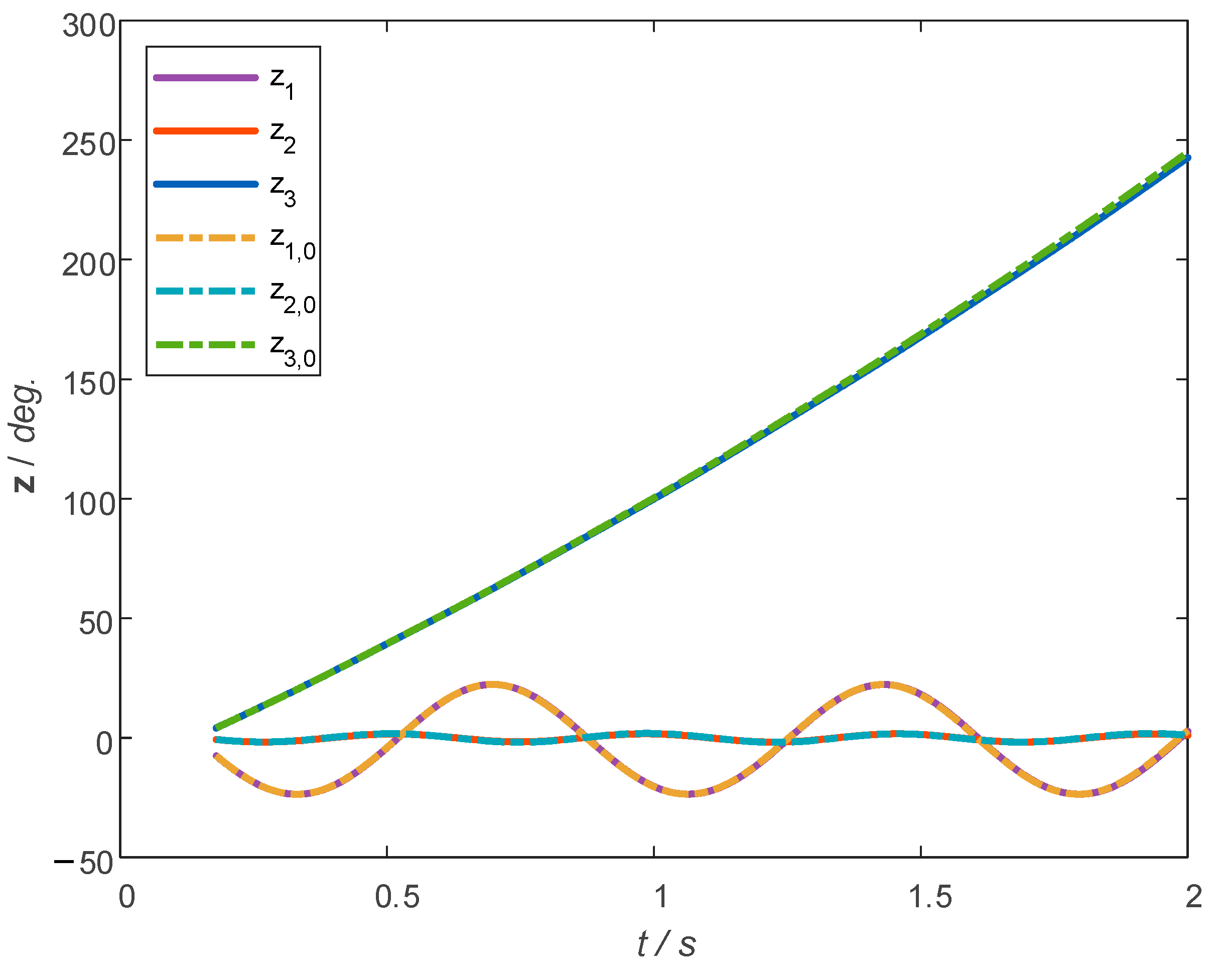
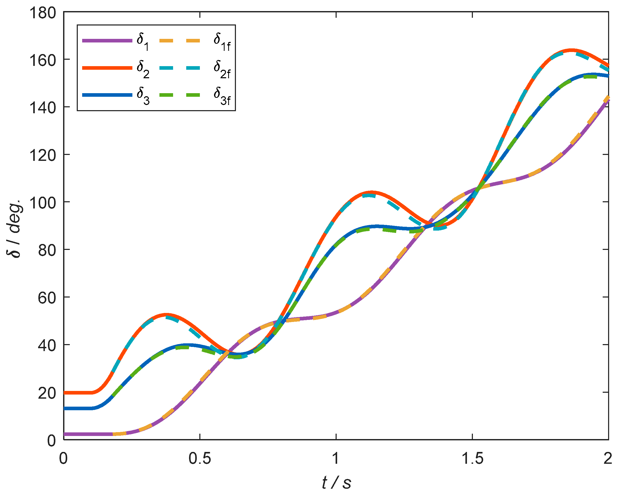
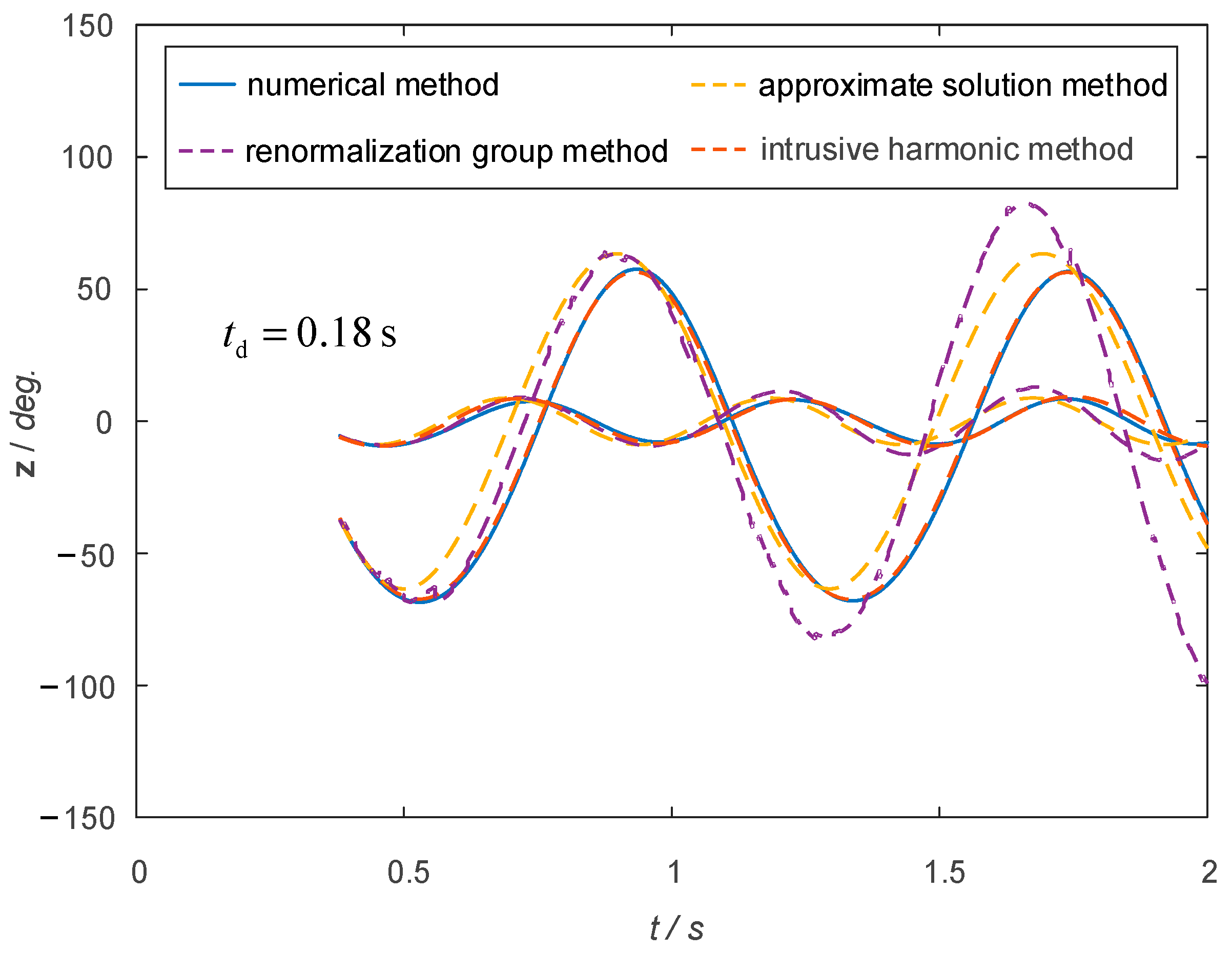
4.1. IEEE Three-Machine Nine-Bus Power System

The topology of the IEEE three-machine nine-bus system example is shown in Figure 2, and the system parameters are referred to in [26] and shown in

Table 1. The parameters of the IEEE 3-machine 9-bus power system.

Generator	$\mathit{\mathscr{H}}$	D	X’d	Xq
G1	23.64	0	0.0608	0.0969
G2	6.40	0	0.1198	0.8645
G3	3.01	0	0.1813	1.2578

.

At 0.1 s, a three-phase short-circuit-to-ground fault is applied at node 7, which lasts for three cycles. After the fault, a continuous fault clearance method is adopted. The original spatial rotor angle response curve of the system is shown in Figure 3 below.

First, observe the rotor angle state of the system during the fault. The rotor angle response during the fault process and the approximate solution of the system are shown in Figure 4 below.

In Figure 4, ${\delta }_{1\mathrm{f}}$ represents the approximate solution of the system during the fault, and other symbols are similar. It can be seen that for the system during the fault, the linear approximate solution well represents the dynamics of the system. According to the calculation, the expression for the linear approximate solution is given by Equation (50), and the unit in the equation is in radians (rad):

$$\left[\begin{array}{c}{\delta }_{1\mathrm{f}}\\ {\delta }_{2\mathrm{f}}\\ {\delta }_{3\mathrm{f}}\end{array}\right]=\left[\begin{array}{l}1.85{(t-0.1)}^2+0.07\cos 6.80(t-0.1)-0.03\\ 1.87{(t-0.1)}^2-0.55\cos 6.80(t-0.1)+0.89\\ 24.00{(t-0.1)}^2+0.23\end{array}\right]$$

(50)

The approximate solution of the system during the fault consists of a quadratic component, a constant component, and an oscillatory component. This corresponds to the breakdown of system responses into a quadratic component ${\mathit{U}}_1{\mathit{J}}_1{t}^2$, a constant component ${\mathit{U}}_2{\left({\mathit{\lambda }}_2^2\right)}^{-1}{\mathit{J}}_2$, and an oscillatory component $-{\mathit{U}}_{2}diag\left(\cos ({\mathit{\lambda }}_{2}t)\right){({\mathit{\lambda }}_2^2)}^{-1}{\mathit{J}}_2$, as proposed in Section 2. The dominance of the quadratic component is evident from the amplitudes of the response components, indicating that the primary response of the system’s power angle to the fault exhibits a quadratic correlation with respect to time. This further substantiates the validity of the analyses previously discussed. Further observing the state of the power system after the fault process, the rotor angle response and approximate transient stability solution in z-space are shown in Figure 5.

In Figure 5, it can be seen that for the system after the fault, the rotor angle response in z-space can be decoupled into synchronous motion components and harmonic motion components, indicating the effectiveness of the previous theoretical analysis. In z-space, the analytical expressions for each component are given by Equation (51):

$$\left[\begin{array}{l}{z}_{1,0}\\ z_{2,0}\\ z_{3,0}\end{array}\right]=\left[\begin{array}{l}23.06\sin \left( 8.708T_0-0.1375T_1+3.423\right)\\ 1.794\sin \left(13.399T_0-0.1293T_1-2.803\right)\\ 14.74T_0^2\hspace{0.17em}+105.40T_1+4.08\end{array}\right]$$

(51)

where $T_0=t_0-0.18\hspace{0.17em},\hspace{0.17em}\hspace{0.17em}{T}_1=t_1-0.18\hspace{0.17em},\hspace{0.17em}\hspace{0.17em}t\ge 0.18$. Furthermore, the analytical solution curves during and after the fault can be transformed into the original rotor angle space, as shown in Figure 6 below.

Figure 6 shows that in the original rotor angle space δ coordinate system, the perturbation solution of the system after the fault can approximate the original rotor angle response curve well, demonstrating the effectiveness of the method and theory presented in this paper.

Furthermore, due to the high analytical capability of the IEEE three-machine nine-bus system, we conducted a comparative study of the approximate solution method, renormalization group method, intrusive harmonic method, and numerical method. At 0.2 s, a three-phase short-circuit ground fault was applied at bus 7, with fault durations set to four and nine cycles, respectively. The comparison of system rotor angle responses obtained from different methods is illustrated in Figure 7 and Figure 8.

As observed in Figure 7 and Figure 8, when the fault duration is relatively short, the system remains in a weakly nonlinear state, and the performance accuracy of the approximate solution method, renormalization group method, and intrusive harmonic method are nearly identical, aligning well with the actual response. However, when the fault duration extends to 0.18 s, the renormalization group method tends to exhibit divergent oscillations, while the other methods continue to fit the rotor angle response relatively well. This suggests that as the fault duration increases and the rotor angle swings into a strongly nonlinear region, the applicability of the methods becomes less reliable.

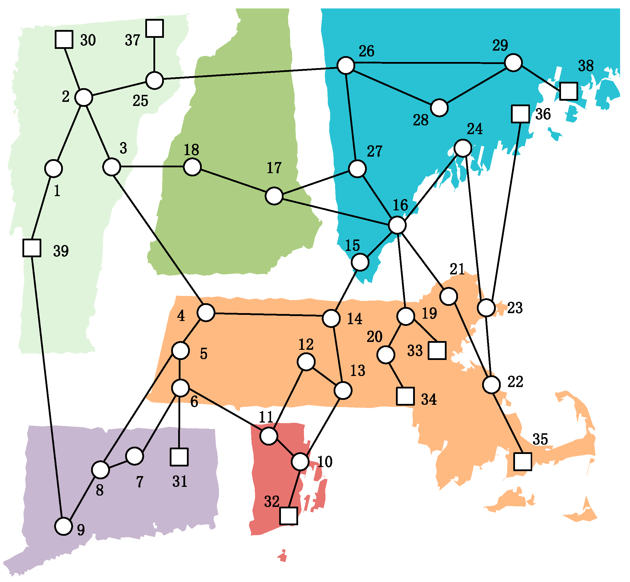
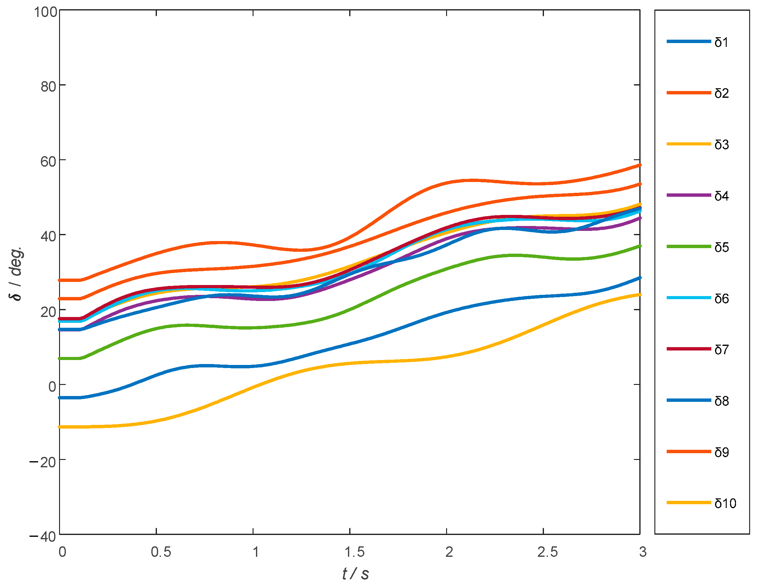
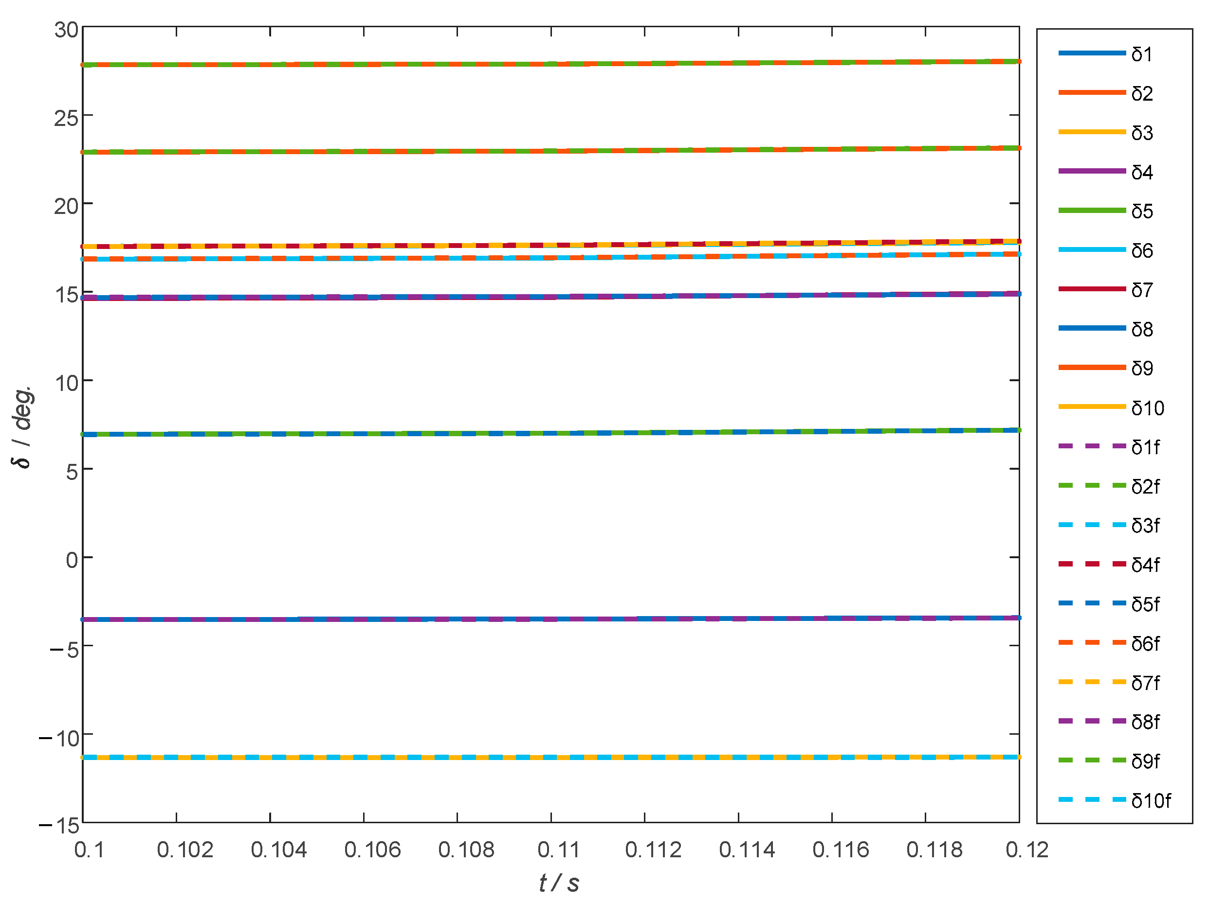
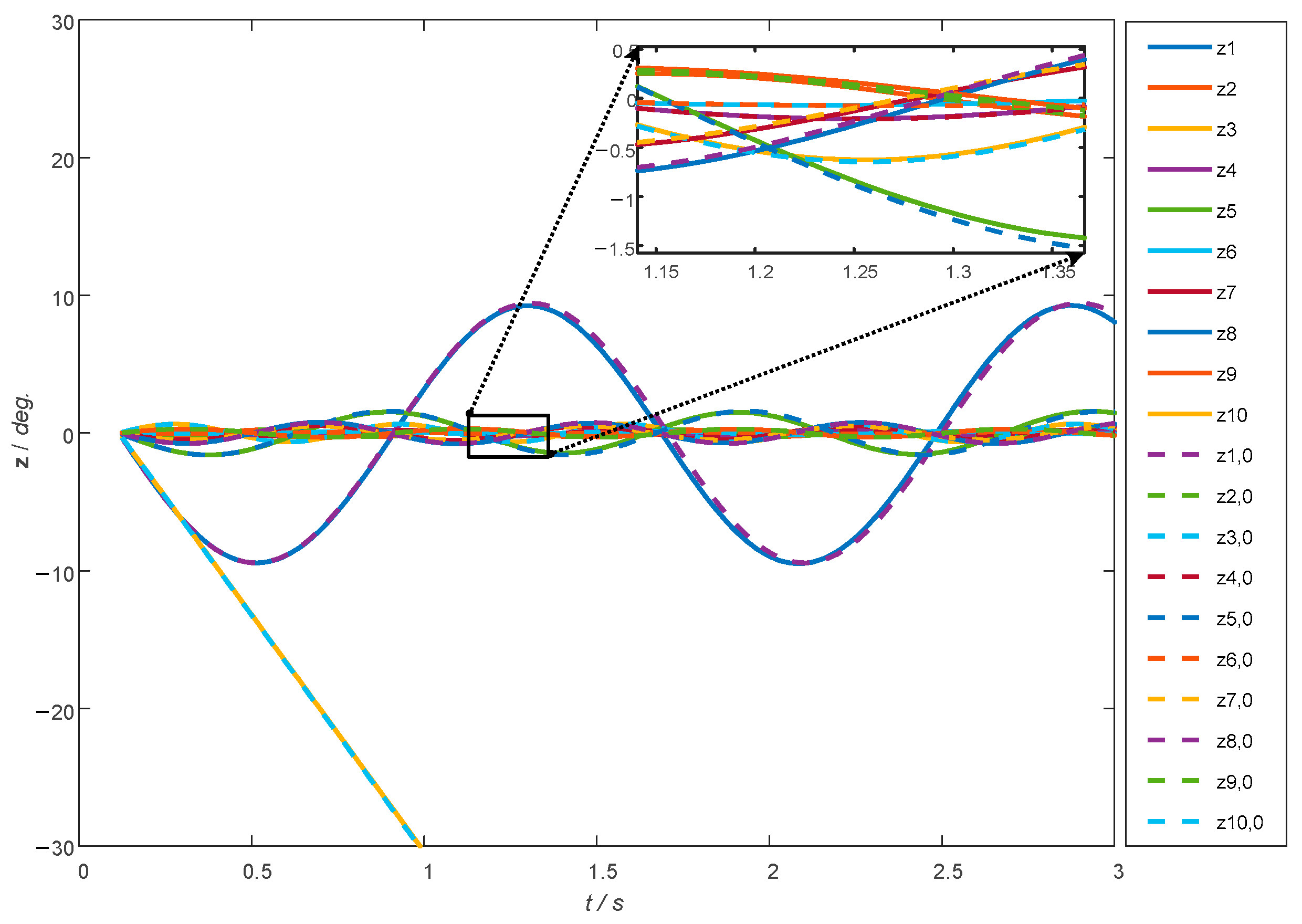
4.2. IEEE 10-Machine 39-Bus Power System

The topology of the IEEE 10-machine 39-bus system is illustrated in Figure 9, with the system parameters provided in reference [27].

At 0.1 s, a three-phase short-circuit ground fault is applied at node 15, which persists for two cycles before employing a continuous fault recovery method. The original spatial rotor angle response curves of the system are illustrated in Figure 10.

In Figure 10, curves of different colors describe the changes in rotor angle response for all units. Upon examining the system during the fault process, the comparative curves of the approximate solution and the original rotor angle response are presented in Figure 11.

In Figure 11, dashed lines represent the approximate solution curves, while solid lines represent the actual response. ${\delta }_{1\mathrm{f}}$ represents the approximate solution of the system during the fault in δ space, and other symbols are similar. It can be observed that the approximate solution curves closely fit the actual response. Furthermore, the response curves of the system after the fault and the approximate solution curves are depicted in Figure 12.

In Figure 12, dashed lines represent the approximate solution curves, and solid lines represent the actual response. $z_{1,0}$ represents the approximate solution after the fault in z-space, and other symbols are similar. A section of the curve is magnified to show details. It is evident that the approximate solution curves closely match the actual response. The transformation of the aforementioned curves from the z-space into the original rotor angle space is shown in Figure 13.

Figure 13 demonstrates that in the original rotor angle space δ coordinate system, the approximate solution curves closely match the actual response, indicating the effectiveness of the method. Furthermore, for different fault-clearing times, the rotor angle oscillation amplitudes in z-space exhibit a monotonic change with increasing clearing time, as depicted in Figure 14.

In Figure 14, $t_{c1}=0.05 \mathrm{s}$, $t_{c2}=0.06 \mathrm{s}$, $t_{c3}=0.07 \mathrm{s}$, and $t_{c4}=0.08 \mathrm{s}$. As the fault-clearing time increases, the rotor angle amplitude shows a monotonically positive relationship with the fault-clearing time. In practical engineering, faults should be cleared as quickly as possible to prevent excessive rotor angle oscillations, which may affect the safe and stable operation of the power system.

5. Conclusions

In this paper, an approximate solution method for transient stability in power systems considering the fault process has been developed and analyzed. By leveraging the sinusoidal coupling characteristics inherent in power system swing equations and applying the Taylor series expansion, we construct a generalized matrix description that reveals the polynomial structural properties of transient stability in power systems. The adoption of coordinate transformation, canonical perturbation techniques, and dual time scales allows us to derive approximate solutions during and after faults, which are shown to effectively describe the dynamic behavior of power systems under significant disturbances.

The significance of this research lies in its ability to provide a deeper mathematical understanding of transient stability phenomena, thereby offering a robust analytical foundation for evaluating and improving power system stability. The polynomial model and the associated approximate solutions contribute valuable insights into the dynamic characteristics of modern power grids, especially in scenarios involving the large-scale integration of renewable energy sources and complex fault processes. The proposed method not only enhances the accuracy of stability analysis but also reduces computational complexity, making it a practical tool for real-time stability assessment in power systems.

Future research directions could focus on extending the proposed methodology to more complex power system models, including those with higher dimensions and more intricate nonlinear dynamics. Additionally, exploring the applicability of the developed techniques to other stability-related issues, such as voltage stability and frequency stability, could provide a more comprehensive framework for power system analysis. Investigating the integration of this analytical approach with advanced numerical simulation techniques might also offer new pathways for improving the accuracy and efficiency of stability assessments in increasingly complex power grids.

References

1. Mochamad, R.F.; Preece, R. Assessing the impact of VSC-HVDC on the interdependency of power system dynamic performance in uncertain mixed AC/DC systems. IEEE Trans. Power Syst. 2019, 35, 63–74. [Google Scholar] [CrossRef]
2. Machowski, J.; Lubosny, Z.; Bialek, J.W. Power System Dynamics: Stability and Control; John Wiley & Sons: Hoboken, NJ, USA, 2020. [Google Scholar]
3. Ma, R.; Zhang, Y.; Yang, Z. Synchronization stability of power-grid-tied converters. Chaos 2023, 33, 032102. [Google Scholar] [CrossRef] [PubMed]
4. Touzé, C.; Vizzaccaro, A.; Thomas, O. Model order reduction methods for geometrically nonlinear structures: A review of nonlinear techniques. Nonlinear Dyn. 2021, 105, 1141–1190. [Google Scholar] [CrossRef]
5. Saha, S.; Vittal, V.; Kliemann, W. Local approximation of stability boundary of a power system using the real normal form of vector fields. In Proceedings of the 1995 IEEE International Symposium on Circuits and Systems (ISCAS), Seattle, WA, USA, 30 April–3 May 1995; Volume 3, pp. 2330–2333. [Google Scholar]
6. Saha, S.; Fouad, A.A.; Kliemann, W.H. Stability boundary approximation of a power system using the real normal form of vector fields. IEEE Trans. Power Syst. 1997, 12, 797–802. [Google Scholar] [CrossRef]
7. Eftekharnejad, S.; Vittal, V.; Heydt, G.T. Impact of increased penetration of photovoltaic generation on power systems. IEEE Trans. Power Syst. 2012, 28, 893–901. [Google Scholar] [CrossRef]
8. Hatziargyriou, N.; Milanovic, J.; Rahmann, C. Definition and classification of power system stability–revisited & extended. IEEE Trans. Power Syst. 2020, 36, 3271–3281. [Google Scholar]
9. Qi, R. Investigation and Visualization of the Stability Boundary for Stressed Power Systems; Iowa State University: Ames, IA, USA, 1999. [Google Scholar]
10. Jiang, L.; Wu, Q.H.; Wang, J. Robust observer-based nonlinear control of multimachine power systems. IEE Proc. Gener. Transm. Distrib. 2001, 148, 623–631. [Google Scholar] [CrossRef]
11. Li, Y.; Zhang, B.; Li, M. Study on Electrical Power System Stability Boundary. Proc. CSEE 2002, 22, 73–78. [Google Scholar]
12. Cheng, D.; Hu, X.; Shen, T. Analysis and Design of Nonlinear Control Systems; Science Press: Alexandria, NSW, Australia, 2010. [Google Scholar]
13. Xue, A.C.; Mei, S.W. Critical clearing time estimation of power system based on quadratic approximation of stability region. Autom. Electr. Power Syst. 2005, 29, 19–24. [Google Scholar]
14. Liu, F.; Wei, W.; Mei, S.W. On expansion of estimated stability region: Theory, methodology, and application to power systems. Sci. China Technol. Sci. 2011, 54, 1394–1406. [Google Scholar] [CrossRef]
15. Qiu, Q.; Ma, R.; Kurths, J. Swing equation in power systems: Approximate analytical solution and bifurcation curve estimate. Chaos 2020, 30, 013113. [Google Scholar] [CrossRef] [PubMed]
16. Liu, Y.; Sun, K. Solving power system differential algebraic equations using differential transformation. IEEE Trans. Power Syst. 2019, 35, 2289–2299. [Google Scholar] [CrossRef]
17. Gurrala, G.; Joseph, F.C. Application of Homotopy Methods in Power Systems Simulations. In Power System Simulation Using Semi-Analytical Methods; John Wiley & Sons, Inc.: Hoboken, NJ, USA, 2023; pp. 197–238. [Google Scholar] [CrossRef]
18. Zhang, W.; Hu, H.L.; Qian, Y.H. A refined asymptotic perturbation method for nonlinear dynamical systems. Arch. Appl. Mech. 2014, 84, 591–606. [Google Scholar] [CrossRef]
19. Wang, F.; Bajaj, A.K. On the Formal Equivalence of Normal Form Theory and the Method of Multiple Time Scales. J. Comput. Nonlinear Dyn. 2009, 4, 021005. [Google Scholar] [CrossRef]
20. Rega, G. Nonlinear dynamics in mechanics and engineering: 40 years of developments and Ali H. Nayfeh’s legacy. Nonlinear Dyn. 2020, 99, 11–34. [Google Scholar] [CrossRef]
21. Krutii, Y.; Vasiliev, A. Development of the Analytical Method of the General Mathieu Equation Solution. East.-Eur. J. Enterp. Technol. 2018, 4, 19–26. [Google Scholar] [CrossRef]
22. Awrejcewicz, J.; Starosta, R.; Sypniewska-Kamińska, G. Asymptotic analysis of resonances in nonlinear vibrations of the 3-dof pendulum. Differ. Equ. Dyn. Syst. 2013, 21, 123–140. [Google Scholar] [CrossRef]
23. Sigamani, V.; Miller, J.J.H.; Narasimhan, R. Differential Equations and Numerical Analysis; Springer: New Delhi, India, 2015. [Google Scholar]
24. Zhang, Q.; Gan, D. A Gronwall Inequality Based Approach to Transient Stability Assessment for Power Grids. arXiv 2023, arXiv:2311.02231. [Google Scholar]
25. Luongo, A.; Zulli, D. Dynamic analysis of externally excited NES-controlled systems via a mixed Multiple Scale/Harmonic Balance algorithm. Nonlinear Dyn. 2012, 70, 2049–2061. [Google Scholar] [CrossRef]
26. Vittal, V.; McCalley, J.D.; Anderson, P.M. Power System Control and Stability; John Wiley & Sons: Hoboken, NJ, USA, 2019. [Google Scholar]
27. Fouad, A.A.; Vittal, V. Power System Transient Stability Analysis Using the Transient Energy Function Method; Prentice Hall: Englewood Cliffs, NJ, USA, 1991. [Google Scholar]
Figure 1. Diagram of the Kuramoto oscillator network.
Mathematics 12 03065 g001
Figure 2. Diagram of IEEE 3-machine 9-bus power system [26].
Mathematics 12 03065 g002
Figure 3. The power angle response of IEEE 3-machine 9-bus system in δ space.
Mathematics 12 03065 g003
Figure 4. The approximate solution of IEEE 3-machine 9-bus system during fault in δ space.
Mathematics 12 03065 g004
Figure 5. The approximate solution of IEEE 3-machine 9-bus system after fault in z-space.
Mathematics 12 03065 g005
Figure 6. The approximate solution of IEEE 3-machine 9-bus system after fault in δ space.
Mathematics 12 03065 g006
Figure 7. A comparison of different methods for a fault duration of 4 cycles.
Mathematics 12 03065 g007
Figure 8. A comparison of different methods for a fault duration of 9 cycles.
Mathematics 12 03065 g008
Figure 9. Diagram of IEEE 10-machine 39-bus power system.
Mathematics 12 03065 g009
Figure 10. The power angle response of IEEE 10-machine 39-bus system in δ space.
Mathematics 12 03065 g010
Figure 11. The approximate solution of IEEE 10-machine 39-bus system during fault in δ space.
Mathematics 12 03065 g011
Figure 12. The approximate solution of IEEE 10-machine 39-bus system after fault in z-space.
Mathematics 12 03065 g012
Figure 13. The approximate solution of IEEE 10-machine 39-bus system after fault in δ space.
Mathematics 12 03065 g013
Figure 14. The effect of the fault clearance time on the power angle oscillation.
Mathematics 12 03065 g014