Hybrid Deep Neural Network Approaches for Power Quality Analysis in Electric Arc Furnaces

Abstract

In this research, we investigate the power quality of the grid where an Electric Arc Furnace (EAF) with a very high load operates. An Electric Arc Furnace (EAF) is a highly nonlinear load that uses very high and variable currents, causing major power quality issues such as voltage sags, flickers, and harmonic distortions. These disturbances produce electrical grid instability, affect the operation of other equipment, and require strong mitigation measures to reduce their impact. To investigate these issues, data are collected from the Point of Common Coupling where the Electric Arc Furnace is fed. The following three main factors are identified for evaluating power quality: apparent power, active and reactive power, and distorted power. Along with these powers, Total Harmonic Distortion, an important indicator of power quality, is calculated. These data are collected during the full process of producing a complete steel batch. To create a Deep Neural Network that can model and forecast power quality parameters, a network is developed using LSTM layers, Convolutional Layers, and GRU Layers, all of which demonstrate good prediction performance. The results of the prediction models are examined, as well as the primary metrics characterizing the prediction, using the following: MAE, RMSE, R-squared, and sMAPE. Predicting active and reactive power and Total Harmonic Distortion (THD) proves useful for anticipating power quality problems in an Electric Arc Furnace (EAF). By reducing the EAF’s impact on the power system, accurate predictions will anticipate and minimize disturbances, optimize energy consumption, and improve grid stability. This research’s principal scientific contribution is the development of a hybrid deep neural network that integrates Convolutional Neural Networks (CNNs), Long Short-Term Memory (LSTM), and Gated Recurrent Unit (GRU) layers. This deep neural network was designed to predict power quality metrics, including active power, reactive power, distortion power, and Total Harmonic Distortion (THD). The proposed methodology indicates an important step in improving the accuracy of power quality forecasting for Electric Arc Furnaces (EAFs). The hybrid model’s ability for analyzing both time-series data and complex nonlinear patterns improves its predictive accuracy compared to traditional methods.

1. Introduction

Electric Arc Furnaces (EAFs) are extensively utilized in the steel manufacturing industry to melt scrap steel by employing a high level of electric arcs. Electric arc furnaces (EAFs) play an important part with regard to efficient steel production. However, their nonlinear and variable load characteristics have a substantial effect on power quality [1,2,3,4,5]. Currently, the power quality of the electrical energy that is given to customers is one of the most significant global concerns. An electric arc furnace is one of the consumers that negatively affects load asymmetry [5], harmonics introduced into the network, and reactive power circulation [3,4]. The aim of this study is to investigate potential solutions that might be employed to mitigate the unfavorable effects generated by the installation of the electric arc furnace.

The EAFs are responsible for a substantial amount of reactive power, which is one of the most major negative consequences they cause. Both the distribution network and the overall efficiency of the power supply system could be impacted as a result of this, which may cause the distribution network to become overloaded [5]. Reactive power is one of the most significant problems related to the functioning of electric arc furnaces (EAFs) and has a number of negative impacts on power quality. Electric arc furnaces have a low power factor due to their high reactive power values. A low power factor results in energy inefficiency, since more energy must be generated and transferred to meet the same need for active power [3]. The primary source of reactive power is that EAF is a nonlinear load. Current and voltage imbalances between the three phases of the electrical grid are the result of EAFs; these imbalances may interfere with the functionality of other equipment that are connected to the same grid [4]. Electric Arc Furnaces use the electric arc for melting the scrap [2,5]. The electric arc is nonlinear and produces higher order harmonics in the network’s current and voltage. Harmonic orders are multiples of the fundamental frequency, for example, harmonics of order 3, 5, 7, and so on [6]. Harmonics produce distortions in the voltage and current waveforms, affecting the functioning of electronic equipment. Harmonics can interact with inductive and capacitive elements in the power network, creating resonance phenomena that can result in equipment overload and failures [1]. The rapid and frequent fluctuations of electric current caused by EAFs result in voltage variations (flicker) in the power grid. These fluctuations in voltage are seen as flickering lights and can be inconvenient for consumers [1,2].

These EAFs have the potential to affect the electrical grid by causing load asymmetry, which in turn results in voltage and current imbalances. The imbalances can have a negative impact on other components of equipment that are connected to the same network, which can result in damage to the equipment as well as an increase in the amount of network losses [7].

This paper aims to study possible solutions to limit the negative effects caused by the electrical installation of the electric arc furnace. To conduct a comprehensive study, measurements were taken in the power supply installation of the three-phase electric arc furnace, both in the primary and secondary of this transformer.

Thus, the paper is structured as follows:

The “Related Works” section presents other research that addresses the issues caused by EAFs.

The “Materials and Methods” section presents measurements from the PCC (Point of Common Coupling), which were obtained during the actual installation of an EAF, as well as the main power quality indicators. This section also includes a hybrid Deep Neural Network designed for modeling and predicting the main indicators of power quality.

The “Results” part displays the modeling results, while the “Discussion” section evaluates the quality of the developed models using the primary prediction metrics like RMSE (Root Mean Square Error), MAE (Mean Absolute Error), R2-squared (coefficient of Determination), and sMAPE (Symmetric Mean Absolute Percentage Error).

2. Related Works

Numerous studies have been conducted to investigate the implications of an EAF on the electrical system, as well as approaches that can be implemented to mitigate these effects. In this section, some of these research studies are presented.

A multiple synchronous reference frame (MSRF) analysis framework is used in [1] to determine the positive and negative sequence components of interharmonic and harmonic currents from AC EAF installations. The MSRF analysis uses continuously measured line currents and voltages on the medium-voltage side of the EAF transformer at 25.6 KHz per data channel to characterize interharmonics and harmonics online. Offline computations reveal that the proposed framework’s compensation of sequence components of interharmonics and harmonics of EAF currents reduces short-term flicker values at the site of common coupling by up to 10-fold. The MSRF analysis framework was validated by comparing EAF current frequency spectrums to Fourier analysis results using 10-cycle sliding windows.

The article [2] discusses the conceptual problems of the method to determine the static var compensator (SVC) minimum power level in the steel-making electric arc furnace’s electric power supply system. The complex shaft furnace (SF-150) and SVC of CJSC Severstal–Balakovo light-section rolling mill and EAF-120-SVC of PJSC Asha metallurgical plant were simulated for the research. The study group compared the results and calculated the static var compensator power levels to balance the asymmetrical load in most EAF operation modes.

According to [3], the ZHD (Zero Harmonic Distortion Converter) converter static synchronous compensator (STATCOM) can increase the displacement power factor of an electric arc furnace (EAF) application from 0.88 to 0.98, with total demand distortion in the grid around 1.44%. This result is achieved without using high-order sinusoidal filters and with consolidated components in the industry.

The enhanced time-domain EAF model [4] used DSP-based MC (Matrix Converter) and SVC. The proposed model improved system power quality. The results lead to the following conclusions: the highest arc current and voltage are around 123.26 kA and 314 V, respectively. The suggested approach yields the lowest current and voltage THD values of 2.85% and 29.54%, respectively. The proposed model has a minimum voltage flickering scale of 1.26% compared to other models. The power factor of the suggested method is approximately 0.9975, which is superior. These improvements allow the suggested technology to be used in real time, such as in a steel manufacturing plant that provides high-quality electricity and energy efficiency.

Time- and frequency-domain Deep Learning (DL) algorithms were developed to predetect harmonic and interharmonic components of an Electric Arc Furnace (EAF) current waveform [6]. Tests using field data showed accurate prediction of all harmonics up to 50th order and interharmonics with 5 Hz resolution. The proposed system for Active Power Filters (APFs) for harmonics and interharmonics has been tested in a simulation environment using field data and found to be effective.

Many studies are based on electric arc modeling, because the electric arc is highly nonlinear. For EAF modeling and simulation, the research [7] analyzes piece-wise linear, modified piece-wise linear, hyperbolic, exponential, and exponential–hyperbolic time-domain models. Adapting EAF characteristics requires optimal parameter estimates for the introduced models. The data of an actual Iranian EAF-based steel firm validate the proposed method from [7]. Results indicate that the modified piece-wise linear model best predicts EAF behavior. New models based on instantaneous EAF voltage and current from the steel industry in Iran are proposed in paper [8]. This research proposes three modified Schwarz models for efficient modeling. Calculations of active power, harmonics, instantaneous flicker, and short-term flicker evaluate the accuracy of the proposed model from [8]. The optimal model ordering for refining, melting, and scrapping phases are determined in [9] using actual EAF records. The first proposed model uses optimal model ordering with time-varying model parameters, unlike the original power balance equation. In the second model, model orders vary continuously. Every 10 ms, autoregressive moving average (ARMA) models update their parameters. Calculating several important electric values using actual data and the proposed models from [9] verifies their accuracy.

This research [10] provides an optimal electric arc furnace model parameter estimate approach. The methodology from [10] was evaluated using real and simulated data and the following three metaheuristic optimization algorithms: PSO (Particle Swarm Optimisation), VSA (Vortex Search Algorithm), and CSA (Crow Search Algorithm). The study [10] determined that meta-heuristic optimization approaches efficiently estimated the electric arc furnace model parameters in a single optimization step, captured the non-sinusoidal, non-linearity, and time-varying random behavior of real electric arc furnace samples, and obtained relative errors of the total harmonic distortion between the measured and estimated voltage and arc current.

The work [11] addresses estimating EAF model parameters. The method uses a support vector, machine-based, multiple-input, multiple-output regressor to map electric arc voltage characteristics to model parameters. A multidimensional support vector regressor (M-SVR) has been developed in training, utilizing data obtained from various EAF model simulations. The study [11] showed a 2.1% and 6.3% relative errors between the fundamental component of current and voltage for real and simulated waveforms, respectively.

The article [12] investigates methods to improve the Static Var Compensator (SVC) control system to reduce flicker. The SVC control system has an open loop that responds rapidly to dynamic changes in Electric Arc Furnace (EAF) power and a closed loop that provides precision control to guarantee the Point of Common Coupling power factor is met. The proposed techniques from [12] were tested using experimental laboratory equipment and a frequency domain theoretical model. Real-world EAF data were used in a VSC experiment to simulate its dynamic behavior.

The paper [13] proposes to develop two enhanced versions of accurate models based on the Schavemaker model for the electric arc.

In paper [14], arc furnace power factor correction is performed with a mix of active and passive techniques. The target power factor is achieved at 50% of the cost of active devices only. The final results in [14] demonstrate 84.7% EAF reactive power reduction with PF > 0.98. The EAF active consumption of energy increased 16.7%.

In their study [15], the authors present an approach to EAF modeling based on a deterministic differential equation that is improved with stochastic components. A genetic method is used to identify the time series corresponding to equation coefficients. The final solution includes two types of the electric arc furnace, both built on long short-term memory (LSTM) networks.

Deep machine learning-based approaches and a novel data augmentation are used to predict flicker, voltage dip, harmonics, and interharmonics from highly time-varying electric arc furnace (EAF) currents and voltage [16]. The prediction counters the response and reaction time delays of electric arc furnace-specific active power filters (APFs). The MSRF analysis splits out EAF current and voltage waveform frequency components into dqo components. The APF reference signals are created using low-pass filters and dqo component predictions. Three approaches exist. A low-pass Butterworth filter and linear finite impulse response (FIR) or long short-term memory network (LSTM) are utilized in two of them. In the third method from [16], a deep CNN and LSTM network filter and predict simultaneously. The Butterworth and linear prediction, Butterworth and LSTM, and CNN and LSTM approaches yield 2.06%, 0.31%, and 0.99% dqo component prediction errors for a 40 ms prediction horizon, respectively [16]. The predicted waveforms of flicker, harmonics, and interharmonics had 8.5%, 1.90%, and 3.2% reconstruction errors for the given approaches, respectively. A Simulink and GPU-based predictive APF solution using Butterworth filter + LSTM and a simple APF compensated EAF current interharmonics with 96% and 60% efficiency, respectively.

A data-driven compartmental modeling approach (DCMM) for the multi-mode EAF harmonic model is proposed in [17]. The proposed DCMM considers harmonic frequency coupling to increase modeling accuracy and reduces harmonic dataset dimensions to improve computational efficiency. The performance evaluation results [18] demonstrate that the proposed DCMM can create the multi-mode model even if data amounts, cluster numbers, and sample distribution change significantly.

In the study [18], a deep learning (DL)-based method for the fast and accurate analysis of current harmonics in electric arc furnaces (EAF) is proposed. The harmonic nature of EAF current data is derived as statistical distributions using field data collected from transformer substations that power EAF plants at the transmission system level.

The study [19] describes an adaptive neuro-fuzzy system that is used for predicting current through an electric arc furnace. To accomplish this aim, an ANFIS system was trained with measured data from an electric arc furnace installation.

The paper [20] describes a study using an EAF model for determining reactive power levels. The results were obtained by simulating several steps of the reactive power compensation installation with the premise that harmonics filters are connected.

The paper [21] used a model based on the electric arc’s current–voltage characteristics. The simulation results were compared to data obtained by the authors at an industrial plant where a 100 UHP electric arc furnace was functioning.

Generally, previous studies have primarily focused on modeling the Electric Arc, studies on the power quality on the PCC (Point of Common Coupling) where an EAF is connected, as well as methods to predict the power quality issues. This research also focuses on power quality, specifically the possibility of employing deep hybrid neural networks to predict the active power received from the grid by an EAF, allowing the power factor to be as near to the maximum value as possible (power factor = 1). The main scientific contribution of this research is the development of a hybrid deep neural network that integrates Convolutional Neural Networks (CNN), Long Short-Term Memory (LSTM), and Gated Recurrent Unit (GRU) layers. This deep neural network is designed to forecast power quality indicators, including active power, reactive power, distortion power, and Total Harmonic Distortion (THD). The proposed methodology represents significant progress in improving the accuracy of power quality prediction for Electric Arc Furnaces (EAFs). The hybrid model’s ability to analyze both time-series data and complex nonlinear patterns enhances predictive performance compared to conventional methods.

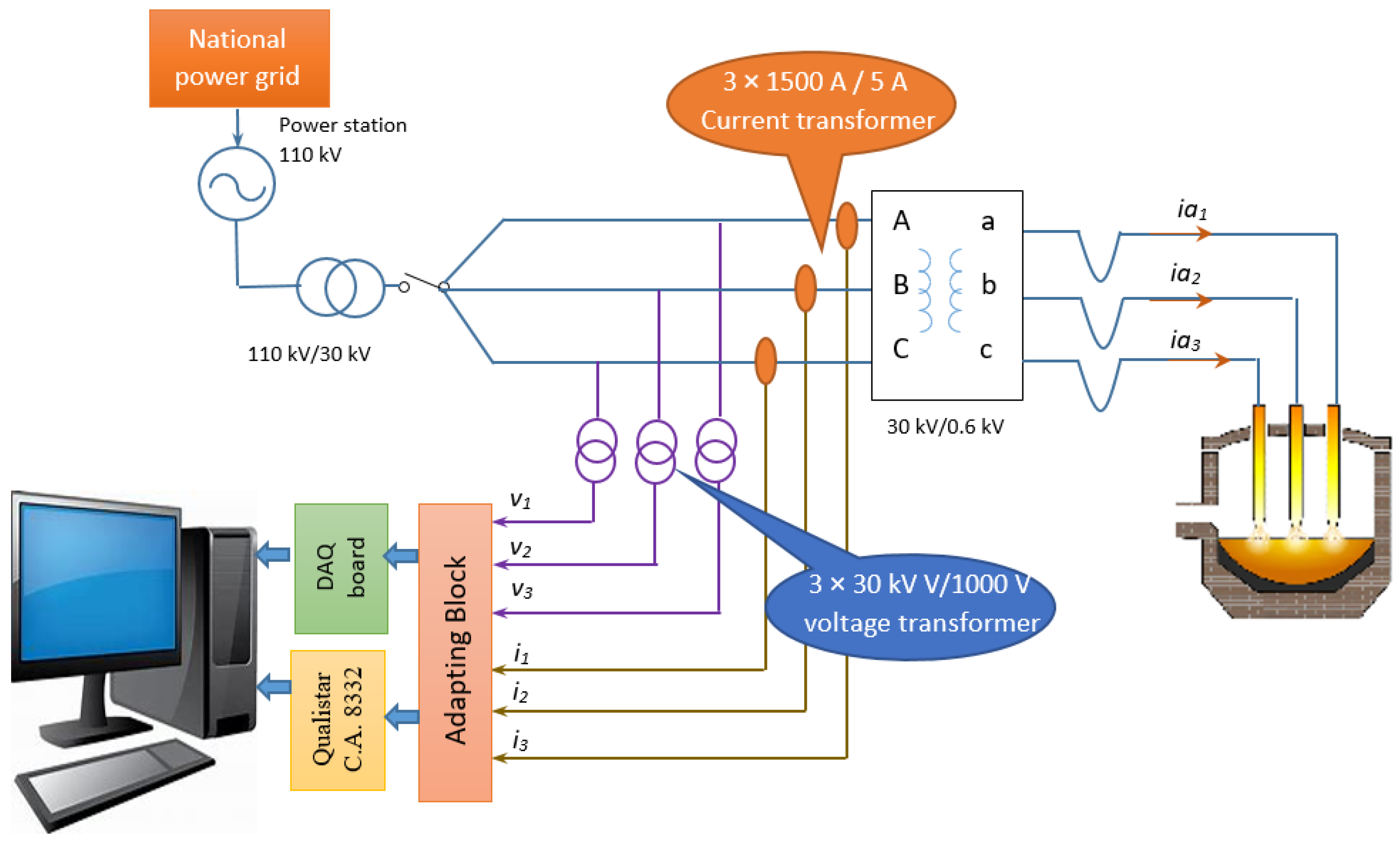
3. Materials and Methods

To investigate the power quality in the electric arc furnace power plant, extensive measurements were taken in the electrical power plant of an electric arc furnace with a capacity of 100 metric tons. Thus, the instantaneous current and voltage values, as well as the active, reactive, and distorted power, were determined. The distorted power is the power produced by harmonics that differ from the fundamental frequency. The THD and power factor data were also calculated.

The electrical measurement scheme is depicted in Figure 1.

Current and voltage measurements are performed using current and voltage transformers, with the secondaries connected to a measurement system. To conduct a study of electrical items over the duration of a steel production process, data were collected throughout the batch.

To measure the voltage on the medium voltage supply line, a voltage transformer with a transformation ratio of 30,000 V/1000 V was used, having measurement errors of 2.5% and a frequency bandwidth of 5 KHz. To measure the current on the medium voltage supply line, a current transformer with a transformation ratio of 1500 A/5 A was used, with a frequency band of 5 KHz and 2.5% measurement errors.

Secondary voltage and current transformers have been connected to a block’s inputs to adjust high voltages and currents. The main characteristics are as follows:

• The voltage measurement channel’s maximum operating frequency is 15 KHz, which matches the cutoff frequency of the isolation amplifier and alternating current amplifier assembly. The nonlinearity error in the voltage measurement process in the 1000 V range is less than 1% in the frequency range of 15 KHz.
• The nonlinearity error in the current measurement process is within 0.5% of the frequency range of the current transducer, which is in the frequency range of 100 KHz.

It has been noticed that the errors introduced by the current and voltage adapting block are less than those introduced by the current and voltage measurement transformers.

The proposed acquisition equipment consists of a laptop and an integrated controller NI MyRIO 1900 (Xilinx processor, FPGA, and Real Time technology, 667 MHz, produced by National Instruments Corporation, Austin, Texas, United States) equipped with FPGA (Field Programmable Gate Array) and Real Time technologies that communicate with a host computer with LabVIEW myRIO 2014 software package.

As shown in Figure 1, the measurement of current and voltage is performed using 3 × 1500 A/5 A current transformers and 3 × 30,000 V/1000 V voltage transformers. Measurements were taken using both an NI MyRIO 1900 and a Qualistar C.A. 8332 (produce by Chauvin Arnoux, Paris, France) power measurement instrument. The software package used with this device was PAT Version 3.05.0032. Because the measured values were very high, a current and voltage adaption block was used to adjust these values to the values accepted by the NI MyRIO 1900 and the Qualistar device. The results of the measurements made with both devices were similar; the main difference is that the NI MyRIO 1900 board allowed for the identification of interharmonics.

Analysis of the transformers’ errors in measurements revealed a 2.5% error rate, which is unavoidable given their integration into the current installation. The error measurements with the NI MyRIO 1900 and Qualistar C.A. 8332 are approximately 1%.

Figure 2 depicts the waveforms of the currents and voltages on the EAF’s power supply line during the melting phase, which show significant distortion. It is also noted that because the amplitudes of the currents and voltages on the three phases are unequal, the load is highly unbalanced. The distortions that appear in the waveforms of the current and voltage are significantly reduced in the stable stage phase of the electric arc, which occurs near the end of the charge development, particularly during the oxidation and reduction (deoxidation) processes, as shown in Figure 3, which depicts the waveforms obtained in the refining phase. In this phase, the amplitudes of currents and voltages are significantly closer in value, indicating that the load impedance is more balanced.

Figure 2a shows voltage variations across all three phases, indicating that the power demand varies significantly during the melting process. These changes are predictable given the nature of melting, which requires intermittent high power to achieve and sustain the required temperatures. The asymmetries in the electrical load or the differences in the electrical characteristics of each phase are the reasons for the differences between phases. Furthermore, the high and fluctuating currents in Figure 2b are representative of the melting stage in an EAF, during which substantial quantities of electrical power are converted to heat. The unbalanced load and variations in the operational conditions of each phase are the causes of the phase-specific differences.

The voltage curves in Figure 3a demonstrate the necessity for more precise and stable control of the power supply during the refining stage. Compared to the melting stage, the refining process involves the fine tuning of the composition and temperature of the liquefied material, rather than the large-scale consumption of energy necessary for melting. This is indicated by the reduced fluctuations.

Balanced and controlled electrical conditions are essential for achieving the desired material properties in the final product, as evidenced by the stability observed in all three phases. Figure 3b shows more uniform current waveforms during the refining stage, indicating the accuracy necessary for controlling the chemical composition and temperature of the molten material.

Compared to the melting phase, the refining process requires less large power changes, resulting in smoother current variations.

3.1. Power Quality Analyze

However, the voltage and current in both stages are not completely sinusoidal. To analyze power quality, measured instantaneous current and voltage values are needed to process the data to calculate voltage and current harmonics, Total Harmonic Distortion (THD), power factor, and other power quality indicators [22].

The following procedure was used to get current and voltage values on the medium voltage line over six channels, three currents, and three voltages:

Data were acquired simultaneously on the six channels during the first time interval, which comprised 250 ms, at a frequency of 5 KHz. In this manner, the signals were acquired over a period of 12.5 periods. Under certain conditions when the supply voltage frequency varies from 50 Hz, the data can include a number of 12 complete cycles, which can be selected through the program.

The data acquisition procedure was repeated, generating a total of 4800 values during the 2.5 h batch processing.

The spectrum characteristics have been calculated by processing the acquired data using the Fourier transform. Since the acquisition frequency was 5 KHz, the frequency band for analysis is 0–2.5 KHz, which is divided by the number of 1250 samples in the data window and provides a frequency range of 2 Hz.

3.1.1. The Power Quality Indicators in the Context on an EAF

Even though PQ indicators are widely recognized, a synthesis of these indicators is provided. In the electrical signal, harmonics are components that occur at various frequencies of the fundamental frequency.

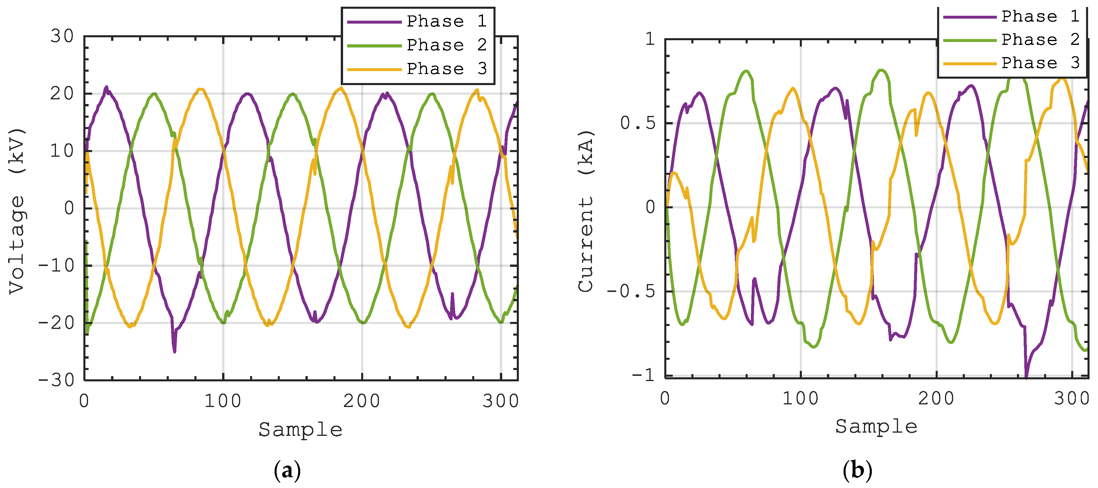
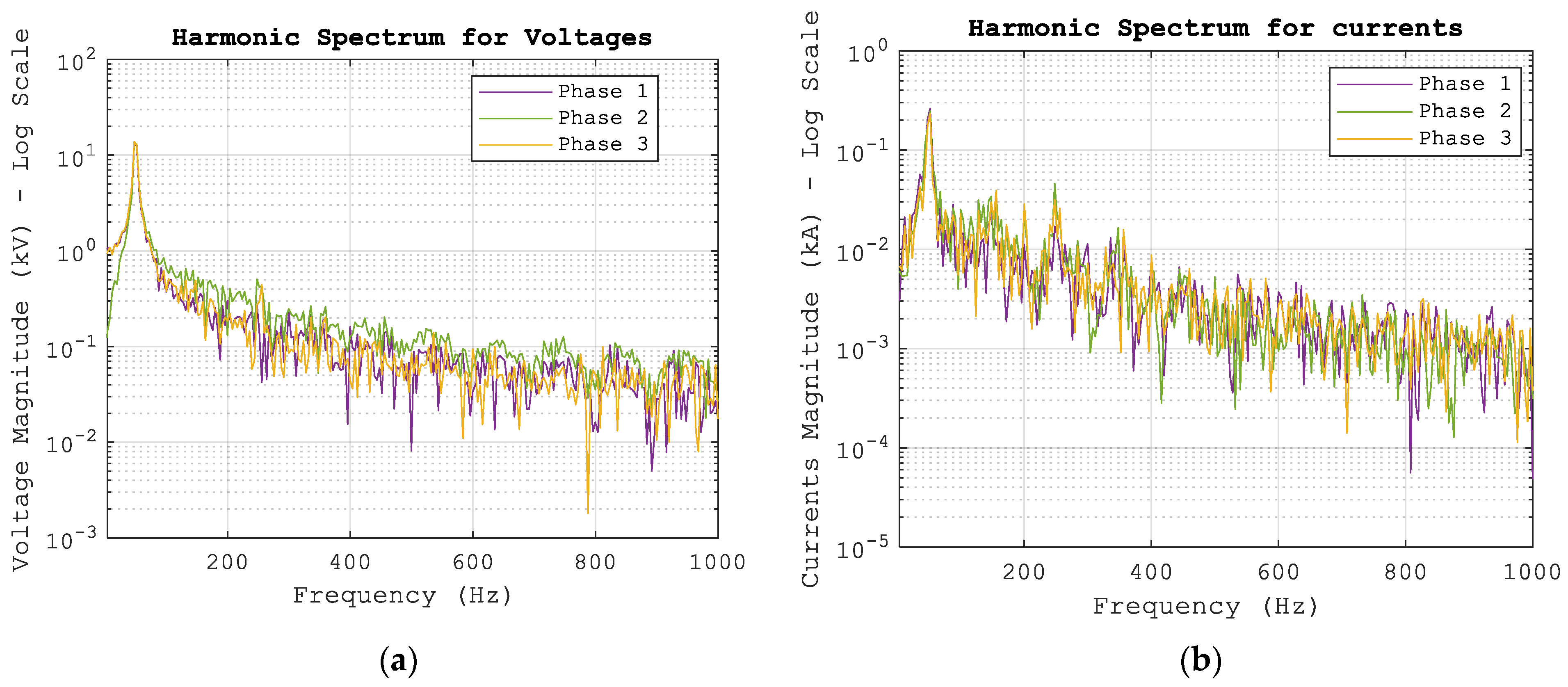
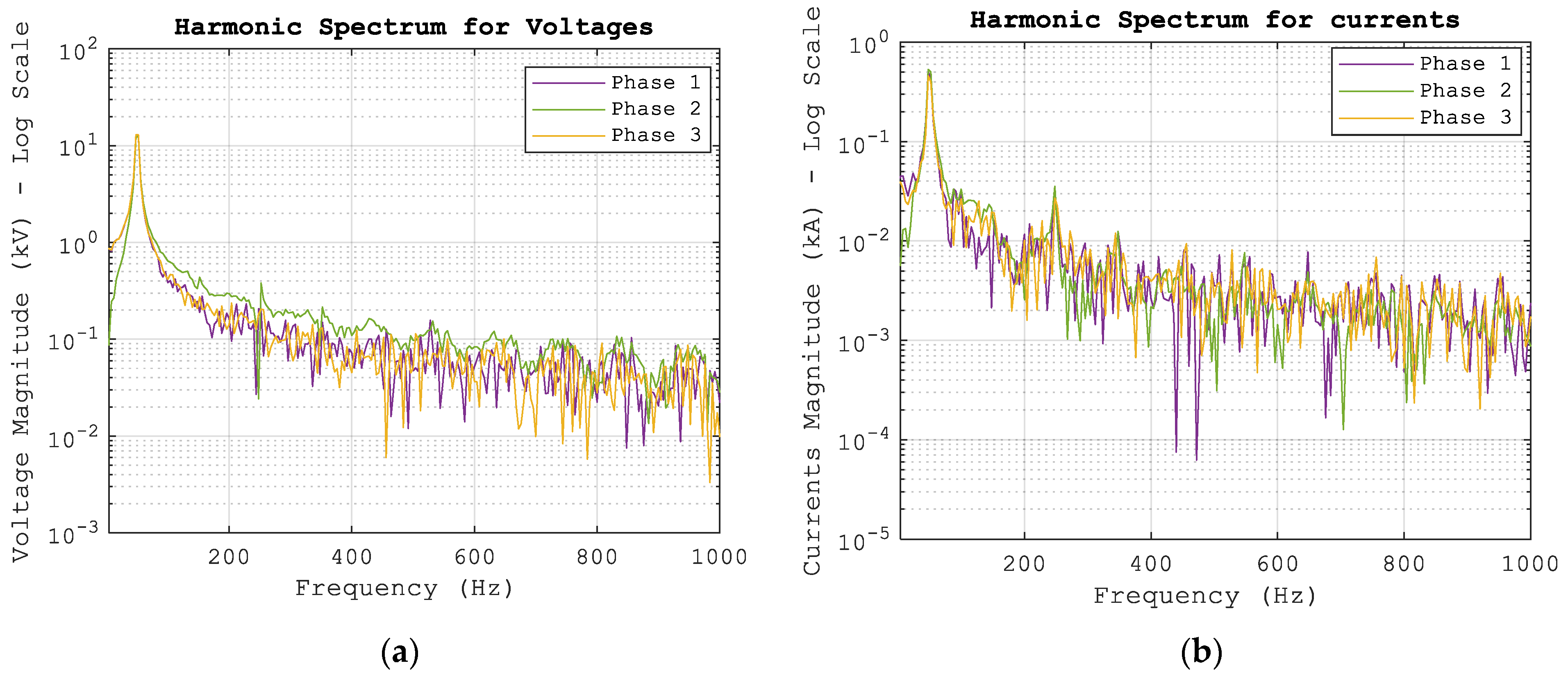
3.1.2. Harmonic Voltage

The harmonic voltage of order n (V_n) can be expressed with the following Equation (1):

$$V_n\left(t\right)=V_{nrms}·\sqrt{2}·cos\left(n\omega t+{\theta }_n\right),$$

(1)

3.1.3. Harmonic Current

The harmonic current can be similarly expressed by the following (2):

$$I_n\left(t\right)=I_{nrms}·\sqrt{2}·cos\left(n\omega t+{\phi }_n\right),$$

(2)

where:

n is the harmonic order (1 for the fundamental, 2 for the first superior harmonic and so on).

The term V_nrms represents the RMS value of the n-order harmonic of the voltage, while I_nrms is the RMS value of the current for the same harmonic.

ω is the angular pulsation of the fundamental frequency (ω = 2πf).

θ_n is the phase angle of the harmonic voltage of order n.

ϕ_n is the phase angle of the harmonic current of order n.

3.1.4. The RMS Voltage

The total RMS voltage ($V_{{total}_{rms}})$ taking harmonics into account can be calculated using the following:

$$V_{{total}_{rms}}=\sqrt{V_{1_{rms}}+V_{2_{rms}}+V_{3_{rms}}+\cdots +V_{n_{rms}}},$$

(3)

where $V_{1_{rms}}$ is RMS value of the fundamental and $V_{n_{rms}}$ are the RMS values of the harmonic components of the voltage.

3.1.5. The RMS Current

The total RMS current ($I_{{total}_{rms}})$ taking harmonics into account can be calculated using the following:

$$I_{{total}_{rms}}=\sqrt{I_{1_{rms}}+I_{2_{rms}}+I_{3_{rms}}+\cdots +I_{n_{rms}}},$$

(4)

where $I_{1_{rms}}$este is RMS value of the fundamental and $I_{n_{rms}}$ are the RMS values of the harmonic components of the voltage.

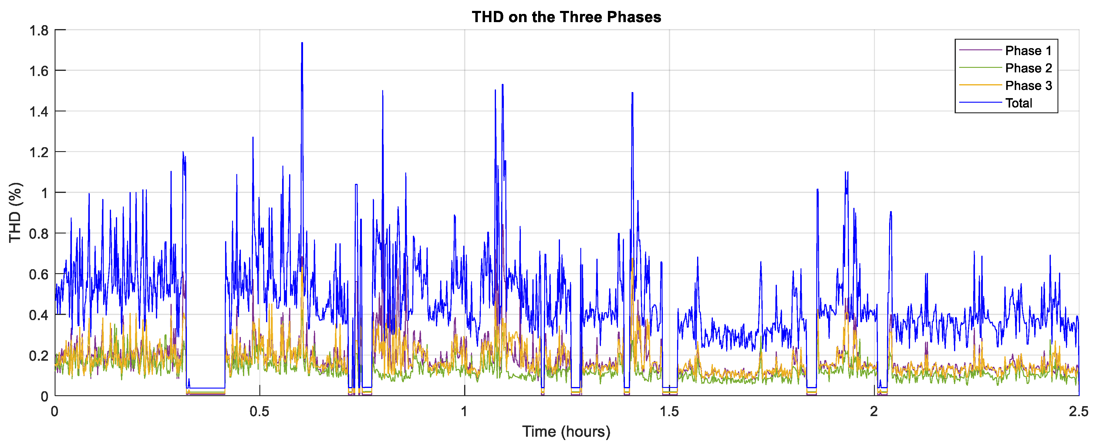
3.1.6. The Total Harmonic Distortion (THD)

The THD for voltage and current can be expressed using the following Equations (5) and (6):

$${THD}_V={\displaystyle \frac{\sqrt{V_{2_{rms}}+V_{3_{rms}}+\cdots +V_{n_{rms}}}}{V_{1_{rms}}}},$$

(5)

$${THD}_I={\displaystyle \frac{\sqrt{I_{2_{rms}}+I_{3_{rms}}+\cdots +I_{n_{rms}}}}{I_{1_{rms}}}},$$

(6)

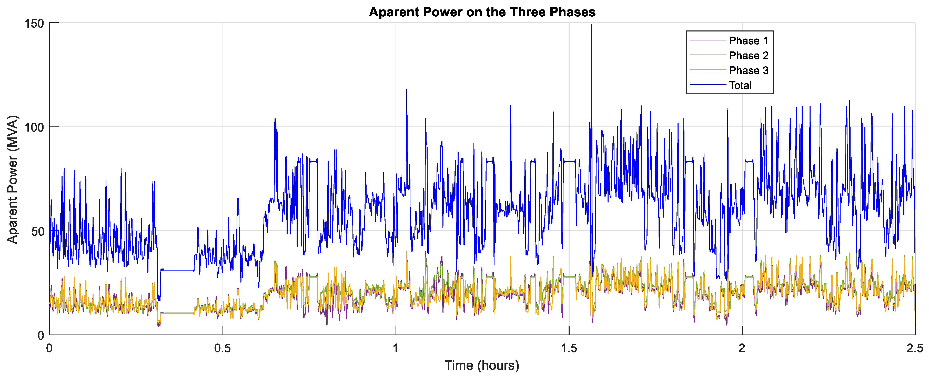
3.1.7. The Apparent Power (S)

The apparent power, S, is given by the product of the RMS voltage (V) and the RMS current (I) as follows:

$$S=V·I,$$

(7)

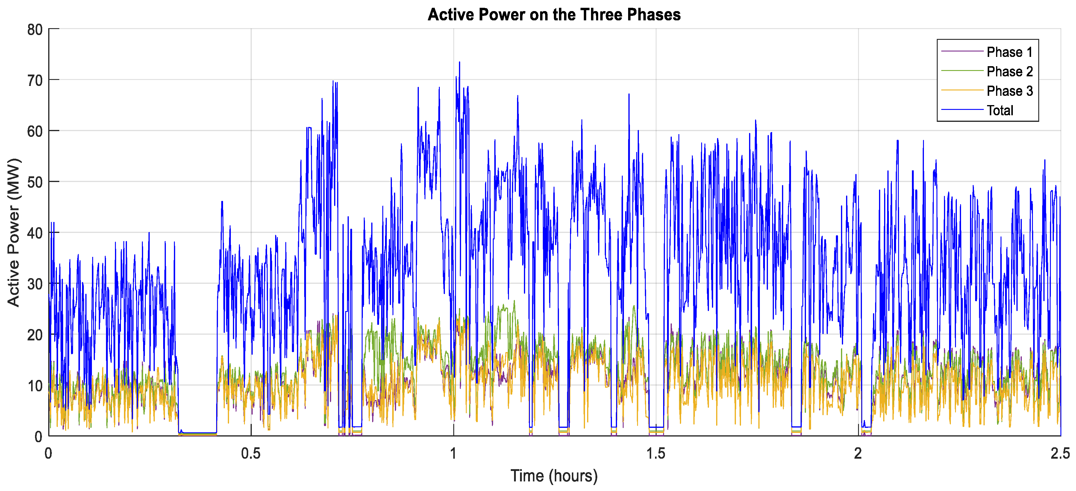
3.1.8. The Active Power (P)

The active power, measured in watts (W), denotes the power that is effectively utilized to melt the load is described as follows:

$$P=V·I·cos\left(\phi \right),$$

(8)

where $cos\left(\phi \right)$ is the phase difference between V and I and also represents the power factor.

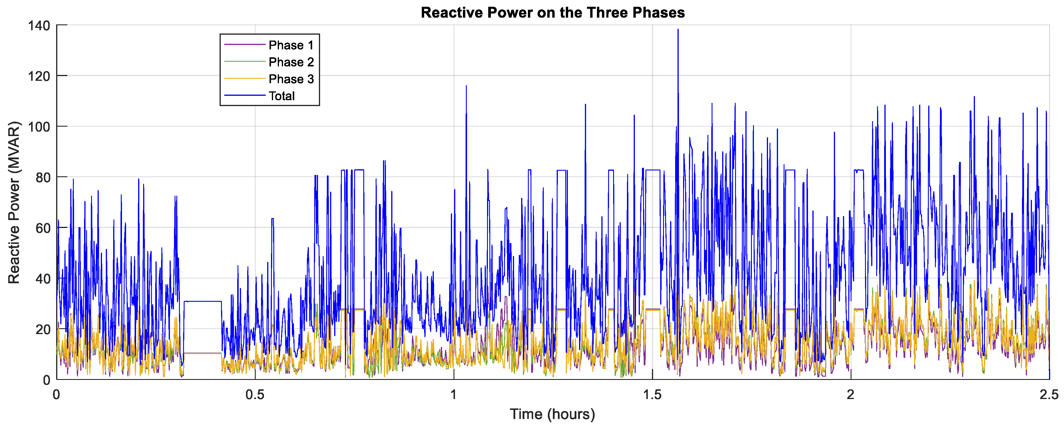
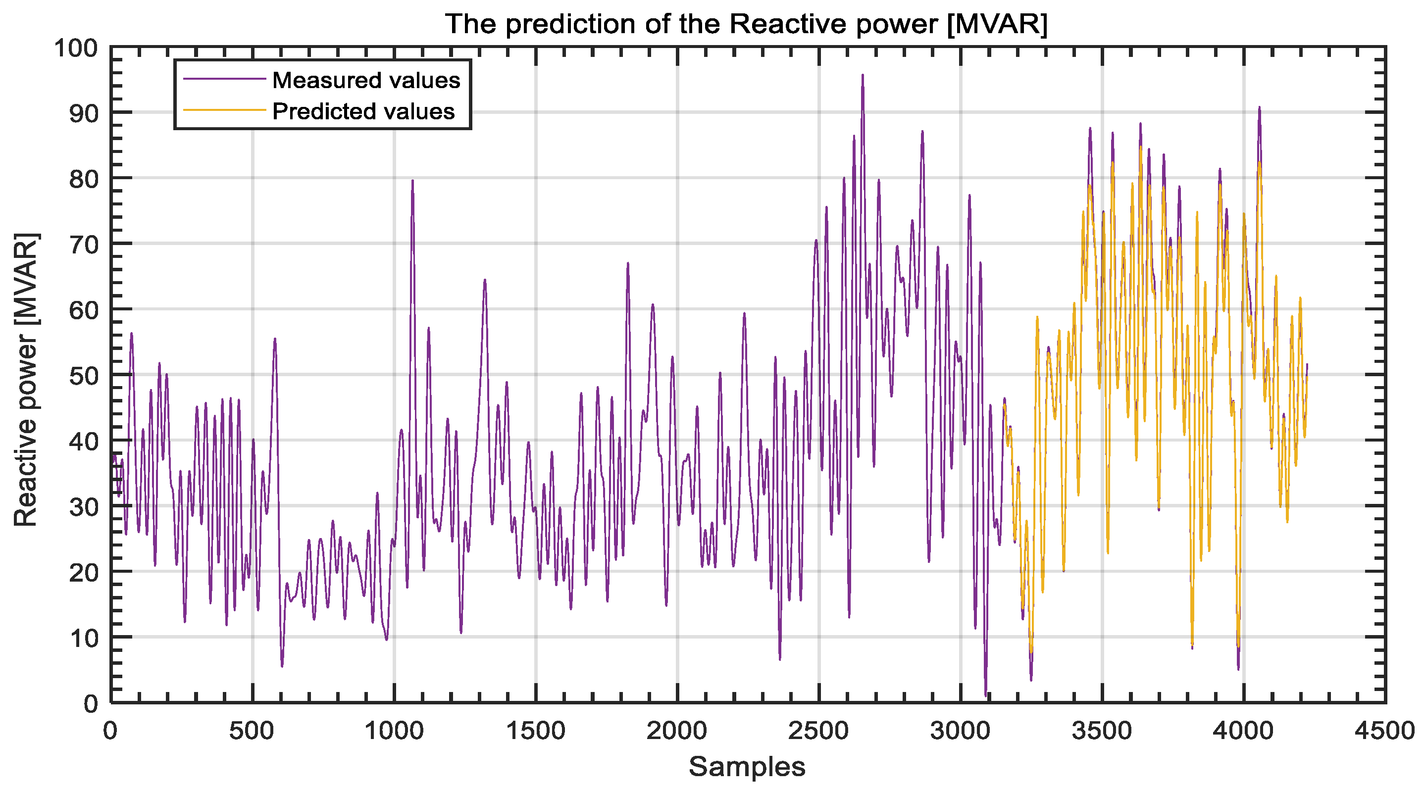
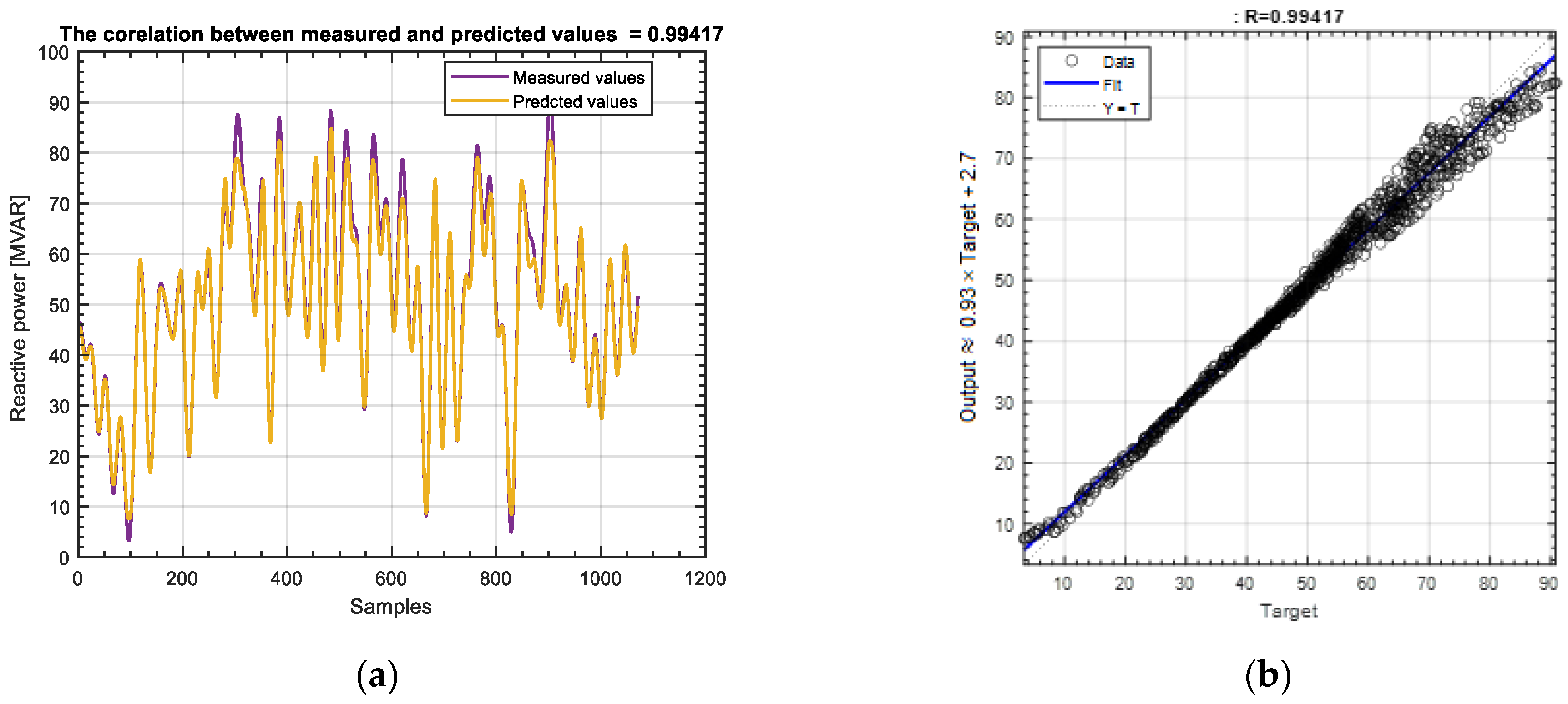
3.1.9. The Reactive Power (Q)

Reactive power, measured in volt–amperes reactive (VAR), is the power stored and released by the reactive elements and is as follows:

$$Q=V·I·sin\left(\phi \right),$$

(9)

3.1.10. The Distorted Power (D)

Distorted power occurs due to harmonics in the system and can be calculated using the relation (10), where $I_{rms}^2$ represents the sum of the squares of the harmonic currents as follows:

$$D=V·I_h=, V·\sqrt{I_{rms}^2-I_1^2}$$

(10)

where $I_{rms}$ is the effective value of the total current, and $I_1$ is the fundamental component of the current.

The relationship between apparent, active, reactive, and distorted powers is given by the following Equation (11):

$$S^2=P^2+Q^2+D^2$$

(11)

As a result, a detailed analysis using FFT (Fast Fourier Transform) was conducted [22]. The Fast Fourier Transform (FFT) was chosen for its computational efficiency and reliability in isolating harmonic components in the power quality data. The Fast Fourier Transform (FFT) is a very effective algorithm for computing the Discrete Fourier Transform (DFT) and its inverse [22]. The DFT is a mathematical approach that converts a sequence of values (a signal in the time domain) into frequency components. The FFTs are commonly utilized in signal processing. The FFT was applied to current and voltage signals. Thus, Figure 4a,b displayed the values of current and voltage harmonics in the melting phase obtained through FFT. The graphics are displayed using a logarithmic scale.

Figure 4a clearly shows a significant peak in the voltage harmonics at the lower frequency range, particularly around the fundamental frequency. This result is expected since this frequency corresponds to the main operating frequency of the EAF. Figure 4 illustrates that there are both even and odd harmonics in the voltage and current spectra during the melting phase. The presence of even-order harmonics in the melting phase indicates the electric arc behaves as if it were randomly varying in length.

Higher harmonics can be observed, with their magnitude decreasing as the frequency increases. There appears to be a clear difference in the harmonic content between the three phases, indicating that there may be variations in the power quality of each phase. The differences between phases occur due to the load being asymmetrical or the operation being unbalanced during the melting process. Higher harmonics are more noticeable in the voltage spectrum, with significant magnitudes even at higher frequencies.

The spectra for the three phases show a similar pattern, although with varying magnitudes. The current harmonics have a peak at the fundamental frequency, as seen in Figure 4b. There are noticeably higher harmonics in the current spectrum, indicating the presence of non-linearities caused by the arc and the load during the melting process.

The system’s non-linearity results from the dynamic behavior of the arc during the melting process, causing rapid fluctuations in the current. The variations in phases come from the complex and unpredictable behavior of the arcs, which can differ for each electrode.

During the refining stage, the voltage and current harmonic content show a more reduced spectrum and lower magnitudes for the higher harmonics, as depicted in Figure 5a,b. There is a noticeable peak at the fundamental frequency, while the higher harmonics are not as prominent. During the refining stage, the arc activity tends to be less intense than during the melting stage, resulting in a decrease in harmonic distortion in the voltage and current. Operating in a stable and controlled manner is indicated by the lower magnitude of higher harmonics. The spread between the three phases is smaller in comparison to the melting stage, suggesting a more uniformly distributed load. The refining process is not as intense as melting, resulting in fewer abrupt fluctuations in current and reduced harmonic distortion. In the refining phase, as shown in Figure 5, the voltage spectrum includes the fundamental component as well as the 5th and 7th order harmonics; however, the others are considerably reduced. Harmonics of orders 5 and 7 are observed with greater amplitudes in the current spectrum, as compared to harmonics of orders 11 and 13, but with smaller amplitudes.

It is important to note that, while harmonics of any order can be observed during the melting phase, both the voltage and current harmonics in the stable burning phase of the arc are characterized by the absence of harmonics, which has an order that is a multiple of three. This result is due to the connections of the windings of the furnace transformer. Harmonics of multiples of three of the electric current generate zero-sequence systems (homopolar); therefore, their propagation is blocked in Y connections without a neutral conductor.

Figure 6, Figure 7, Figure 8 and Figure 9 display the harmonic spectra for voltage and current on three phases (phase 1, phase 2, phase 3) throughout the melting and refining stages of the electric arc furnace (EAF) process. The spectra are presented using stem plots, which provide a clear visualization of the amplitude of harmonics at different frequencies.

The spectra for all three phases (a, b, c) show a prominent peak at the fundamental frequency for both voltage (Figure 6) and current (Figure 7). Multiple harmonics at multiples of the fundamental frequency are noticeable. Phase 1 displays the highest amplitude harmonics, followed by phases 2 and 3. The higher harmonic content is a result of the non-linear behavior and significant distortion in the voltage waveform, likely caused by the highly dynamic and irregular arc during the melting process. The presence of substantial harmonic content beyond the fundamental frequency indicates significant distortion. The variations in harmonic amplitudes between phases indicate phase imbalance and non-uniform load distribution.

The spectra for all three phases (a, b, c) from Figure 8 and Figure 9 again show an obvious fundamental frequency component for both voltage and current. The harmonic content beyond the fundamental frequency is significantly reduced when compared to the melting stage. The decreased and consistent harmonic amplitudes indicate enhanced arc stability and decreased non-linearity in comparison to the melting stage. The consistent harmonic amplitudes across phases indicate a better load balance and reduced phase imbalance.

During the melting stage, there is a noticeable increase in the harmonic content of both voltage and current spectra. This suggests the presence of non-linear behavior and distortion caused by the dynamic nature of the arc. The refining stage demonstrates a decrease in harmonic content, indicating a more stable and controlled operation with improved power quality.

During the melting stage, there is a clear phase imbalance, with notable differences in harmonic amplitudes between phases.

During the refining stage, there is an obvious increase in the consistency of harmonic amplitudes across phases, suggesting a more balanced load and reduced phase imbalance.

Having a high harmonic content and phase imbalance can result in subpar power quality, heightened losses, and the risk of damaging equipment.

The refined harmonics and balanced operation indicate enhanced power quality and increased efficiency.

The apparent power of the complete steel batch is illustrated in Figure 10. The apparent power is zero during certain intervals, which is a result of the interruption of the electric furnace power supply for the execution of specific technological operations (such as the addition of elements to achieve the desired composition and the measurement of the batch’s temperature and composition). The apparent power is lower during the initial period, which corresponds to the melting phase. This outcome is due to the decrease in voltage supplied by the furnace transformer, which is on a lower voltage step, and the increased position of the electrodes to ensure protection against breakage, which results in a lower current. The amplitude of the apparent power is approximately constant and higher than in the melting phase during the refining phase. This result is due to the furnace transformer operating on a higher voltage step and the operator typically sustaining a constant arc current. The apparent power increases once more by transitioning to a higher voltage step of the furnace transformer during the reduction (deoxidation) phase and the end of the refining phase.

The active, reactive, and distorted powers are presented in Figure 11, Figure 12 and Figure 13 for the same steel series. Figure 14 shows THD over the same time interval. In total, 4800 samples were represented graphically. Analyzing these graphs, it can be observed that, in all of them, there are intervals during which certain technological operations were carried out, with the electrodes being raised.

In MVA, apparent power is the overall power entering the system, including active and reactive power. The graph indicates large process fluctuations, with peaks up to 150 MVA. Significant variations show that EAF processes are dynamic, with power requirements changing substantially during melting and refining.

Active power (MW) is the actual power used to do the process (“melting steel”). Active power spikes correspond to the apparent power graph, showing most of it is used. Active power is more stable but still fluctuates due to steelmaking’s high-intensity energy bursts.

Reactive power (measured in MVAR) is likewise high, affecting the entire process. Figure 12 depicts the variation in reactive power, which shows that it is lower in the melting phase and higher in the oxidation phase.

Distorted power (in MVAD) mostly indicates power losses caused by harmonics. This graph shows consistent levels of distorted power with periodic big spikes, indicating when harmonic distortions can be quite strong. These distortions can also cause inefficiencies in steel production.

The THD is a percentage measure of harmonic distortions relative to the fundamental frequency. The graph demonstrates that THD normally remains below 1.8%; however, there are periodic increases, particularly during power surges. High THD levels may indicate poor power quality.

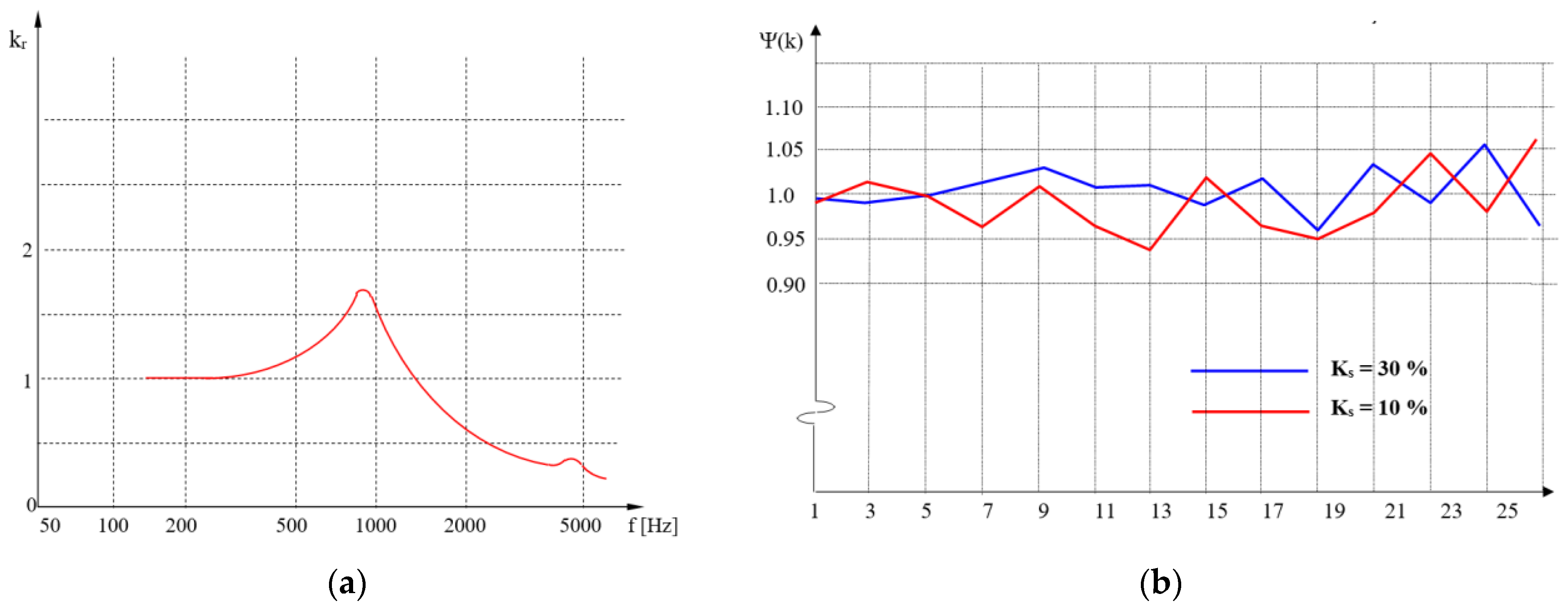
3.2. The Error Measure Analysis

The acquired data are processed in real time due to the integrated controller, which is equipped with FPGA and real-time technologies. The hardware–software system’s performance provides accuracy and reliability for application development, requiring high-speed response to meet measurement precision requirements.

Based on the information provided, it is clear that the measurement errors at 50 Hz are mainly caused by the errors introduced by the already indicated current and voltage transformers. Since harmonics have an important influence in determining the three-phase powers under deforming conditions, the additional errors caused by measurement transformers due to the frequency dependency of the relative transformation ratio were investigated.

The relative transformation ratio is defined as the ratio between the actual and nominal transformation ratios. Figure 15a depicts how the relative transformation ratio evolves with frequency for the voltage transformers in use. Figure 15b depicts the same fluctuation, but as a function of harmonic order, for current transformers having load levels of 30% and 10%, respectively. Knowing this variation, the required adjustments can be carried out with a software program, implemented in Matlab 2022a; these results are presented in

Table 1. The frequency dependence of three-phase powers.

No. of Sample	The Powers without Corrections				The Powers with Corrections				εS (%)	εP (%)	εQ (%)	εD (%)
	S	P	Q	D	S	P	Q	D
20	41.46	27.11	29.94	9.34	41.08	26.82	29.64	9.47	0.92	1.07	1.04	−1.43
200	44.21	19.46	38.00	11.46	43.79	19.26	37.62	11.47	0.95	1.04	1.03	−0.07
860	38.59	36.95	8.17	7.56	38.22	36.57	8.09	7.61	0.95	1.02	0.94	−0.60
1600	49.49	37.03	24.76	21.56	49.01	36.66	24.52	21.36	0.99	1.01	1.00	0.92
2320	68.58	49.70	45.63	12.33	67.93	49.20	45.16	12.40	0.97	1.02	1.02	−0.56
2800	64.94	49.90	39.70	12.29	64.32	49.40	39.29	12.33	0.97	1.01	1.03	−0.29
3200	72.25	48.63	52.43	10.29	71.55	48.14	51.90	10.42	0.97	1.01	1.03	−1.27
3600	55.80	51.35	18.63	11.40	55.27	50.83	18.43	11.46	0.96	1.02	1.06	−0.51
4000	63.92	50.09	37.33	13.56	63.32	49.58	36.95	13.61	0.96	1.02	1.03	−0.37
4480	33.04	29.94	12.19	6.81	32.72	29.64	12.07	6.80	0.96	1.00	0.99	0.11

. The frequency influence errors were computed at 20 points, among the all charge. It can be proven that the frequency influence errors are approximately 1%.

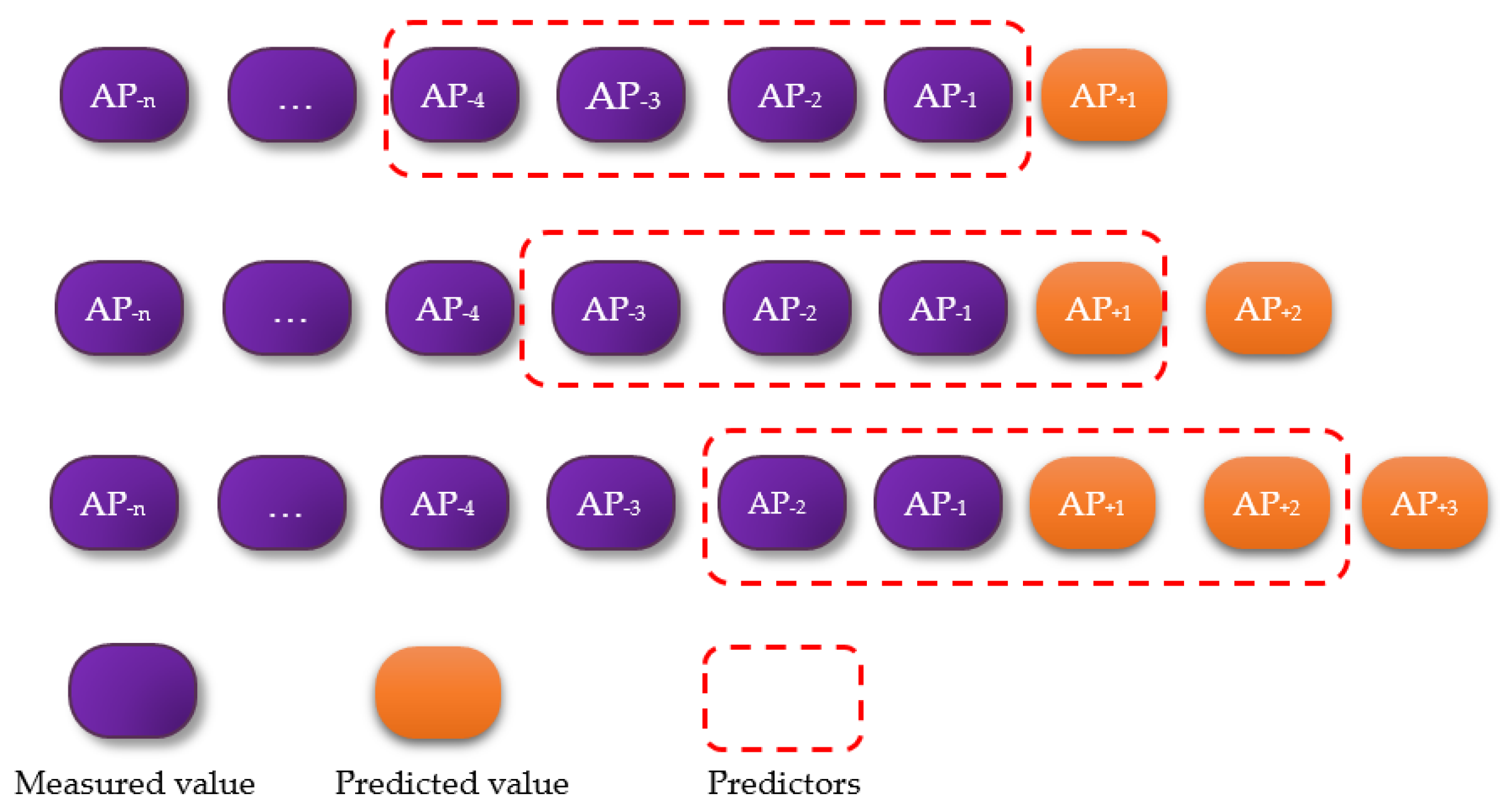
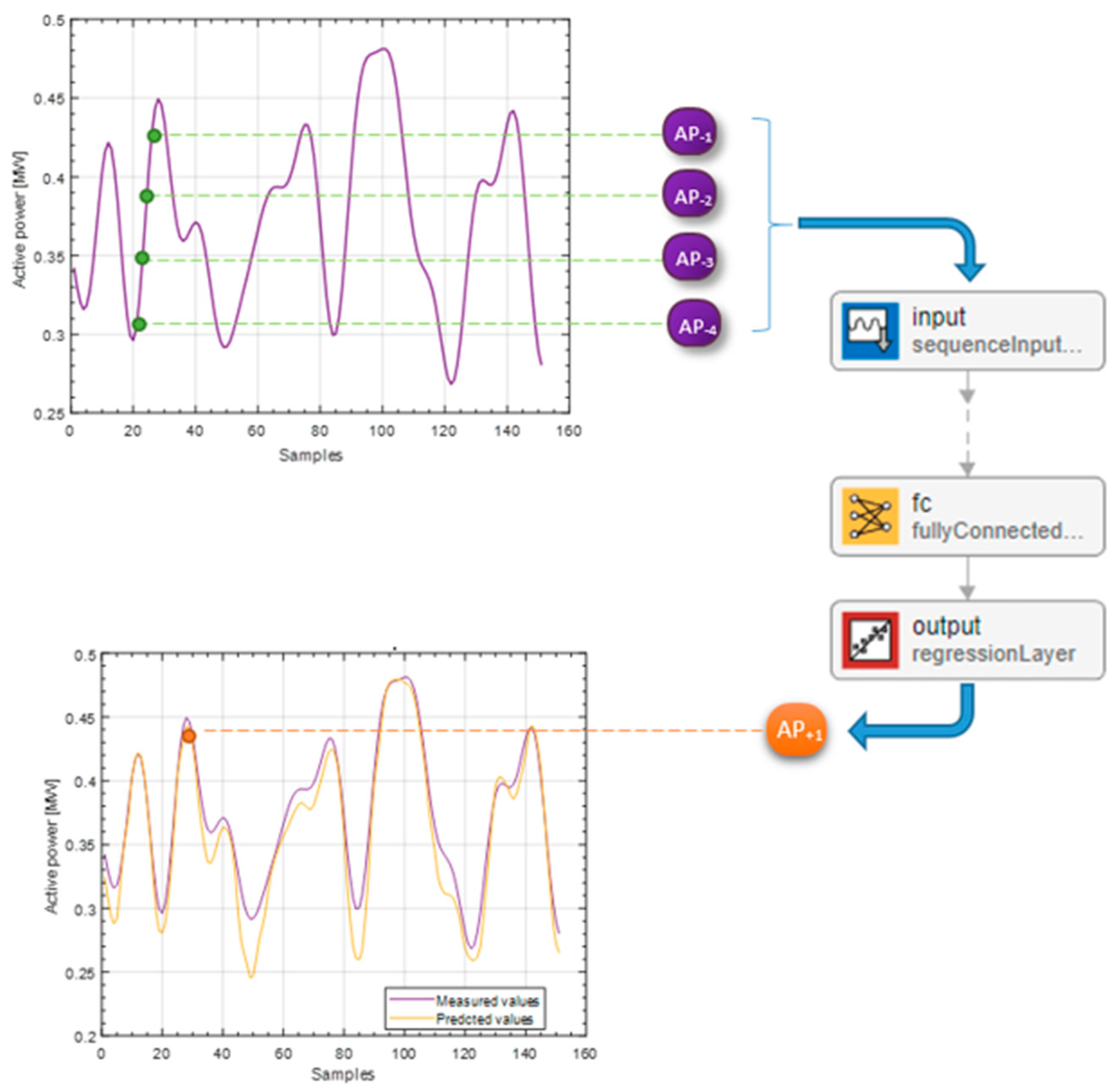
3.3. Hybrid Deep Neural Network in Analyzing Power Quality of EAF

In an electrical system with harmonic distortions, all four types of power—apparent (S), active (P), reactive (Q), and distorted (D)—are essential for analyzing and managing power quality. The active power is important because it indicates the actual power needed to melt the load in the oven container. The THD is also of great importance, as it is one of the main indicators for analyzing power quality.

Active power forecasting is essential for controlling energy efficiency, predicting consumption, and lowering operating costs [23]. Active power forecasting is used in an EAF to improve operational cycles and reduce electricity expenditures. Because of this, it was decided to create a forecasting model for active power.

However, the developed model can also be employed for apparent, reactive, distorted power or THD.

Deep neural networks (DNNs) have shown very good results in time-series prediction for active power forecasting in high-power loads like an EAF. This process involves estimating future active power consumption using historical data, which is important for efficient energy utilization and a stable system [24,25,26]. A Deep Neural Network (DNN) is a type of artificial neural network composed from multiple layers of neurons (also known as nodes) that interconnect the input and output layers. These networks are identified as “deep” because they contain more than one hidden layer, which enables them to reproduce complex, hierarchical data structures [24].

Deep neural networks (DNNs) use several relevant layers to process and manipulate data for time-series forecasting. The input layer receives raw data first. This layer usually represents historical data points for time-series data. Recurrent layers can handle sequential data and keep temporal dependencies, making them appropriate for time-series forecasting. Recurrent Layers include LSTM and GRU [24,25]. Also utilized in time-series prediction are convolutional layers. Conventional convolutional layers are used in image processing but can also forecast time series [23,27]. These layers use temporal convolution. They are used to identify time-series patterns like trends and seasonal components [28]. The dense layers are conventional neural network layers with every neuron coupled to the previous and next layer. These layers are utilized at network ends. Previous layers’ high-level features are combined to generate the final forecast. Time-series forecasting may generate one value (e.g., the next time step) or a sequence of values. Regularization with dropout layer prevents overfitting [23,29]. Activation functions give networks non-linearity to learn complex interactions. The final prediction is from the output layer. The forecasting task determines the activation function.

Data from both the melting stage and the refining stage were utilized to train the DNN. This training developed the model to be used for predictive purposes during the refining phase. In general, data from the refining stage are more suitable for training a CNN for prediction purposes for the following reasons: Signals that are more stable and less chaotic are more conducive to enhanced feature learning. The model’s capacity to learn and generalize patterns is facilitated by its consistent power characteristics.

Nevertheless, if the objective is to create a model that can effectively manage the chaotic and transient conditions of the melting stage, it may be necessary to integrate data from both phases. This method guarantees that the model has been exposed to the complete spectrum of operational conditions.

The structure of the DNN used for the power prediction is depicted in Figure 16.

The “Input” Layer takes sequences of active power values as input data. The “Fold” Layer prepares the input sequence for convolution. Local patterns from input data are extracted by the “ConvLayer” using 2D convolution on folded sequences. The “BatchNormLayer” normalizes previous layer activations at each batch, reducing training time and overfitting. The Exponential Linear Unit (ELU) activation function produces model non-linearity. The “PoolingLayer” reduces feature map spatial dimensions. Flattening the input into a vector is the “Flattenlayer” function. The “GRULayer” layer captures data temporal dependencies. The GRUs efficiently learn long-term dependencies. The “LSTMLayer” processes sequencing data. Learning long-term dependencies allows LSTMs to be useful for the vanishing gradient problem. Dropout Layers have the role of a regularization layer and prevents overfitting by randomly setting a fraction of input units to zero at each training update. The “LSTMbil”, the bidirectional LSTM Layer, processes input sequences forward and backward, capturing previous and future states. The “Fully” Layer maps the previous layers’ high-level features to the output space. The final layer provides the network’s prediction.

In this study, a single-step prediction and a multi-step prediction were performed. Figure 17 illustrates both types of prediction. In the case of a single-step prediction, the network is trained to predict the next step from the time-series data (one step ahead). The multi-step prediction is a recursive multi-step prediction. This kind of prediction was performed during testing, but also it was performed for unknown data (so called prediction beyond the horizon). In case of a recursive multi-step prediction for testing after making an initial prediction, the predicted value is fed back into the model as an input for predicting the next step. This process is repeated for each subsequent prediction, updating the sequence with the predicted values. The beyond horizon prediction extends the recursive multi-step prediction approach for a larger number of steps, defined by the horizon variable.

The multiple inputs of the Deep Neural Network are sequences of active power values, AP_-n, AP_-(n−1) … (AP₋₁), as can be seen in Figure 17 and Figure 18. The model utilizes time-series data to represent active power and other power quality indicators, such as reactive power, distorted power, or THD. To predict future values of the same indicators, the hybrid deep neural network analyzes these inputs using layers such as the CNN, LSTM, and GRU.

The predicted values of power quality indicators, including active power, reactive power, distorted power, and total harmonic distortion (THD), are the output of the neural network. The outputs can be either a single-step prediction, AP + 1, or a multi-step prediction.

3.4. Performance Indicators

For analyzing the results, the following main evaluation metric were used: RMSE, R-squared, MSE, MAE, sMAPE [23,24,30].

Equations (12)–(16) present these performance indicators. In these equations, it was noted that AP was the Active Power for which the modeling and prediction were performed. Also, n is the number of data, ${AP}_i$ is the measured value of Active Power at step i, and $\widehat{{AP}_i}$ is the estimated value of Active Power at the step i.

3.4.1. Mean Absolute Percentage Error (MAPE)

Forecasting model accuracy is measured by Mean Absolute Percentage Error (MAPE), shown in Equation (12). The accuracy as a percentage is the average absolute difference between the measured and forecasted values relative to measured values.

$$MAPE={\displaystyle \frac{1}{n}}\sum _{i=1}^n\left|{\displaystyle \frac{{AP}_i-\widehat{A{P}_i}}{{AP}_i}}\right|$$

(12)

3.4.2. Symmetric Mean Absolute Percentage Error (SMAPE)

The sMAPE is calculated using Equation (13) and is a useful indicator for evaluating forecasting models, especially when the data include values of different scales.

$$SMAPE={\displaystyle \frac{1}{n}}\sum _{i=1}^n{\displaystyle \frac{2\left|{AP}_i-\widehat{{AP}_i}\right|}{\left|{AP}_i\right|+\left|\widehat{{AP}_i}\right|}}$$

(13)

3.4.3. Root Mean Square Error (RMSE)

The RMSE is a common prediction model accuracy indicator. It is the square root of the average of the squared differences between the predicted and measured values.

$$RMSE\left({AP}_i,\widehat{{AP}_i} \right)=\sqrt{{\displaystyle \frac{1}{n}}{\left({AP}_i-\widehat{{AP}_i}\right)}^2}$$

(14)

3.4.4. Mean Absolute Error (MAE)

The MAE is a parameter also used to measure the accuracy of a predictive model. It represents the average of the absolute differences between the predicted values and the measured values.

$$MAE\left({AP}_i,\widehat{A{P}_i} \right)={\displaystyle \frac{1}{n}}\sum _{i=1}^n\left|{AP}_i-\widehat{{AP}_i}\right|$$

(15)

3.4.5. R² Coefficient

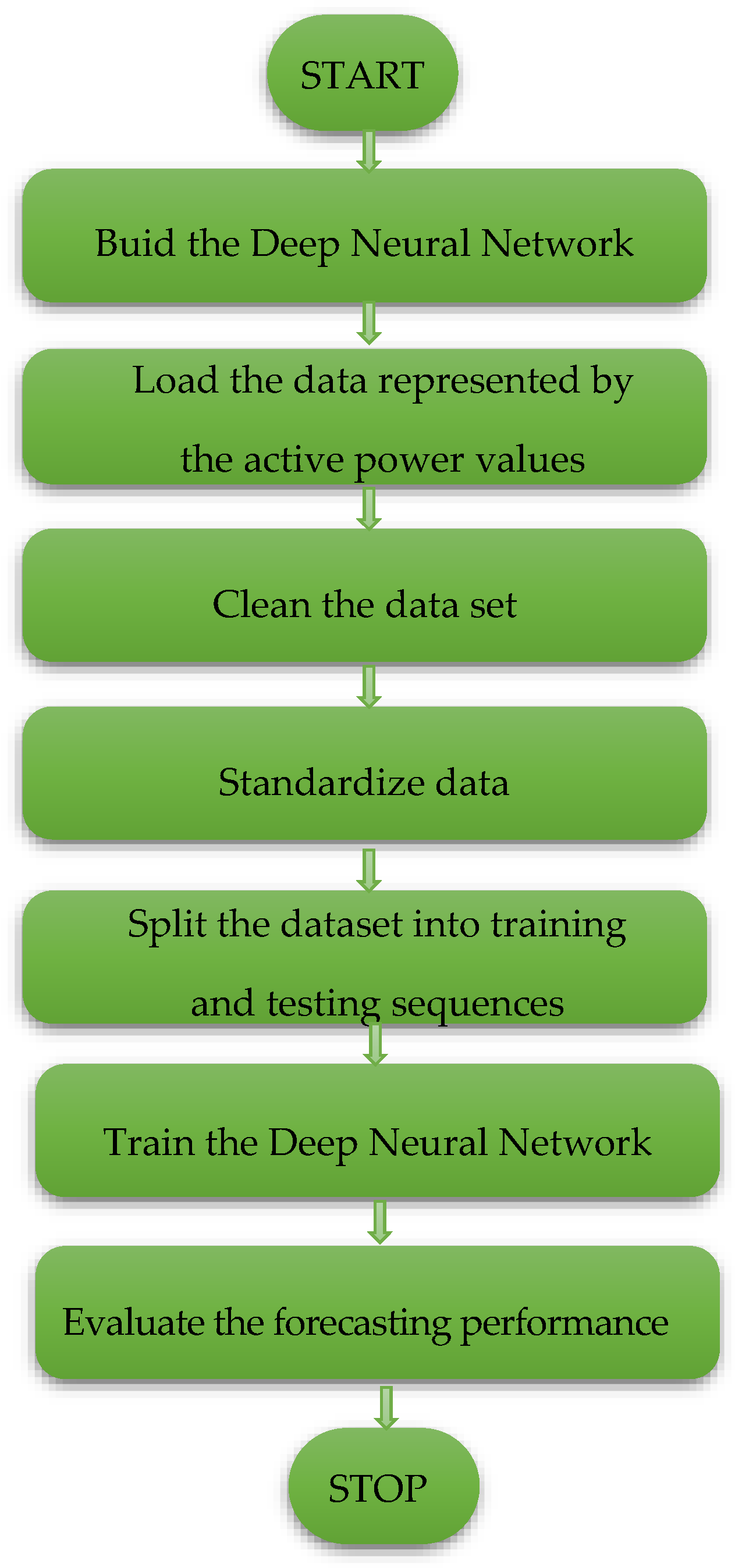
In the context of time-series forecasting, the R² coefficient (coefficient of determination) is used to evaluate how good is a forecasting model, showing how well the predicted values match the actual values over time.

$$R^2=1-{\displaystyle \frac{\sum _{i=1}^n{\left(A{P}_i-\widehat{{AP}_i}\right)}^2}{\sum _{i=1}^n{\left({AP}_i-\overline{A{P}_i}\right)}^2}}$$

(16)

while it is a useful metric, it should be utilized with other performance metrics (such RMSE, MAE, or sMAPE) to get an accurate assessment of model performance, especially in the presence of time-varying structures.

4. Results

Prior to training, data cleaning was performed because the measured data that were used for training the DNN contained temporal gaps. As a result, the steps that are utilized in forecasting are summarized in Figure 19. The hyper-parameters used for training the DDN are as follows:

• The ratio used for splitting training and testing data is as follows: 0.6 to 0.85.
• The number of precedents samples is as follows: between 200 and 500.
• The steps for multi-step prediction and horizon are as follows: between 500 and 1000.

Figure 20 is a representation of the dataset that was used after it was cleaned.

Figure 21 displays the training results, with 65% of the dataset being used for training and 35% being used for testing. It can be observed that the training is of very good quality. A coefficient sMAPE of 0.0052 was obtained for this model, which is a very good value. This means that the predicted values are very close to the measured ones, indicating that the model performed well in forecasting active power. Figure 21 shows the correlation between measured values and predicted values. The correlation coefficient of 0.99543 shows that the predicted values fit measured data well. The plot from Figure 22a indicates that the predicted curve (blue) line almost completely overlaps the measured (red) curve, that indicate a very good correlation. This result shows that the model captures active power series dynamics and is correctly anticipating the general trend and fluctuations and peaks.

Figure 22b shows the correlation between measured and predicted values. The data points are closely grouped around the blue linear fit line, indicating that the model predictions are accurate across target values. The linear fit line equation indicates Output ≈ 0.99 × Target + 0.42, which is close to the ideal Y = T. There is a small systematic bias where predictions are 1% below the target, although it is minimal, indicating small prediction errors. The minor offset in the fit line (with an intercept of approximately 0.42) suggests a small bias in the predictions, but the high correlation makes this bias likely insignificant.

Figure 23 shows a time-series graph comparing measured data (in red) to single-step prediction (blue) and “one step and update the data” (green) forecasts. The blue line shows model predictions during testing. Recursive forecasting, shown in green, forecasts one step ahead, then uses this prediction for predicting the next step. This method is used when is needed to make predictions one step at a time, updating the sequence with each new predicted value. The green line varies more from observed data than the blue “Forecast Testing”. While the recursive technique can extend predictions further into the future, each step generates additional error. Recursive multi-step forecasting frequently accumulates small errors, resulting in larger differences. Despite the larger error, it can be observed that there is still a good correlation between the predicted values and the measured values from the test sequence. It is useful when it is needed to dynamically update the model with new predictions.

Figure 23 presents the prediction of multiple steps without updating the sequence with measured values after each prediction. Predictions are made for a fixed number of future steps (defined by the horizon) without updating the sequence with observed data after each prediction. In the “Beyond the Horizon” prediction, the model uses an initial sequence of observed data to forecast a certain number of steps into the future (the horizon). After the model begins forecasting, it no longer uses the current observed data and instead relies only on its own prior predictions to forecast the upcoming values. This process can lead to error accumulation because each forecast relies on the one before it, and any minor error can be increased as the model produces subsequent predictions. The measured data, shown in red in Figure 24, have been included in the graph to offer a visual reference point for comparing predicted and actual results. Viewing the observed data with the model predictions (marked in green) enables a rapid and intuitive assessment of prediction accuracy. By comparing the two curves, it is possible to evaluate whether the model was able to capture the main patterns and trends in the measured data, or if there are large variations that suggest limitations in the model’s capacity to generate accurate long-term predictions. The graph demonstrates the model’s effectiveness. The predictions (green curve) closely reflect the observed data (red curve), indicating that the model has strong generalizability and can accurately forecast future active power values.

Furthermore, the hybrid deep neural network was used to forecast not only active power, but also other power quality indicators. The results section mainly highlighted the prediction of active power to demonstrate the robustness of this method; however, the model can also extend its ability to forecast reactive power, distortion power, and total harmonic distortion (THD). Therefore, the hybrid deep neural network was used to forecast reactive power, with the results of this prediction illustrated in Figure 25, Figure 26, Figure 27 and Figure 28, similar to the approach used to predict active power. Figure 25 presents the full sequence of the values for the reactive power used to train the hybrid DNN. These values were obtained after cleaning the data.

It can be observed that, just like in the prediction of active power, in the case of reactive power, the model successfully captures its fluctuations. This result can be observed both in Figure 26 and Figure 27a. However, it can be observed that in some areas of the graph there are some overestimates or underestimates of the measured values.

The regression analysis from Figure 27b also indicates a very good correlation between the measured and predicted values of the reactive power. The equation of the best fit line is given as Output ≈ 0.93 × Target + 2.7, indicating a slight bias and scaling difference in the prediction, as the slope is close to 1. Overall, the training phase of the model has very good results for the reactive power.

Figure 28a presents a multi-step prediction with the trained model. Figure 28a shows the following curves: measured values (the test data), single-step predicted values as well as multi-step predicted values. The prediction seems reasonably accurate; the green line (one-step-ahead prediction with sequence updates) follows the measured values. Figure 28b represents the correlation between the measured and predicted values.

Similar to the case of active power, the graph presented in Figure 28a also illustrates the model’s effectiveness for reactive power. The predictions represented by the green curve align closely with the measured values from the purple curve, suggesting that the model demonstrates efficient generalizability and is good for accurately forecasting future reactive power values.

5. Discussion

In this research, we developed forecasts for reactive power, as well as for distorted power and total harmonic distortion (THD). Overall, the results are satisfactory with regard to the performance characteristics. It was decided not to include all these data because it would be more interesting to present the forecasting of active power to highlight the possibility of employing Deep Neural Networks in power quality analysis. To investigate the effectiveness of the modeling, a study was conducted that used different values for the parameters that characterize the prediction model.

Table 2. The prediction performances of the Active Power.

Number of Previous Samples	Ratio between Training and Testing	RMSE	sMAPE	MAE	R
300	0.6	3.314413	0.020381	2.640818	0.932784
	0.65	3.113631	0.019159	2.363491	0.933585
	0.7	2.772064	0.017979	2.249753	0.942575
	0.75	2.554321	0.017291	2.027032	0.954922
	0.8	2.703436	0.017741	2.144316	0.944628
	0.85	2.197355	0.014936	1.80319	0.96907
320	0.6	4.427475	0.026606	3.51508	0.905221
	0.65	3.215631	0.020395	2.519334	0.929615
	0.7	3.325819	0.021575	2.632571	0.929156
	0.75	3.446187	0.02241	2.784356	0.911974
	0.8	2.446932	0.016907	1.993812	0.956757
	0.85	2.075665	0.013437	1.568379	0.97342
340	0.6	3.63967	0.022252	2.872954	0.924098
	0.65	3.751916	0.024204	2.982398	0.906847
	0.7	3.643837	0.024214	2.936227	0.904302
	0.75	2.882581	0.019911	2.403643	0.937951
	0.8	2.856469	0.018973	2.289497	0.939664
	0.85	2.796537	0.018814	2.187657	0.946595
360	0.6	4.565411	0.026749	3.511043	0.886226
	0.65	4.003983	0.02621	3.219417	0.879203
	0.7	3.487623	0.022634	2.744349	0.906444
	0.75	3.294766	0.021581	2.638397	0.921039
	0.8	3.451286	0.023981	2.81407	0.912688
	0.85	2.496078	0.016638	2.030982	0.963686
380	0.6	4.361974	0.026913	3.450132	0.88018
	0.65	4.15275	0.026569	3.352146	0.890026
	0.7	4.017251	0.026412	3.229326	0.878045
	0.75	3.067461	0.020094	2.431549	0.931187
	0.8	3.756365	0.025836	3.055964	0.895678
	0.85	3.014232	0.019905	2.437175	0.940705
400	0.6	4.966194	0.030891	3.987687	0.856531
	0.65	4.139194	0.02705	3.318692	0.868059
	0.7	3.686925	0.023995	2.897578	0.892862
	0.75	3.810963	0.023953	2.93027	0.894915
	0.8	3.470194	0.023951	2.837146	0.913756
	0.85	2.800888	0.018161	2.234741	0.943493

presents an evaluation of the performance of the active power prediction using the metrics sMAPE, RMSE, MAE, and R for several different configurations of the model. The metrics generally indicate an improvement as the ratio between training and testing increases (from 0.6 to 0.85), no matter the number of previous samples. As the training ratio increases, the Correlation Coefficient (R) consistently grows, demonstrating that the model utilizes a larger quantity of data to learn from. This learning is evident at the higher training ratios (e.g., 0.85), where R values frequently exceed 0.94, demonstrating a robust predictive relationship. The error metrics sMAPE, RMSE, and MAE generally decrease as the ratio increases, which indicates that the predictions are more accurate and there is less error. The model’s performance in terms of sMAPE and RMSE is slightly decreased when the number of previous samples used is smaller (e.g., 300 or 320), especially at lower training ratios. This performance means that the model’s capacity to accurately capture the trends in the active power variation decreases when it used a smaller number of prior samples. Generally, performance improves as the number of preceding samples increases. For example, the sMAPE, RMSE, and MAE are among the lowest recorded, while the correlation (R) is high, with 400 samples and a 0.85 ratio. It indicates that the model can make better forecasts when it is given information with a more extensive historical context. Using 400 previous samples with a 0.85 training/testing ratio results in the most optimal overall performance in terms of minimal error (sMAPE, RMSE, MAE) and high correlation (R). Here, the model obtains an R of 0.943493, an RMSE of 0.018161, and an sMAPE of 2.80088.

This configuration means the model has the ability to make accurate predictions with a significant relationship to the observed data by combining an adequate amount of training data with an appropriate context (number of previous samples).

Table 3. The prediction performances of the Reactive Power, Distorted Power, and THD.

The Power Quality Indicator	Number of Previous Samples	Ratio between Training and Testing	RMSE	sMAPE	MAE	R
Reactive power	300	0.65	4.013783	0.056213	3.523698	0.896213
		0.7	4.026241	0.036312	3.429386	0.876654
	400	0.65	3.568147	0.030571	2.853147	0.916471
		0.7	3.643837	0.044214	3.295413	0.900214
Distorted power	300	0.65	3.985413	0.025468	2.985466	0.902145
		0.7	4.153654	0.065413	3.254687	0.894123
	400	0.65	2.292016	0.009181	1.576199	0.995645
		0.7	2.983621	0.016243	2.014785	0.985464
THD	300	0.65	0.061189	0.031250	0.048770	0.903144
		0.7	0.072546	0.046524	0.042158	0.956477
	400	0.65	0.069962	0.035276	0.053137	0.965752
		0.7	0.071456	0.021589	0.053177	0.972147

presents the results for the prediction for the other indicators of the power quality, reactive power, distorted power and Total Harmonic distortion.

Short-term variations, such as those produced by voltage sags and flicker, are common in EAF processes, especially during the melting process. In the hybrid DNN, Convolutional Neural Network (CNN) layers were used to capture localized patterns in the data being processed, while Long Short-Term Memory (LSTM) and Gated Recurrent Units (GRU) efficiently handled the time-series data’s sequential dependencies, capturing both short-term and long-term fluctuations.

These recurrent layers enabled the model to correct for rapid modifications in power quality indicators, resulting in precise predictions of sudden variations in current and voltage.

6. Conclusions and Future Work

The proposed hybrid deep neural network architecture, which combines LSTM, GRU, and CNN layers, demonstrates great accuracy in forecasting power quality indicators such as active power, reactive power, and total harmonic distortion. Conventional machine learning methods include linear regression, logistic regression, support vector machines, and classic neural networks. Both linear regression and classical neural networks were employed to model the power quality indicators for the dataset from the EAF. The findings of this research indicate that single-step prediction performs very well, but the multi-step prediction does not produce favorable results in case of traditional machine learning algorithms. Therefore, the results of prediction obtained from traditional machine learning methods were not included and the hybrid deep neural networks were implemented in our study.

The use of multi-step prediction allows effective forecasting even during the dynamic phases of the EAF cycle. The research shows that accurate prediction of power quality indicators can significantly mitigate the negative effects of EAFs on the electrical network including harmonic distortion, voltage sags, and flicker. Better forecasting allows the EAF process to be improved, which helps the electrical grid and energy efficiency.

The evaluation indicators of prediction quality, such as RMSE, MAE, and sMAPE, indicate that the developed model provides predictions with minimal errors, especially during the stable combustion phase, thus demonstrating the model’s reliability for industrial applications. The developed model can be integrated into real-time monitoring systems to assist in process control, improving both energy consumption and production efficiency. The multi-step prediction of active power is useful for optimizing the overall EAF operation. This process may help manage consumption of electricity and reduce costs. Understanding future power trends can help improve load balancing, minimizing spikes, and increasing power factor by properly managing harmonic filter installations and reactive power compensation.

Multi-step prediction of active and reactive power is useful for optimizing the overall EAF operation. This can help manage consumption of electricity and reduce costs. These benefits are obtained at almost no additional expense because the actual installations remain unchanged with the only changes comprising modifications to the soft control management.

Improved power quality in EAF operations has a significant economic benefit, since accurate forecasting can result in better energy usage, reduced costs, and increased life of the equipment through reducing power disturbances. In terms of energy, better control over reactive power and harmonic distortion results in reduced losses and increased overall efficiency, therefore directly influencing the energy efficiency of industrial processes.

From a social perspective, the reduction in power quality problems such flicker and harmonic distortion improves the stability of the grid, thus minimizing interruptions for other users connected along the same network.

References

1. Uz-Logoglu, E.; Salor, O.; Ermis, M. Online Characterization of Interharmonics and Harmonics of AC Electric Arc Furnaces by Multiple Synchronous Reference Frame Analysis. IEEE Trans. Ind. Appl. 2016, 52, 2673–2683. [Google Scholar] [CrossRef]
2. Nikolaev, A.A.; Anokhin, V.V.; Lozhkin, I.A. Estimation of accuracy of chosen SVC power for steel-making arc furnace. In Proceedings of the 2016 2nd International Conference on Industrial Engineering, Applications and Manufacturing (ICIEAM), Chelyabinsk, Russia, 19–20 May 2016; pp. 1–5. [Google Scholar] [CrossRef]
3. Brandão, D.A.D.L.; Parreiras, T.M.; Pires, I.A.; Braz de J. Cardoso, F. Electric Arc Furnace Reactive Compensation System Using Zero Harmonic Distortion Converter. IEEE Trans. Ind. Appl. 2022, 58, 6833–6841. [Google Scholar] [CrossRef]
4. Jebaraj, B.S.; Bennet, J.; Kannadasan, R.; Alsharif, M.H.; Kim, M.K.; Aly, A.A.; Ahmed, M.H. Power Quality Enhancement in Electric Arc Furnace Using Matrix Converter and Static VAR Compensator. Electronics 2021, 10, 1125. [Google Scholar] [CrossRef]
5. Ghiormez, L.; Panoiu, M.; Panoiu, C.; Rob, R. Electric Arc Model in PSCAD—EMTDC as embedded component and the dependency of the desired Active Power. In Proceedings of the 2016 IEEE 14th International Conference on Industrial Informatics (INDIN), Poitiers, France, 19–21 July 2016; pp. 351–356. [Google Scholar]
6. Balouji, E.; Salor, Ö.; McKelvey, T. Deep Learning Based Predictive Compensation of Flicker, Voltage Dips, Harmonics and Interharmonics in Electric Arc Furnaces. IEEE Trans. Ind. Appl. 2022, 58, 4214–4224. [Google Scholar] [CrossRef]
7. Nooshabadi AM, E.; Sadeghi, S.; Hashemi-Dezaki, H. Optimal Electric Arc Furnace Model’s Characteristics Using Genetic Algorithm and Particle Swarm Optimization and Comparison of Various Optimal Characteristics in DIgSILENT and EMTP-RV. Int. Trans. Electr. Energy Syst. 2022, 2022, 9952315. [Google Scholar] [CrossRef]
8. Babaei, Z.; Samet, H.; Jalil, M. Enhanced models with time-series coefficients used for electric arc furnace. IET Gener. Transm. Distrib. 2023, 17, 2301–2316. [Google Scholar] [CrossRef]
9. Babaei, Z.; Samet, H. Optimized time varying parameters of the power balance equation model for electric arc furnaces. IET Gener. Transm. Distrib. 2024, 18, 779–792. [Google Scholar] [CrossRef]
10. Marulanda-Durango, J.; Zuluaga-Ríos, C. A meta-heuristic optimization-based method for parameter estimation of an electric arc furnace model. Results Eng. 2023, 17, 100850. [Google Scholar] [CrossRef]
11. Marulanda-Durango, J.; Escobar-Mejía, A.; Alzate-Gómez, A.; Álvarez-López, M. A Support Vector machine-Based method for parameter estimation of an electric arc furnace model. Electr. Power Syst. Res. 2021, 196, 107228. [Google Scholar] [CrossRef]
12. Čerňan, M.; Müller, Z.; Tlustý, J.; Valouch, V. An improved SVC control for electric arc furnace voltage flicker mitigation. Int. J. Electr. Power Energy Syst. 2021, 129, 106831. [Google Scholar] [CrossRef]
13. Babaei, Z.; Samet, H.; Jalil, M. An innovative approach considering active power and harmonics for modeling the electric arc furnace along with analyzing time-varying coefficients based on ARMA models. Int. J. Electr. Power Energy Syst. 2023, 153, 109377. [Google Scholar] [CrossRef]
14. Laketic, N.; Radakovic, J.; Majtal, Z. Power factor correction of electric arc furnace using active and passive compensation. In Proceedings of the 2017 International Symposium on Power Electronics (Ee), Novi Sad, Serbia, 19–21 October 2017; pp. 1–6. [Google Scholar] [CrossRef]
15. Klimas, M.; Grabowski, D. Application of long short-term memory neural networks for electric arc furnace modeling. Appl. Soft Comput. 2023, 145, 110574. [Google Scholar] [CrossRef]
16. Balouji, E.; Salor, Ö.; McKelvey, T. Predictive Compensation of EAF Flicker, Voltage Dips Harmonics and Interharmonics Using Deep Learning. In Proceedings of the 2021 IEEE Industry Applications Society Annual Meeting (IAS), Vancouver, BC, Canada, 10–14 October 2021; pp. 1–10. [Google Scholar] [CrossRef]
17. Xu, H.; Shao, Z.; Chen, F. Data-Driven Compartmental Modeling Method for Harmonic Analysis—A Study of the Electric Arc Furnace. Energies 2019, 12, 4378. [Google Scholar] [CrossRef]
18. Severoglu, N.; Salor, O. Statistical Models of EAF Harmonics Developed for Harmonic Estimation Directly From Waveform Samples Using Deep Learning Framework. IEEE Trans. Ind. Appl. 2021, 57, 6730–6740. [Google Scholar] [CrossRef]
19. Panoiu, M.; Ghiormez, L.; Panoiu, C. Adaptive Neuro-Fuzzy System for Current Prediction in Electric Arc Furnaces. Adv. Intell. Syst. Comput. 2015, 1, 423–437. [Google Scholar] [CrossRef]
20. Panoiu, M.; Panoiu, C.; Sora, I.; Osaci, M. Simulation results on the reactive power compensation process on electric arc furnace using PSCAD-EMTDC. Int. J. Model. Identif. Control 2007, 2, 250. [Google Scholar] [CrossRef]
21. Panoiu, M.; Panoiu, C.; Sora, I.; Osaci, M. Using a model based on linearization of the current-voltage characteristic for electric arc simulation. In Proceedings of the 16th IASTED International Conference on Applied Simulation and Modelling, Palma de Mallorca, Spain, 29-31 August 2007; pp. 99–103. Available online: http://dl.acm.org/citation.cfm?id=1659062 (accessed on 1 February 2024).
22. Kalair, A.; Abas, N.; Kalair, A.; Saleem, Z.; Khan, N. Review of harmonic analysis, modeling and mitigation techniques. Renew. Sustain. Energy Rev. 2017, 78, 1152–1187. [Google Scholar] [CrossRef]
23. Kontogiannis, D.; Bargiotas, D.; Daskalopulu, A. Minutely Active Power Forecasting Models Using Neural Networks. Sustainability 2020, 12, 3177. [Google Scholar] [CrossRef]
24. Lee, C.; Jeong, D.; Jang, Y.; Bae, S.; Oh, J.; Lim, S. A Hybrid Deep Neural Network Model for Photovoltaic Generation Power Prediction. In Proceedings of the 2022 25th International Conference on Electrical Machines and Systems (ICEMS), Chiang Mai, Thailand, 29 November–2 December 2022. [Google Scholar] [CrossRef]
25. Succetti, F.; Rosato, A.; Panella, M. An adaptive embedding procedure for time series forecasting with deep neural networks. Neural Netw. 2023, 167, 715–729. [Google Scholar] [CrossRef] [PubMed]
26. Succetti, F.; Rosato, A.; Araneo, R.; Panella, M. Deep Neural Networks for Multivariate Prediction of Photovoltaic Power Time Series. IEEE Access 2020, 8, 211490–211505. [Google Scholar] [CrossRef]
27. Anu Shalini, T.; Sri Revathi, B. Power Generation Forecasting Using Deep Learning CNN-based BILSTM Technique for Renewable Energy Systems. J. Intell. Fuzzy Syst. 2022, 43, 8247–8262. [Google Scholar] [CrossRef]
28. Yazici, I.; Beyca, O.F.; Delen, D. Deep-learning-based short-term electricity load forecasting: A real case application. Eng. Appl. Artif. Intell. 2022, 109, 104645. [Google Scholar] [CrossRef]
29. Panoiu, M.; Panoiu, C.; Ivascanu, P. Power Factor Modelling and Prediction at the Hot Rolling Mills’ Power Supply Using Machine Learning Algorithms. Mathematics 2024, 12, 839. [Google Scholar] [CrossRef]
30. Iordan, A.-E. An Optimized LSTM Neural Network for Accurate Estimation of Software Development Effort. Mathematics 2024, 12, 200. [Google Scholar] [CrossRef]
Figure 1. The measurement scheme from the secondary of the furnace transformer.
Mathematics 12 03071 g001
Figure 2. The currents and voltages on the EAF’s power supply line during the melting phase: (a) Arc voltage in the melting stage; (b) Arc current in the melting stage.
Mathematics 12 03071 g002
Figure 3. The currents and voltages on the EAF’s power supply line during the refining phase: (a) Arc voltage in the refining stage; (b) Arc current in the refining stage.
Mathematics 12 03071 g003
Figure 4. The harmonic spectrum of the voltage and current during the melting stage: (a) the harmonic spectrum of voltage; (b) the harmonic spectrum of current.
Mathematics 12 03071 g004
Figure 5. The harmonic spectrum of the voltage and current during the refining stage: (a) the harmonic spectrum of voltage; (b) the harmonic spectrum of current.
Mathematics 12 03071 g005
Figure 6. The three phase voltage amplitudes for harmonics during the melting stage: (a) voltage harmonics for phase 1; (b) voltage harmonics for phase 2; (c) voltage harmonics for phase 3.
Mathematics 12 03071 g006
Figure 7. The three phase voltage amplitudes for harmonics during the refining stage: (a) voltage harmonics for phase 1; (b) voltage harmonics for phase 2; (c) voltage harmonics for phase 3.
Mathematics 12 03071 g007
Figure 8. The three phase current amplitudes for harmonics during the melting stage: (a) current harmonics for phase 1; (b) current harmonics for phase 2; (c) current harmonics for phase 3.
Mathematics 12 03071 g008
Figure 9. The three phase current amplitudes for harmonics during the refining stage: (a) current harmonics for phase 1; (b) current harmonics for phase 2; (c) current harmonics for phase 3.
Mathematics 12 03071 g009
Figure 10. The variation of the apparent power throughout the entire process.
Mathematics 12 03071 g010
Figure 11. The variation of the active power throughout the entire process.
Mathematics 12 03071 g011
Figure 12. The variation of the reactive power throughout the entire process.
Mathematics 12 03071 g012
Figure 13. The variation of the distorted power throughout the entire process.
Mathematics 12 03071 g013
Figure 14. The variation of the THD throughout the entire process.
Mathematics 12 03071 g014
Figure 15. The relative transformation ratio: (a) Relative transformation ratio for voltage transformers; (b) Relative transformation ratio for current transformers.
Mathematics 12 03071 g015
Figure 16. The hybrid CNN network architecture.
Mathematics 12 03071 g016
Figure 17. Recursive single-step and multi-step prediction.
Mathematics 12 03071 g017
Figure 18. Details about the single-step prediction.
Mathematics 12 03071 g018
Figure 19. The steps used for analyzing the power quality using deep neural network.
Mathematics 12 03071 g019
Figure 20. The full sequence of the measured values of active power used to train the hybrid deep neural network.
Mathematics 12 03071 g020
Figure 21. The result of training using the following parameters: learning rate 0.006, previous samples: 400, 65% data used for training and 35% data used for testing.
Mathematics 12 03071 g021
Figure 22. The measured and predicted values for the test sequence: (a) the curve variation for measured and predicted values; (b) scatter plot of predicted versus measured (target) values for the active power.
Mathematics 12 03071 g022
Figure 23. The measured and predicted values for the multi-step prediction: (a) the curve variation for measured and predicted values; (b) scatter plot of predicted versus measured (target) values for the active power.
Mathematics 12 03071 g023
Figure 24. Multi-step prediction for a value of “horizon” 820.
Mathematics 12 03071 g024
Figure 25. The full sequence of the measured values of the reactive power used to train the hybrid deep neural network.
Mathematics 12 03071 g025
Figure 26. The result of training using the following parameters: learning rate 0.006, previous samples: 400, 65% data used for training and 35% data used for testing. sMAPE = 0.0091.
Mathematics 12 03071 g026
Figure 27. The measured and predicted values for the test sequence: (a) the curve variation for measured and predicted values; (b) scatter plot of predicted versus measured (target) values for the reactive power.
Mathematics 12 03071 g027
Figure 28. The measured and predicted values for the multi-step prediction: (a) the curve variation for measured and predicted values; (b) scatter plot of predicted versus measured (target) values for the reactive power.
Mathematics 12 03071 g028