Abstract
The integration of photovoltaic (PV) systems into traditional power grids introduces significant challenges in maintaining system stability, particularly in multi-area power systems. This study proposes a novel approach to load frequency control (LFC) in a two-area power system, where one area is powered by a PV grid and the other by a thermal generator. To enhance system performance, a cascaded control strategy combining a fractional-order proportional–integral (FOPI) controller and a proportional–derivative with filter (PDN) controller, FOPI(1+PDN), is introduced. The controller parameters are optimized using the spider wasp optimizer (SWO). Extensive simulations are conducted to validate the effectiveness of the SWO-tuned FOPI(1+PDN) controller. The proposed method demonstrates superior performance in reducing frequency deviations and tie-line power fluctuations under various disturbances. The results are compared against other advanced optimization algorithms, each applied to the FOPI(1+PDN) controller. Additionally, this study benchmarks the SWO-tuned controller against recently reported control strategies that were optimized using different algorithms. The SWO-tuned FOPI(1+PDN) controller demonstrates superior performance in terms of faster response, reduced overshoot and undershoot, and better error minimization.
Keywords:
two-area power system; renewable energy control; spider wasp optimizer; cascaded fractional-order controller; load frequency control MSC:
68T20
1. Introduction
Photovoltaic (PV) power generation has become increasingly significant in modern power systems because of its renewable nature and the reduction in associated costs. The integration of PV systems into multi-area power networks, particularly in combination with traditional thermal generators, introduces complex dynamic interactions that must be effectively managed to ensure system stability [1]. A typical configuration studied is the two-area system, where one area incorporates a PV grid and the other a thermal generator. In such systems, the balance between power generation and consumption is crucial, especially given the variability in load demands and the intermittent nature of solar energy.
A major challenge in these systems is maintaining this balance while minimizing frequency deviations and tie-line power exchanges between the areas [2]. In this regard, load frequency control (LFC) is essential in multi-area power systems to maintain system frequency within specified limits and to ensure the scheduled power exchange between areas through the tie-line [3]. The importance of LFC is amplified in systems integrating renewable energy sources such as PV, where power generation is subject to fluctuations due to environmental conditions [4]. Therefore, effective LFC strategies are necessary to mitigate the impact of these fluctuations on system stability, which has driven significant research into advanced control methods and optimization techniques to enhance LFC performance in systems with renewable energy integration [5].
Various control strategies have been explored to manage LFC in two-area systems. In that sense, traditional controllers like proportional–integral (PI), proportional–integral–derivative (PID), and their fractional-order counterparts have been widely used [6,7]. PI controllers are known for their simplicity and ease of implementation but may lack the robustness required for complex, multi-area power systems. PID controllers, which include a derivative component, offer improved response times and stability. However, in systems with significant nonlinearity and time delays, the performance of conventional PI and PID controllers can be suboptimal [8]. Such a case highlights the need for more advanced and flexible control strategies capable of handling the dynamic and uncertain nature of PV-integrated multi-area power systems.
To address these challenges, fractional-order PI (FOPI) controllers have also been introduced. The FOPI controller, in particular, offers enhanced flexibility and robustness in LFC applications [9]. By incorporating fractional calculus into the control strategy, FOPI controllers provide an additional degree of freedom, allowing for more precise tuning of the system’s dynamic response. This makes them particularly well-suited for PV-integrated two-area systems, where the variability and uncertainty inherent in renewable energy sources demand a more sophisticated control approach [10]. Considering these facts, this study employs a novel controller by employing a cascaded controller that combines a FOPI controller with filtered proportional-derivative (PDN) structure. The proposed cascaded FOPI(1+PDN) controller eliminates steady-state error, provides additional flexibility in tuning the system’s dynamic response, helps anticipate future errors, and enhances the robustness against noise.
The effectiveness of any control strategy, including the FOPI controller, is heavily dependent on the optimal tuning of its parameters. Given the complexity of LFC in modern power systems, finding these optimal parameters of the controllers requires advanced optimization techniques [11]. Traditional methods may fall short because of the nonlinear and multi-modal nature of the problem, leading to the exploration of metaheuristic algorithms [12]. As part of the above challenge, several optimization algorithms have been employed to optimize the parameters of controllers, thereby improving their adaptability to changing system conditions. For example, the whale optimization algorithm (WOA) has been used to optimize LFC in PV-integrated systems, showing enhanced performance over traditional methods [13,14]. Similarly, the slime mold algorithm (SMA) [15,16] and the reptile search algorithm (RSA) [17] have been applied to optimize control parameters in complex power systems, demonstrating the potential to improve control performance in renewable energy scenarios significantly. Other notable examples include the use of the firefly algorithm (FA) [18], modified grey wolf optimization (MGWO) [19], hybrid shuffled frog-leaping and pattern search algorithm (hSFLA-PS) [20], black widow optimization (BWO) [21], RIME algorithm [22], artificial rabbit optimization (ARO) [23], sea horse optimizer (SHO) [24], and reinforcement learning-based approaches [25] to enhance LFC in similar contexts.
In terms of the optimizer, this study introduces the spider wasp optimizer (SWO) [26] as a novel approach in order to contribute to the ongoing effort in this field. The SWO is a novel metaheuristic algorithm inspired by the predatory behavior of spider wasps. It balances exploration and exploitation effectively, making it a promising tool for solving complex optimization problems such as controller parameter tuning [26]. The reason for employing the SWO in this study is due to the fact that none of the previously proposed optimizers have demonstrated the level of performance achieved by the SWO in handling the complexities of LFC in PV-integrated systems. In the context of LFC, the SWO has been employed to optimize the parameters of cascaded fractional-order controllers by employing the integral of time-weighted absolute error as the objective function in order to ensure faster and more stable system responses [25], resulting in improved system performance [27]. By optimizing the parameters of the cascaded FOPI(1+PDN) controller, the SWO enhances system stability and robustness in PV-integrated two-area systems. This approach addresses the limitations of conventional controllers and introduces a flexible solution for the dynamic challenges posed by renewable energy integration.
The performance analysis of cascaded fractional-order controllers, optimized using the SWO, demonstrates significant enhancements in the stability and robustness of PV-integrated two-area systems. By leveraging the strengths of the SWO, the proposed control strategy not only improves frequency regulation but also adapts more effectively to the dynamic and uncertain nature of renewable energy sources [28]. In this regard, the present work introduces the following novelties:
- The proposed approach effectively combines a state-of-the-art metaheuristic optimization algorithm with fractional-order control techniques, offering a novel solution to the challenges associated with renewable energy integration into traditional power systems.
- The application of the SWO for tuning the cascaded FOPI(1+PDN) controller in a PV-integrated two-area system represents a significant advancement in the field.
- This study emphasizes the effectiveness of the FOPI(1+PDN) controller in managing the intricacies of PV-integrated systems
- This study represents one of the earliest applications of the SWO in the domain of LFC, showcasing its potential for solving complex power system challenges.
2. Spider Wasp Optimizer
The spider wasp optimizer (SWO) is an advanced optimization algorithm inspired by the natural behaviors of spider wasps, particularly their hunting, nesting, and mating practices [26]. This algorithm is designed to address complex optimization problems by emulating the strategic actions of spider wasps in their natural environment [29].
2.1. Behavioral Simulation
The SWO algorithm simulates the following key behaviors of spider wasps:
- Searching Behavior: The female spider wasp searches for a spider, which will serve as a host for her larva. This behavior corresponds to the exploration phase in the algorithm, where the search space is explored for potential solutions.
- Pursuit and Escape Behavior: After locating a suitable spider, the wasp paralyzes it and drags it to a prepared nest. This behavior represents the exploitation phase, where the algorithm focuses on refining the search around promising solutions.
- Nesting Behavior: The paralyzed spider is dragged into a nest, where the wasp lays her egg. This behavior is analogous to finalizing a solution in the optimization process.
- Mating Behavior: The SWO algorithm incorporates a mating process that mimics the genetic recombination of solutions, enhancing diversity and enabling the exploration of new potential solutions.
2.2. Mathematical Formulation of Behavioral Simulation
The mathematical formulation of the SWO [29] begins with the generation of an initial population (), where each individual represents a potential solution in a D-dimensional space. The initial population is generated as follows:
The spider wasps’ initial population () is represented as a matrix, where each row corresponds to a wasp and each column to a dimension of the problem.
The position of each wasp in the search space is initialized using (3).
where and are the lower and upper bounds of the search space, respectively, and is a random vector of dimension , uniformly distributed between 0 and 1.
2.2.1. Searching Stage (Exploration)
During the exploration phase, the position of each wasp is updated to search for the optimal prey (solution) using
where denotes the current iteration, and are positions of randomly selected wasps, and is a velocity factor calculated as
where is a normally distributed random number and is a uniformly distributed random number between 0 and 1. If the wasp misses the optimal prey location, it recalculates its position using
where is the position of another randomly selected wasp, and is defined in (7).
with being a parameter calculated in (8).
where is a number randomly generated between 1 and −2. To find the most promising locations and effectively explore the search space, (4) and (6) operate together. The decision between using (4) or (6) is made randomly, determining the next position of the female wasp.
where and represent two random values within the interval [0, 1].
2.2.2. Pursuit and Escape Stage (Exploitation)
Once the prey is located, the wasp updates its position to close in on the prey, with the following (10).
where is a distance control parameter that decreases from 2 to 0 as the iterations progress, modeled by (11).
where is another random number between 0 and 1 and is the maximum number of iterations. To further enhance the search and ensure the wasps can escape local optima, the SWO algorithm introduces additional mechanisms in the pursuit and escape phase. Equation (12) represents how the distance between a wasp and its prey (the potential solution) increases as the wasp continues its search
where is a vector derived from a normal distribution, which influences the extent of the wasp’s movement. As the iteration progresses, the value of gradually increases the distance between the wasp and the prey, effectively switching the behavior from exploitation (intensifying the search near the prey) to exploration (broadening the search area). This transition is controlled by the parameter , defined in (13) as follows:
This equation ensures that as the algorithm approaches its final iterations, the search gradually transitions from intensive local exploration to broader global exploration. Equation (14) formalizes the decision-making process between two potential movement strategies, combining the influence of both exploitation and exploration.
Finally, the interchange between the different phases of the search is managed by (15)
where is another random value in [0, 1] and is from (13). This equation allows the algorithm to dynamically choose between continuing with the current strategy or switching to another, based on the progression of the iterations and the randomness introduced by .
2.2.3. Nesting Behavior (Finalization)
In the SWO, nesting behavior is crucial for refining and exploiting the best solutions identified during the search process. This stage simulates the actions of the female spider wasp when she drags the immobilized prey into her nest to prepare for laying eggs. The corresponding mathematical representation of this behavior is provided in (16).
where represents the best solution found so far, and is a random number that influences the direction and magnitude of the adjustment, ensuring that the new position is closer to the optimal solution. Following this, the wasp’s position can also be updated using another mechanism represented by (17).
where is a step size influenced by a Lévy flight distribution, and is a binary vector that helps avoid overlapping of nests at the same location by adjusting the positions based on the interactions between randomly selected wasps , , and . To prevent the establishment of multiple nests at the same location, (18) defines as
where and are two random numbers in the range [0, 1]. The selection of whether to apply (16) or (17) is determined randomly, as described in (19).
Finally, (20) achieves a trade-off between the different behaviors by deciding whether the algorithm should continue refining the current best solutions or explore new ones.
where represents the index of the population, is the population size, and is defined in (13) as a parameter that decreases over time, promoting more exploration in early stages and more exploitation in later stages. Through these mechanisms, the nesting behavior in SWO efficiently balances exploration and exploitation, allowing the algorithm to converge on high-quality solutions while still maintaining diversity to avoid premature convergence. The combination of random decisions and strategic updates ensures that the SWO can effectively navigate complex search spaces, making it robust for various optimization tasks.
2.2.4. Mating Behavior
In the SWO, mating behavior plays a significant role in generating new candidate solutions, which can be seen as the algorithm’s method of introducing diversity into the population. During this phase, new “offspring” solutions are created through a crossover process between pairs of “parent” solutions, represented by the male and female wasps. The mathematical formulation of the crossover process is given by (21).
where represents the position of the female wasp, represents the position of the male wasp, and is the crossover rate, which dictates the likelihood that the crossover will occur between the two wasps. To introduce variability in the offspring, the male wasp’s position is updated with an additional component that adds diversity to the population. This update is captured by the following equation:
where the vectors and represent step sizes that determine the magnitude of the position change, while and are directional vectors calculated as represented in (23) and (24), respectively.
The vectors and guide the movement based on the relative fitness of the solutions ,,, and . This process ensures that the new positions are influenced by better-performing solutions, thereby improving the overall quality of the population in subsequent generations. The use of these parameters in the mating behavior ensures diversity and adaptability in the search process, allowing the algorithm to explore the solution space effectively while avoiding local optima.
2.3. Population Reduction and Memory Saving
In the SWO, population reduction and memory-saving strategies are critical for enhancing the optimization process. After the mating and hunting behaviors, the algorithm focuses on reducing the population size to accelerate convergence toward the optimal solution. This is achieved by gradually decreasing the number of spider wasps in the population while ensuring that the remaining individuals still maintain sufficient diversity to avoid being trapped in local optima. The population reduction mechanism is mathematically described by the following equation:
where represents the current population size, is the minimum population size required to maintain diversity, and is a control parameter that governs the rate of reduction. ensures that there are always enough search agents to explore the solution space effectively, even as the population is reduced. As the population size decreases, memory-saving techniques are employed to store the best solutions found during the optimization process. This approach ensures that even as the number of active search agents diminishes, the algorithm retains a record of the most promising solutions, which can be used to guide future generations. The memory-saving process is crucial for optimizing high-dimensional and complex problems, where maintaining a balance between exploration and exploitation is essential for achieving the best results.
3. System Modeling
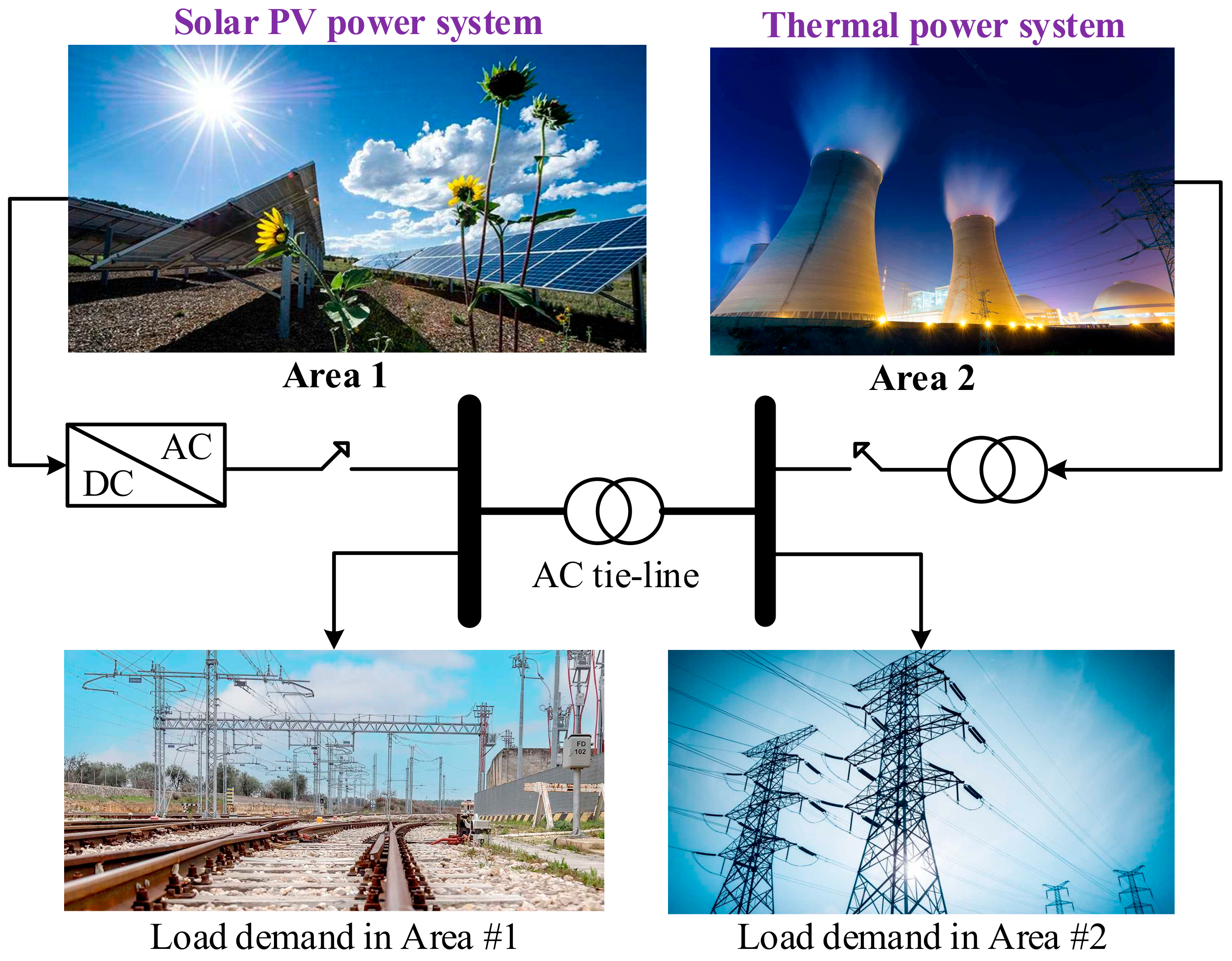
In a two-area power system composed of a PV grid and a thermal generator, the dynamic behavior of each area and their interaction through a tie-line are crucial for maintaining system stability and efficient power exchange. The thermal power system, consisting of components like the governor, reheater, turbine, and generator, can be mathematically modeled using transfer functions. The governor, which regulates steam flow in response to frequency deviations, is described by
where is the governor gain and is the time constant. The re-heater, which introduces a delay in the steam before it reaches the turbine, has the following transfer function:
where and represent the reheater gain and time constant, respectively. The steam turbine, converting thermal energy into mechanical power, is modeled as follows:
with being the turbine gain and the time constant. The generator, converting mechanical to electrical power, is represented by
where and are the generator gain and time constant. The PV system is characterized by its output power, dependent on solar irradiance and temperature, expressed as follows:
where is the efficiency, is the area of the PV panels, and is the solar irradiance. The inverter, converting DC to AC power, follows the dynamic
where and are the inverter gain and time constant. The overall behavior of the PV system can be encapsulated in the transfer function
The interaction between the two areas is managed through the tie-line, which facilitates power exchange. The tie-line power flow is modeled by
where is the synchronizing coefficient and , are the frequency deviations in the respective areas. Figure 1 visually represents the layout of the two-area system, highlighting the connection between the PV grid in Area 1 and the thermal power system in Area 2 via the AC tie-line.

Figure 1.
Layout of the two-area system employed in this study.
4. A Novel Control Strategy for Load Frequency Control
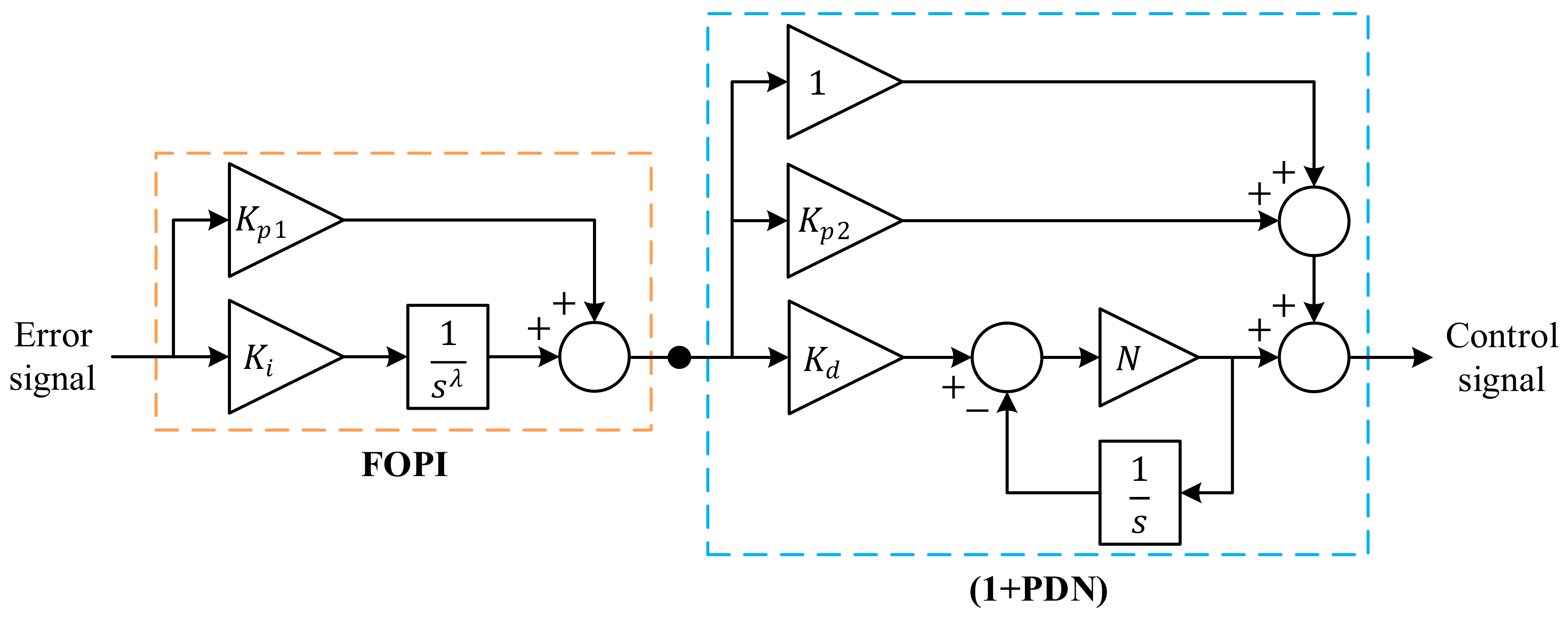
The proposed strategy employs a cascaded controller combining a FOPI controller with a PDN controller. The mathematical representation of the proposed controller is given by Equation (34).
where and are the proportional gains for the FOPI and PDN components, respectively. is the integrator gain in the FOPI controller, responsible for eliminating steady-state error, represents the fractional order of the integral component in the FOPI controller, providing additional flexibility in tuning the system’s dynamic response, is the derivative gain in the PDN controller, which helps in anticipating future errors based on the rate of change, and is the filter coefficient that moderates the high-frequency gain of the derivative term, enhancing the controller’s robustness against noise. The block diagram of the cascaded FOPI(1+PDN) controller is shown in Figure 2.
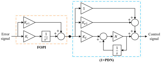
Figure 2.
Block diagram of the cascaded FOPI(1+PDN) controller.
The objective of this control strategy is to minimize the ITAE, a performance metric that emphasizes the importance of reducing error over time, thus ensuring faster and more stable system responses [24]. The objective function is mathematically expressed in Equation (35).
where s represents the total simulation time. and are the frequency deviations in Area 1 and Area 2, respectively. is the deviation in tie-line power between the two areas. This objective function is minimized under the scenario of Disturbance I, which involves a 10% step change in load in both areas of the power system. The goal is to achieve a controller configuration that minimizes these deviations and restores system stability as quickly as possible.
The block diagram illustrating the SWO-based tuning mechanism for the two-area power system with the FOPI(1+PDN) controller is presented in Figure 3. The two-area power system model shown in Figure 3 has been widely employed for testing the stability performance of various algorithms and controllers, as referenced in [1,13,18,19,20,21,22,25,27,30]. These references have used the same model parameters for system analysis based on a Simulink environment, which provides more flexible and comprehensive analyses compared with reduced transfer function models. The validity of this model covers typical operational conditions in multi-area power systems, including load variations and disturbances. The equations and transfer functions used in this model are based on standard system parameters, as outlined in the system modeling section (Section 3), ensuring it accurately represents real-world dynamic behavior under different disturbance scenarios.
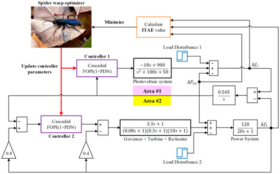
Figure 3.
Block diagram of the SWO-based tuning mechanism for a two-area power system with the FOPI(1+PDN) controller.
5. Simulation Results and Discussion
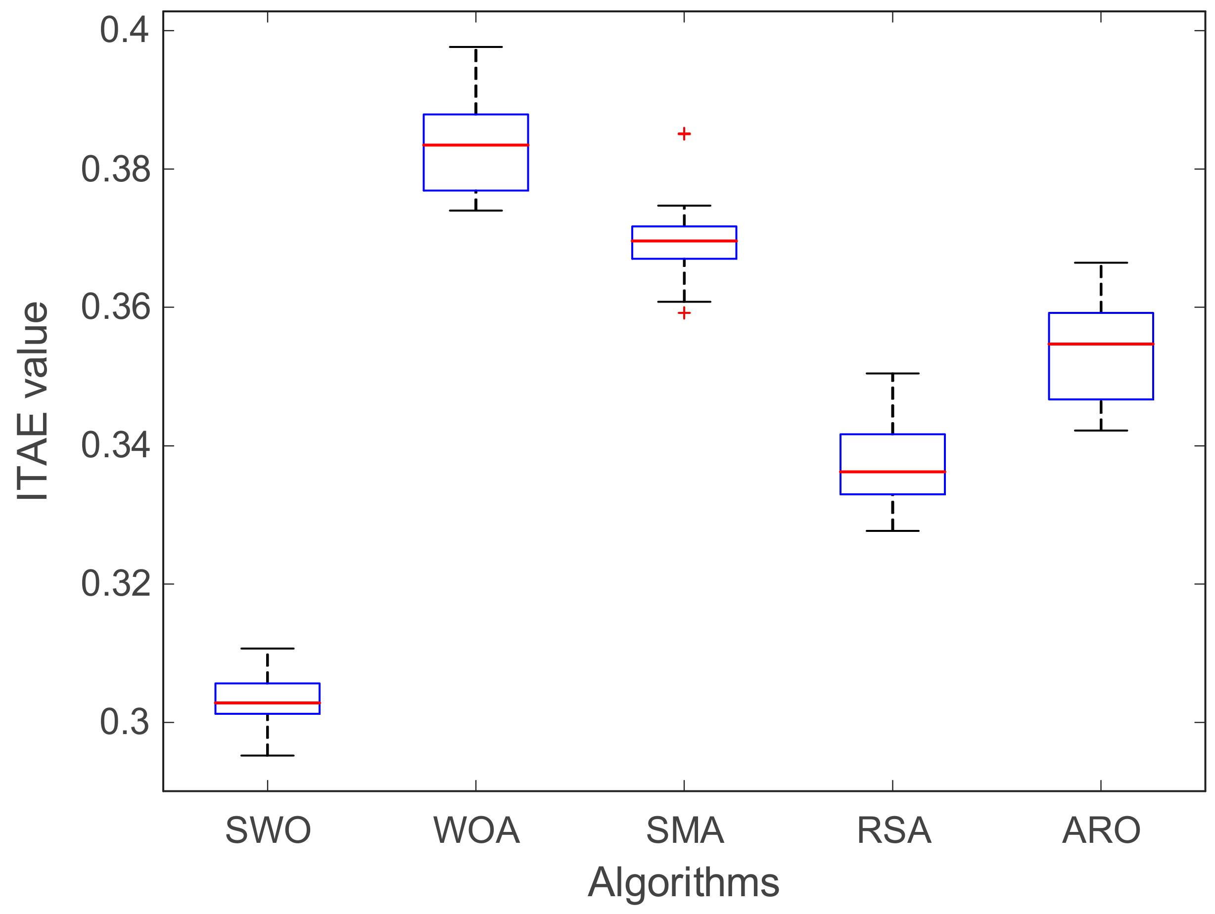
5.1. Statistical Success of the SWO
A thorough statistical analysis of the SWO in comparison with other well-known metaheuristic algorithms is presented, specifically the WOA, SMA, RSA, and ARO. The analysis is based on the results of 20 independent runs for each algorithm, focusing on their effectiveness in minimizing the ITAE within a two-area power system. Table 1 provides the parameter settings for each of the algorithms considered in this study, including the population size, number of function evaluations, and other specific control parameters that govern their search processes. It is important to note that the statistical performance of metaheuristic algorithms is primarily influenced by the number of function evaluations (NFE). Through detailed analysis, we determined that an NFE range of 3000–4000 provided the best balance between accuracy and computational efficiency for the SWO, WOA, SMA, RSA, and ARO algorithms, with 4000 being the optimal choice. This selection is supported by the literature [1,13,18,19,20,21,22,25,27,30], where NFE values typically range between 2500 and 5000.

Table 1.
Parameter values of the adopted algorithms.
To assess the performance and robustness of these algorithms, a boxplot analysis was conducted, as depicted in Figure 4. This figure illustrates the distribution of ITAE values achieved by each algorithm over 20 runs, providing insights into the variability and consistency in their performance. The boxplot reveals that the SWO exhibits a narrower range of ITAE values, indicating its robustness and reliability compared with the other algorithms.

Figure 4.
Boxplot analysis of the SWO, WOA, SMA, RSA, and ARO.
The outcome of a further analysis is shown in Table 2, which summarizes the statistical results obtained from the different algorithms. Key performance metrics, including the minimum, maximum, median, and average ITAE values, standard deviation (SD), and rank, are presented to offer a comprehensive comparison. The SWO consistently outperforms the other algorithms, as indicated by its superior rankings across most metrics.
Table 2.
Statistical results obtained across different algorithms.
To validate the superiority of the SWO over the other algorithms statistically, a non-parametric Wilcoxon signed-rank test was conducted. Table 3 presents the results of this test, including the p-values for comparisons between the SWO and the other algorithms (WOA, SMA, RSA, ARO). The table also indicates whether the SWO showed statistically significant superiority in each comparison.
Table 3.
Nonparametric statistical results obtained using the Wilcoxon test.
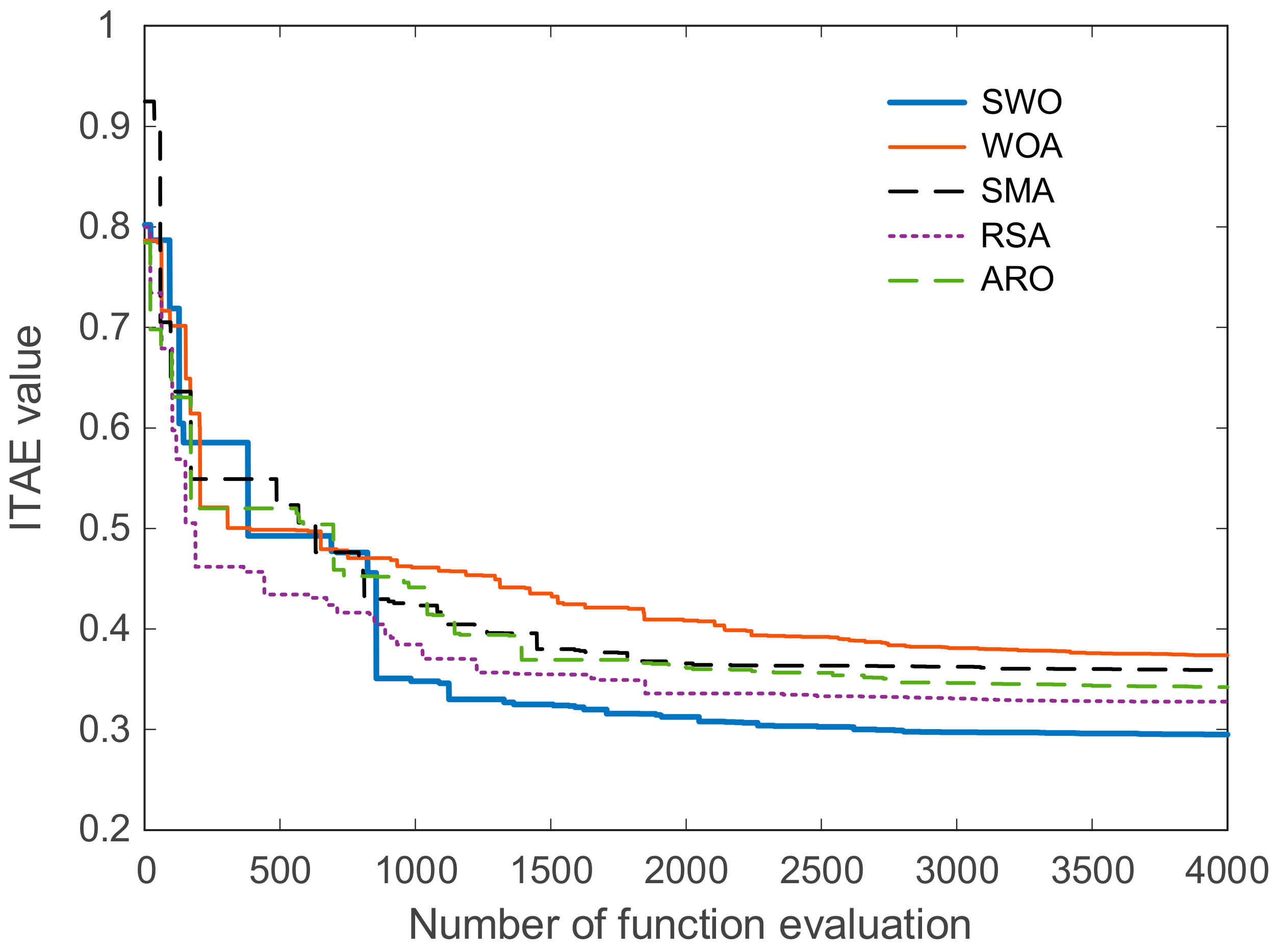
The convergence behavior of each algorithm was examined through a plot illustrating the change in ITAE values with respect to the number of function evaluations. Figure 5 shows how quickly each algorithm converges to an optimal solution, with the SWO demonstrating a more efficient convergence profile compared with the others. As illustrated in Figure 5, the ITAE objective function optimized by the SWO algorithm converges at 3000 NFEs and stabilizes beyond 4000 NFEs. Increasing NFE beyond 4000 does not improve the ITAE value but extends the computation time, making 4000 NFEs the ideal compromise between accuracy and computational cost.
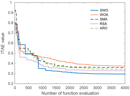
Figure 5.
Change in ITAE according to the number of function evaluations.
Table 4 provides a comparison of the controller parameters obtained through the optimization processes of each algorithm for the two areas of the power system. This table highlights the specific parameter settings achieved by each algorithm, offering a clear view of how each method optimizes the control strategy for load frequency control.
Table 4.
Obtained controller parameters via different algorithms.
The results from this statistical analysis confirm that the SWO is highly effective in optimizing control parameters for the two-area power system. The SWO not only consistently ranks highest in terms of statistical metrics but also demonstrates superior robustness and convergence efficiency compared with the other algorithms evaluated. These findings underscore the potential of the SWO as a powerful tool for optimizing advanced control strategies in complex power systems, particularly in contexts involving renewable energy integration. Furthermore, the parameters for the FOPI(1+PDN) controller were selected based on their standard operating ranges commonly used in power system stability studies. As shown in Table 4, the parameters are constrained within specific ranges to ensure stability and performance across different operating conditions. These ranges were chosen to allow the controller to handle typical disturbances in a two-area power system. However, it is important to note that these fixed parameter ranges might limit the controller’s performance under extreme conditions, such as sudden large-scale renewable energy input or severe system disturbances. Future research could explore more adaptive ranges or the use of real-time tuning to extend the controller’s effectiveness in broader operational scenarios.
5.2. Comparisons with Effective Algorithms
A detailed comparison of various metaheuristic algorithms in tuning the FOPI(1+PDN) controller for load frequency LFC in a two-area power system is offered in this section. The algorithms under comparison include the SWO, WOA, SMA, RSA, and ARO. The performance is assessed under two distinct disturbance scenarios, with a focus on frequency deviation in both areas and tie-line power fluctuations.
5.2.1. Disturbance I
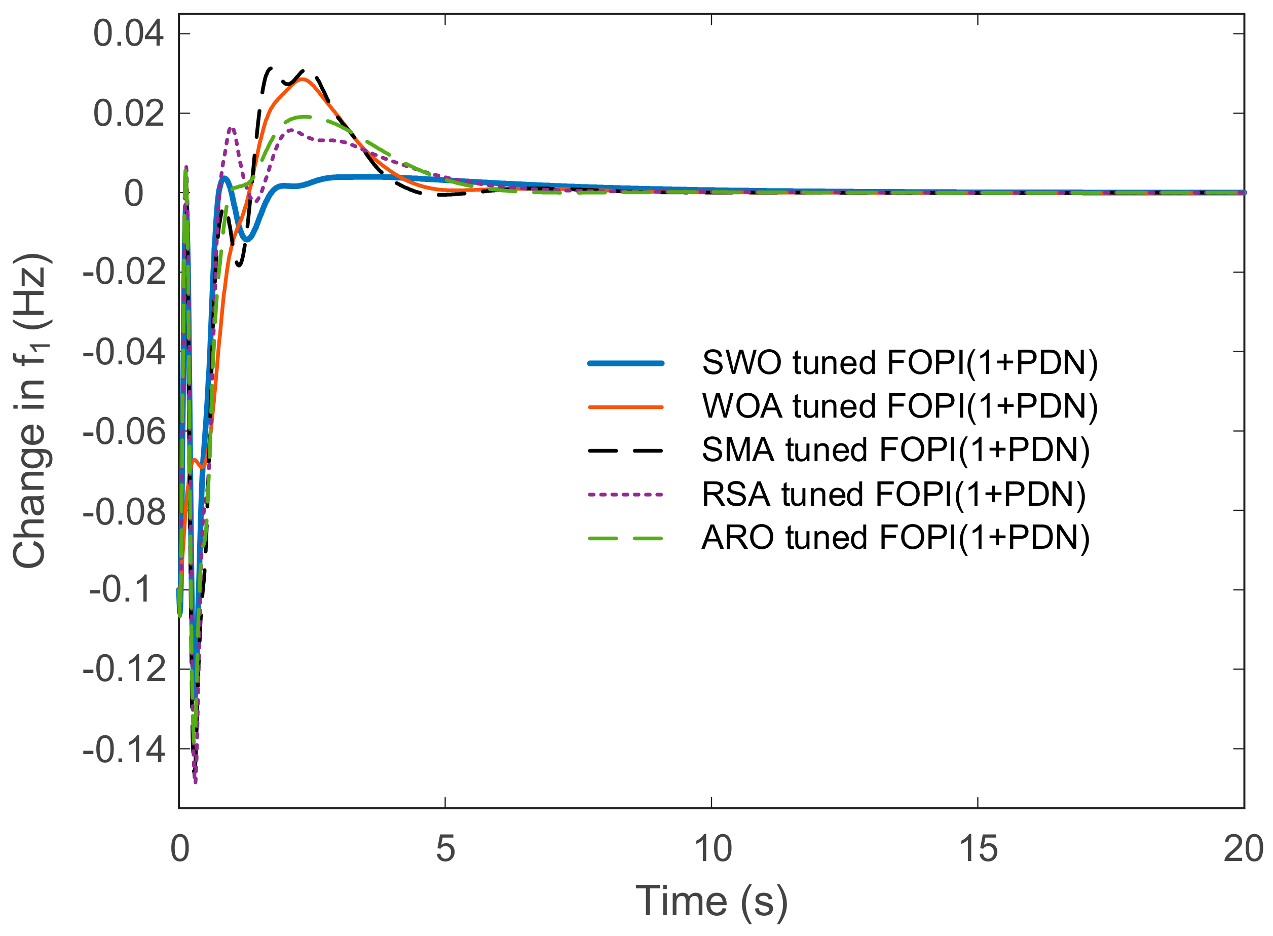
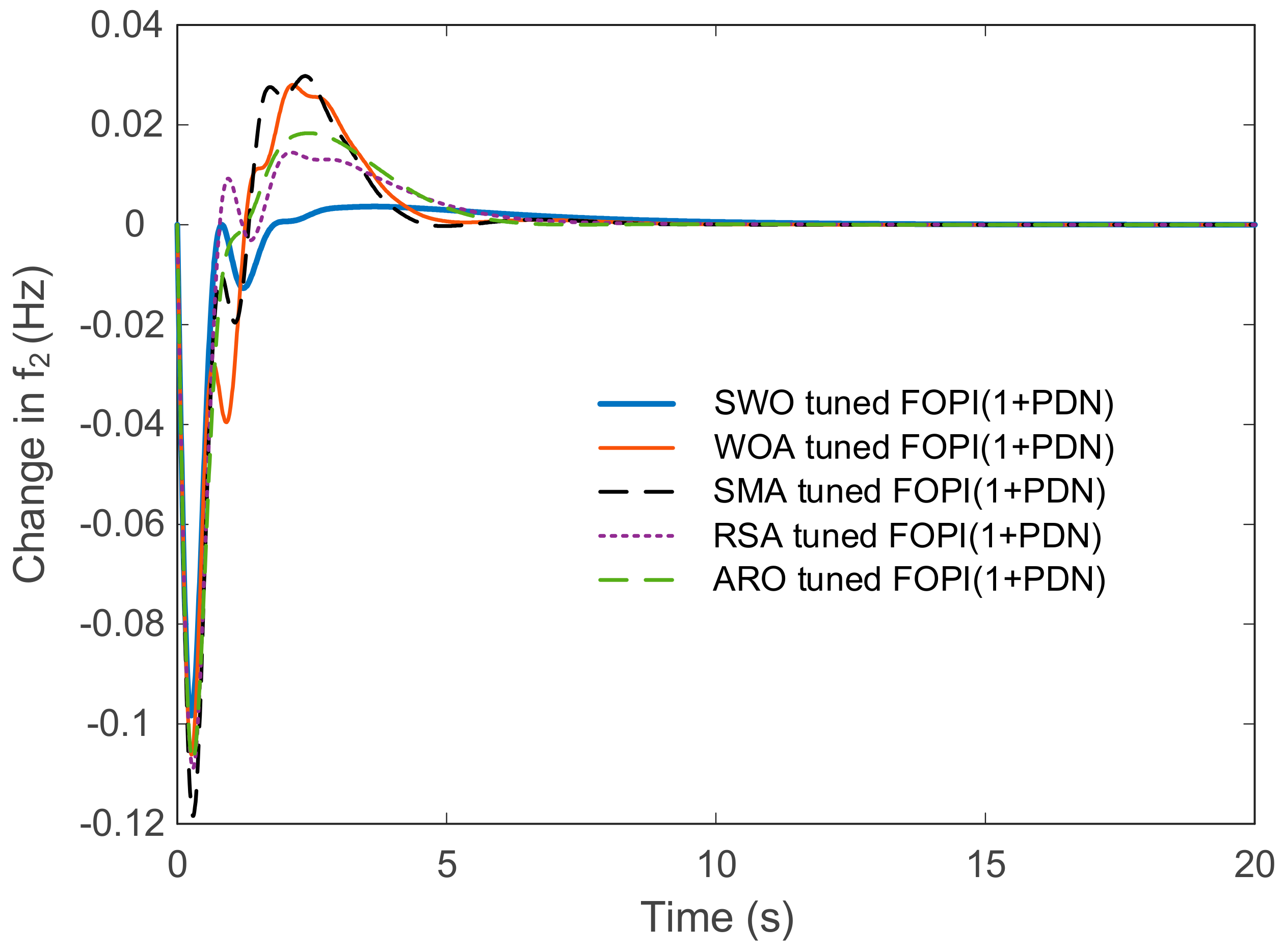
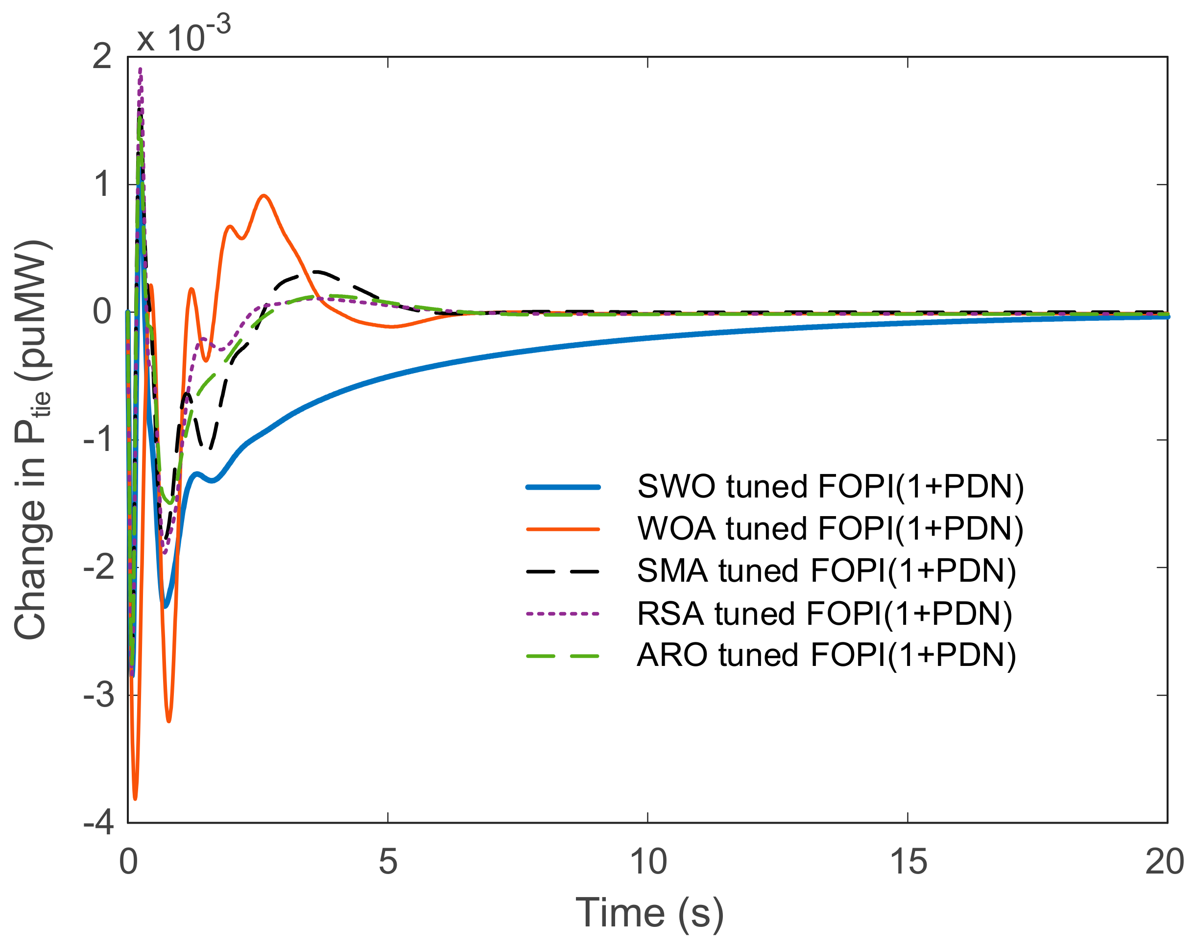
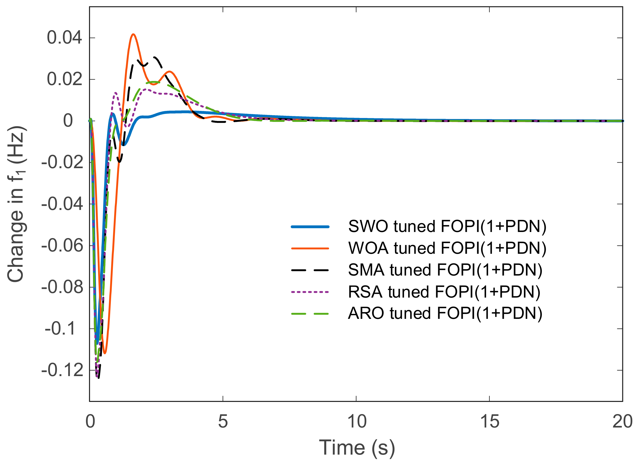
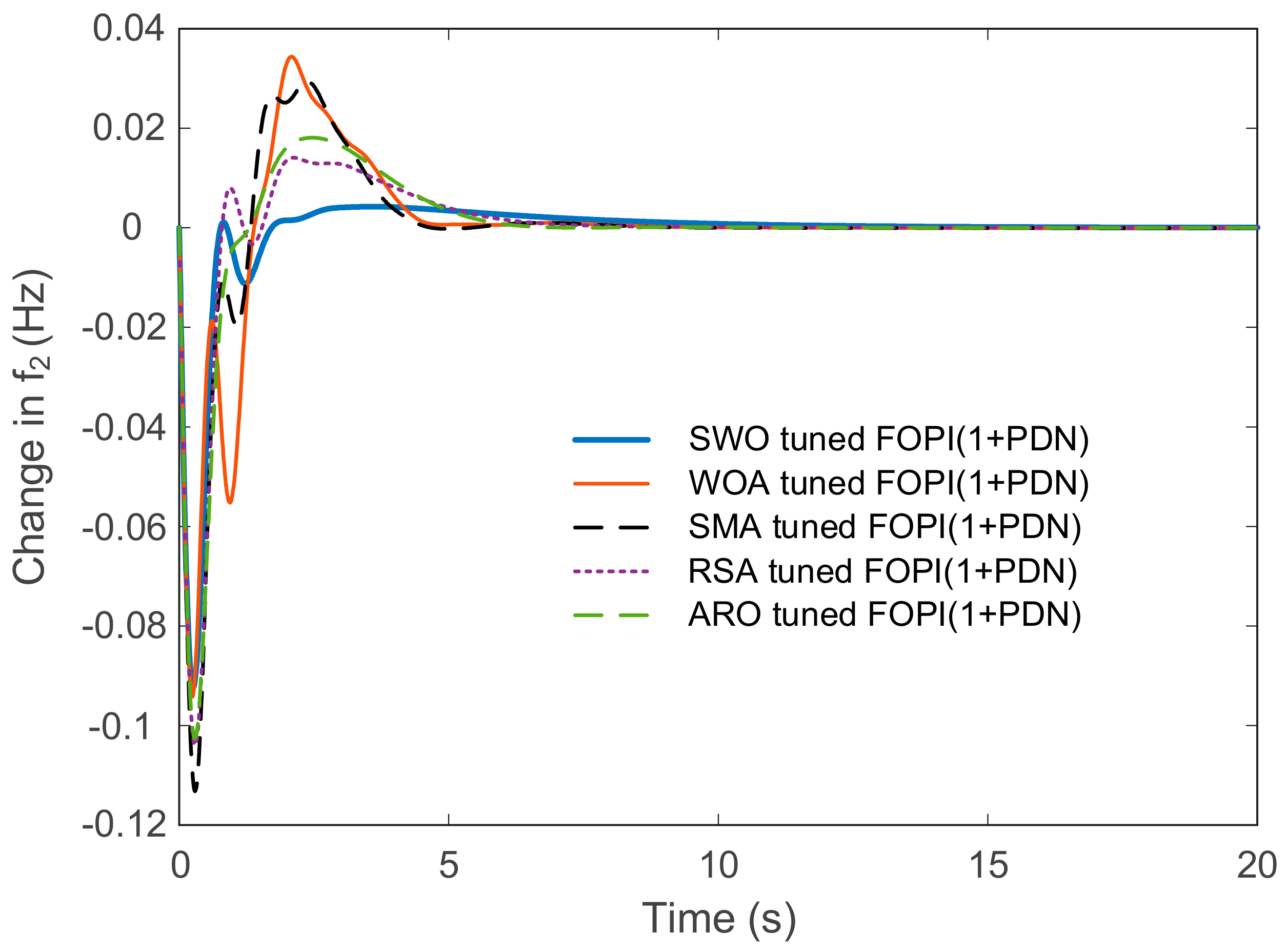
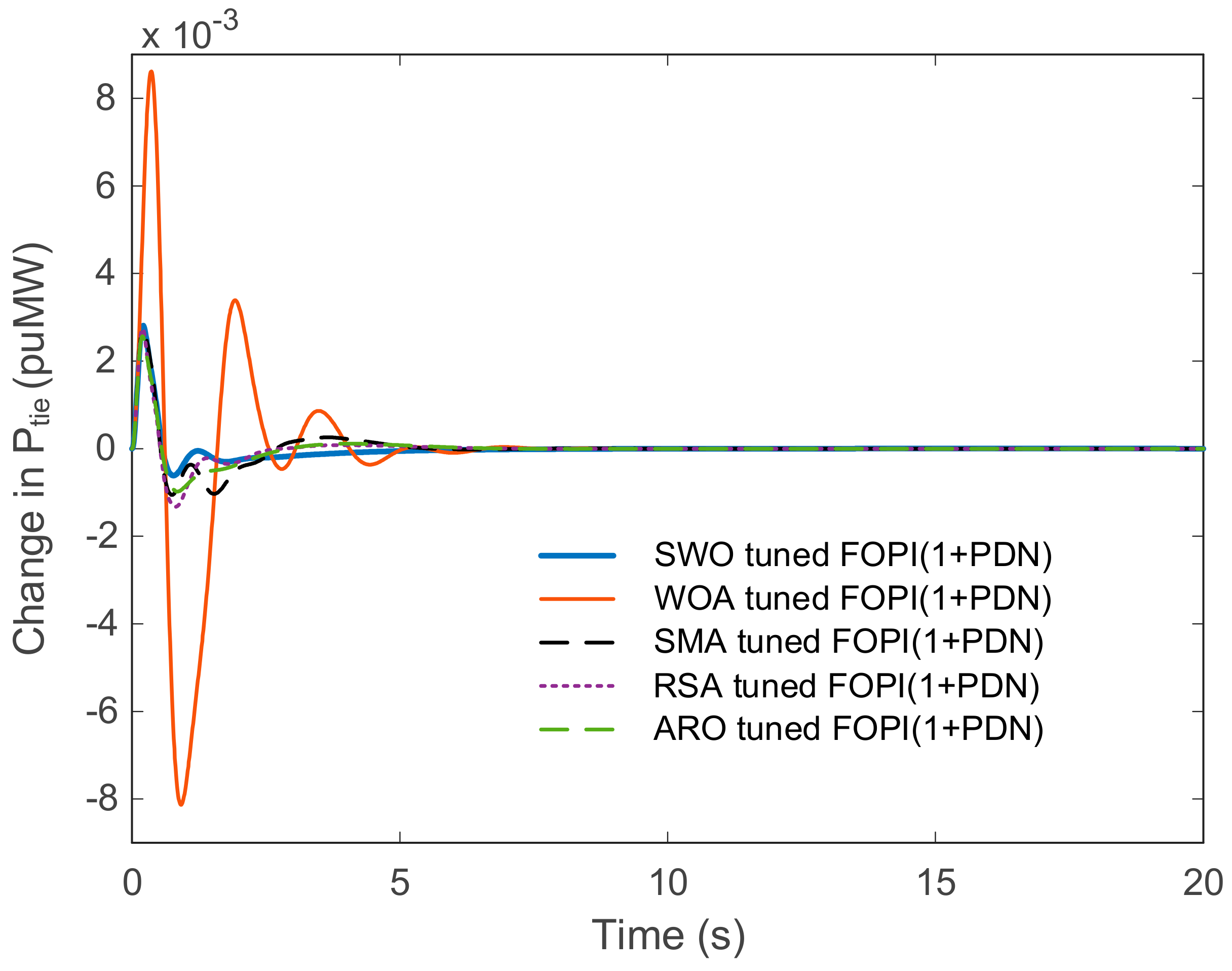
In this scenario, a 10% step change in load is applied simultaneously to both areas of the power system. and represent the step changes in load in Area 1 and Area 2, respectively, both set to 0.1 per unit. This step change is significant as it introduces a sudden demand on the system, challenging the load frequency control mechanisms to restore the balance between supply and demand while maintaining system stability. The system’s response is evaluated by analyzing the frequency deviations in Area 1 () and Area 2 (), as well as the tie-line power change () under the control strategies optimized by the various algorithms.
Figure 6, Figure 7 and Figure 8 illustrate the system’s response in terms of frequency deviations in Area 1 and Area 2 and the tie-line power change. These figures compare the performance of the SWO-tuned FOPI(1+PDN) controller with those tuned by the WOA, SMA, RSA, and ARO.
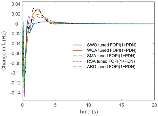
Figure 6.
Frequency deviation in Area 1 in the case of Disturbance I.
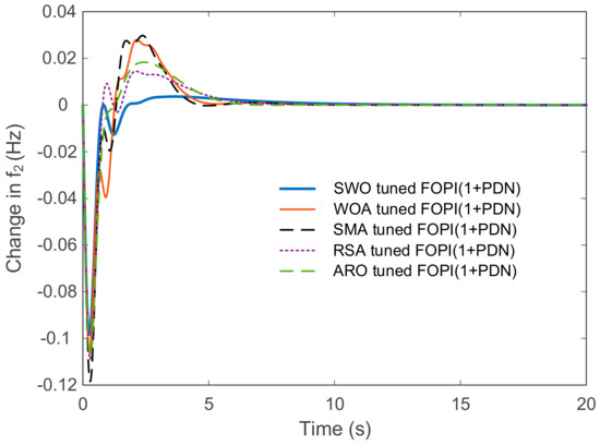
Figure 7.
Frequency deviation in Area 2 in the case of Disturbance I.
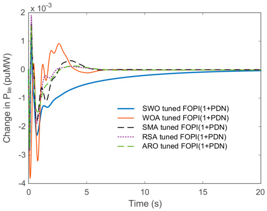
Figure 8.
Tie line power change in the case of Disturbance I.
To ensure a meaningful analysis, settling times were calculated using a 0.05 Hz tolerance band for and , and a 0.01 MW tolerance band for . These tolerance bands are critical for determining when the system has effectively settled after a disturbance. In Table 5, the obtained the undershoot, overshoot, and settling time values are presented via the different approaches in response to Disturbance I. This table offers a quantitative comparison, emphasizing the superior performance of the SWO-tuned FOPI(1+PDN) controller in terms of faster settling times and reduced overshoot and undershoot relative to the other algorithms.
Table 5.
Undershoot, overshoot, and settling time values achieved via different approaches in the case of Disturbance I.
5.2.2. Disturbance II
In the second disturbance scenario, a 10% step change in load is applied exclusively to Area 2. represents the step change in load in Area 2, set to 0.1 per unit. This localized disturbance tests the system’s ability to stabilize the frequency and tie-line power flow in response to a significant change in demand within a single area. The system’s response is analyzed by comparing the frequency deviations in Area 1 () and Area 2 (), as well as the , under the control strategies optimized by the different algorithms.
Figure 9, Figure 10 and Figure 11 provide a visual comparison of the system’s response to this localized disturbance, highlighting the effectiveness of each algorithm in managing the frequency deviations and tie-line power changes. As in the first disturbance scenario, the settling times for , , and were determined using the same tolerance bands (0.05 Hz for frequency deviations and 0.01 MW for tie-line power changes).
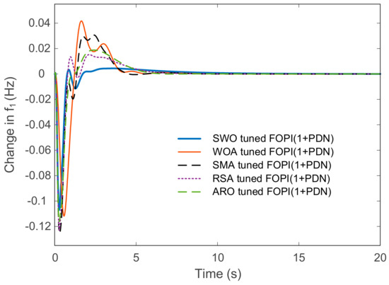
Figure 9.
Frequency deviation in Area 1 in the case of Disturbance II.
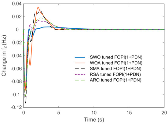
Figure 10.
Frequency deviation in Area 2 in the case of Disturbance II.
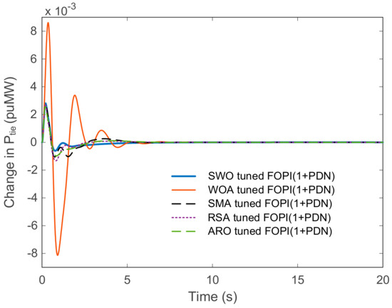
Figure 11.
Tie-line power change in the case of Disturbance II.
Table 6 summarizes the undershoot, overshoot, and settling time values obtained via the different approaches in response to Disturbance II. This table offers a direct comparison of the control strategies, showing how the SWO-tuned FOPI(1+PDN) controller performs relative to the other algorithms under a localized disturbance. The results from these two disturbance scenarios clearly demonstrate the effectiveness of the SWO-tuned FOPI(1+PDN) controller in maintaining system stability. The SWO consistently achieves faster settling times with minimal overshoot and undershoot, outperforming the other algorithms tested. These findings underscore the potential of the SWO to enhance control performance in complex power systems, particularly those involving renewable energy integration.
Table 6.
Undershoot, overshoot, and settling time values achieved via different approaches in the case of Disturbance II.
5.3. Comparisons with Recently Reported Works
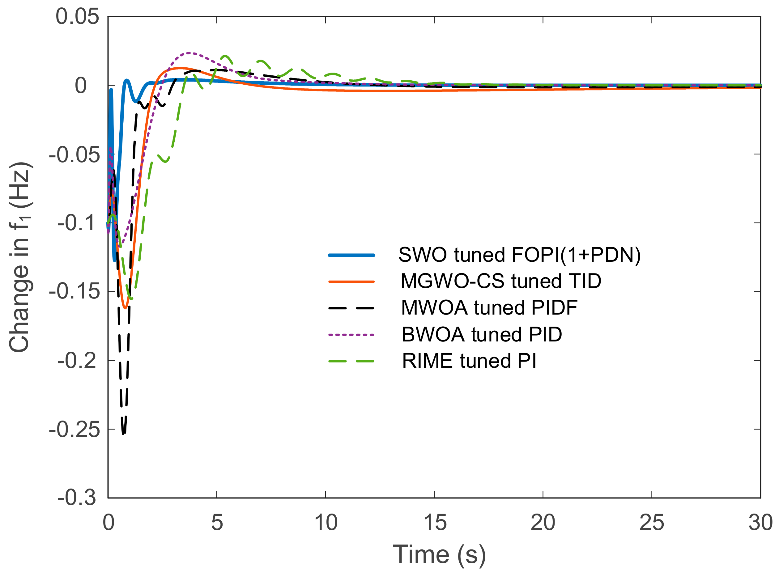
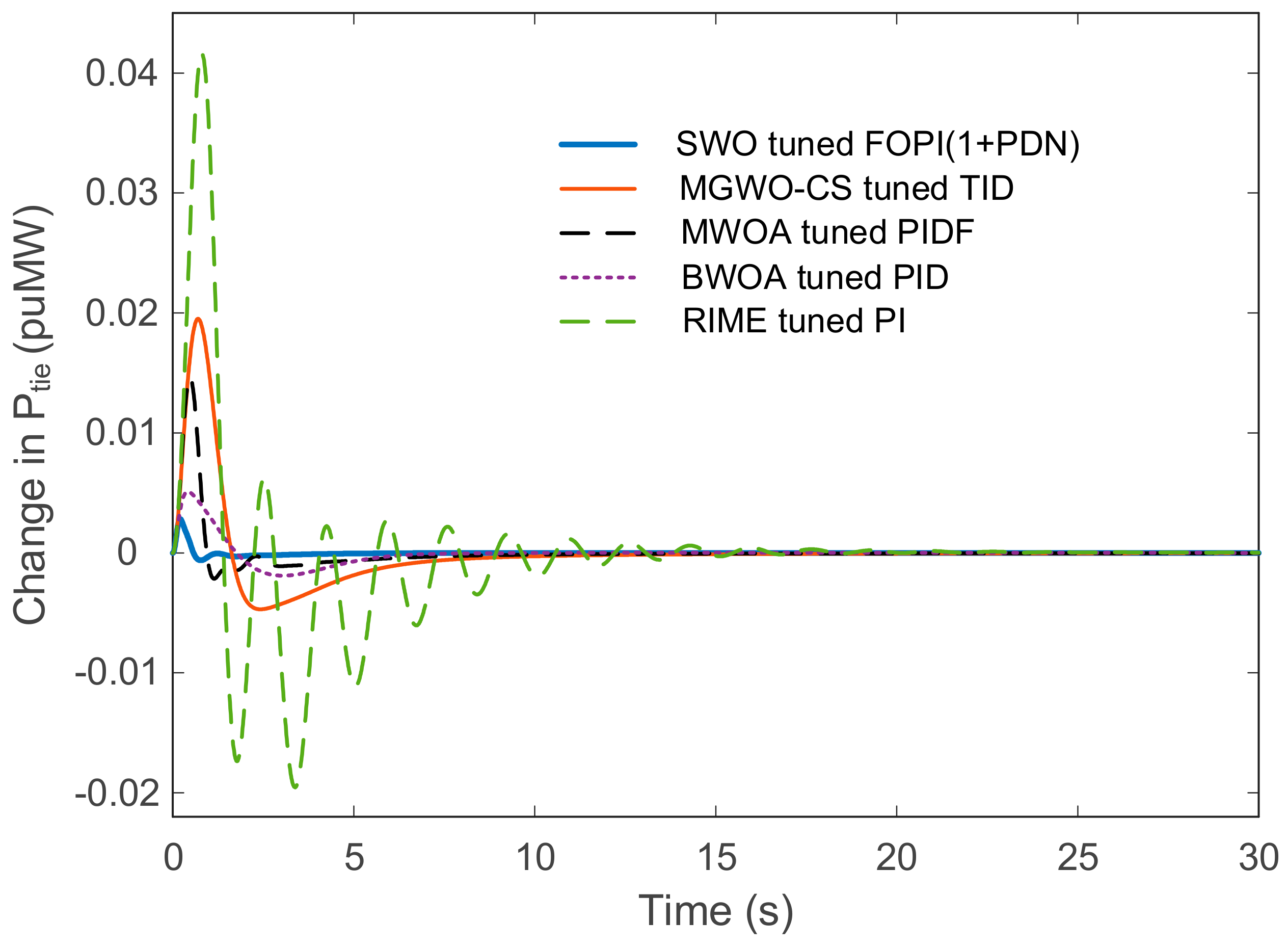
In recent years, various control methods have been developed and optimized using different metaheuristic algorithms. This section compares the performance of the SWO-tuned FOPI(1+PDN) controller with four other control strategies that have been optimized using different algorithms. The control methods considered for comparison are the modified grey wolf optimization–cuckoo search (MGWO-CS)-tuned TID controller [19], the modified whale optimization algorithm (MWOA)-tuned PIDF controller [13], the black widow optimization algorithm (BWOA)-tuned PID controller [21], and the RIME-tuned PI controller [22]. Each of these controllers is represented by the following mathematical equations:
where is a fractional order, which adds flexibility to the controller’s response, and is the proportional gain, which scales the error.
5.3.1. Disturbance I
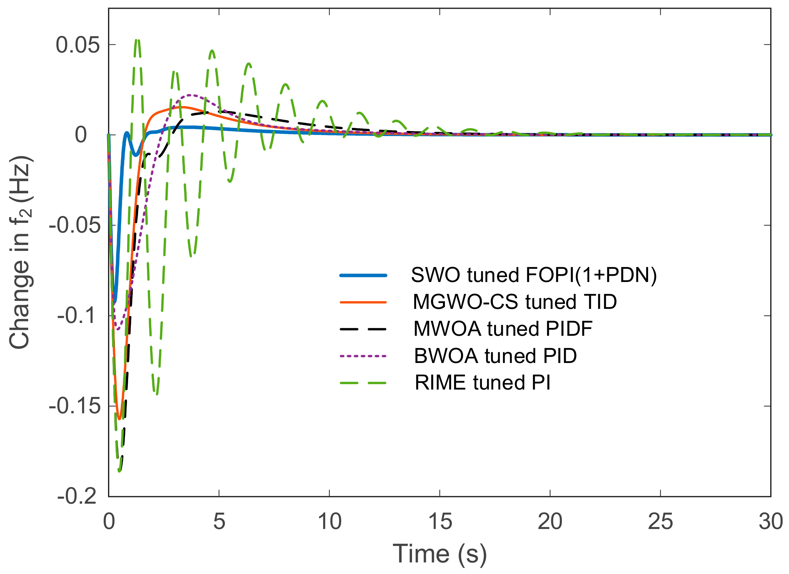
This section compares the performance of the SWO-tuned FOPI(1+PDN) controller with the above-mentioned control strategies under a 10% step change in load applied simultaneously to both areas of the power system (0.1 per unit). The system’s response is evaluated by analyzing the frequency deviations in Area 1 () and Area 2 (), as well as the . Figure 12, Figure 13 and Figure 14 illustrate the system’s response to this disturbance, comparing the performance of the SWO-tuned FOPI(1+PDN) controller with the MGWO-CS-tuned TID, MWOA-tuned PIDF, BWOA-tuned PID, and RIME-tuned PI controllers.
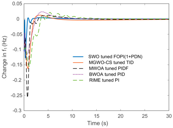
Figure 12.
Frequency deviation comparisons for Area 1 with respect to the reported approaches in the case of Disturbance I.

Figure 13.
Frequency deviation comparisons for Area 2 with respect to the reported approaches in the case of Disturbance I.
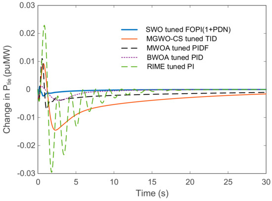
Figure 14.
Tie-line power change with respect to the reported approaches in the case of Disturbance I.
In evaluating the results, the settling times were calculated with a 0.05 Hz tolerance band for and , and a 0.01 MW tolerance band for , ensuring that the system’s response falls within acceptable limits before considering it stable. The undershoot, overshoot, and settling time values achieved by the different approaches in response to Disturbance I are summarized in Table 7. This table provides a quantitative comparison of the control strategies, highlighting the advantages of the SWO-tuned FOPI(1+PDN) controller in achieving quicker settling times and smaller overshoots and undershoots.
Table 7.
Undershoot, overshoot, and settling time values achieved via the reported approaches for Disturbance I.
5.3.2. Disturbance II
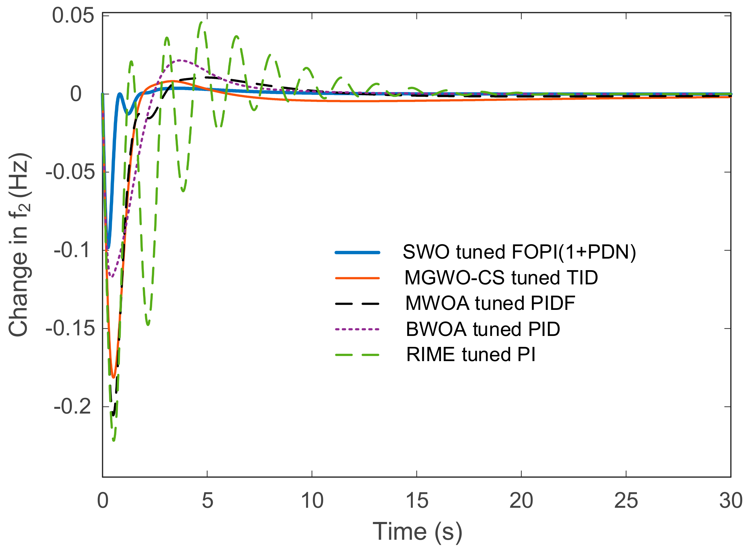
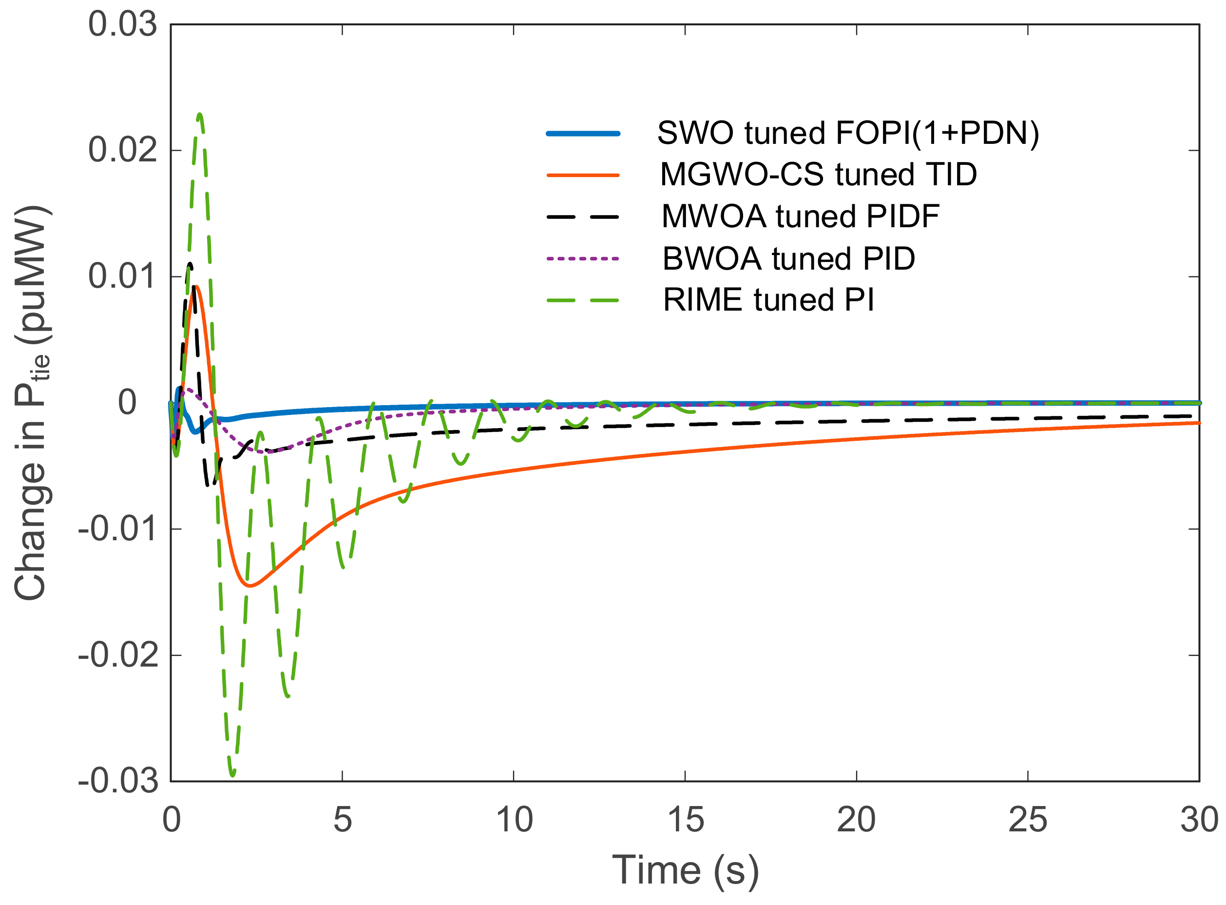
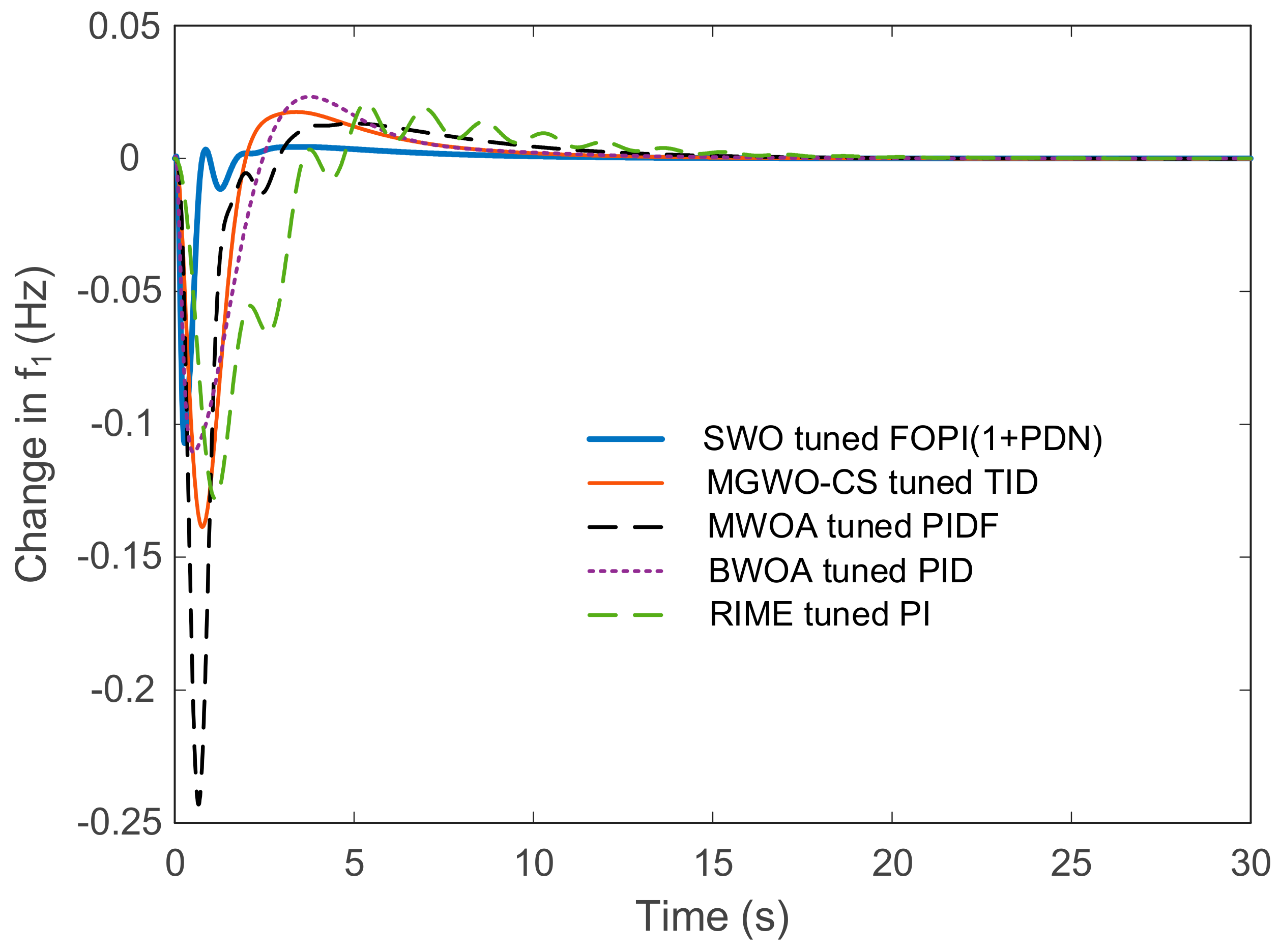
The system’s response is visualized in Figure 15, Figure 16 and Figure 17, which compare the performance of the SWO-tuned FOPI(1+PDN) controller with the MGWO-CS-tuned TID, MWOA-tuned PIDF, BWOA-tuned PID, and RIME-tuned PI controllers. Similar to Disturbance I, the settling times were calculated using the same tolerance bands. Table 8 presents the undershoot, overshoot, and settling time values achieved by the different approaches in response to Disturbance II. This table provides a direct comparison of the control strategies, showing how the SWO-tuned FOPI(1+PDN) controller performs relative to the other algorithms under this localized disturbance. The results from these comparisons demonstrate that the SWO-tuned FOPI(1+PDN) controller consistently provides better performance in terms of settling time, undershoot, and overshoot compared with the recently reported control methods. This highlights the effectiveness of the SWO in optimizing advanced control strategies for load frequency control in complex power systems.
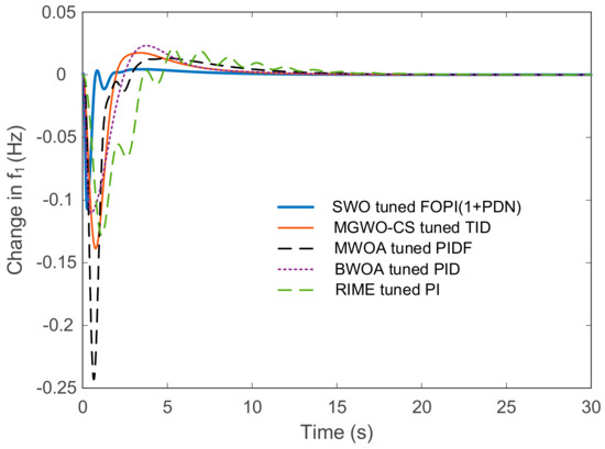
Figure 15.
Frequency deviation comparisons for Area 1 with respect to the reported approaches in the case of Disturbance II.
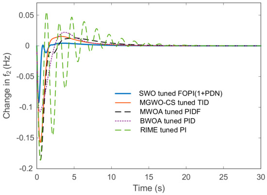
Figure 16.
Frequency deviation comparisons for Area 2 with respect to the reported approaches in the case of Disturbance II.

Figure 17.
Tie-line power change with respect to the reported approaches in the case of Disturbance II.
Table 8.
Undershoot, overshoot, and settling time values achieved via the reported approaches for Disturbance II.
5.4. Comparison of ITAE Performance Metric
In this section, the integral of the time-weighted absolute error (ITAE) performance metric is compared across 20 different control methods, each applied to the same power system parameters. The ITAE metric is a crucial indicator of system performance in load frequency control (LFC), as it emphasizes the importance of minimizing error over time, thereby promoting faster and more stable system responses.
The ITAE values for each control method are summarized below, with the proposed method (SWO-tuned FOPI(1+PDN)) achieving the lowest ITAE value of 0.3281, demonstrating superior performance compared with the other methods. The comparison highlights the effectiveness of the SWO in tuning the FOPI(1+PDN) controller, significantly outperforming other optimization algorithms and control strategies.
The results indicate that the SWO-tuned FOPI(1+PDN) controller not only outperforms all other methods in minimizing the ITAE but does so by a substantial margin. The second-best performance is observed with the MA-tuned PI-PD method, which achieves an ITAE of 0.3379, slightly higher than the proposed SWO-tuned method. Other methods, such as the MA-tuned TID and PID controllers, also perform well, with ITAE values of 0.5979 and 0.7577, respectively, but still fall short of the performance achieved by the SWO. In contrast, traditional and other metaheuristic-based methods, such as the GA-tuned PI and FA-tuned PI controllers, show significantly higher ITAE values, indicating less effective control over the system’s frequency response. These results underscore the critical advantage of using advanced optimization techniques like the SWO for tuning fractional-order controllers in complex power systems. The comparative analysis of ITAE values clearly demonstrates the superiority of the proposed SWO-tuned FOPI(1+PDN) approach, confirming its effectiveness in achieving optimal load frequency control with minimal error over time. This highlights the potential of the SWO as a powerful tool in the design of robust and efficient control systems for power networks with integrated renewable energy sources (see Table 9).
Table 9.
Minimized ITAE values compared with the reported approaches.
Consequently, the searching behavior of the SWO allows the algorithm to explore the solution space more broadly in the early stages, while the pursuit and escape behavior helps refine the search around promising solutions. As the optimization progresses, the SWO dynamically adjusts its exploration and exploitation phases, ensuring that it does not get trapped in local optima, a known limitation of algorithms like the WOA and SMA. Furthermore, the nesting behavior ensures a thorough refinement of the best solutions found, enhancing robustness, particularly in dynamic systems like photovoltaic-integrated multi-area power systems. This mechanism provides the SWO with the ability to respond more effectively to system disturbances, ensuring faster recovery and more stable system performance. In comparison, algorithms such as the RSA and ARO may lack such adaptive mechanisms, leading to less efficient handling of nonlinearities and system uncertainties. The SWO’s dynamic adjustment of search parameters as the optimization progresses allows it to better navigate the complex, multi-modal optimization landscape inherent in LFC problems.
5.5. Qualitative Discussion
The simulation results presented in this study highlight the significant improvements achieved by the SWO-tuned FOPI(1+PDN) controller for LFC in a PV-integrated two-area power system. Beyond the numerical outcomes, the following qualitative insights into the performance of the proposed control strategy further validate its effectiveness and real-world applicability.
The SWO-tuned FOPI(1+PDN) controller demonstrated superior performance across key metrics such as settling time, overshoot, and undershoot when compared with other optimization algorithms and control techniques, including the WOA, SMA, RSA, and ARO. The quicker settling times and reduced frequency deviations observed in the two-area power system underscore the controller’s ability to maintain system stability even under varying disturbance scenarios. This is particularly crucial in modern power systems, where the variability in renewable energy sources, such as PV power, can introduce significant instability. By minimizing frequency fluctuations and ensuring faster system recovery, the proposed controller contributes to enhanced reliability and resilience in real-world power systems.
The findings hold significant practical implications, especially in the context of renewable energy integration. As power grids continue to incorporate higher shares of renewable sources, maintaining frequency stability becomes increasingly challenging. The SWO-tuned FOPI(1+PDN) controller’s superior performance in frequency regulation positions it as a valuable tool for future power grid management. Specifically, it could be applied in smart grids and microgrids where renewable energy fluctuations are common. In practice, its ability to reduce overshoot and undershoot translates to more stable power delivery and improved system efficiency, which could help reduce the operational costs associated with managing renewable energy intermittency.
While the proposed controller has shown robust performance in simulated environments, several limitations could arise in practical applications. One potential challenge is the computational complexity associated with the SWO algorithm, which might limit its real-time application in large-scale power systems. Although the controller performs well in handling typical system disturbances, more extreme conditions, such as sudden large-scale renewable inputs or severe system faults, may require further adjustments or a more adaptive approach. Future work could explore ways to reduce the computational demands of the SWO algorithm or develop hybrid control strategies that combine the SWO with simpler, real-time optimization techniques.
The scalability of the SWO-tuned FOPI(1+PDN) controller for larger and more complex power systems is another avenue for future research [7,16,31]. Testing the controller on physical testbeds or through hardware-in-the-loop simulations would provide additional insights into its performance in real-time environments. Furthermore, integrating real-world data from actual renewable energy systems could help refine the controller’s tuning process and enhance its adaptability to more dynamic and uncertain power system conditions. Research into hybrid optimization techniques that blend the SWO with other metaheuristic or adaptive algorithms could also extend its application to broader operational scenarios.
6. Conclusions
This study presents a novel approach to LFC in a photovoltaic-integrated two-area power system by employing the SWO to tune a cascaded FOPI controller combined with a PDN controller, denoted as FOPI(1+PDN). The proposed method was rigorously evaluated against various control strategies optimized by other advanced metaheuristic algorithms. The simulation results unequivocally demonstrate that the SWO-tuned FOPI(1+PDN) controller achieves superior performance metrics, particularly in terms of minimizing frequency deviations and tie-line power fluctuations. Notably, the controller exhibits faster settling times and smaller overshoot and undershoot compared with the other methods under both global and localized disturbance scenarios. This superior performance is crucial for maintaining the stability of power systems that incorporate renewable energy sources, which are often characterized by variability and uncertainty. The comparative analysis against recently reported control strategies further underscores the effectiveness of the proposed approach. The SWO-tuned FOPI(1+PDN) controller consistently achieves the lowest ITAE values across a wide range of control methods, highlighting its robustness and efficacy in complex power system environments. The success of the SWO in optimizing the parameters of the FOPI(1+PDN) controller is attributed to its ability to balance exploration and exploitation effectively, ensuring a thorough search of the solution space while avoiding premature convergence. This balance is particularly beneficial in addressing the nonlinear and multi-modal nature of the optimization problem inherent in LFC tasks. Additionally, this work not only advances control strategies for LFC but also demonstrates the potential of the SWO as a versatile tool for complex optimization tasks in dynamic, multi-area power networks.
Looking forward, future research could explore the application of the SWO-tuned controller in larger, more diverse power grids with multiple renewable energy sources. Experimental validation of the proposed method could involve testing the SWO-tuned controller on physical testbeds or hardware-in-the-loop (HIL) simulation platforms to assess its real-time performance. Additionally, the implementation of the controller in small-scale microgrids or pilot renewable energy systems would provide valuable insights into its practical applicability. Hybrid optimization techniques or real-time adaptive control strategies could be investigated to further improve the controller’s performance in real-world, large-scale systems. The integration of artificial intelligence for predictive LFC or enhancing the SWO’s capabilities may also offer exciting avenues for further development.
Author Contributions
Conceptualization, M.A.A.; Methodology, S.E.; Validation, D.I.; Formal analysis, D.I and S.E.; Investigation, S.E. and D.I.; Data curation, D.I and S.E.; Writing—original draft, C.T.; Writing—review & editing, D.I., C.T. and M.A.A.; Visualization, S.E.; Supervision, D.I. and S.E.; Funding acquisition, M.A.A. All authors have read and agreed to the published version of the manuscript.
Funding
This research received no external funding.
Data Availability Statement
All produced data are available within this manuscript.
Conflicts of Interest
The authors declare no conflicts of interest.
References
- Çelik, E.; Öztürk, N.; Houssein, E.H. Influence of energy storage device on load frequency control of an interconnected dual-area thermal and solar photovoltaic power system. Neural Comput. Appl. 2022, 34, 20083–20099. [Google Scholar] [CrossRef]
- Mohamed, E.A.; Ahmed, E.M.; Elmelegi, A.; Aly, M.; Elbaksawi, O.; Mohamed, A.A.A. An optimized hybrid fractional order controller for frequency regulation in multi-area power systems. IEEE Access 2020, 8, 213899–213915. [Google Scholar] [CrossRef]
- Sati, M.M.; Kumar, D.; Singh, A.; Raparthi, M.; Alghayadh, F.Y.; Soni, M. Two-Area Power System with Automatic Generation Control Utilizing PID Control, FOPID, Particle Swarm Optimization, and Genetic Algorithms. In Proceedings of the 2024 Fourth International Conference on Advances in Electrical, Computing, Communication and Sustainable Technologies (ICAECT), Bhilai, India, 11–12 January 2024. [Google Scholar]
- Yan, Z.; Xu, Y. A multi-agent deep reinforcement learning method for cooperative load frequency control of a multi-area power system. IEEE Trans. Power Syst. 2020, 35, 4599–4608. [Google Scholar] [CrossRef]
- Ali, H.H.; Kassem, A.M.; Al-Dhaifallah, M.; Fathy, A. Multi-verse optimizer for model predictive load frequency control of hybrid multi-interconnected plants comprising renewable energy. IEEE Access 2020, 8, 114623–114642. [Google Scholar] [CrossRef]
- Acharyulu, B.V.S.; Kumaraswamy, S.; Mohanty, B. Green anaconda optimized DRN controller for automatic generation control of two-area interconnected wind–solar–tidal system. Electr. Eng. 2024, 106, 3543–3558. [Google Scholar] [CrossRef]
- Sharma, M.; Dhundhara, S.; Arya, Y.; Prakash, S. Frequency excursion mitigation strategy using a novel COA optimised fuzzy controller in wind integrated power systems. IET Renew. Power Gener. 2020, 14, 4071–4085. [Google Scholar] [CrossRef]
- Ram Babu, N.; Bhagat, S.K.; Saikia, L.C.; Chiranjeevi, T.; Devarapalli, R.; García Márquez, F.P. A comprehensive review of recent strategies on automatic generation control/load frequency control in power systems. Arch. Comput. Methods Eng. 2023, 30, 543–572. [Google Scholar] [CrossRef]
- Naderipour, A.; Abdul-Malek, Z.; Davoodkhani, I.F.; Kamyab, H.; Ali, R.R. Load-frequency control in an islanded microgrid PV/WT/FC/ESS using an optimal self-tuning fractional-order fuzzy controller. Environ. Sci. Pollut. Res. 2023, 30, 71677–71688. [Google Scholar] [CrossRef] [PubMed]
- Nayak, P.C.; Prusty, R.C.; Panda, S. Adaptive fuzzy approach for load frequency control using hybrid moth flame pattern search optimization with real time validation. Evol. Intell. 2024, 17, 1111–1126. [Google Scholar] [CrossRef]
- Bula Oyuela, C.M. A Reinforcement Learning Based Load Frequency Control for Power Systems Considering Nonlin-Earities and Other Control Interactions. Ph.D. Thesis, Universidad Nacional de Colombia, Bogotá, Colombia, 2024. [Google Scholar]
- Chen, X.; Zhang, M.; Wu, Z.; Wu, L.; Guan, X. Model-free load frequency control of nonlinear power systems based on deep reinforcement learning. IEEE Trans. Ind. Inform. 2024, 20, 6825–6833. [Google Scholar] [CrossRef]
- Khadanga, R.K.; Kumar, A.; Panda, S. A novel modified whale optimization algorithm for load frequency controller design of a two-area power system composing of PV grid and thermal generator. Neural Comput. Appl. 2020, 32, 8205–8216. [Google Scholar] [CrossRef]
- Gharehchopogh, F.S.; Gholizadeh, H. A comprehensive survey: Whale Optimization Algorithm and its applications. Swarm Evol. Comput. 2019, 48, 1–24. [Google Scholar] [CrossRef]
- Li, S.; Chen, H.; Wang, M.; Heidari, A.A.; Mirjalili, S. Slime mould algorithm: A new method for stochastic optimization. Future Gener. Comput. Syst. 2020, 111, 300–323. [Google Scholar] [CrossRef]
- Sharma, M.; Saxena, S.; Prakash, S.; Dhundhara, S.; Arya, Y. Frequency stabilization in sustainable energy sources integrated power systems using novel cascade noninteger fuzzy controller. Energy Sources Part A Recover. Util. Environ. Eff. 2022, 44, 6213–6235. [Google Scholar] [CrossRef]
- Abualigah, L.; Abd Elaziz, M.; Sumari, P.; Geem, Z.W.; Gandomi, A.H. Reptile Search Algorithm (RSA): A nature-inspired meta-heuristic optimizer. Expert Syst. Appl. 2022, 191, 116158. [Google Scholar] [CrossRef]
- Abd-Elazim, S.M.; Ali, E.S. Load frequency controller design of a two-area system composing of PV grid and thermal generator via firefly algorithm. Neural Comput. Appl. 2018, 30, 607–616. [Google Scholar] [CrossRef]
- Khadanga, R.K.; Kumar, A.; Panda, S. A modified grey wolf optimization with cuckoo search algorithm for load frequency controller design of hybrid power system. Appl. Soft Comput. 2022, 124, 109011. [Google Scholar] [CrossRef]
- Khadanga, R.K.; Kumar, A.; Panda, S. A hybrid shuffled frog-leaping and pattern search algorithm for load frequency controller design of a two-area system composing of PV grid and thermal generator. Int. J. Numer. Model. Electron. Netw. Devices Fields 2020, 33, 2694. [Google Scholar] [CrossRef]
- Dahiya, P.; Saha, A.K. Frequency regulation of interconnected power system using black widow optimization. IEEE Access 2022, 10, 25219–25236. [Google Scholar] [CrossRef]
- Ekinci, S.; Can, Ö.; Ayas, M.; Izci, D.; Salman, M.; Rashdan, M. Automatic generation control of a hybrid PV-reheat thermal power system using RIME algorithm. IEEE Access 2024, 12, 26919–26930. [Google Scholar] [CrossRef]
- Wang, L.; Cao, Q.; Zhang, Z.; Mirjalili, S.; Zhao, W. Artificial rabbits optimization: A new bio-inspired meta-heuristic algorithm for solving engineering optimization problems. Eng. Appl. Artif. Intell. 2022, 114, 105082. [Google Scholar] [CrossRef]
- Andic, C.; Ozumcan, S.; Varan, M.; Ozturk, A. A Novel Sea Horse Optimizer Based Load Frequency Controller for Two-Area Power System with PV and Thermal Units. Int. J. Robot. Control. Syst. 2024, 4, 606–627. [Google Scholar] [CrossRef]
- Shangguan, X.-C.; Zhang, C.-K.; He, Y.; Jin, L.; Jiang, L.; Spencer, J.W.; Wu, M. Robust load frequency control for power system considering transmission delay and sampling period. IEEE Trans. Ind. Inform. 2020, 17, 5292–5303. [Google Scholar] [CrossRef]
- Abdel-Basset, M.; Mohamed, R.; Jameel, M.; Abouhawwash, M. Spider wasp optimizer: A novel meta-heuristic optimization algorithm. Artif. Intell. Rev. 2023, 56, 11675–11738. [Google Scholar] [CrossRef]
- Cavdar, B.; Sahin, E.; Sesli, E.; Akyazi, O.; Nuroglu, F.M. Cascaded fractional order automatic generation control of a PV-reheat thermal power system under a comprehensive nonlinearity effect and cyber-attack. Electr. Eng. 2023, 105, 4339–4360. [Google Scholar] [CrossRef]
- Almasoudi, F.M.; Bakeer, A.; Magdy, G.; Alatawi, K.S.S.; Shabib, G.; Lakhouit, A.; Alomrani, S.E. Nonlinear coordination strategy between renewable energy sources and fuel cells for frequency regulation of hybrid power systems. Ain Shams Eng. J. 2024, 15, 102399. [Google Scholar] [CrossRef]
- Mohamed, E.A.; Braik, M.S.; Al-Betar, M.A.; Awadallah, M.A. Boosted Spider Wasp Optimizer for High-dimensional Feature Selection. J. Bionic Eng. 2024, 21, 2424–2459. [Google Scholar] [CrossRef]
- Davtalab, S.; Tousi, B.; Nazarpour, D. Optimized intelligent coordinator for load frequency control in a two-area system with PV plant and thermal generator. IETE J. Res. 2022, 68, 3876–3886. [Google Scholar] [CrossRef]
- Tumari, M.Z.M.; Ahmad, M.A.; Rashid, M.I.M. A fractional order PID tuning tool for automatic voltage regulator using marine predators algorithm. Energy Rep. 2023, 9, 416–421. [Google Scholar] [CrossRef]

Disclaimer/Publisher’s Note: The statements, opinions and data contained in all publications are solely those of the individual author(s) and contributor(s) and not of MDPI and/or the editor(s). MDPI and/or the editor(s) disclaim responsibility for any injury to people or property resulting from any ideas, methods, instructions or products referred to in the content. |
© 2024 by the authors. Licensee MDPI, Basel, Switzerland. This article is an open access article distributed under the terms and conditions of the Creative Commons Attribution (CC BY) license (https://creativecommons.org/licenses/by/4.0/).