Abstract
A streaming graph is a constantly growing sequence of edges, which forms a dynamic graph that changes with every edge in the stream. An anomalous behavior in a streaming graph can be modeled as an edge or a subgraph that is unusual compared to the rest of the graph. Identifying anomalous behaviors in real time is essential to the early warning of abnormal or notable events. Due to the complexity of the problem, little work has been reported so far to solve the problem. In this paper, we propose Finger-based Higher-order Graph Sketch (FHGS for short), which is an approximate data structure for streaming graphs with linear memory usage, high update speed, and high accuracy and supports both edge and subgraph anomaly detection. FHGS first maps each edge into a matrix based on hash functions, and then counts its frequency in a time window with unique fingerprints for detecting anomalies. Extensive experiments confirm that our approach generate high-quality results compared to baseline methods.
MSC:
68P20
1. Introduction
Streaming graphs are drawing increasing attention in both the academic and industrial communities as many graphs in real applications evolve over time. A streaming graph G is an unbounded sequence of items that arrive at a high speed, and each item indicates an edge between two nodes. Typical examples of streaming graphs include social media streams [], computer network traffic data [], financial trade network [], and author-paper graph []. Streaming graph analysis is gaining importance in various fields due to the natural dynamicity in many real graph applications.
Anomaly detection has wide applications in different fields, such as railway safety inspection in the traffic field [], health monitoring in the medicine field [], spam identification in the communication field [], and so on. In the graph mining task, anomaly detection can be used to find edges or subgraphs that are unusual compared to the rest of the graph. These anomalous edges or anomalous subgraphs often indicate the happening of abnormal or notable events. We next use an example of monitoring the happening of anomalous behavior to illustrate its basic idea.
Example 1: Consider a computer network, where nodes correspond to machines, and each edge represents a timestamped connection from one machine to another. In such a streaming graph, anomalous behavior can be described as an individual or a group of attackers making a large number of connections to some set of targeted machines to restrict accessibility or look for potential vulnerabilities []. These anomalous behaviors can be characterized as edges (i.e., malicious connections) and subgraphs (i.e., malicious patterns) that are unusual compared to the rest of the graph. Detecting both these edge and subgraph anomalies together can provide valuable insights into the structure and behavior of the network.
Challenges: In practice, the large scale and high dynamicity of streaming graph make it both memory- and time-consuming to detect anomalous edges and subgraphs accurately. Conventional machine learning algorithms and deep learning techniques are not suitable for real-time anomaly detection over streaming graphs. For example, Bayesian models [,] and hybrid models [] detect anomalies based on statistical probability, nearest neighbour-based approaches [,], and support vector machine (SVM) [] typically represent real-world objects as feature vectors to detect anomalies. All of these approaches discard the relational information in real-world data, so they cannot be used to detect anomalies over graphs. Generative adversarial networks (GANs) [], graph neural networks (GNNs) [], and other deep learning models [,,] rely heavily on training processes and exhibit high time overhead for large-scale data, so they cannot achieve real-time anomaly detection over streaming graphs. So, it is necessary to design a novel data structure that cannot only store streaming graph data but also support anomaly detection algorithms. Existing graph data structures have limitations on supporting anomaly detection over streaming graphs. The adjacency matrix and adjacency list are two traditional graph data structures. However, the adjacency matrix has high memory costs and is not applicable to store large-scale streaming data. On the other hand, the adjacency list has high time costs and is not suitable for storing frequently updated streaming data. Graph summarization techniques can map the graph to the rows and columns of a matrix and preserve the topological information of the graph, which effectively improves the real-time processing ability of streaming graphs. A lot of data structures with graph summarization techniques have been proposed for streaming graphs, such as Count-Min (CM) sketch [], gSketch [], TCM [], gMatrix [], H-CMS [], and GSS []. However, these prior structures either support limited graph algorithms or have poor accuracy. Specifically, CM sketch and gSketch cannot query the topology of the graph, and TCM and gMatrix support the topology query but have poor accuracy. Though H-CMS extends the CM sketch from a two-dimensional structure to a high-order structure, it has poor storage and query accuracy for a large number of hash collisions. GSS proposes fingerprint technology to improve query accuracy, but it cannot directly be used to solve the anomaly detection problem.
Our solution: In this paper, we propose a novel graph data structure, Finger-based Higher-order Graph Sketch (FHGS for short), which can compress the graph node into the rows and columns of a matrix by using hash functions and can uniquely identify the edges in the graph to improve the storage accuracy by using fingerprint technology. Most importantly, it can preserve the topological information of the graph to support graph algorithms. Then, we propose two edge anomaly detection methods, FHGS-EdgeG and FHGS-EdgeL, and two subgraph anomaly detection methods, FHGS-Graph and FHGS-GraphK, based on our proposed FHGS. These four approaches can detect anomalous edges and subgraphs over streaming graphs, respectively, in near real time.
Contributions: The main contributions of our paper are as follows: (1) We propose FHGS, a novel data structure for streaming graphs. It can store streaming graph data under a constant time and space and achieve high accuracy. Most importantly, it preserves the topological information of the graph and can support subsequent graph algorithms. (2) We propose four approaches based on FHGS to detect anomalous edges and subgraphs over streaming graphs in near real time within constantly updated time and memory. And (3) a large number of experiments demonstrate that our methods outperform state-of-the-art anomaly detection methods on three real-world datasets.
The rest of this paper is organized as follows: Section 2 presents the related work. Section 3 describes the research problem. Section 4 presents the data structure. Section 5 and Section 6 describe the anomaly detection algorithms about edges and subgraphs, respectively. Section 7 analyzes the experimental results on three datasets. Section 8 provides the summary of this work.
2. Related Work
Many reviews have been conducted on the graph-based anomaly detection problem in the last few years [,,,,]. In this section, we briefly provide an introduction to prior works.
2.1. Graph Data Structure
Traditional methods for graph storage can be divided into two kinds according to underlying implementation principles. The first kind is native graph storage, which uses a graph prototype to organize and manage data, mainly including adjacency matrix, adjacency list, Neo4j [], and gStore [].This kind has a strong traversal capability and high query efficiency, but it is not suitable for frequently updating scenarios. The second kind of graph storage is based on the relationship model, which uses relational database to store the triplet data of the graph, such as 3store [], SW-Store [], RDF-3X [], and Hexastore []. This kind can update the data in real time but has high query costs.
2.2. Edge Anomaly Detection
The method for anomaly detection on the edge stream was initially proposed by Sharma [], which established a data-driven structured model to define the edges that deviate from the expected structural pattern as anomalies. However, this approach has a poor generalization ability due to the constraints of empirical indicators. Deep learning techniques were employed to detect edge anomaly in Yu et al. []. Moreover, Aggarwal et al. [] proposed a network division method to detect anomaly. These two methods have high time costs and cannot achieve real-time edge anomaly detection. Eswaran et al. [] proposed a principle random algorithm to score the arriving edges according to an anomaly scoring function, while this method is only applicable to specific scenarios and is not scalable.
2.3. Subgraph Anomaly Detection
Akoglu et al. [] proposed a self-centered algorithm that focused on the derived subgraph formed by neighbors around a single node and found subgraph anomalies through a large number of numerical features extracted from the subgraph. Ji et al. [] divided the dynamic graph into a sequence of snapshots to detect anomalies between any two snapshots. These two methods are mainly for static graphs or snapshots. Community-based [] and clustering-based [] anomaly detection methods are both used to detect subgraph anomalies, but they are only suitable for specific scenarios. Eswaran et al. [] defined anomalies as large dense subgraphs that suddenly appear or disappear and proposed the spotlight algorithm for anomaly detection. However, this approach is time-intensive when processing large-scale graphs.
3. Problem
A streaming graph G consists of an unbounded sequence of items, denoted by . Each arriving item is a directed edge represented as , where u represents the source node, v represents the destination node, w is the edge weight, and t is the time edge arrived. Thus, the edge streaming sequence forms a directed graph that changes with the arrival of every item , where V and E denote the set of nodes and the set of edges in the graph, respectively.
Definition 1
(Graph Stream Summarization). Given a streaming graph G, the graph stream summarization problem concerns designing a compact data structure to represent the streaming graph, where the following conditions hold: (1) The space cost of is ; (2) changes with each new arriving data item in the streaming graph, and the time complexity of updating should be as small as possible; and (3) supports various queries over the streaming graph G with small and controllable errors.
In order to reduce the storage scale of the streaming graph, we use summarization to compress the data. The summarization of graph is a smaller graph satisfying and , where a hash function is used to map each node v in G into a node in . Nodes with the same hash value are compressed into one node in , and the edges between them are also compressed together.
Figure 1 shows an example of graph G and its summarization . In this example, we set the value range of the hash function as [0,32). Nodes c and e are mapped to the same node with a hash value of 5 in . The weight of edge is 3 in , which is the sum of the weight of edge and edge in G.
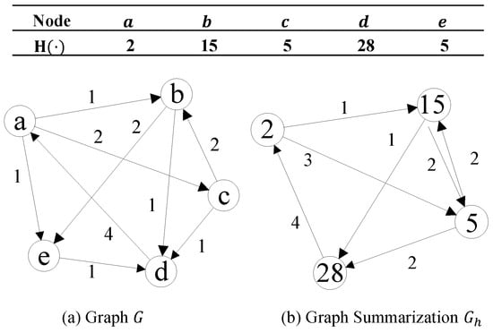
Figure 1.
Graph and summarization.
Thus, given graph , the graph stream summarization problem is to design a data structure to store the summarization , and we call such a data structure as sketch.
In reality, a lot of activities are associated with graph anomalies. For example, the intrusion attacks in computer networks [], the spread of false information in social networks [], and the sudden collaboration between scholars of different fields in academic networks [] can be modeled as edge anomalies. Moreover, behaviors like group fraud in financial networks [] and coordinated attacks in computer systems [] can be represented as subgraph anomalies. Both edge anomaly and subgraph anomaly will lead to a large number of connections between nodes, which makes the graph suddenly denser.
As the definition of anomaly is scenario-related, in this paper, we focus on detecting edges and subgraphs that make the graph dense. Further, the graph sketch preserves the topological information of the graph, so a dense graph can be translated into a dense matrix in the sketch structure. So, we define the edge anomaly and subgraph anomaly as follows.
Definition 2
(Edge anomaly). Given an edge, we store it into the sketch structure; if the edge makes a submatrix dense, then it is an anomalous edge.
Definition 3
(Subgraph anomaly). Given a subgraph, we store it into the sketch structure; if the subgraph makes a submatrix dense, then it is an anomalous subgraph.
We later use submartix density and likehood to measure the degree of a matrix to be dense (see Section 5). Based on the above, we can transform the anomaly detection problem within a network into a dense submatrix search problem in the sketch structure. The desired aims of our paper are as follows:
- Storing streaming graph data: Given a streaming graph, design a data structure with graph summarization techniques to store graph data quickly and satisfy accuracy requirement under constant space and time.
- Detecting anomalous edges: Given an edge, store it into the designed data structure and determine whether the edge is a part of a dense submatrix within constant memory and processing time.
- Detecting anomalous subgraphs: Given a subgraph (consisting of edges arrived over a period of time), store it into the designed data structure and determine the presence of a dense submatrix within constant memory and processing time.
Frequently used notations in our paper are outlined in Table 1.

Table 1.
Notations.
4. Finger-Based Higher-Order Graph Sketch
In this section, inspired by Gou et al. [], we propose FHGS, a novel data structure, which can store streaming graph data under constant time and space and satisfy the accuracy requirement. Most importantly, FHGS can support subsequent graph algorithms. Both theoretical analysis and case illustration show the effectiveness of our approach.
4.1. FHGS: Basic Version
The basic version of FHGS uses a size of in matrix X to store the edges in and can distinguish these edges by fingerprints. For each node in , we define the node address as follows:
Define the node fingerprint as follows:
where M is the value range of the hash function, F is the value range of the fingerprint, and m is the order of the matrix X.
Each edge in is mapped to a cell in row and column of the matrix X. If the cell is empty, we store the fingerprint pair and weight information into the position. If it is not empty, we compare the fingerprint pair information of them. If they are the same, we add the weight to the existing one; otherwise, it means that the position is already occupied by other edges, and a storage collision occurs.
Figure 2 shows the basic version of FHGS for the in Figure 1. Here, we set and . The nodes and their corresponding hash values, addresses, and fingerprints are shown in the table. In this example, the edge is not stored normally because of the collision with edge .
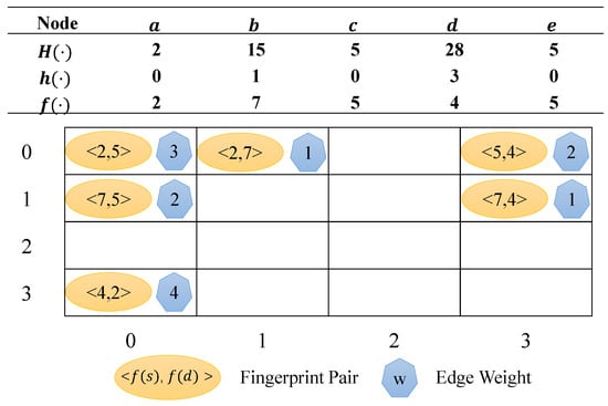
Figure 2.
Basic version of FHGS.
4.2. FHGS: Optimization Strategy
In order to solve the storage collision problem shown above, we introduce a position-resetting strategy to optimize the FHGS structure.
For each node in , we generate a sequence of addresses for it. Thus, a node has r addresses, and an edge has storable positions. If a position is occupied by other edges, it can look for the next position according to the address sequence.
An example of the position-resetting strategy is shown in Figure 3. A node has two addresses, and an edge has four storable positions. In this example, the cells and have been occupied, so the edge can be stored in two remaining empty cells. If we set row-first order when selecting the position, then the edge will be stored in .
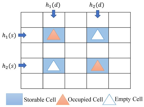
Figure 3.
Position-resetting strategy.
We use the linear congruence method [] to generate a linear congruence random sequence by choosing an appropriate parameter a, small prime b, and a module p, then
We generate the address sequence as follows:
Khan et al. [] confirms that the address sequence generated using the linear congruence method is random and independent without duplicate elements.
Apart from fingerprint pair and weight information, we also store an index pair in the cell, which indicates the order of this cell in the address sequence. Figure 4 shows an example of optimized FHGS based on Figure 2. Here, we set and . The edge are stored properly due to the position-resetting strategy.
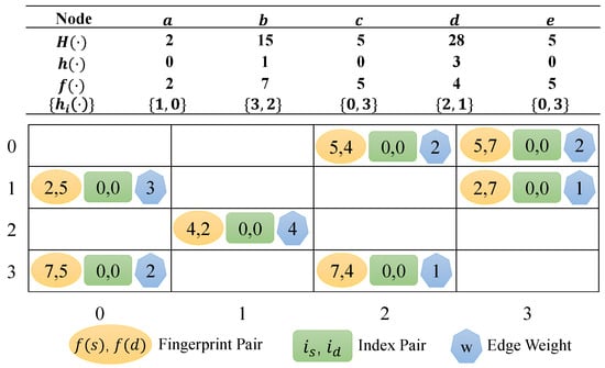
Figure 4.
Optimized FHGS.
The position-resetting strategy solves the collision by providing r addresses for a node. Thus, each edge can find the storage position in matrix X by setting the appropriate r value.
4.3. FHGS: Higher-Order Extension
In order to further improve the accuracy, we extend the sketch to multiple layers. We extend the two-dimensional basic version of FHGS to a higher-order structure by using different hash functions.
Figure 5 shows an example of a k-layer graph summarization with k different hash functions. For each edge in G, different hash functions compress it to corresponding graph summarizations, and we report the minimum weight value over all layers as the accurate result.
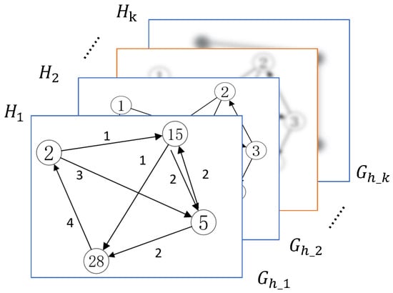
Figure 5.
k-layer graph summarization.
The complete structure of FHGS is shown in Figure 6, which consists of k matrices, and each matrix stores the corresponding graph summarization in Figure 5.
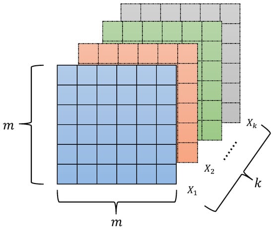
Figure 6.
FHGS structure.
When a new edge of G arriving, FHGS stores the edge as follows:
- Map it to in the graph summarization by using hash function and record the weight w;
- Calculate the fingerprints of the source node , destination node , and the address sequences ,;
- Store the edge information to a cell in matrix X. Check the positions with addresses one by one. For a position , if the cell is empty, store the information into it and end up traversal. If the cell is not empty, compare the fingerprint pair and index pair stored in the cell with the ones of the edge; if both of them are equal, add w to the weight in the cell, and end up traversal. Otherwise, continue to check next position.
- When all positions are occupied, randomly select one of the positions as the storage position of the edge, add the weight w to the existing weight of the cell, and assign the updated weight to the edge. This occurs in memory-constrained conditions, and the error is acceptable.
Proposition 1.
FHGS has memory cost and constantly updating speed. The storage of graph summarization in the data structure is accurate, and the hash collision rate is controllable.
Proof.
FHGS stores, at most, edges in the graph, so the memory complexity is . When storing an edge, it mostly traverses positions. In a k-layer structure, it costs a total of , which is a constant, so the updating time complexity is . For two edges , in , the weights of them are added up if and only if and , which means and are the same edge in . So, the storage of in FHGS is accurate. The collision errors only exist in the hash procedure. We use to represent the probability of edge collision, which means given an edge e, there is at least one satisfying . So, the probability of no collisions is . We assume there are edges in G; for an edge , there are D edges connecting with e. The value range of hash function is M. For an edge that is not connected to e, if the edge collides with e, it means both nodes of the edge have collision. Thus, the probability of this is . The total probability of edges have no collisions with e is . For an edge that is connected to e, if the edge collides with e, it means one of the two nodes has collision. The probability of this is . The total probability of D edges have no collisions with e is . So, the probability of no edges have collisions with e is . For a graph with , we set , so . According to the above formula, the accurate rate is . For the structures which use the adjacent matrix to store , there is , so the accurate rate is . So, the hash collision rate is controllable, and the accuracy of FHGS is much higher than existing structures. □
5. Edge Anomaly Detection
In this section, we propose two edge anomaly detection algorithms based on the FHGS data structures, FHGS-EdgeG and FHGS-EdgeL, which search the dense submatrix from global and local views, respectively.
5.1. FHGS-EdgeG
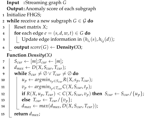
The FHGS-EdgeG (described in Algorithm 1) searches a global dense submatrix on FHGS and outputs the submatrix density as the anomaly score of the edge.
Firstly, we initialize the FHGS. The streaming data are time-sensitive which means the data received recently contain more valuable information. In order to reflect the timeliness of the data, we set an attenuation factor and multiply the edge weight in FHGS with at each timestep to reduce the value of outdated information.
Then, we select the cell , where the edge is stored, as the initial submatrix , where and , and calculate the initial submatrix density. In line with Saha’s work [], we define the submatrix density as follows:
Definition 4
(Submatrix Density). Given a matrix X, the density of a submatrix , where and , is expressed as follows:
We iteratively extend the submatrix by selecting row from (or column from ), which has a maximum row (or column) sum in the remaining matrix, adding the row (or column) to (or ) and removing it from (or ) until both and are empty. We calculate the density of current submatrix in each iteration and report the maximum one over all densities.
We take the density as the anomaly score of the edge. A higher score means the edge is more likely in a dense submatrix and thus more likely to be abnormal. In the k-layer FHGS, the final score is the minimum value returned by all layers.
| Algorithm 1: FHGS-EdgeG() |
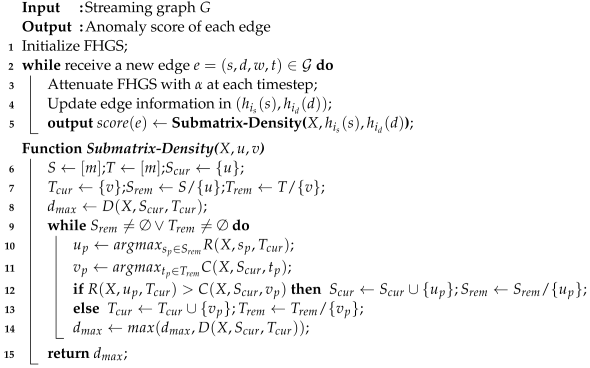 |
Proposition 2.
The time complexity of FHGS-EdgeG is .
Proof.
Submatrix-Density procedure consists of three operations: (a) selecting a row with the maximum sum; (b) selecting a column with the maximum sum; and (c) calculating density. (a) and (b) require at most m steps, so the time complexity is . Calculating the node fingerprint information of a selected row or column requires the most m steps, so (c) has a a time complexity of . The total number of iterations is , so the total time complexity of Submatrix-Density is . Initializing and decaying FHGS needs . When receiving an edge, storing it to FHGS needs the most . Then, Submatrix-Density costs . So, the total time complexity of FHGS-EdgeG is . □
Proposition 3.
The memory complexity of FHGS-EdgeG is .
Proof.
In Submatrix-Density procedure, we use an array of m sizes to remark rows (or columns) and record the sum, and use a list of size to record fingerprints. So, the memory cost of Submatrix-Density is . The FHGS structure costs , and Submatrix-Density costs for k layers. Thus, the total memory complexity of FHGS-EdgeG is . □
5.2. FHGS-EdgeL
The FHGS-EdgeG has high time complexity because of global searching. Thus, we propose FHGS-EdgeL (described in Algorithm 2), which maintains a local dense submatrix on FHGS and outputs the likelihood value of the edge relative to the dense submatrix as the anomaly score of the edge.
Different from FHGS-EdgeG, FHGS-EdgeL randomly selects an element from matrix X as the initial submatrix and updates with a greedy strategy, which aims to keep the submatrix as dense as possible in the subsequent processes.
When an edge arrives, we store it to the position and determine whether to expand the initial submatrix. If the submatrix density increases with the addition of a row (or column) where the edge is located, we add row (or column to (or ). Then, we iteratively select the row (or column) which has the minimum row (or column) sum in the submatrix and remove it from (or ) until the submatrix density no longer increases.
Like density, we define the likelihood of the matrix cell relative to the submatrix , which implies the closeness of the cell to the submatrix.
Definition 5
(Likelihood). Given a matrix X, the likelihood of the index with respect to a submatrix where and , is expressed as follows:
We take the likelihood as the anomaly score of the edge. A higher score means the edge is more likely to be abnormal. In the k-layer FHGS, the final score is the minimum value returned by all layers.
| Algorithm 2: FHGS-EdgeL() |
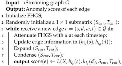 |
Proposition 4.
The time complexity of FHGS-EdgeL is .
Proof.
Initializing and decaying FHGS needs . When receiving an edge, storing it to FHGS needs the most . Expanding and condensing the submatrix both needs the most ; thus, the time complexity of Expand and Condense is . Calculating the likelihood costs . So, the total time complexity of FHGS-EdgeL is . □
Proposition 5.
The memory complexity of FHGS-EdgeL is .
Proof.
The FHGS structure costs . We use an array of m sizes to remark the submatrix information which takes . So, the total memory complexity of FHGS-EdgeL is . □
6. Subgraph Anomaly Detection
In this section, using the FHGS data structure, we propose using FHGS-Graph and FHGS-GraphK to detect subgraph anomaly. FHGS-Graph searches the dense submatrix from the global view. FHGS-GraphK strategically picks up K elements to search the dense submatrix around them.
6.1. FHGS-Graph
The FHGS-Graph (described in Algorithm 3) searches the dense submatrix on FHGS and outputs the submatrix density as the anomaly score of the subgraph.
We divide the streaming graph into subgraphs according to the edge arrival time and defined time window. Then, we reinitialize FHGS when a new subgraph arrives at each time window.
We first take matrix X as the initial submatrix and calculate the initial submatrix density. We then iteratively select a row (or column) with the minimum row (or column) sum in the submatrix and remove the row (or column) from (or ) until the submatrix is empty. In each iteration, we calculate the density of the current submatrix according to Equation (6) and return the maximum density of all submatrices.
| Algorithm 3: FHGS-Graph() |
 |
Proposition 6.
The time complexity of FHGS-Graph is .
Proof.
In the Density procedure, we iteratively delete the rows and columns at the highest times. Selecting the rows (or columns) with the minimum sum and updating sum both take . Calculating density costs . So, the total time complexity of Density is . Initializing FHGS needs . When receiving a subgraph, resetting the matrix needs , updating the edges costs , and Density takes . So, the total time complexity of FHGS-Graph is , where is the number of subgraphs, and is the number of edges in G. □
Proposition 7.
The memory complexity of FHGS-Graph is .
Proof.
In the Density procedure, we use an array of m sizes to remark the rows (or columns) and record the sum, and use a list of sizes to record fingerprints. So, the memory cost of Density is . The FHGS structure costs , and Density costs for k layers. Thus, the total memory complexity of FHGS-Graph is . □
6.2. FHGS-GraphK
Inspired by the idea that the element with a higher weight is more likely to be a part of the dense submatrix, we propose FHGS-GraphK (described in Algorithm 4), which searches dense submatrix around top-K elements in the matrix and returns the submatrix density as the anomaly score of the subgraph.
We iteratively select the largest element in matrix X as the initial submatrix and use the - process in Algorithm 1 to calculate the submatrix density. Then, we remove this element from the matrix after each iteration and continue to select the next largest element until K elements are selected.
| Algorithm 4: FHGS-GraphK() |
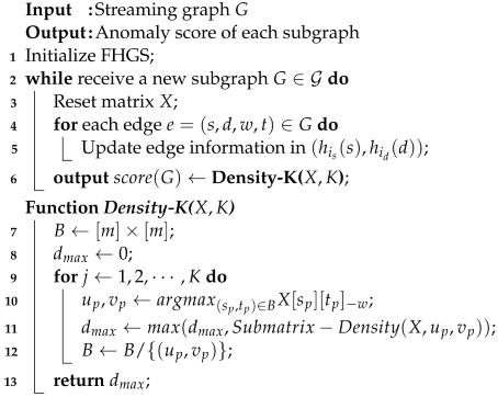 |
Proposition 8.
The time complexity of FHGS-GraphK is .
Proof.
The Density-K procedure is the same as Submatrix-Density, so the time complexity of Density-K is . Other procedures are similar to FHGS-Graph; thus, the total time complexity of FHGS-GraphK is , where is the number of subgraphs, and is the number of edges in G. □
Proposition 9.
The memory complexity of FHGS-GraphK is .
Proof.
The memory complexity of Density-K is . The FHGS structure costs . Thus, the total memory complexity of FHGS-GraphK is . □
7. Experiments
In this section, we evaluate the effectiveness and scalability of the experimental results. All the algorithms were implemented in C++ and Python, run on a PC with an Intel i5 1.6GHz CPU and 8GB memory. We take the Area under the ROC (AUC) and the running time as evaluation metrics. Every quantitative test was repeated for 5 times, and the average is reported.
Datasets: We use three real-life datasets:
- DARPA []: This dataset includes four attack types: DoS (Denial of Service), U2R (User to Root), R2L (Remote to Local), and Probe. It records the IP-IP connection and provides the ground truth. It contains 25K nodes, 4M edges, and 46K timestamps.
- ISCX-IDS2012 []: This dataset simulates intrusion scenarios based on real network traffic and records network activity over a seven-day period. It contains 30k nodes, 1M edges, and 165K timestamps.
- UNSW-NB15 []: This dataset contains a large amount of network traffic data and simulated attack data, covering nine attack types: Fuzzers, Analysis, Backdoors, DoS, Exploits, Generic, Reconnaissance, Shellcode, and Worms. It contains 45 nodes, 1M edges, and 43K timestamps.
Baselines: We implement and compare our algorithms with the below baselines:
- AnoEdge-G and AnoEdge-L []: Two baselines for detecting edge anomalies using the H-CMS data structure.
- MIDAS-R []: The baseline for detecting edge anomalies based on microcluster.
- F-FADE []: The baseline for detecting edge anomalies using frequency factorization.
- FHGS-EdgeG and FHGS-EdgeL: Our methods for detecting edge anomalies.
- AnoGraph and AnoGraph-K []: Two baselines for detecting subgraph anomalies using the H-CMS data structure.
- SPOTLIGHT []: The baseline for detecting subgraph anomalies using a randomized approach.
- ANOMRANK []: The baseline for detecting subgraph anomalies using PageRank score vectors.
- FHGS-Graph and FHGS-GraphK: Our methods for detecting subgraph anomalies.
Parameter settings: For our methods, we fix FHGS layers , hash function range M = 320,000, parameters , and matrix order . We set the number of addresses on DARPA, ISCX-IDS2012, and UNSW-NB15 as 1, 1, and 4, respectively. In edge anomaly detection experiments, we set the attenuation factor on DARPA, ISCX-IDS2012, and UNSW-NB15 as 0.9, 0.96, and 0.98, respectively. In subgraph anomaly detection experiments, on DARPA, ISCX-IDS2012, and UNSW-NB15, we set time window as 15, 30, and 15, fix the edge threshold as 100, and fix . For baselines, we set the layers of H-CMS to 1 in AnoEdge and AnoGraph for fairness and follow other parameter settings, as suggested in previous papers. We conduct a large number of experiments under different parameter settings and choose the most representative parameter values here.
7.1. Experiments on Edge Anomaly Detection
Effectiveness: Table 2 and Figure 7 show the AUC and running time of edge anomaly detection approaches on three datasets. The results show that our approaches outperform on detection accuracy and can achieve the near real-time requirement. Compared to the best prior results, FHGS-EdgeG and FHGS-EdgeL improve the AUC by 1.78% and 0.94% on DARPA, 1.7% and 2.24% on ISCX-IDS2012, and 55.88% and 27.25% on UNSW-NB15, respectively. F-FADE shows a large computation time because it needs to extract patterns for every update. Our approaches have additional time expenses due to the use of position-resetting strategy on the FHGS structure which focuses on improving storage accuracy, even though our approaches can also detect edge anomalies in a small time span. Moreover, since FHGS-EdgeL maintains a local dense submatrix, it is faster than FHGS-EdgeG.
Table 2.
AUC and running time on edge anomaly detection.
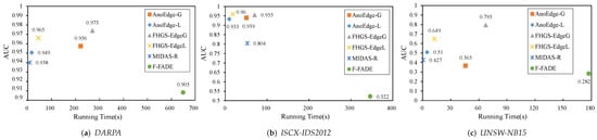
Figure 7.
AUC vs. running time of edge anomaly detection on three datasets.
Scalability: Figure 8a–d plot the running time with an increasing number of edges, FHGS layers, matrix size (), and address sequences, respectively. All of these results imply the scalability of FHGS-EdgeG and FHGS-EdgeL.
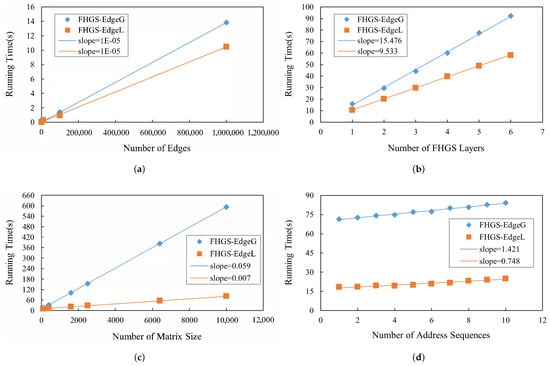
Figure 8.
(a) Scalability with number of edges; (b) scalability with number of FHGS layers; (c) scalability with matrix size; (d) scalability with number of address sequences.
7.2. Experiments on Subgraph Anomaly Detection
Effectiveness: Table 3 and Figure 9 show the AUC and running time of subgraph anomaly detection approaches on three datasets. We can see that our approaches demonstrate superior performance in terms of detection accuracy and can meet near real-time demand. Compared to the best prior results, FHGS-Graph and FHGS-GraphK improve the AUC by 5.46% and 6.07% on DARPA, 5.55% and 5.66% on ISCX-IDS2012, and 3.23% and 3.34% on UNSW-NB15, respectively. ANOMRANK has a low AUC because it is not meant for processing streaming data. SPOTLIGHT has a large computation time due to the randomized searching approach. Although our algorithms take more time, they can also detect subgraph anomalies in near real time.
Table 3.
AUC and running time on subgraph anomaly detection.
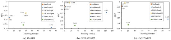
Figure 9.
AUC vs. running time of subgraph anomaly detection on three datasets.
Scalability: Figure 10a–d plot the running time with an increasing number of edges, FHGS layers, matrix size, and K value, respectively. All of these results imply the scalability of FHGS-Graph and FHGS-GraphK.
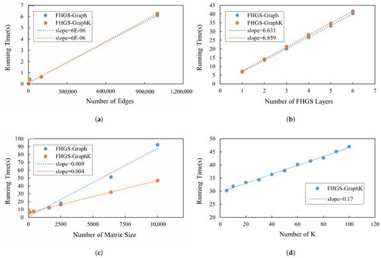
Figure 10.
(a) Scalability with number of edges; (b) scalability with number of FHGS layers; (c) scalability with matrix size; (d) scalability with K.
8. Conclusions
Network anomaly detection is widely used in various real-world scenarios. However, existing methods cannot detect anomalies over streaming graphs quickly and accurately. In this paper, we first propose a higher-order graph data structure, FHGS, which can store streaming graph data under constant time and space with high accuracy and preserve the topological structure of the graph to support graph algorithms. Based on the FHGS structure, we then propose two edge anomaly detection algorithms, FHGS-EdgeG and FHGS-EdgeL, and two subgraph anomaly detection algorithms, FHGS-Graph and FHGS-GraphK. These four algorithms detect anomalies by searching a dense submatrix on the data structure. For edge anomaly detection, FHGS-EdgeG searches the dense submatrix from a global view and has high accuracy, while FHGS-EdgeL maintains the dense submatrix on a local scale and performs better in time complexity. For subgraph anomaly detection, FHGS-Graph searches the dense submatrix on global scale, while FHGS-GraphK strategically picks up K elements to search the dense submatrix around them. The experimental results on the three datasets demonstrate that our methods can detect both edge and subgraph anomalies quickly and accurately compared to state-of-the-art baselines.
Author Contributions
Conceptualization, M.L.; methodology, M.L.; validation, M.L.; writing—original draft preparation, M.L.; supervision, Q.Z. and X.Z. All authors have read and agreed to the published version of the manuscript.
Funding
This research was funded by the National Defense Basic Scientific Research Program under No. WDZC20235250412.
Data Availability Statement
The datasets can be found at https://www.ll.mit.edu/r-d/datasets/1998-darpa-intrusion-detection-evaluation-dataset (accessed on 10 July 2024), https://www.unb.ca/cic/datasets/ids.html (accessed on 10 July 2024) and https://research.unsw.edu.au/projects/unsw-nb15-dataset (accessed on 10 July 2024).
Conflicts of Interest
The authors declare that they have no known competing financial interests or personal relationships that could have appeared to influence the work reported in this paper.
References
- Aggarwal, C.C. (Ed.) An Introduction to Social Network Data Analytics. In Social Network Data Analytics; Springer: Boston, MA, USA, 2011. [Google Scholar]
- Eswaran, D.; Faloutsos, C. SedanSpot: Detecting Anomalies in Edge Streams. In Proceedings of the 2018 IEEE International Conference on Data Mining (ICDM), Singapore, 17–20 November 2018. [Google Scholar]
- Bay, S.; Kumaraswamy, K.; Anderle, M.G.; Kumar, R.; Steier, D.M. Large Scale Detection of Irregularities in Accounting Data. In Proceedings of the 6th International Conference on Data Mining (ICDM’06), Hong Kong, China, 18–22 December 2006. [Google Scholar]
- Sun, J.; Qu, H.; Chakrabarti, D.; Faloutsos, C. Neighborhood formation and anomaly detection in bipartite graphs. In Proceedings of the 5th IEEE International Conference on Data Mining, Houston, TX, USA, 27–30 November 2005. [Google Scholar]
- Liu, R.; Liu, W.; Zheng, Z.; Wang, L.; Mao, L.; Qiu, Q.; Ling, G. Anomaly-GAN: A data augmentation method for train surface anomaly detection. Expert Syst. Appl. 2023, 228, 120284. [Google Scholar] [CrossRef]
- Zhang, Y.M.; Wang, H.; Wan, H.P.; Mao, J.X.; Xu, Y.C. Anomaly detection of structural health monitoring data using the maximum likelihood estimation-based Bayesian dynamic linear model. Struct. Health Monit. 2021, 20, 2936–2952. [Google Scholar] [CrossRef]
- Ma, X.; Wu, J.; Xue, S.; Yang, J.; Zhou, C.; Sheng, Q.Z.; Xiong, H.; Akoglu, L. A Comprehensive Survey on Graph Anomaly Detection with Deep Learning. IEEE Trans. Knowl. Data Eng. 2023, 35, 12012–12038. [Google Scholar] [CrossRef]
- Lippman, R.P.; Cunningham, R.K.; Fried, D.J.; Graf, I.; Kendall, K.R.; Webster, S.E.; Zissman, M.A. Results of the DARPA 1998 offline intrusion detection evaluation. In Proceedings of the Recent Advances in Intrusion Detection, RAID 99 Conference, West Lafayette, IN, USA, 7–9 September 1998. [Google Scholar]
- Sebyala, A.A.; Olukemi, T.; Sacks, L. Active Platform Security through Intrusion Detection Using Naïve Bayesian Network for Anomaly Detection. In Proceedings of the London Communications Symposium 2002, London, UK, 9–10 September 2002. [Google Scholar]
- Grcic, M.; Bevandic, P.; Segvic, S. DenseHybrid: Hybrid Anomaly Detection for Dense Open-Set Recognition. In Proceedings of the European Conference on Computer Vision, Tel Aviv, Israel, 23–27 October 2022. [Google Scholar]
- Hautamaki, V.; Karkkainen, I.; Franti, P. Outlier detection using k-nearest neighbour graph. In Proceedings of the 17th International Conference on Pattern Recognition, Cambridge, UK, 23–26 August 2004. [Google Scholar]
- Bay, S.D.; Schwabacher, M. Mining Distance-Based Outliers in Near Linear Time with Randomization and a Simple Pruning Rule. In Proceedings of the 9th ACM SIGKDD International Conference on Knowledge Discovery and Data Mining, Washington, DC, USA, 24–27 August 2003. [Google Scholar]
- Erfani, S.; Rajasegarar, S.; Karunasekera, S.; Leckie, C. High-dimensional and large-scale anomaly detection using a linear one-class SVM with deep learning. Pattern Recognit. 2016, 58, 121–134. [Google Scholar] [CrossRef]
- Chalapathy, R.; Chawla, S. Deep Learning for Anomaly Detection: A Survey. arXiv 2019, arXiv:1901.03407. [Google Scholar]
- Pang, G.; Shen, C.; Cao, L.; Van Den Hengel, A. Deep Learning for Anomaly Detection: A Review. ACM Comput. Surv. 2022, 54, 1–38. [Google Scholar] [CrossRef]
- Ruff, L.; Kauffmann, J.R.; Vandermeulen, R.A.; Montavon, G.; Samek, W.; Kloft, M.; Dietterich, T.G.; Müller, K.R. A Unifying Review of Deep and Shallow Anomaly Detection. Proc. IEEE 2021, 109, 756–795. [Google Scholar] [CrossRef]
- Cormode, G.; Muthukrishnan, S. An improved data stream summary: The count-min sketch and its applications. J. Algorithms 2005, 55, 58–75. [Google Scholar] [CrossRef]
- Zhao, P.; Aggarwal, C.C.; Wang, M. gSketch: On Query Estimation in Graph Streams. arXiv 2011, arXiv:1111.7167. [Google Scholar] [CrossRef]
- Tang, N.; Chen, Q.; Mitra, P. Graph Stream Summarization: From Big Bang to Big Crunch. In Proceedings of the SIGMOD ’16: Proceedings of the 2016 International Conference on Management of Data, San Francisco, CA, USA, 26 June–1 July 2016. [Google Scholar]
- Khan, A.; Aggarwal, C. Query-friendly compression of graph streams. In Proceedings of the 2016 IEEE/ACM International Conference on Advances in Social Networks Analysis and Mining (ASONAM), San Francisco, CA, USA, 18–21 August 2016. [Google Scholar]
- Bhatia, S.; Wadhwa, M.; Kawaguchi, K.; Shah, N.; Yu, P.S.; Hooi, B. Sketch-Based Anomaly Detection in Streaming Graphs. In Proceedings of the 29th ACM SIGKDD Conference on Knowledge Discovery and Data Mining (KDD), Long Beach, CA, USA, 6–10 August 2023. [Google Scholar]
- Gou, X.; Zou, L.; Zhao, C.; Yang, T. Fast and Accurate Graph Stream Summarization. In Proceedings of the 2019 IEEE 35th International Conference on Data Engineering (ICDE), Macao, China, 8–11 April 2019. [Google Scholar]
- Yu, R.; Qiu, H.; Wen, Z.; Lin, C.; Liu, Y. A Survey on Social Media Anomaly Detection. ACM Sigkdd Explor. Newsl. 2016, 18, 1–14. [Google Scholar] [CrossRef]
- Pourhabibi, T.; Ong, K.L.; Kam, B.H.; Boo, Y.L. Fraud detection: A systematic literature review of graph-based anomaly detection approaches. Decis. Support Syst. 2020, 133, 113303. [Google Scholar] [CrossRef]
- D’Souza, D.J.; Reddy, K.R.U.K. Anomaly Detection for Big Data Using Efficient Techniques: A Review. In Proceedings of the Advances in Artificial Intelligence and Data Engineering, Udupi, India, 23–24 May 2020. [Google Scholar]
- Ranshous, S.; Harenberg, S.; Shen, S.; Samatova, N.F.; Faloutsos, C.; Koutra, D. Anomaly detection in dynamic networks: A survey. Wiley Interdiscip. Rev. Comput. Stat. 2015, 7, 223–247. [Google Scholar] [CrossRef]
- Akoglu, L.; Tong, H.; Koutra, D. Graph based anomaly detection and description: A survey. Data Min. Knowl. Discov. 2015, 29, 626–688. [Google Scholar] [CrossRef]
- Wang, X.; Zou, L.; Wang, C.K.; Peng, P.; Feng, Z.Y. Research on Knowledge Graph Data Management: A Survey (Review). Ruan Jian Xue Bao/J. Softw. 2019, 30, 2139–2174. [Google Scholar]
- Zou, L.; Oezsu, M.T.; Chen, L.; Shen, X.; Huang, R.; Zhao, D. gStore: A graph-based SPARQL query engine. VLDB J. 2014, 23, 565–590. [Google Scholar] [CrossRef]
- Harris, S.; Gibbins, N. 3store: Efficient Bulk RDF Storage. In Proceedings of the 1st International Workshop on Practical and Scalable Semantic Systems (PSSS’03), Sanibel Island, FL, USA, 20 October 2003. [Google Scholar]
- Abadi, D.J.; Marcus, A.; Madden, S.; Hollenbach, K. SW-Store: A vertically partitioned DBMS for semantic web data management (Article). VLDB J. 2009, 18, 385–406. [Google Scholar] [CrossRef]
- Neumann, T.; Weikum, G. The RDF-3X engine for scalable management of RDF data (Article). VLDB J. 2010, 19, 91–113. [Google Scholar] [CrossRef]
- Weiss, C.; Karras, P.; Bernstein, A. Hexastore. Proc. Vldb Endow. 2008, 1, 1008–1019. [Google Scholar] [CrossRef]
- Ranshous, S.; Harenberg, S.; Sharma, K. A Scalable Approach for Outlier Detection in Edge Streams Using Sketch-based Approximations. In Proceedings of the 2016 SIAM International Conference on Data Mining (SDM 2016), Miami, FL, USA, 5–7 May 2016. [Google Scholar]
- Yu, W.; Cheng, W.; Aggarwal, C.C.; Zhang, K.; Chen, H.; Wang, W. NetWalk: A Flexible Deep Embedding Approach for Anomaly Detection in Dynamic Networks. In Proceedings of the KDD ’18: Proceedings of the 24th ACM SIGKDD International Conference on Knowledge Discovery & Data Mining, London, UK, 19–23 August 2018. [Google Scholar]
- Aggarwal, C.C.; Zhao, Y.; Yu, P.S. Outlier detection in graph streams. In Proceedings of the 2011 IEEE 27th International Conference on Data Engineering, Hannover, Germany, 11–16 April 2011. [Google Scholar]
- Akoglu, L.; McGlohon, M.; Faloutsos, C. OddBall: Spotting Anomalies in Weighted Graphs. In Proceedings of the Pacific-Asia Conference on Knowledge Discovery and Data Mining (PAKDD 2010), Hyderabad, India, 21–24 June 2010. [Google Scholar]
- Ji, T.; Yang, D.; Gao, J. Incremental Local Evolutionary Outlier Detection for Dynamic Social Networks. In Proceedings of the European Conference on Machine Learning and Principles and Practice of Knowledge Discovery in Databases, Prague, Czech Republic, 23–27 September 2013. [Google Scholar]
- Chen, Z.; Hendrix, W.; Samatova, N. Community-based anomaly detection in evolutionary networks (Article). J. Intell. Inf. Syst. 2012, 39, 59–85. [Google Scholar] [CrossRef]
- Manzoor, E.; Milajerdi, S.M.; Akoglu, L. Fast Memory-efficient Anomaly Detection in Streaming Heterogeneous Graphs. In Proceedings of the KDD ’16: Proceedings of the 22nd ACM SIGKDD International Conference on Knowledge Discovery and Data Mining, San Francisco, CA, USA, 13–17 August 2016. [Google Scholar]
- Eswaran, D.; Faloutsos, C.; Guha, S.; Mishra, N. SpotLight: Detecting Anomalies in Streaming Graphs. In Proceedings of the KDD ’18: Proceedings of the 24th ACM SIGKDD International Conference on Knowledge Discovery & Data Mining, London, UK, 19–23 August 2018. [Google Scholar]
- Gupta, M.; Gao, J.; Sun, Y.; Han, J. Integrating community matching and outlier detection for mining evolutionary community outliers. In Proceedings of the KDD ’12: Proceedings of the 18th ACM SIGKDD International Conference on Knowledge Discovery and Data Mining, Beijing, China, 12–16 August 2012. [Google Scholar]
- Heard, B.N.A.; Weston, D.J.; Platanioti, K.; Hand, D.J. Bayesian anomaly detection methods for social networks. Ann. Appl. Stat. 2010, 4, 645–662. [Google Scholar] [CrossRef]
- L’Ecuyer, P. Tables of linear congruential generators of different sizes and good lattice structure. Math. Comput. 1999, 68, 249–260. [Google Scholar] [CrossRef]
- Khuller, S.; Saha, B. On Finding Dense Subgraphs. In Proceedings of the Automata, Languages and Programming, Rhodes, Greece, 5–12 July 2009. [Google Scholar]
- Shiravi, A.; Shiravi, H.; Tavallaee, M.; Ghorbani, A.A. Toward developing a systematic approach to generate benchmark datasets for intrusion detection. Comput. Secur. 2012, 31, 357–374. [Google Scholar] [CrossRef]
- Moustafa, N.; Slay, J. UNSW-NB15: A comprehensive data set for network intrusion detection systems (UNSW-NB15 network data set). In Proceedings of the 2015 Military Communications and Information Systems Conference (MilCIS), Canberra, Australia, 10–12 November 2015. [Google Scholar]
- Bhatia, S.; Hooi, B.; Yoon, M.; Shin, K.; Faloutsos, C. Midas: Microcluster-Based Detector of Anomalies in Edge Streams. In Proceedings of the AAAI Conference on Artificial Intelligence, New York, NY, USA, 7–12 February 2020. [Google Scholar]
- Chang, Y.Y.; Li, P.; Sosic, R.; Afifi, M.H.; Schweighauser, M.; Leskovec, J. F-FADE: Frequency Factorization for Anomaly Detection in Edge Streams. In Proceedings of the WSDM ’21: Proceedings of the 14th ACM International Conference on Web Search and Data Mining, Online, 8–12 March 2021. [Google Scholar]
- Yoon, M.; Hooi, B.; Shin, K.; Faloutsos, C. Fast and Accurate Anomaly Detection in Dynamic Graphs with a Two-Pronged Approach. In Proceedings of the KDD ’19: Proceedings of the 25th ACM SIGKDD International Conference on Knowledge Discovery & Data Mining, Anchorage, AK, USA, 4–8 August 2019. [Google Scholar]
Disclaimer/Publisher’s Note: The statements, opinions and data contained in all publications are solely those of the individual author(s) and contributor(s) and not of MDPI and/or the editor(s). MDPI and/or the editor(s) disclaim responsibility for any injury to people or property resulting from any ideas, methods, instructions or products referred to in the content. |
© 2024 by the authors. Licensee MDPI, Basel, Switzerland. This article is an open access article distributed under the terms and conditions of the Creative Commons Attribution (CC BY) license (https://creativecommons.org/licenses/by/4.0/).