Abstract
Nonlinear control theory applied to unmanned aeronautical vehicles is an engineering topic that has received higher and higher popularity during the last decade. Model-based control approaches have shown increased performance in flight control accuracy and robustness compared to model-free proposals based on parameter adaptation and estimation. However, model-based structures need more computational efforts in terms of spatial and temporal variables. To avoid these constraints, the latest drone flight controls are based on quaternion models, ensuring more advanced computational performances. To this aim, this paper deals with a flight control algorithm of a quadrotor, in which the mathematics model of the plant is defined in terms of quaternions. Additionally, when aerial vehicles are used in specific applications such as slung load transportation and agriculture fields, among others, the variation of the mass receives high importance since it could make the entire system unstable. In the same line of ideas, this paper presents a strategy, combined with a Super-Twisting Sliding-Mode Control, ensuring the control objective of the mass variations identification, and trajectory tracking, to be solved. The stability analysis of the proposed control approach is also discussed, and the quality and performances of the presented control strategy are tested by simulations, in an interesting case in which mass variations and external perturbations cannot be negligible.
MSC:
93C10
1. Introduction
Unmanned Aeronautical Vehicles (UAVs) are becoming increasingly ubiquitous. Their popularity is due to their prominent maneuverability in a plethora of fields, to perform a wide range of applications, such as, for instance, monitoring roads as in [1,2,3,4], where the authors make use of images and deep learning techniques for road damage detection, extraction of urban traffic information, road patrol, and monitoring the deterioration of the road surface. UAVs are also utilized in the field of remote surveillance, as explained in [5,6,7,8], where detection, classification, and localization of pedestrians in social distance monitoring are presented for civil applications in general. In the field of power lines inspection, it is also possible to employ drones, as explained in [9,10,11] for failure inspection of the photovoltaic sector and high-voltage insulators in emergency prevention.
Monitoring roads, remote surveillance, and power lines inspection are some of the plethora of applications one can find related to the use of aerial vehicles. However, a more complex scenario is presented when considering slung load transportation, since UAVs are exposed to mass variation that could generate instability of the closed-loop control loop, as explained in [12,13,14,15,16,17,18]. Fertilization and irrigation in agriculture [19,20], automated deliveries [21], or humanitarian work, where supplies are transported to remote locations [22], are some of the applications that match the study in consideration. In this case, in fact, a more accurate control strategy based on the estimation of mass variation, even in the presence of external wind perturbations, is desirable.
Several works address the estimation of mass and inertia, such as [23], where an online closed-loop identification of mass and inertia of a UAV is proposed, but the use of extra hardware, which is a set of linear accelerometers, is necessary. In [24,25], instead, a control is applied to a linearized model, where the tracking problem is referred to as a simplified model for small angles. Other works use two input integrators to apply feedback linearization with a Sliding-Mode observer, as explained in [26]. Though both controller schemes show good results in terms of robustness, the description of the vehicle position may cause singularities in the determinant of the direction cosine matrix. However, the latter approach is not robust to unmatched disturbances.
In the same line of ideas, this work presents a new solution of the trajectory tracking problem for UAVs subjected to external disturbance and parametric variations. This approach considers the plant model based on unitary quaternions, to avoid singularities in the control and ensuring better computation performances. The novelty and originality of the proposed paper is as follows:
- The exact adaptation of the mass despite additive perturbations without the need for additional sensors;
- The inclusion of an estimator of state-dependent functions as part of the aircraft rotational dynamics,
The stability proof, using Lyapunov formalism to support the proposed scheme, is also given.
This paper is organized as follows. In Section 2, the background of the quaternion is briefly introduced. In Section 3, a dynamic model of a quatrotor using unit quaternions is detailed, whereas Section 4 shows the proposed control–estimator scheme based on the adaptive backstepping technique with the -Control and Super-Twisting algorithm, including the stability proof of the closed-loop system. Section 5 shows the results of the quaternion feedback control under external disturbances and parameter variations. Finally, some conclusions and future works are given in Section 6.
2. Background and Preliminaries
The quaternion is a mathematical tool used to represent affine transformations, rotations, and projections [27]. A quaternion is a magnitude represented by , where the set of quaternions is the vector space over . The quaternion contains a scalar part , and a three-dimensional vector , with orthonormal base , such that .
In particular, a unit quaternion provides a convenient mathematical notation for representing orientations and rotations of objects in three dimensions, and it is described as with:
where . In addition, a pure quaternion is defined by with and .
The product of two quaternions, , , is defined as:
A pure quaternion rotation of is computed as:
where x represents the rotated vector, is the vector to be rotated, and is the quaternion conjugate. To obtain the rotated term, it follows that:
Consider now an isomorphism that describes the transformation of rotation from a projection of three-dimensional space to the pure quaternion space [28]
The advantage of the model based on the representation of quaternions is the reduction of computational burden [29], and this model allows a larger range of angle values before reaching singularities in the determinant of the direction of the cosine matrix.
3. Dynamic Model
The model of the multicopter includes the hub forces, the rolling moments, the gyroscopic forces, and the aerodynamic forces dependent on the air velocity. As shown in Figure 1, the propellers rotate clockwise and propellers rotate counterclockwise. To increase the aircraft’s altitude, the rotor speeds are increased at the same amount. To force the pitch and roll motion in order to have the system move forward, either the speed of rotor 3 is increased and that of 1 is reduced or the speed of rotor 2 is increased and the speed of 4 is reduced, respectively. Backward motions can be accomplished in a similar manner. The yaw motion can be performed by speeding up or slowing down the clockwise rotors depending on the desired angle direction.
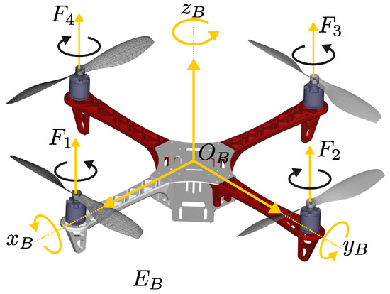
Figure 1.
Multicopter forces.
The multicopter dynamic model can be derived using the Newton–Euler formalism in the body fixed frame , about the multicopter subject to external forces and moments applied to the center of mass. Thus, the dynamic equations of motion are described by:
where is the translational velocity of the airframe, is the angular velocity of the aircraft, is the inertia tensor, and m is the mass. The force and torque are produced by propeller system, and are the aerodynamic forces and moments vectors which act on the multicopter by blade flapping, is the gyroscopic moment effect produced by the change in orientation of the rotor-craft, and is the gravity effect forces vector with m/s2. These variables are defined as:
where d is the distance from the center of mass to the rotor shaft, c is the drag factor, is the rotor inertia, is the speed of the rotor i, is the aerodynamic function with , where the air density, is the aerodynamic coefficient, and is the element of , which is the velocity of the multicopter with respect to the air [30].
4. Control
The control objective is to track a three-dimensional reference, , as well as the yaw angle reference, , with known derivatives. Adaptive backstepping [31], nonlinear– [32], and Sliding–Mode techniques [33] are combined to ensure trajectory tracking.
The models (7) and (8) are presented in a block state space as:
where the variables are replaced as follows:
Also, is the speed of the rotor i, is the aerodynamic acceleration expressed in the inertia reference frame , and is the equivalent rotational acceleration, that is, the acceleration computed from the aerodynamic functions and , respectively. Let us define the outputs as , where , , and
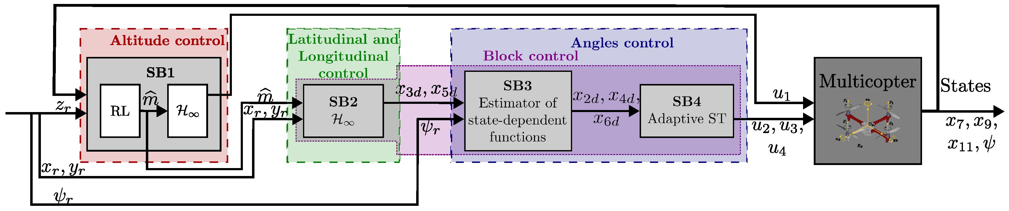
Hereafter, tracking is designed for altitude () with subblock through input , subsequently, for longitude () and latitude () control with subblock using the variables and , which are manipulated along with to track through , , and with subblocks and . Figure 2 shows the details of the proposed control.
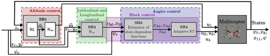
Figure 2.
Diagram of the proposed controller scheme.
4.1. Altitude Control
Define the tracking error as follows:
where is the reference signal. Then, using (9), the tracking error dynamics are obtained as:
The control in (14) is formulated as:
where is the vector error of altitude tracking and the gain is chosen to achieve the nominal system be stable. In addition, will be designed to reject the unknown perturbation. The mass estimation is calculated from Reinforcement Learning, as in [34], using state estimator:
where is the state estimation error. Hence, the adaptive law for the estimation of mass is:
with a positive scalar .
The system (17) can be represented in the matrix form as:
where
and the pair is assumed to be observable.
The robust control part is formulated using the -control technique [35,36,37], as follows:
where is a positive definite matrix solution of Riccati equation:
where and are some positive constants.
As result, the response , for initial state , satisfies:
where .
Moreover, according to the work of Arellano-Muro et al. [34], the adaptation error is bounded by:
for some and a constant .
To show the stability of the closed-loop subsystem (18) with (16), para y , define a Lyapunov function:
Taking the time derivative of the Lyapunov function and using (18) results in:
Suppose that, in the equilibrium point of the closed-loop subsystem , the perturbation term holds under the limits:
where and are real positive constants in some admissible region .
Setting from (20), results in:
Choosing:
the norm is ultimately bounded in an admissible region , that is:
where for all .
As a result, the following proposition is enunciated: the closed-loop solution (18) using the adaptive law (16) is asymptotically stable in an admissible region and the adaptive error is bounded for .
Since stays on the ball , so does the tracking error and the mass estimate since the error is also bounded.
4.2. Latitudinal, Longitudinal, and Yaw Control
Considering the subsystem (10), define the tracking error vector as:
where and are the references signals. Then, the tracking error dynamics are obtained as:
Considering the vector as a virtual control in (22), we choose its desired value as:
with
and is formulated using -control to attenuate the disturbance and of the closed-loop subsystem (21) and (23), where the vector is defined as:
where
so that we can establish , where is a symmetric positive definite matrix solution of Riccati equation:
with sufficiently small constant and some positive constant .
Define now the following:
where is calculated as a recursive solution to the following expression:
as a function of the given reference for the system output and the desired values and .
Calculating the derivative as:
the system (27) becomes:
where the following matrix:
is considered as known, while the following matrix:
and the vector
are considered unknown.
The following assumption is instrumental to get the desired result.
Assumption 1.
The unknown vector and matrix are bounded, and they can be expressed as a Kronecker series:
where and are defined. Moreover, with and the operator is a Kronecker product. We have and as constants.
Defining as an estimate of with the following dynamics:
where
with N any positive constant, also:
where is the adaptation error and and are constants to be adapted with the law:
Using (30) and (31) with (29) and (32), the estimation error dynamics become:
where and are the adaptation errors, , and are the parameters errors, and the term is considered a bounded disturbance:
On the next step of the design procedure, considering the variables , , and in (28) as the virtual controls, its desired values are chosen of the form:
Defining the control error:
and using the subsystem (12) yields
where
Defining as the estimate of the parameter , the control is formulated as:
where is a symmetric positive definite matrix and is a diagonal matrix. The adaptation law is proposed of the form:
The following assumption will be used to analyze stability of the system (40) and (41).
Assumption 2.
Additionally, from Assumption 1, it follows that is also bounded, and thus:
To demonstrate the stability of the closed-loop system (40), (41) note input-to-state stability in (40) with and as input and asymptotic stability of system (41). Along with [38], let us consider the first Lyapunov function candidate to unforced system (40):
choosing a constant , from (25), we obtain:
Thus, the solution is exponentially tends to zero. Now, consider the second Lyapunov function candidate:
where and is a positive constant.
Calculating its time derivative along the trajectories of the system (41) yields:
Let us introduce a positive constant , and assign , to obtain:
where
for a neighbor close to , such that , this is:
Thus, the Lyapunov function derivative is negative semi-definite. Through Barbalat’s lemma and LaSalle’s invariance principle, it is easy to see that the solution tends asymptotically to zero, and the parameter estimates are bounded.
Finally, choosing the Lyapunov function of cascade system (40) and (41) as [39], whose derivative is represented in (42) and (45), yields:
Replacing the bounds of the disturbances results in:
choosing
where
Thus, the Lyapunov function is negative semi-definite for all:
however, a solution is ultimately bounded as follows [40]:
Thus, the tracking error , from (21), is also ultimately bounded. However, since the solution tends asymptotically to zero then, the output tends to asymptotically.
5. Simulation Results
To demonstrate the effectiveness of the proposed control scheme, a hypothetical scenario is presented in which an aircraft with an initially unknown load travels through four points to unload part of it. For simulation purposes, a sequence of checkpoints i (), where are chosen as , , , , and meters at intervals of 4 s; each checkpoint is a set of reference . In the mass is released, and Table 1 shows the loads to be released.

Table 1.
Loads to be released at each checkpoint.
The parameters used are shown in Table 2. During the simulation, the inertias are modified with respect to the relation of the total and nominal mass.
Table 2.
Parameters of quadrotor.
For the altitude block in control law (15), is defined, and for the adaptive dynamics (16), is established. The gain of the part is to find resolving (19) con y , resulting in:
Likewise, for the latitudinal–longitudinal block , the gain control (23) is established as . The matrix gain for the part that attenuates the unmatched disturbances is to be found through (25):
using and .
Finally, the gains in (37), are as follows: and .
To prove control robustness, the velocity wind in aerodynamic functions [30], is set in time dependence as:
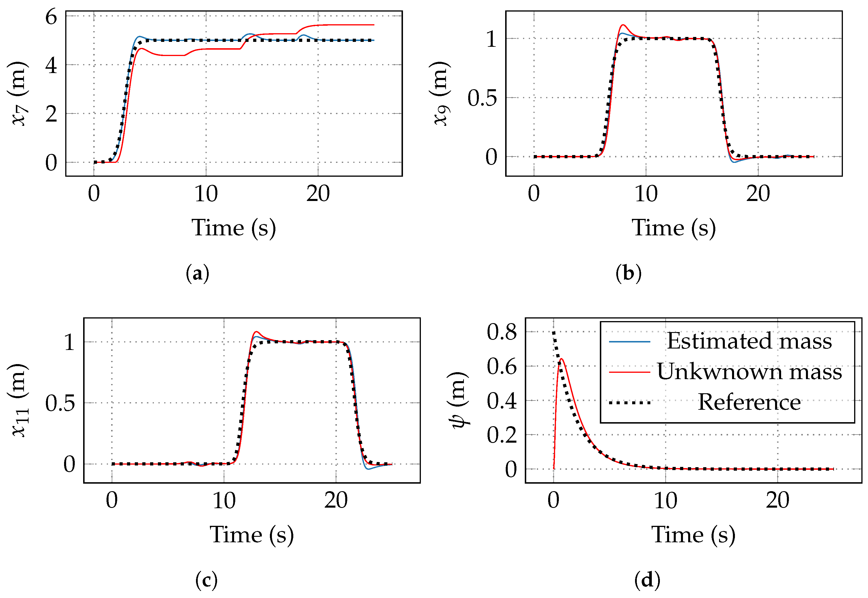
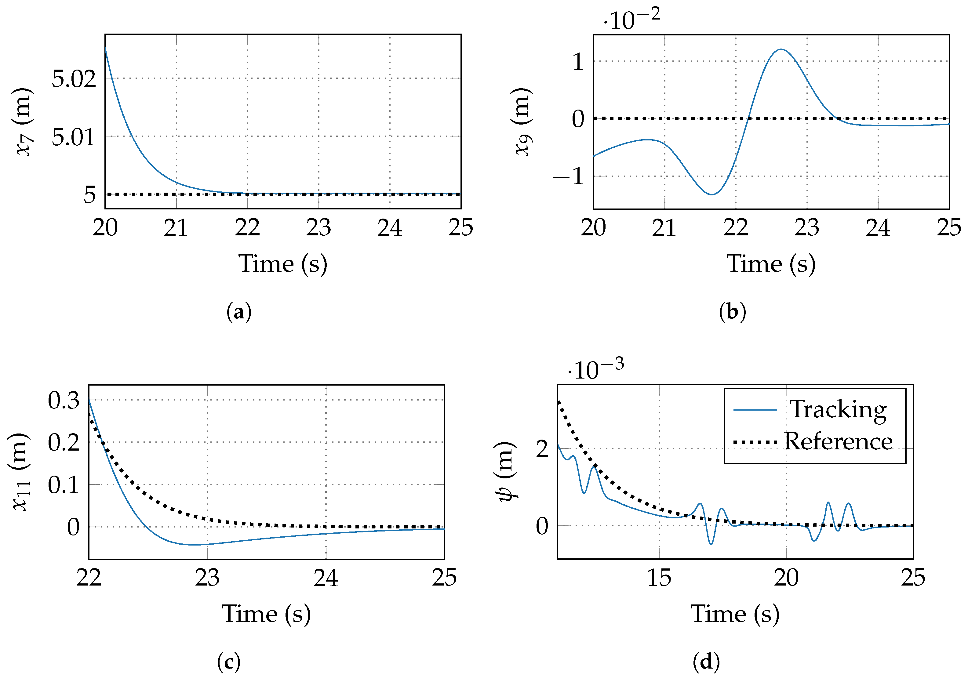
In the graphs of Figure 3, tracking using the proposed adaptive control scheme (blue line) is seen. Another one (red line) is also shown, with the control without adapting the parameters, that is, setting Equations (16) and (38) as zero at all times. Figure 3a–d are depicted the tracking of positions z, x, y, and orientation, respectively. The tracking in the Earth reference frame is shown in Figure 4. Notice that the chattering is not significant due to the ST action. Figure 5 shows the detail at , when all the surfaces are zero in the ST algorithm.
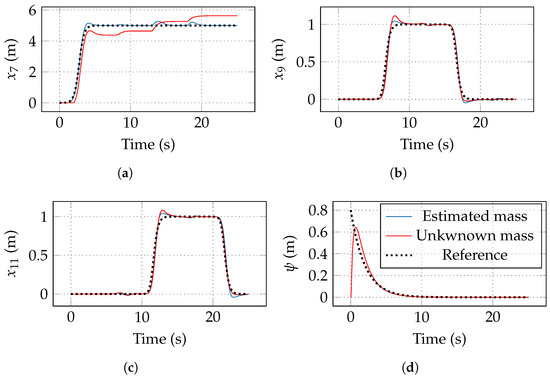
Figure 3.
Control tracking comparison between robust (red) and adaptive–robust control (blue) of the output vector. (a) Tracking of z altitude. (b) Tracking of x longitude. (c) Tracking of y latitude. (d) Tracking of yaw.
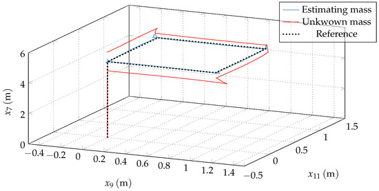
Figure 4.
Tracking of the 3D space in the Earth reference frame.

Figure 5.
Zoom in of to see the detail of low chattering. (a) Zoom in of the tracking of z altitude. (b) Zoom in of the tracking of x longitude. (c) Zoom in of the tracking of y latitude. (d) Zoom in of the tracking of yaw.
Estimation of the total mass using the Discontinuous Gradient algorithm is shown in Figure 6. In the first 8 s, the mass is the sum of all the loads and the nominal one, that is ; then, in , the resulting mass is the sum of all of them when is released, that is . Afterward, at time , the load of mass is released, and hence, the total mass is ; finally, when the quadrotor arrives to , at time , the mass is discharged, where the total mass equals m until the end of simulation. On the other hand, chattering in mass adaptation is not noticeable, thanks to the integral action in the finite-time mass estimation algorithm.
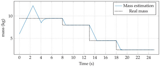
Figure 6.
Mass estimation using the Discontinuous Gradient algorithm.
6. Conclusions
This paper presents a model-based nonlinear controller for quadrotors aerial vehicles in which the plant model is given in terms of quaternions reducing the computational cost of executing model-based control laws. The study is developed for a scenario in which mass variations and external wind perturbations cannot be neglected, and a Super-Twisting Sliding-Mode control strategy combination ensures that the trajectory tracking control task is performed even in the presence of external perturbation and system mass variations. Simulation results, obtained with MATLAB R2023a/Simulink, show that the accuracy of the proposed control approach, in terms of trajectory tracking error, is higher if compared with other control strategies that do not consider parameter variations. To compare the quality and performance of the proposed approach concerning existing control methods, in future works, the use of a disturbance observer along with a finite-time parameter estimator will be explored.
Author Contributions
Methodology, C.A.A.-M.; software, C.A.A.-M.; formal analysis, C.A.A.-M.; investigation, R.C.; resources, R.C.; visualization, G.L.O.-G.; funding acquisition, R.C. All authors have read and agreed to the published version of the manuscript.
Funding
This research received no external funding.
Data Availability Statement
The original contributions presented in the study are included in the article, further inquiries can be directed to the corresponding author.
Conflicts of Interest
The authors declare no conflicts of interest.
References
- Silva, L.A.; Leithardt, V.R.Q.; Batista, V.F.L.; Villarrubia González, G.; De Paz Santana, J.F. Automated Road Damage Detection Using UAV Images and Deep Learning Techniques. IEEE Access 2023, 11, 62918–62931. [Google Scholar] [CrossRef]
- Sun, Y.; Shao, Z.; Cheng, G.; Huang, X.; Wang, Z. Road and Car Extraction Using UAV Images via Efficient Dual Contextual Parsing Network. IEEE Trans. Geosci. Remote Sens. 2022, 60, 1–13. [Google Scholar] [CrossRef]
- Cheng, L.; Zhong, L.; Tian, S.; Xing, J. Task Assignment Algorithm for Road Patrol by Multiple UAVs With Multiple Bases and Rechargeable Endurance. IEEE Access 2019, 7, 144381–144397. [Google Scholar] [CrossRef]
- Pan, Y.; Zhang, X.; Cervone, G.; Yang, L. Detection of Asphalt Pavement Potholes and Cracks Based on the Unmanned Aerial Vehicle Multispectral Imagery. IEEE J. Sel. Top. Appl. Earth Obs. Remote Sens. 2018, 11, 3701–3712. [Google Scholar] [CrossRef]
- Sun, Y.; Abeywickrama, S.; Jayasinghe, L.; Yuen, C.; Chen, J.; Zhang, M. Micro-Doppler Signature-Based Detection, Classification, and Localization of Small UAV With Long Short-Term Memory Neural Network. IEEE Trans. Geosci. Remote Sens. 2021, 59, 6285–6300. [Google Scholar] [CrossRef]
- Shakhatreh, H.; Sawalmeh, A.H.; Al-Fuqaha, A.; Dou, Z.; Almaita, E.; Khalil, I.; Othman, N.S.; Khreishah, A.; Guizani, M. Unmanned Aerial Vehicles (UAVs): A Survey on Civil Applications and Key Research Challenges. IEEE Access 2019, 7, 48572–48634. [Google Scholar] [CrossRef]
- Khosravi, M.R.; Samadi, S. Mobile multimedia computing in cyber-physical surveillance services through UAV-borne Video-SAR: A taxonomy of intelligent data processing for IoMT-enabled radar sensor networks. Tsinghua Sci. Technol. 2022, 27, 288–302. [Google Scholar] [CrossRef]
- Shao, Z.; Cheng, G.; Ma, J.; Wang, Z.; Wang, J.; Li, D. Real-Time and Accurate UAV Pedestrian Detection for Social Distancing Monitoring in COVID-19 Pandemic. IEEE Trans. Multimed. 2022, 24, 2069–2083. [Google Scholar] [CrossRef]
- Yang, L.; Fan, J.; Liu, Y.; Li, E.; Peng, J.; Liang, Z. A Review on State-of-the-Art Power Line Inspection Techniques. IEEE Trans. Instrum. Meas. 2020, 69, 9350–9365. [Google Scholar] [CrossRef]
- Quater, P.B.; Grimaccia, F.; Leva, S.; Mussetta, M.; Aghaei, M. Light Unmanned Aerial Vehicles (UAVs) for Cooperative Inspection of PV Plants. IEEE J. Photovolt. 2014, 4, 1107–1113. [Google Scholar] [CrossRef]
- Sadykova, D.; Pernebayeva, D.; Bagheri, M.; James, A. IN-YOLO: Real-Time Detection of Outdoor High Voltage Insulators Using UAV Imaging. IEEE Trans. Power Deliv. 2020, 35, 1599–1601. [Google Scholar] [CrossRef]
- Tang, S.; Wüest, V.; Kumar, V. Aggressive Flight With Suspended Payloads Using Vision-Based Control. IEEE Robot. Autom. Lett. 2018, 3, 1152–1159. [Google Scholar] [CrossRef]
- Xian, B.; Wang, S.; Yang, S. An Online Trajectory Planning Approach for a Quadrotor UAV With a Slung Payload. IEEE Trans. Ind. Electron. 2020, 67, 6669–6678. [Google Scholar] [CrossRef]
- Du, Z.H.; Wu, H.N.; Feng, S. Boundary Control of a Quadrotor UAV with a Payload Connected by a Flexible Cable. In Proceedings of the 2018 37th Chinese Control Conference (CCC), Wuhan, China, 25–27 July 2018; pp. 1151–1156. [Google Scholar] [CrossRef]
- Pereira, P.O.; Dimarogonas, D.V. Control framework for slung load transportation with two aerial vehicles. In Proceedings of the 2017 IEEE 56th Annual Conference on Decision and Control (CDC), Melbourne, Australia, 12–15 December 2017; pp. 4254–4259. [Google Scholar] [CrossRef]
- Ariyibi, S.; Tekinalp, O. Control of a Quadrotor Formation Carrying a Slung Load Using Flexible Bars. In Proceedings of the AIAA Aviation 2019 Forum, Dallas, TX, USA, 17–21 June 2019. [Google Scholar] [CrossRef]
- Yu, G.; Cabecinhas, D.; Cunha, R.; Silvestre, C. Nonlinear Backstepping Control of a Quadrotor-Slung Load System. IEEE/ASME Trans. Mechatron. 2019, 24, 2304–2315. [Google Scholar] [CrossRef]
- Wu, C.; Fu, Z.; Yang, J.; Wei, Y. Nonlinear control and analysis of a quadrotor with sling load in path tracking. In Proceedings of the 2017 36th Chinese Control Conference (CCC), Dalian, China, 26–28 July 2017; pp. 6519–6524. [Google Scholar] [CrossRef]
- BBVA.Drones: Los Aliados de la Agricultura de Precisión y la Industria Alimentaria. 2023. Available online: https://www.bbva.com/es/sostenibilidad/drones-los-aliados-de-la-agricultura-de-precision-y-la-industria-alimentaria/ (accessed on 12 September 2024).
- IWATA. Yamaha Motor Signs to Collaborate with Australian AgTech Company, the Yield, for Smart Agricultural Solutions—Toward Labor Saving, Efficiency Improvements, and Optimization through Partnerships with Agricultural Startups. 2021. Available online: https://global.yamaha-motor.com/news/2021/0609/corporate.html (accessed on 12 September 2024).
- Staff Amazon. Amazon Announces 8 Innovations to Better Deliver for Customers, Support Employees, and Give Back to Communities Around the World. 2023. Available online: https://www.aboutamazon.com/news/operations/amazon-delivering-the-future-2023-announcements (accessed on 12 September 2024).
- Stephan, F.; Reinsperger, N.; Grünthal, M.; Paulicke, D.; Jahn, P. Human drone interaction in delivery of medical supplies: A scoping review of experimental studies. PLoS ONE 2022, 17, e0267664. [Google Scholar] [CrossRef]
- Al-Rawashdeh, Y.M.; Elshafei, M.; Ouakad, H.M. In-flight estimation of quadrotor mass and inertia using all-accelerometer. J. Vib. Control 2023, 30, 3034–3047. [Google Scholar] [CrossRef]
- Wong, T.L.; Khan, R.R.; Lee, D. Model Linearization and H∞ Controller Design for a Quadrotor Unmanned Air Vehicle: Simulation Study. In Proceedings of the 13th International Conference on Control, Automation, Robotics and Vision, Singapore, 10–12 December 2014. [Google Scholar]
- Arellano-Muro, C.A.; Luque-Vega, L.F.; Castillo-Toledo, B.; Loukianov, A.G. Backstepping Control with Sliding Mode Estimaton for a Hexacopter. In Proceedings of the 10th International Conference on Electrical Engineering, Computing Science and Automatic Control (CCE), Mexico City, Mexico, 30 September–4 October 2013. [Google Scholar]
- Benallegue, A.; Mokhtari, A.; Fridman, L. Feedback linearization and high order sliding mode observer for a quadrotor UAV. In Proceedings of the Variable Structure Systems, VSS’06, International Workshop on IEEE, Alghero, Italy, 5–7 June 2006; pp. 365–372. [Google Scholar]
- Siciliano, B.; Sciavicco, L.; Luigi Villani, G.O. Robotics Modelling, Planing and Control; Springer: London, UK, 2009. [Google Scholar]
- Arellano-Muro, C.A.; Castillo-Toledo, B.; Loukianov, A.; Luque-Vega, L.F.; Gonzalez-Jimenez, L. Quaternion-based Trajectory Tracking Robust Control for a Quadrotor. In Proceedings of the 10th Annual System of Systems Engineering Conference 2015 (SoSE 2015), San Antonio, TX, USA, 17–20 May 2015. [Google Scholar]
- Alaimo, A.; Artale, V.; Milazzo, C.; Ricciadello, A.; Trefiletti, L. Mathematical Modeling and Control of a Hexacopter. In Proceedings of the International Conference on Unmanned Aircraft Systems (ICUAS), Atlanta, GA, USA, 28–31 May 2013. [Google Scholar]
- Gessow, A.; Myers, G.C. Aerodynamics of the Helicopter, 5th ed.; Frederick Unger Publishing Co.: New York, NY, USA, 1978. [Google Scholar]
- Marino, R.; Tomei, P. Nonlinear Control Design. Geometric, Adaptive and Robust; Prentice Hall: Saddle River, NJ, USA, 1995. [Google Scholar]
- Isidori, A.; Astolfi, A. Disturbance Attenuation and H∞-Control Via Measurement Feedback in Nonlinear Svstems. IEEE Trans. Autom. Control 1992, 1283–1293. [Google Scholar] [CrossRef]
- Levant, A. Universal single-input–single-output (SISO) sliding-mode controllers with finite time convergence. IEEE Trans. Autom. Control 2005, 46, 1785–1789. [Google Scholar] [CrossRef]
- Arellano-Muro, C.A.; Castillo-Toledo, B.; Di Gennaro, S.; Loukianov, A.G. Online Reinforcement Learning Control via Discontinuous Gradient. Int. J. Adapt. Control Signal Process. 2024, 38, 1762–1776. [Google Scholar] [CrossRef]
- Aguilar, L.; Orlov, Y.; Acho, L. Nonlinear H∞-control of nonsmooth time-varying systems with application to mechanical manipulators. Automatica 2003, 39, 1531–1542. [Google Scholar] [CrossRef]
- Loukianov, A.G.; Rivera, J.; Orlov, Y.V.; Teraoka, E.Y.M. Robust Trajectory Tracking for an Electrohydraulic Actuator. IEEE Trans. Ind. Electron. 2009, 56, 3523–3531. [Google Scholar] [CrossRef]
- Aliyu, M. Nonlinear-Control, Hamiltonian Systems and Hamilton–Jacobi Equations; CRC Press: Boca Raton, FL, USA, 2011. [Google Scholar]
- Mahapatro, S.R.; Subudhi, B.; Ghosh, S. Design and real-time implementation of an adaptive fuzzy sliding mode controller for a coupled tank system. Int. J. Numer. Model. Electron. Netw. Devices Fields 2019, 32, e2485. [Google Scholar] [CrossRef]
- Sontag, E.; Teel, A. Changing supply functions in input/state stable systems. IEEE Trans. Autom. Control 1995, 40, 1476–1478. [Google Scholar] [CrossRef]
- Khalil, H.K. Nonlinear Systems; Prentice Hall: Saddle River, NJ, USA, 2002. [Google Scholar]


Disclaimer/Publisher’s Note: The statements, opinions and data contained in all publications are solely those of the individual author(s) and contributor(s) and not of MDPI and/or the editor(s). MDPI and/or the editor(s) disclaim responsibility for any injury to people or property resulting from any ideas, methods, instructions or products referred to in the content. |
© 2024 by the authors. Licensee MDPI, Basel, Switzerland. This article is an open access article distributed under the terms and conditions of the Creative Commons Attribution (CC BY) license (https://creativecommons.org/licenses/by/4.0/).