Abstract
This paper compares two statistical methods for parameter reconstruction (random drift and diffusion coefficients of the Itô stochastic differential equation, SDE) in the problem of stochastic modeling of air–sea heat flux increment evolution. The first method relates to a nonparametric estimation of the transition probabilities (wherein consistency is proven). The second approach is a semiparametric reconstruction based on the approximation of the SDE solution (in terms of distributions) by finite normal mixtures using the maximum likelihood estimates of the unknown parameters. This approach does not require any additional assumptions for the coefficients, with the exception of those guaranteeing the existence of the solution to the SDE itself. It is demonstrated that the corresponding conditions hold for the analyzed data. The comparison is carried out on the simulated samples, modeling the case where the SDE random coefficients are represented in trigonometric form, which is related to common climatic models, as well as on the ERA5 reanalysis data of the sensible and latent heat fluxes in the North Atlantic for 1979–2022. It is shown that the results of these two methods are close to each other in a quantitative sense, but differ somewhat in temporal variability and spatial localization. The differences during the observed period are analyzed, and their geophysical interpretations are presented. The semiparametric approach seems promising for physics-informed machine learning models.
Keywords:
stochastic model; stochastic differential equation; parametric estimation; nonparametric estimation; semiparametric approach; finite normal mixtures; EM algorithm; heat fluxes; air–sea interaction; North Atlantic MSC:
65C30; 60H30; 86-04; 86-08; 86-10
1. Introduction
In the ocean–atmosphere system, the heat flux behavior and each component’s variability play important roles, as they have significant impacts [1] on the climatic features of this system, making their quantitative and qualitative analysis one of the main problems in modern oceanology and climatology. The distribution of the sensible and latent heat fluxes was previously examined and approximated using the two-parameter Fisher–Tippett distribution.
In this paper, the well-known Itô stochastic differential equation (SDE) [2] is used as the model of the dynamics of heat flux variability in the air–sea system. The problem of estimating the (generally speaking) random coefficients of the SDE, given the observations of the process, implies some significant assumptions on the mathematical properties of coefficients [3,4,5,6]. In papers [3,4,5,6], the authors suppose the coefficients to be functions of the unknown parameter ; some of them even assume a specific type of dependence on the parameter. In paper [7], the nonparametric case is considered, and the estimate of the diffusion coefficient, along with proving its convergence and consistency, is obtained under the assumption of existence of the three continuous bounded derivatives of this coefficient and non-randomness and existence of bounded derivatives of the drift coefficient. A kernel-based regression method [8] can also be used.
The application of the Itô model for heat flux increment evolution was previously studied in paper [9]. The Itô SDE model generalizes the well-known statistical models of climate dynamics, in particular, those by Budyko [10] and Hasselmann [11]. This model also appears in [12,13], where the authors used it to describe the behavior of the heat fluxes between ice and the ocean in the Arctic region. The model’s statistical features in the two-dimensional case were thoroughly examined in [2]. The estimation of the unknown model parameter in the multidimensional case of the Langevin equation, which is variant for the Itô equation, was proposed in [14].
The drift parameter of the Itô equation corresponds to the mean changes in the behavior of the system over time, depending both on a particular moment in time and on the value of the flux. The identification of the areas where this coefficient is significant can be useful to determine the zones of jet streams, fronts, and synoptic vortices, where significant dynamic processes occur. The areas with a small drift coefficient and a large stochastic (diffusion) coefficient correspond to areas of strong turbulence, including energy-active areas in the North Atlantic. Therefore, the task of estimating the parameters of the stochastic model of heat fluxes’ increment behavior is important for solving the problems from the mathematical modeling point of view.
The modeling of the increments of the fluxes (in contrast to the traditionally used one for studying the values of the fluxes themselves) adequately describes the dynamics of fluxes in the medium and long term and appears to be in good agreement with the real data. This model has a few advantages over the known numerical or stochastic ones. It is quite simple, since the form of the model is determined with two coefficients, even in the multidimensional case (the drift vector and the diffusion matrix). Thereby, it is possible to quantitatively estimate the behavior of the studied characteristics, i.e., to analyze and forecast them. Additionally, this scheme is quite general, since it includes both the dynamic models with random forcing (i.e., an external influence), as well as the models that are based on trends in the periodic and random components. To test the adequacy of the model, the authors previously considered the statistical regularities of the intra- and interannual variability in the sensible and latent heat fluxes in the North Atlantic by using the time series from the ERA5 reanalysis database [15]. The behavior of the maximums, minimums, means, and medians over the considered water area over time was studied. It was shown that there is a positive trend in the latent heat flux dynamics, and its parameters were estimated. The proposed model uses the well-developed apparatus of the theory of stochastic differential equations and parabolic Fokker–Planck–Kolmogorov equations; therefore, it is convenient for quantitative and qualitative assessments of the fluxes’ dynamics, their spatiotemporal variability, and the probabilities of occurrence of rare but dangerous events—for example, tropical hurricanes.
As was noted above, the nonparametric method has rigorous theoretical substantiations; however, it requires the fulfillment of some set of conditions for the coefficients that often cannot be verified for real geophysical data. The alternative considered approach is the semiparametric statistical method, based on reconstructing the distributions of the unknown random drift and diffusion coefficients of SDE, which implies that the estimation process is carried out using a set of arbitrary shift-scale normal mixtures. It is worth noting that, in the case of the non-random coefficients of the considered SDE, when making additional assumptions about measurability with respect to natural filtering and normality of the distribution of the initial process value, the solution appears to be some Gaussian process with a given mean and covariance function. A strict theoretical formulation of the convergence problem for the semiparametric method is complicated; this issue is discussed below in this paper (see Section 3.3). Therefore, in this article, the semiparametric approach, which is free from any additional assumptions, is compared with a nonparametric one to demonstrate the proximity of the results and, as a consequence, the correctness of its application. One of the important potential applications of the semiparametric method relates to the forecasting problem. Within it, theoretically justified approximations of the distributions for the SDE solutions arise. These distributions, or, rather, the parameters and the connectivity components obtained from their estimation, could be used within the framework of physics-informed machine learning (ML). Some examples of effective improvement of neural network forecasts using this method were demonstrated earlier in [16] for a few heat fluxes in the Labrador Sea and the Gulf Stream. It is worth noting that obtaining the point estimates by the first approach, in this case, may require solving multiple SDEs.
To test and compare the accuracy of the two methods, an implementation of a random process with given coefficients in the form of a linear combination of trigonometric functions is generated. In addition, a quantitative comparison of the proposed methods is carried out on the latent and sensible heat fluxes in the North Atlantic using the reanalysis data from the ERA5 database for the 1979–2022 period. It is shown that the results of both methods are quite close. For the cases of some difference in the results, geophysical interpretation is suggested.
The main contributions of this paper are as follows:
- The realization of the semiparametric approach for reconstructing the dynamic-stochastic model’s parameters, with the possibility of their further usage for solving forecasting problems by some physics-informed machine learning methods;
- The comparison of the semiparametric (not requiring any additional assumptions on the data) results with the estimates obtained by the nonparametric method (for which the theoretical properties, such as the consistency of the estimates, are known) on the simulated data;
- The comparison of the approaches by applying them to the reanalysis data of the latent and sensible heat fluxes from the ERA5 database for the 1979–2022 period, and the geophysical interpretation of the differences in the obtained results for the real spatiotemporal data.
The rest of the paper is organized as follows. Section 2 presents the mathematical model based on the Itô equations, as well as the demonstration of the SDE solution existence for the reanalysis data. Section 3 contains the description of the two approaches for reconstructing the random coefficients of the SDE: the nonparametric one, which uses frequency estimation, and the semiparametric one, based on finite normal mixtures. It also compares both methods by using simulated trigonometric data, which are related to the common climatic models. Section 4 concerns the comparison of the results of both methods applied to the reanalysis data in the North Atlantic for the 1979–2022 period. Section 5 summarizes the obtained results from the geophysical point of view and discusses possible directions for further research, including forecasting problems.
2. Problem Statement
In this research, a stochastic differential equation of the form
is used as a mathematical model of the heat flux increments. The SDE is called the Itô equation, where is a random process whose values at a fixed time moment have the meaning of a vector of sensible and latent heat flux values. and are the drift and diffusion coefficients, whose values depend on the time and the corresponding flux value and are random variables. is a standard Wiener process that is independent of . The initial value is supposed to be known and independent of all differences . However, its exact value is not required, since Equation (1) corresponds to the increments of the process.
Further, a discrete random process at the time moments , with its values known in the nodes of the grid forming the matrix of size , is considered, that is,
The corresponding random coefficients from the Itô equation that depend on the value of the flux appear as matrices of the corresponding size:
In this paper, both synthetically generated data and the real data of the evolution of sensible and latent heat fluxes from the ERA5 reanalysis database are used to check the quality of the methods’ estimates. The flux values of the reanalysis data are given in the nodes of a uniform one-degree grid of 161 × 181 points, corresponding to the geographic area of the North Atlantic Ocean and covering latitudes from 0° to 80° and longitudes from −90° to 0° during the period from January 1979 to December 2022. The four measurements per day are taken with a six-hour step: at 00:00, 06:00, 12:00, and 18:00. When constructing the estimates, a time step of one day between consecutive measurements was considered. Therefore, before applying these methods, the data were previously grouped by four consecutive values and averaged in order to obtain the mean daily value of the flux. It can be demonstrated that the conditions of the SDE solution’s existence are satisfied for these data (see book [17], page 469).
The solution of the SDE in (1) is a diffusion process with diffusion coefficient and drift coefficient . The random coefficients and are the conditional expectation and the variance of the flux increments, respectively:
where and are expectation and variance of the random variable, respectively.
Assume that and are Borel functions, defined for . Then, the considered SDE is equivalent to the following equation (the initial condition is assumed to be given):
For the existence of a solution to the Equation (1) for some , the following conditions [17] are to be satisfied:
Moreover, if and are two continuous solutions for a fixed , then they are indistinguishable.
To check the conditions in (2) and (3) for the analyzed data, an estimate for the constant is constructed. Considering the case for the first inequality, the constant has the following form:
For the inequality in (3), taking into account that , it follows that
There is a small number of outliers in the data, which can have values several times larger than the typical values of the coefficients. To determine the coefficients in the inequalities, they were excluded: a quantile on the order of was chosen as the maximum for each type of flux, and was the minimum.
Due to the volume of data, it is difficult to calculate the quantiles over the entire time interval at the same time, so the quantiles were calculated several times over the data from consecutive days. Then, the maximum was taken as the upper quantile, and the minimum was taken as the lower quantile. In addition, a non-zero separability of the difference from is assumed, empirically choosing that the threshold equals .
Taking into account the introduced restrictions, the following values of the upper and lower quantiles for and were obtained: (from the physical sense, the cases of complex and, therefore, negative values are not considered), . Thus, the following estimates of the constants were obtained: for the inequality in (2) and, for the inequality in (3), . Thus, the finite value of exists, guaranteeing the correctness of applying the mathematical model used in the paper to the considered heat flux data.
It is worth noting that this proof can be extended for the two-dimensional case, which will be considered in our next papers.
3. Methodology of Reconstruction
In the absence of a priori information about the “physical” structure of the process , the problem of statistical reconstruction of the functions and becomes the one of the utmost importance. Due to their randomness, this task allows at least two fundamentally different approaches for its formulation. The first one is to obtain the estimates (which would be random themselves) of the and functions, that is, to construct their point approximations (see Section 3.2). The second approach represents the statistical reconstruction of random coefficients and in terms of their distributions. That is, knowing some properties of these coefficients, one can find the estimates of some numerical parameters of these models. Both approaches can be interpreted as physically realistic and feasible ones.
3.1. Data Discretization
The implementation of the computational procedures requires data preprocessing, within which the flux values, which can be any real numbers, are replaced by the nearest fixed value from some fixed intervals, that is, the process values are actually discretized in space. That is, for a certain period of time, all values of the process are sorted in ascending order, and a significant number of quantiles of different levels, uniformly covering the segment are picked out. This is necessary to select a set of intervals for which the probabilities of a new observation falling into each particular interval would be as close to each other as possible.
Then, a procedure similar to rounding numbers is carried out. For each set of grid nodes, in which the process values fall into the interval between the two consecutive quantiles with numbers and , the values are replaced by the half-sum of these two quantiles, and this operation is carried for all That is, each value is “rounded” to the nearest number from the set of half-sums of neighboring quantiles. Thus, after this transformation, at each grid point, there can be only one of the possible fixed values. The resulting process with possible states, corresponding to the original one , is denoted as .
3.2. Nonparametric Estimation
This method was proposed in the work [9] and is based on the assumption that all statistical characteristics of the quantities under consideration depend only on the values themselves and do not depend on their geographical coordinates. In other words, this assumption means that the values of the process, taken at different points in space, belong to the same general population with certain statistical characteristics. For the heat fluxes between the ocean and the atmosphere, this assumption appears to be quite reasonable, since the traditional calculation formulas for the fluxes (see, for example, [18,19]) use only the values of the contact media themselves, but not their location.
The first step of this method is the transformation of the set of all available values of the flux increments for the considered time interval at all grid nodes to a significantly smaller set of values, using the discretization procedure described earlier. For example, for the real fluxes data in the nodes of the grid with size , for a time interval of years (with one value per day), the cardinality of the set of states, to which all initial values were reduced, was chosen to be equal to .
Further, for each pair of successive time moments and , the corresponding matrices with values of the discrete process are considered, denoting them as and . For each of the possible values of the process at time moment and at time moment , the transition probability for this pair of states is estimated by the ratio of the number of matrix points having the value at time and the value at time to the number of points having the value at the time :
where the symbol # denotes the number of elements that satisfy the conditions specified in brackets. If, for some pair, it holds that , the corresponding probability is set to zero.
As such, each pair of successive time moments and correspond to the transition matrix with size , which is henceforth used to construct the desired estimates for random coefficients and The notation is further used for denoting the matrix of the coefficient estimates at time moment with a size of . For a fixed value at the nodes, for which , only that is chosen, which is present at least at one point of the matrix. This set of coordinates is further denoted as where the number of nodes can generally take any value from the range . Further, for the previously fixed value at the points with coordinates , the coefficient estimates matrix is set equal to
To construct the whole matrix of estimates , it is necessary to perform this operation for all possible values .
Similarly, for the square of the coefficient , the estimation matrix at points with coordinates is set equal to
To obtain the estimates of the random coefficient itself, a square root from the values of the estimation matrix is taken.
The consistency of such non-parametric estimates can be theoretically proven. Indeed, the frequency estimations for the transition matrices are well-known and consistent. That means that, if the length of the sample is large enough, the frequency converges to the sought transitional probability with respect to the probability distribution. Hence, the estimations of the random coefficients and will also converge with respect to the probability. The next step is to show that, if the distance between two consecutive time moments approaches zero, then the Markov chain converges to the diffusion stochastic process. This has been proven in [20]. Finally, since the stochastic equations considered in this paper have a unique solution, the converged statistics will estimate the necessary parameters. This completes the proof of the consistency of the constrained nonparametric statistics.
3.3. Semiparametric Reconstruction
It is known [21] that, for an Itô SDE (1) with nonrandom coefficients, under additional assumptions about the measurability of the process with respect to the natural filtration and the normality of the distribution of the initial value, the solution has the form of some Gaussian process with a given mean and covariance function. In this situation, the process increments are also Gaussian random variables. However, if each parameter is random, the distributions of the form , that is, shift-scale normal mixtures, arise naturally. It is more appropriate to speak of a reconstruction of the coefficients of the stochastic differential equation rather than of their estimation. The suggested semiparametric approach makes it possible to reconstruct the joint one-dimensional distributions of the drift and diffusion coefficients. For this purpose, a part of the original time series (the window) is chosen and the observations in this window are considered as a homogeneous sample. The theoretical distribution of these observations are shift-scale normal mixture. For the mathematical correctness of the problem, the continuous normal mixtures are approximated by finite ones that are identifiable [22]. It should be noted that, in general, by setting the number of components of the discrete mixture sufficiently large, the approximation can be made sufficiently accurate.
Formally, let , be the time moments at which the values of the process are known. For simplicity, assume . As was mentioned above, the distribution of the increments in the process can be approximated by continuous normal mixtures:
where is the distribution function of the standard normal distribution, and and are random values. The approximation by finite normal mixtures is as follows:
where The parameters , , and in Formula (4) can differ for time moments and .
For the statistical estimation of the parameters , , and in Formula (4), one can use the method of moving separation of the mixture. Based on the window sample, the finite mixture, which approximates the theoretical mixture, is separated, that is, the scale and location parameters of the components and their weights are statistically determined. These parameters determine the discrete approximation to the joint distribution of the coefficients.
The Expectation-Maximization (EM) algorithm [23] is a well-known iterative method for obtaining maximum likelihood estimates that can be used for parameters , , and (4). Explicit formulas for the parameters under the iterative steps for the considered case of finite normal mixtures are given. Let is a standard normal probability density function. The variables
are the posterior probabilities that the distribution of the random variable corresponds to the -th mixture component. Then, the parameters at the -th iteration are as follows (; is a sample (window) size):
It is well-known that the best mean square predictor of the square integrable random variable is its expectation. Therefore, as the predictors or reconstructions of the coefficients, the weighted sample means of the marginal distributions of the location parameters and scale parameters are taken. Then, the window is moved one step rightward and the whole process is repeated. As such, the window width, i.e., the number of observations in the window sample, should not be too small, to guarantee an admissible accuracy of the estimates of the mixture parameters, and it should not be too large, to prevent extra smoothing. The latter requirement makes it very problematic to even try to set the problem of studying the traditional properties of the reconstructions (or estimates) of the coefficients of the stochastic differential equation such as asymptotic unbiasedness or consistency. Indeed, these properties assume that the sample size, i.e., window width in the case under consideration, infinitely grows, whereas, if the window width increases, the possibility grows to overlook essential changes in the behavior of the stochastic process.
For each set of points that fall into the same group during the discretization of the process matrix , estimates for the mean and variance of the approximating mixture, corresponding to the desired estimates of the and coefficients, can be obtained. For each two matrices of the process values () at two successive time steps, the corresponding matrix from the discretization procedure is obtained.
As was mentioned above, the elements of this matrix can take only one of different values from the previously constructed set of quantiles. The number of groups is assumed to be much smaller than in the case of constructing the point estimates (see Section 3.1), since, in this case, in order to select groups using discretization, the values are considered only at one time moment , in contrast to using all values of the process matrix for the entire observation period . Each of the quantiles has a corresponding set of the matrix coordinates, corresponding to the quantile value q. This leads to a sample of the original process’ values before discretization. After applying some modification of the EM algorithm with a given number of components to the constructed sample, the corresponding maximum likelihood estimates of each component parameters (vector of mean, variance, and weight ) are obtained.
Thus, in the semiparametric method, the estimates of the random SDE coefficients and at time moment at points with coordinates are obtained via the following formulas:
3.4. Comparison of Approaches on Simulated Data
The results of both considered statistical approaches can be compared on simulated random processes described by the SDE (1) in terms of RMSE (root mean square error):
A realization of the process that corresponds to the Itô Equation (1), using the given non-random functions and of a trigonometric type, is implemented. The choice of the test function of this type is based on the fact that the real geophysical data often has an annual cycle and other periodic components. Therefore, when applying statistical methods, it is important to be sure that these methods reproduce the existence of the harmonics in data well. The test functions are defined as follows:
where are the frequencies of the considered harmonics, and are their weights, for which the restriction holds.
To generate some data similar to a geographic map format to test the performance of the algorithms, several harmonics with commensurate weights are taken, so that their combination does not reduce to a trivial one and their amount is not coinciding with the number of components in the mixture, from which the data are then approximated. Specifically, the number of harmonics and their weights are set equal to ; coefficients and and a set of frequencies are chosen so that the “fading” of the process (the convergence of the trajectories to zero over time) does not occur too quickly and, at the same time, the various components do not coincide in phase as often, making it possible for them to be distinguishable. As a result, the following set of parameters was chosen:
Denoting the value of the random process at time moment at the point with coordinates as , the initial (at time ) values at each point of the map are a realization of a normal-distribution random value with parameters (1, 1):
Then, the values at the following time moments can be calculated using the following recurrent formula:
where denotes a sequence of random values that refer to the increments of a Wiener process.
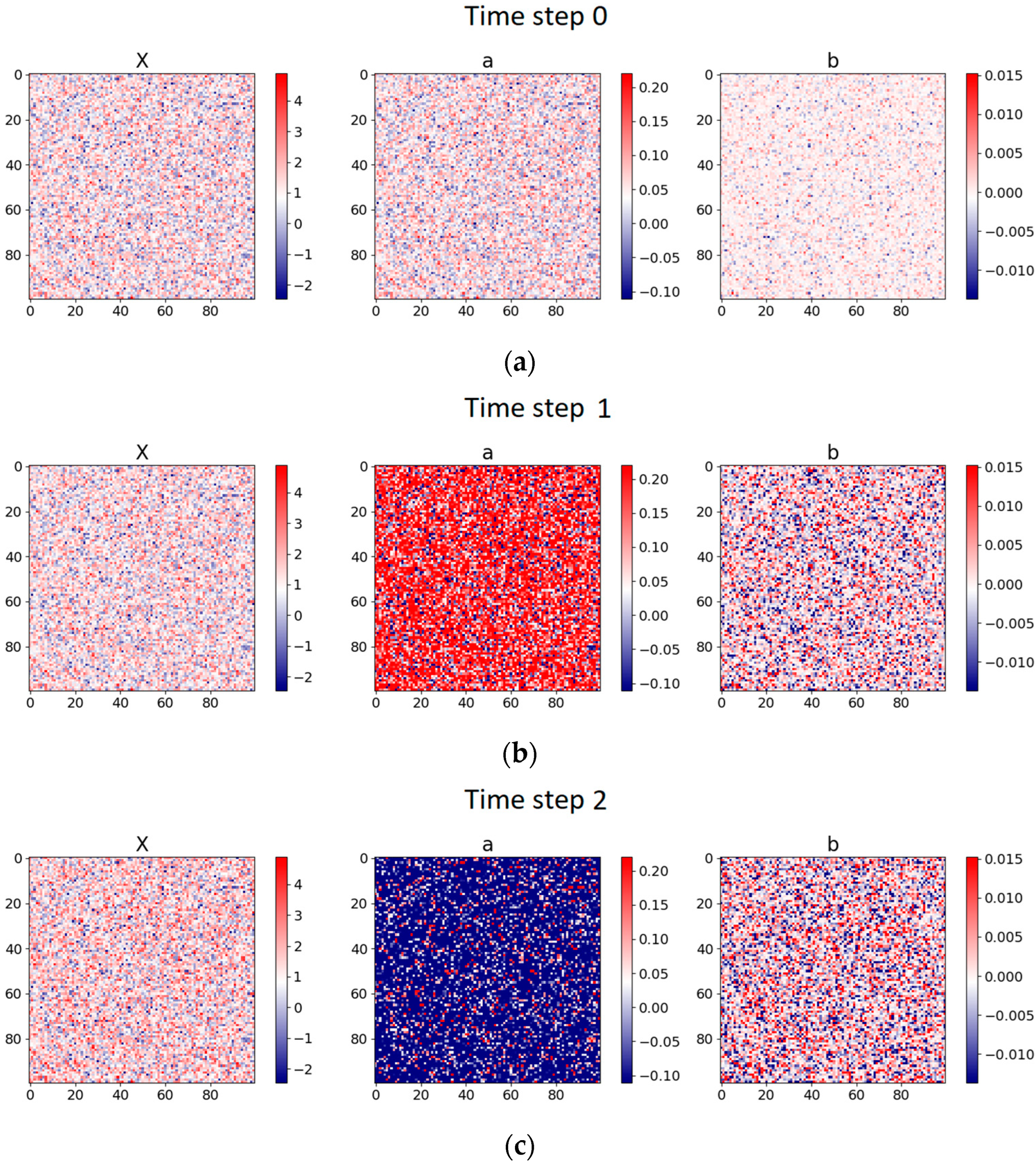
Figure 1 shows the generated triplets of the process values and the corresponding coefficients and at the first three consecutive steps of simulation of the matrices of size . Both methods described in Section 2 are applied to the constructed process, and their resulting estimations of the coefficients are compared with the defined functions and .
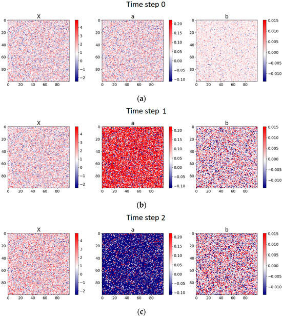
Figure 1.
The values of the simulated stochastic process and the corresponding random coefficients and from the Itô SDE at the three consecutive time steps (iterations): (a), (b), and (c).
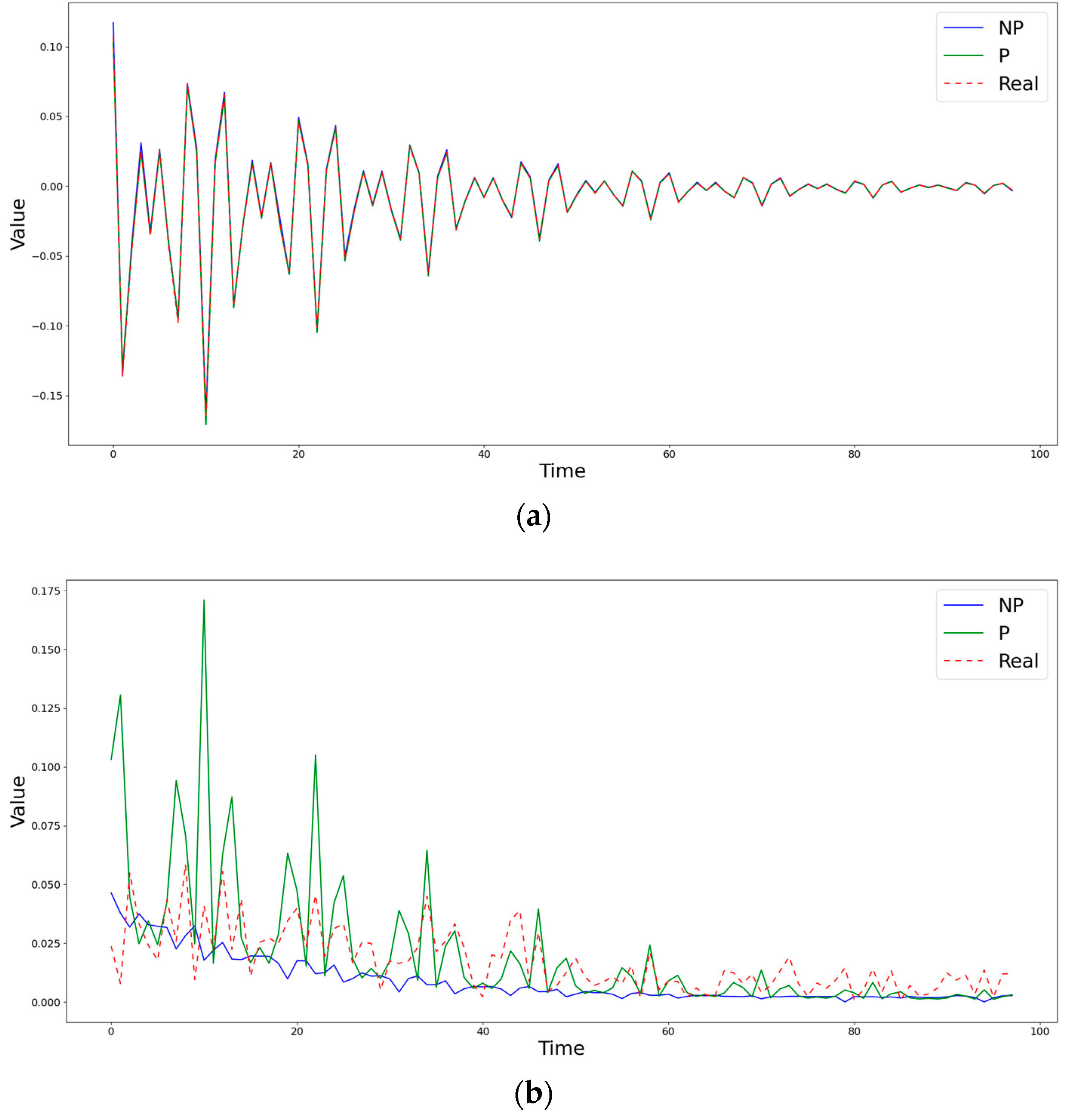
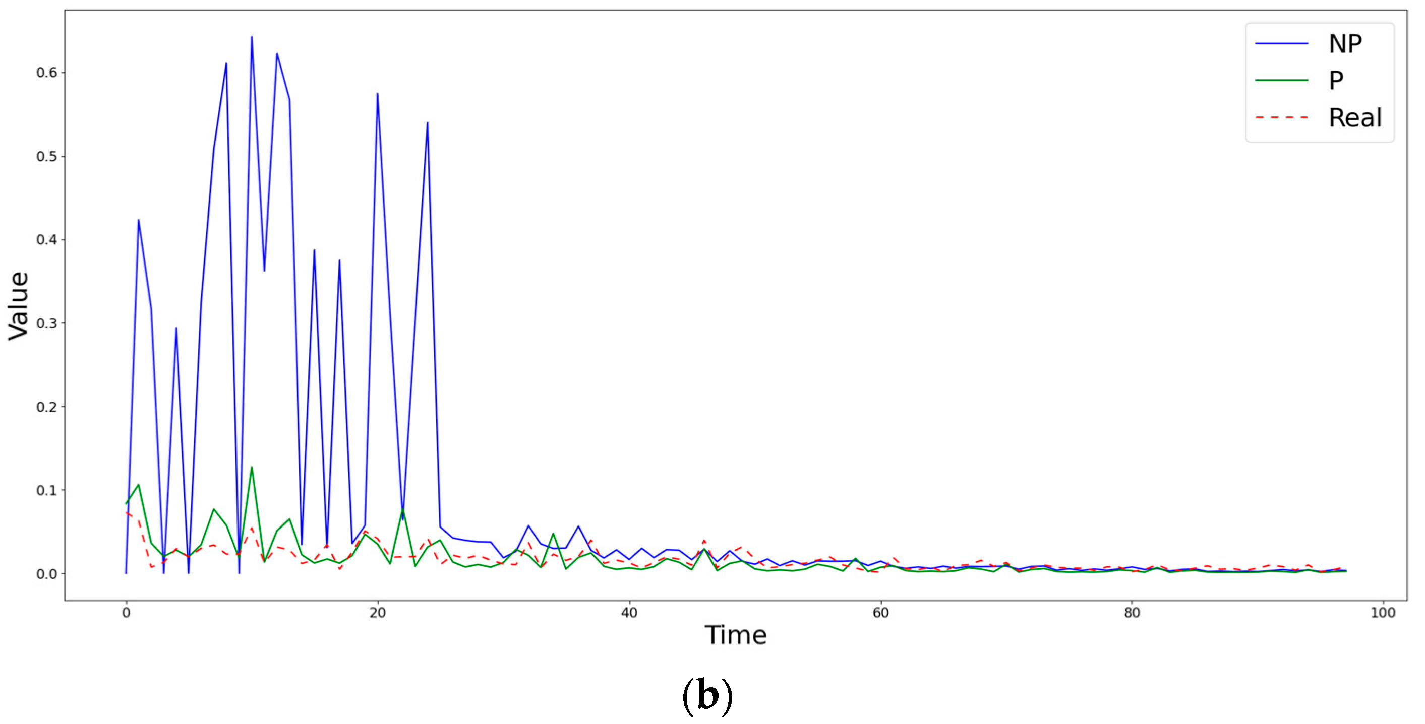
Figure 2, Figure 3 and Figure 4 show the time step evolution of the objective functions and the corresponding estimates obtained by both methods at some fixed points of the matrix (grid nodes), demonstrating the features of both estimation methods. The time axis shows the number of steps of the generation. The data are similar to those in Figure 1, but over a much longer period of time (about 100 iterations).
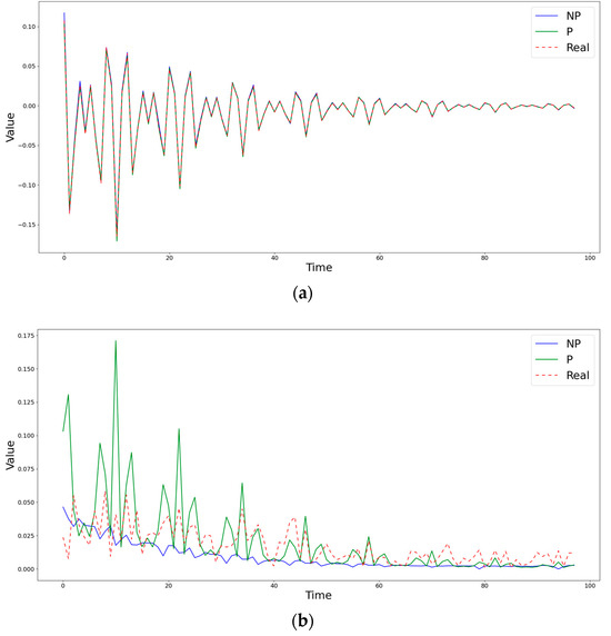
Figure 2.
Comparison of obtained estimates of the coefficients (a) and (b) by nonparametric (NP) and semiparametric (P) methods with the known simulated values at the point (0,4).
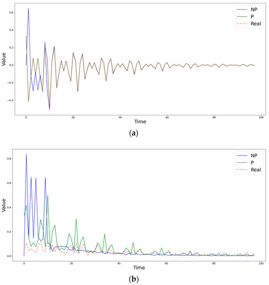
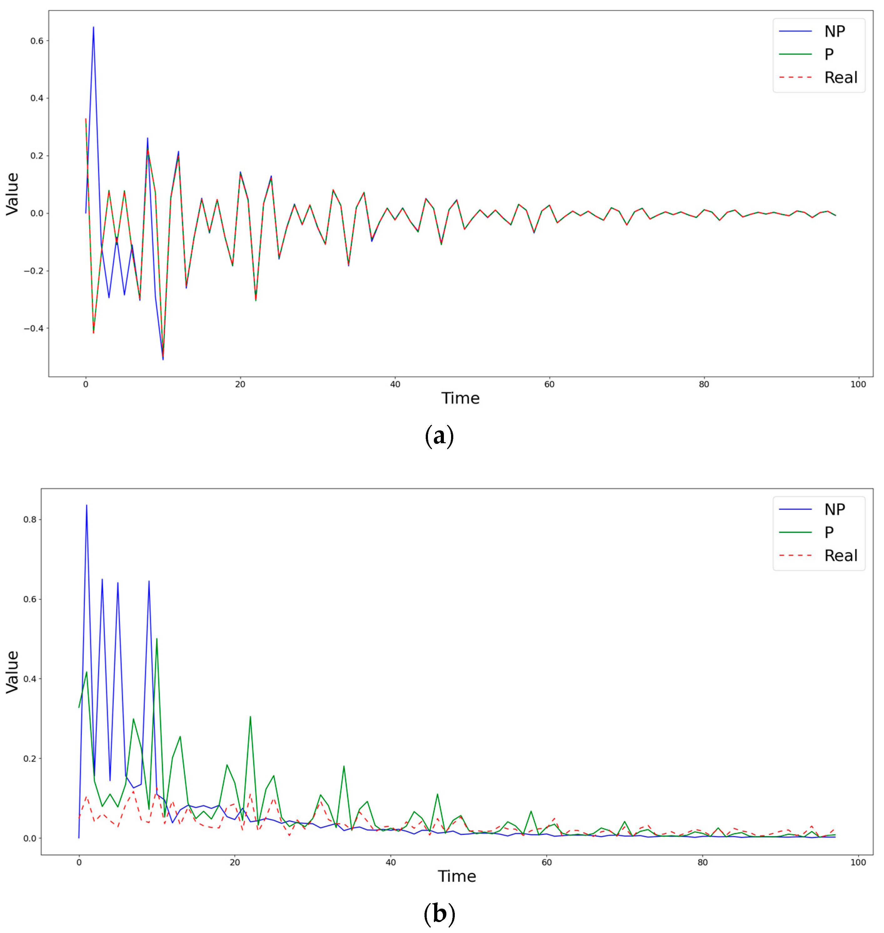
Figure 3.
Comparison of obtained estimates of the coefficients (a) and (b) by nonparametric (NP) and semiparametric (P) methods with the known simulated values at the point (0,11).
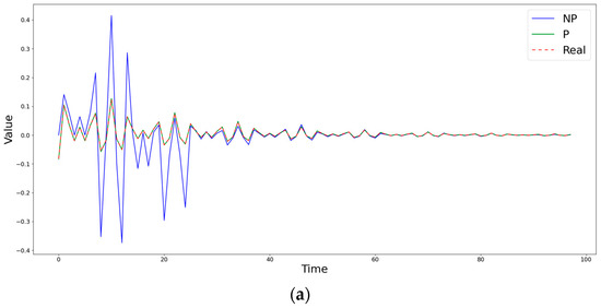

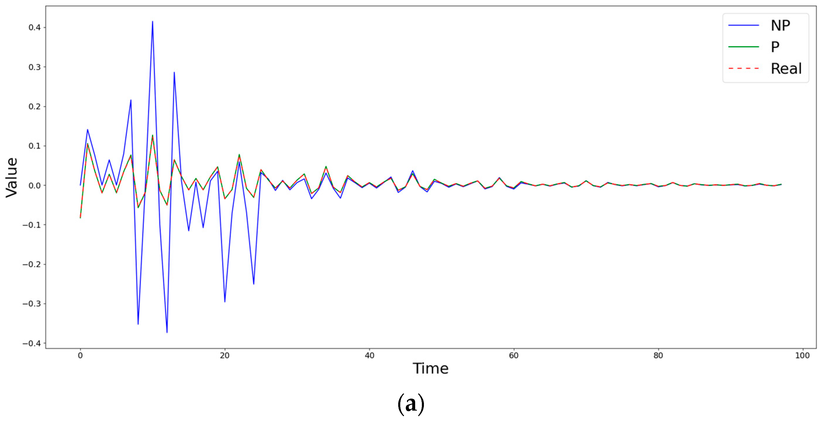
Figure 4.
Comparison of obtained estimates of the coefficients (a) and (b) by nonparametric (NP) and semiparametric (P) methods with the known simulated values at the point (0,27).
Figure 2 demonstrates a case in which the semiparametric method is inferior to the nonparametric one in terms of the RMSE, but captures the behavior of the diffusion coefficient much better. Figure 3 shows a situation in which, during the first steps, both methods differ significantly from the true value of the diffusion coefficient , but, at subsequent time moments, the semiparametric method begins to describe the trend better, significantly surpassing the piecewise linear version of nonparametric estimates. An example of the clear superiority of the semiparametric method is shown in Figure 4.

Table 1.
Errors in coefficient estimation by semiparametric and nonparametric methods.
Table 2.
Errors in coefficient estimation by semiparametric and nonparametric methods.
It is worth noting that the estimates of the drift coefficient obtained by both methods at all considered points of the simulated map are much closer to the real values of the objective functions than the corresponding estimates of the diffusion coefficient to their objective ones.
4. Reanalysis Data Experiments
Now, both methods are applied to the spatiotemporal reanalysis data of the heat fluxes between the ocean and the atmosphere in the North Atlantic for the period 1979–2022. To test and compare the results of the methods on real data, the reanalysis data from the ERA5 database for sensible and latent heat fluxes described in Section 2 are used.
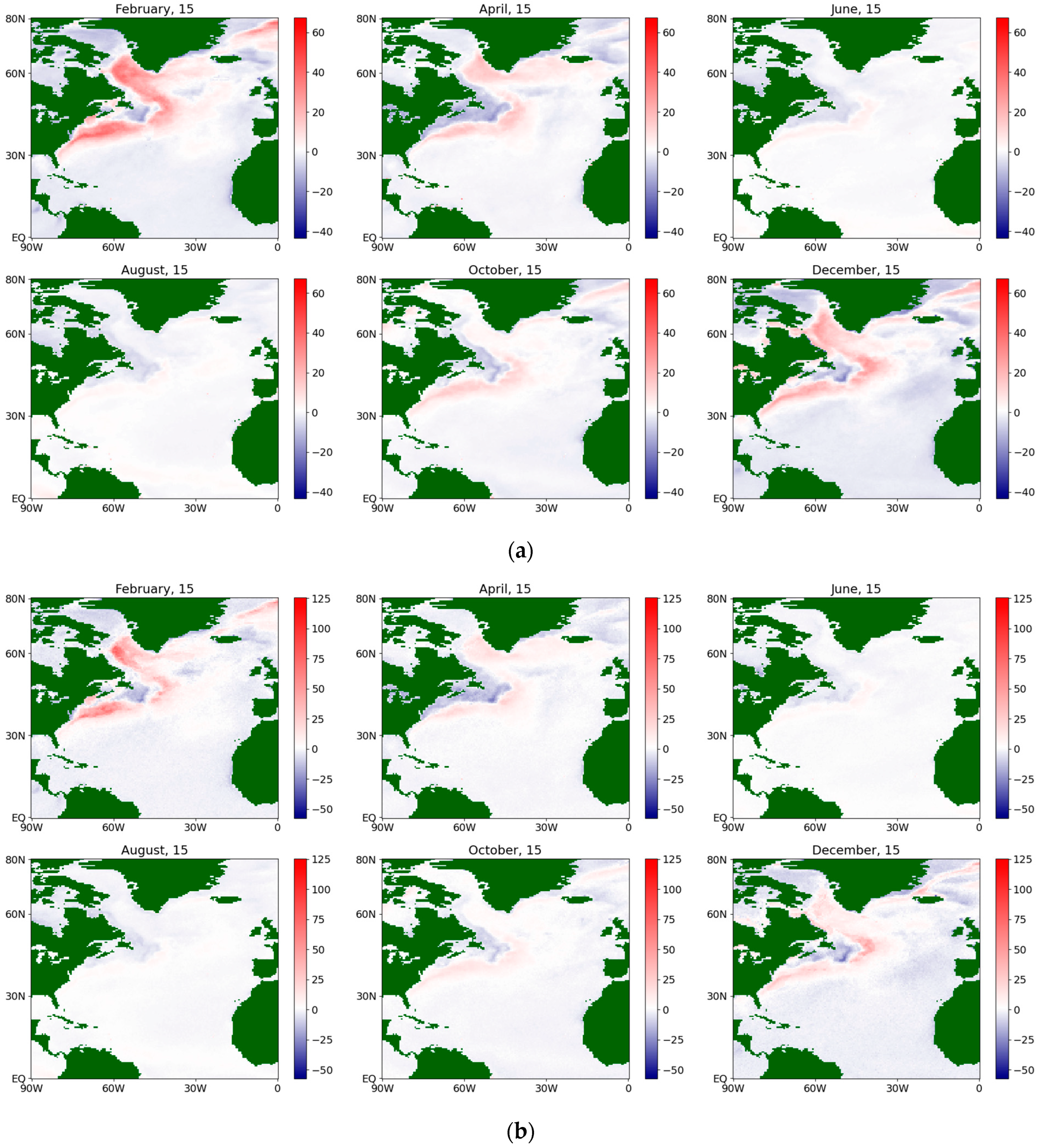
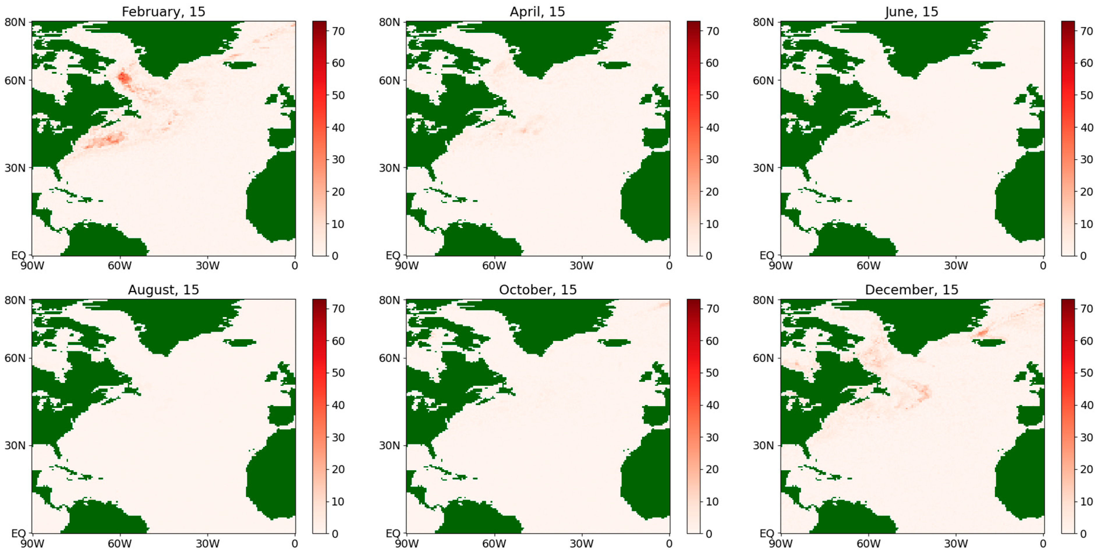
Figure 5, Figure 6, Figure 7 and Figure 8 show the results of both methods for sensible and latent heat fluxes during the so-called “average year”, which are constructed as follows: at each of the six selected fixed days per year in different seasons (namely, February, April, June, August, October, and December), the obtained estimates are averaged for all the considered years. This makes it possible to smooth out individual outliers that arise both directly in the data themselves and due to computational errors during the calculation of point estimates. The results of applying the nonparametric method to the same data and their analysis from the geophysical point of view for this period can be found in the paper [24].
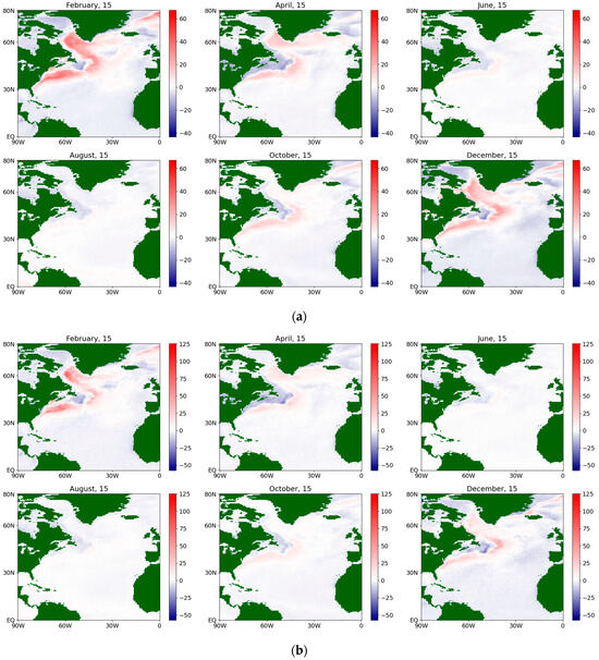
Figure 5.
The estimates of the drift coefficient for the sensible flux during an average year for the period 1979–2022, obtained via a (a) semiparametric method and (b) nonparametric method.
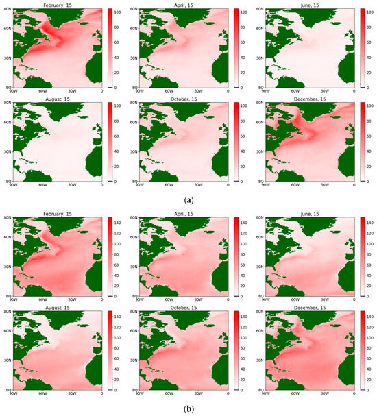
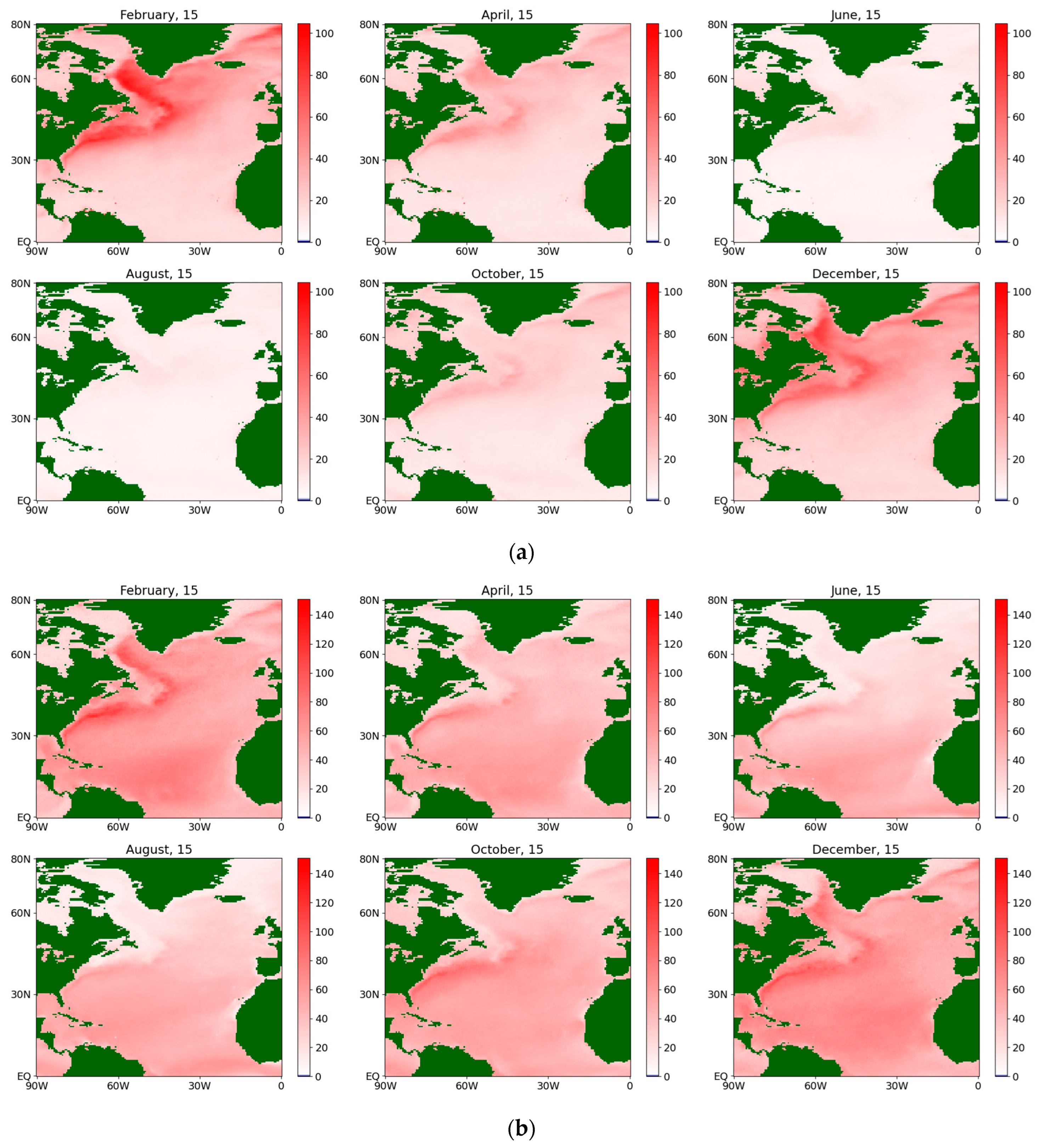
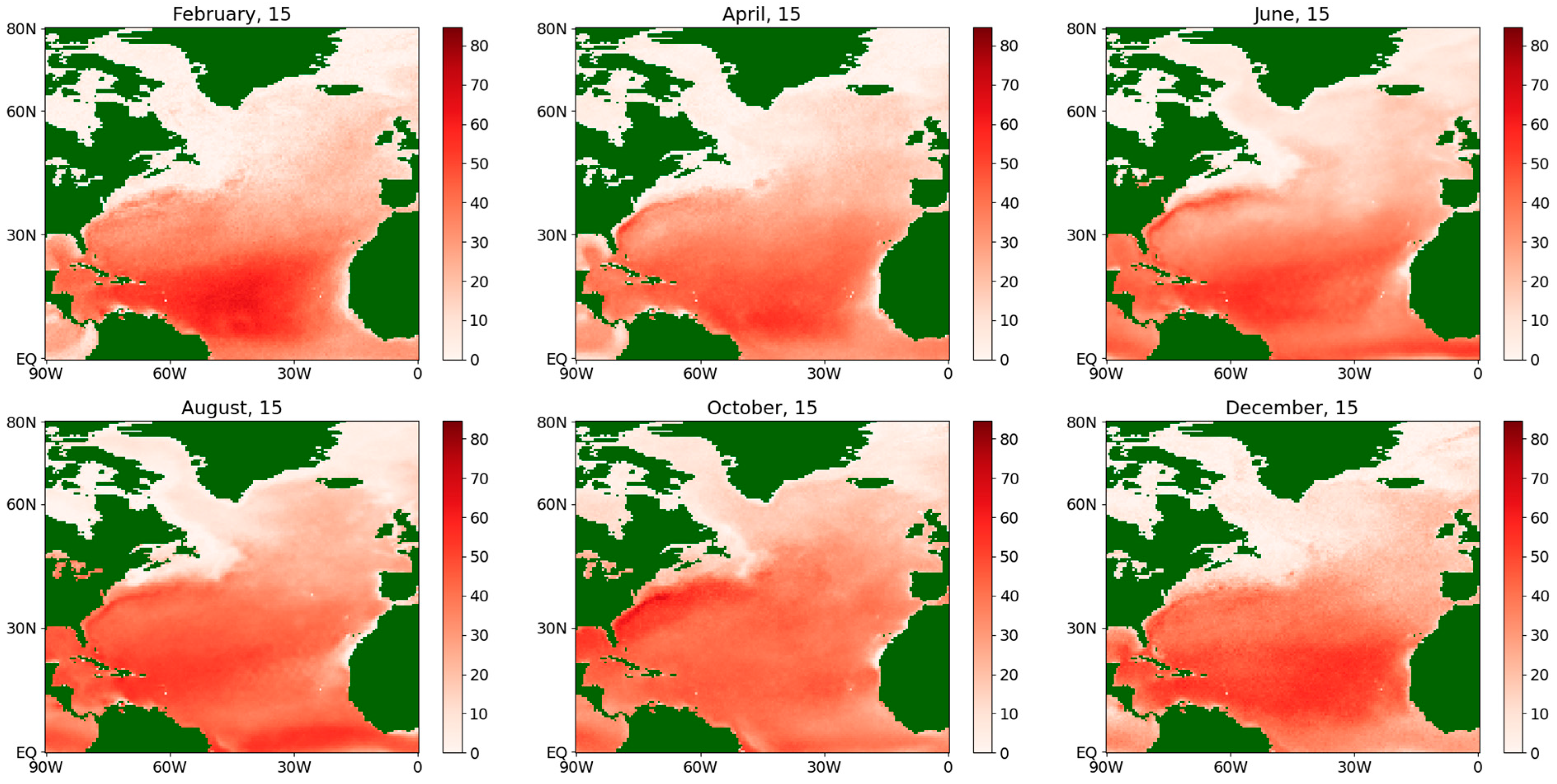
Figure 6.
The estimates of the diffusion coefficient for the sensible flux during an average year for the period 1979–2022, obtained via a (a) semiparametric method and (b) nonparametric method.
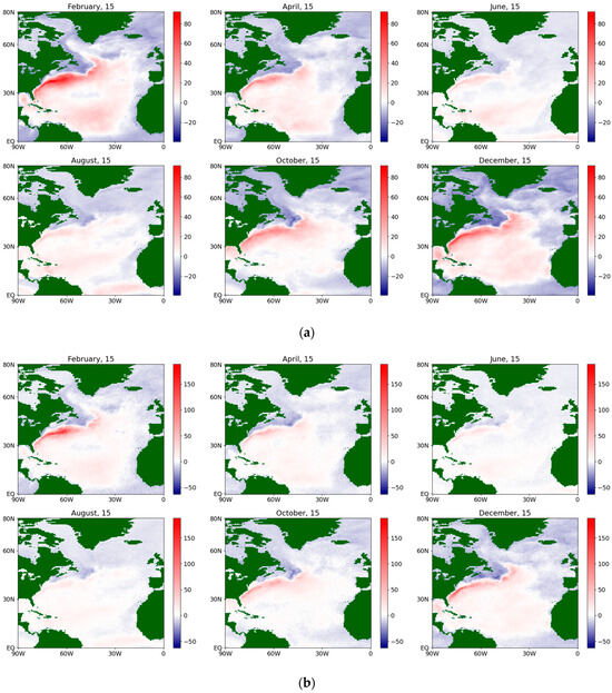
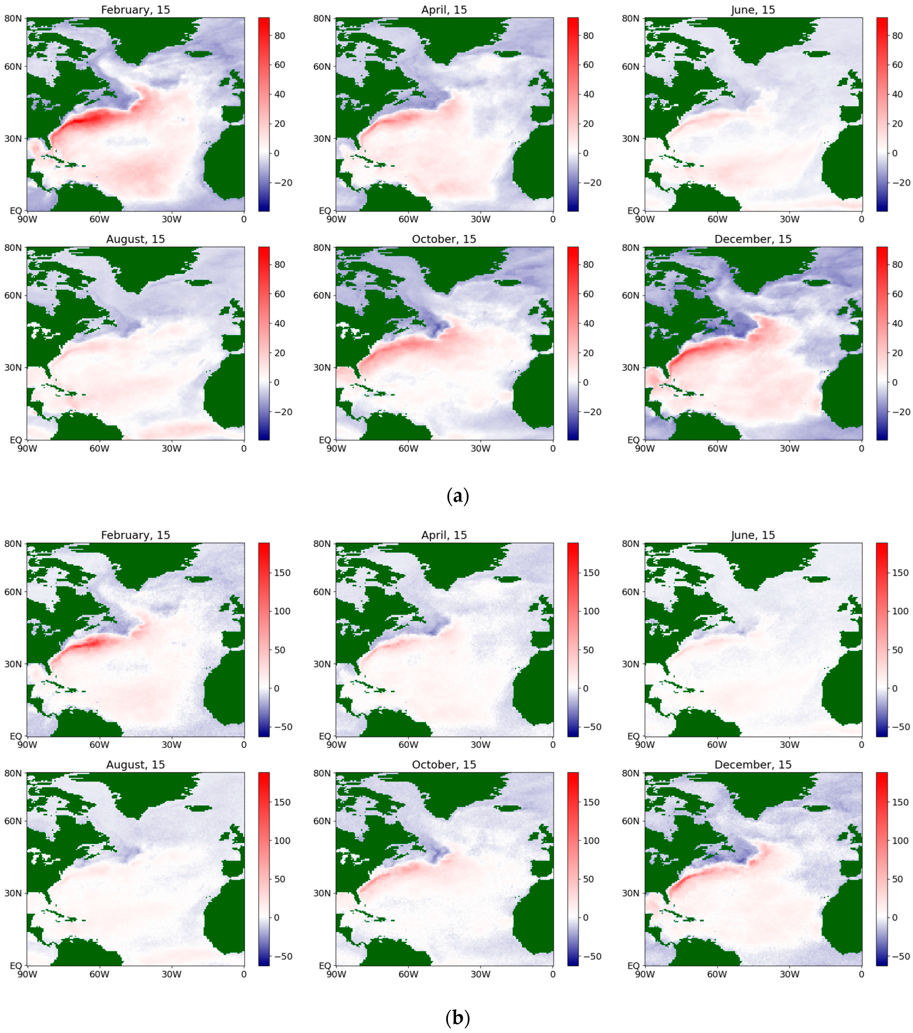
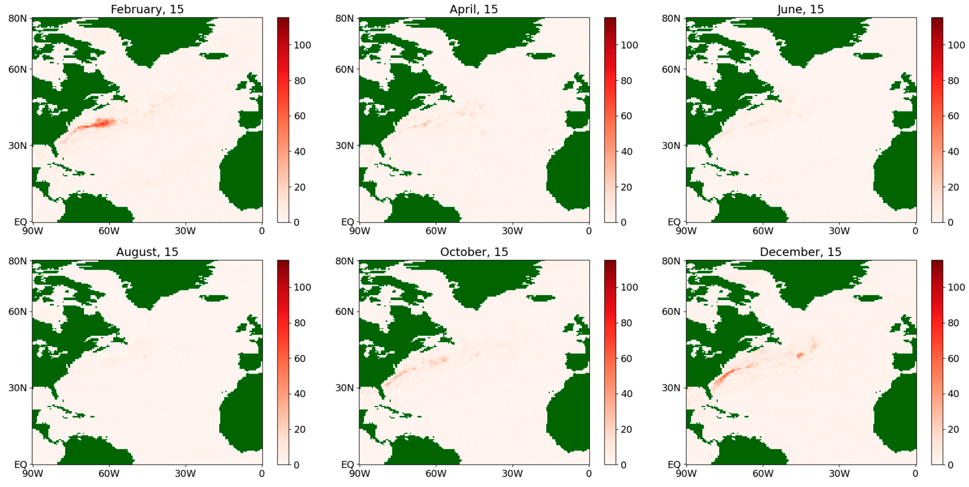
Figure 7.
The estimates of the drift coefficient for the latent flux during an average year for the period 1979–2022, obtained via a (a) semiparametric method and (b) nonparametric method.
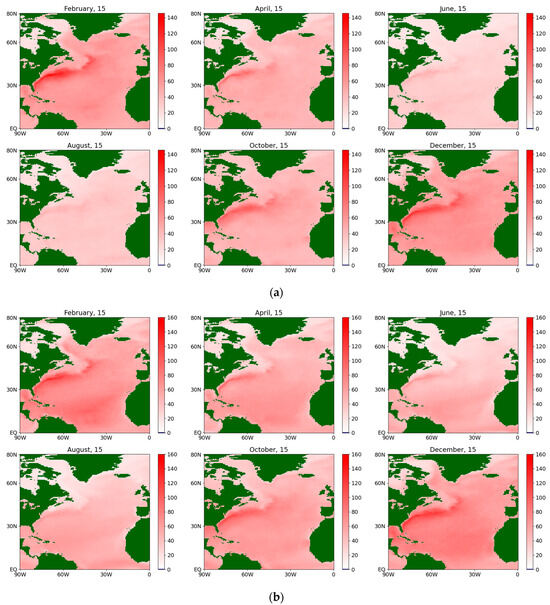
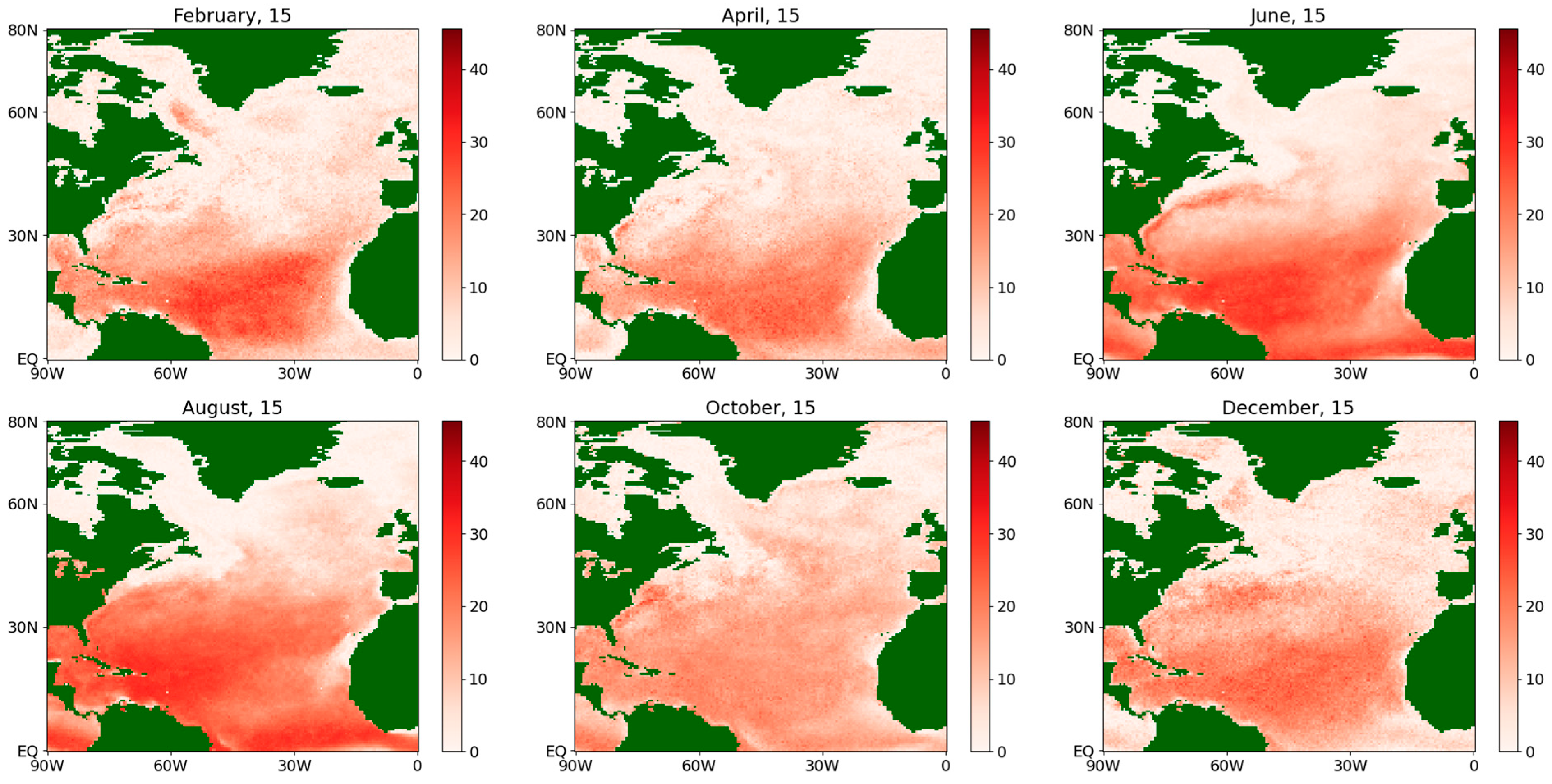
Figure 8.
The estimates of the diffusion coefficient for the latent flux during an average year for the period 1979–2022, obtained via a (a) semiparametric method and (b) nonparametric method.
The color scales on the maps change from blue (for negative values) to white (for values close to zero) and further to red (for positive values). The brightness of the color at a particular point corresponds to the distance of the value from zero. Land areas are marked in dark green. Obviously, on the maps corresponding to the estimates of the diffusion coefficient, the blue color does not appear because the values are non-negative (from a physical point of view, the diffusion coefficient is equivalent to the variance in a random variable).
Figure 5 shows an example of the values of the obtained estimates obtained from both methods for the drift coefficient for the sensible flux during an average year. It can be seen that, visually, they coincide very strongly, but the estimates obtained by the semiparametric method change color more smoothly in the neighboring nodes of the map (that is, they have closer values) and also have values in the peak areas that are smaller in absolute terms than the corresponding ones obtained by using the nonparametric method. The trend in the maximum absolute values, as expected, corresponds well to the zones of strong jet streams in the North Atlantic. A seasonal cycle is also observed: in the winter months, the drift coefficient is positive, whereas, in the summer months, it is negative.
The localization obtained via the nonparametric method is coarser and more explicit, but less detailed than that obtained via the semiparametric method. Similar conclusions are also valid for the diffusion coefficient (see Figure 6), although the mentioned effect turns out to be less pronounced. It is characterized by extensive zones of its maximum value and a less pronounced seasonal cycle than for the corresponding drift coefficient, although in the summer months the maximum is noticeably smaller in both methods for both sensible and latent fluxes. Figure 7 and Figure 8 present the same coefficients for the latent fluxes.
For a vivid comparison of the results obtained by both methods for the entire North Atlantic area at once, the values of the absolute differences of estimates at each point of the half-degree grid are presented in Figure 9, Figure 10, Figure 11 and Figure 12. The format of an average year is used again.
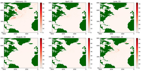
Figure 9.
Absolute difference of the estimates of the drift coefficient for the sensible flux during an average year for the period 1979–2022.
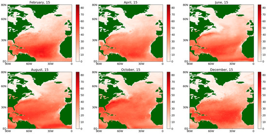
Figure 10.
Absolute difference of the estimates of the diffusion coefficient for the sensible flux during an average year for the period 1979–2022.
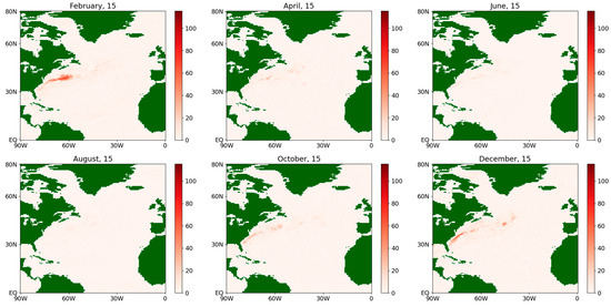
Figure 11.
Absolute difference of the estimates of the drift coefficient for the latent flux during an average year for the period 1979–2022.
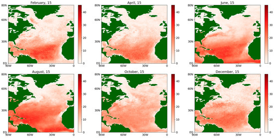
Figure 12.
Absolute difference of the estimates of the diffusion coefficient for the latent flux during an average year for the period 1979–2022, obtained by using both.
For the drift coefficients for the fluxes of both types, some significant differences in the results of the methods are observed along the Gulf Stream (see Figure 9 and Figure 11) while, for the rest of the map, the differences can appear due to computational error reasons.
At the same time, the difference between the obtained values for the diffusion coefficient is seen much more clearly (see Figure 10 and Figure 12), especially for the winter and spring of an average year in more northern latitudes, as well as in the Gulf Stream region. This fact may be explained as follows. In northern latitudes, there are more random factors that determine the ocean–atmosphere interaction due to a larger temperature spread and stronger winds, which determine the emerging fluxes to a large extent. This is one of the most important arguments in favor of the more accurate semiparametric estimation procedure (see Section 3.4).
5. Conclusions and Discussion
The paper presents research on applying the semiparametric method for reconstructing random drift and diffusion coefficients of the Itô SDE and comparing this method with the nonparametric method, using both synthetically generated data and the reanalysis data of the sensible and latent heat fluxes in the North Atlantic for the period 1979–2022 from the ERA5 database.
The advantages of nonparametric procedures include the possibility of theoretical proof of the properties of the estimates, for example, their consistency, including for the multidimensional case. However, this method requires a few additional assumptions. A semiparametric reconstruction procedure is free from them. Only the existence of a solution to the stochastic differential equation is needed. However, this method is oriented on samples of limited volume (windows), which imposes restrictions on the possibility to prove asymptotic statistical properties. An empirical comparison of both methods in the paper, however, shows the similarity of their results, which indicates the possibility of using these methods for applied mathematical modeling.
The conclusions are as follows:
- The methods used for estimating the parameters of the Itô equation coefficients for the proposed model of heat flux dynamics are adequate, provide mathematically and physically justified results, and are in good agreement with the physical features of the heat fluxes in the North Atlantic;
- Accuracy estimates with respect to the simulated series give acceptable interval values (mean value is about , whereas the variability in the series itself equals ) and reflect the trends in the test series well. The semiparametric approach is usually more accurate for data under stochastic factors, but it has a higher computational complexity than a simple interval method of frequency nonparametric estimates. The typical running times of the methods at one time step were s and s, respectively;
- The areas of maximum absolute values of the drift coefficient correspond well to the areas of strong jet streams in the North Atlantic and have a noticeable seasonal variation. In the winter months, the coefficient is positive; in the summer months, it is negative. The localization obtained by the nonparametric method is coarser and more explicit, but less detailed than that from the semiparametric method. Similar conclusions are also valid for the diffusion coefficient, although, in the summer months, the maximum is noticeably smaller in both methods for both the sensible and latent heat fluxes.
Thus, the following problems can be mentioned as possible directions of the further research:
- The proposed semiparametric approach can be extended for analyzing multivariate distributions, to study the relationship between heat fluxes, pressure, and sea-surface temperature;
- The stochastic models for the data increments may also be in demand in completely different applied areas, for example, in turbulent plasma physics. The semiparametric approach is suitable for this type of data. This opens up new prospects for physics-informed ML models [25,26,27,28], including those based on SDEs [29,30,31,32].
Author Contributions
Conceptualization, A.K.G., K.P.B. and V.Y.K.; methodology, A.K.G., K.P.B. and V.Y.K.; software, A.A.O.; validation, K.P.B., A.K.G., V.Y.K. and A.A.O.; formal analysis, A.A.O., K.P.B., A.K.G. and V.Y.K.; investigation, A.A.O., A.K.G., K.P.B. and V.Y.K.; resources, A.A.O. and A.K.G.; data curation, A.A.O.; writing—original draft preparation, A.K.G., A.A.O., K.P.B. and V.Y.K.; writing—review and editing, A.K.G., A.A.O. and K.P.B.; visualization, A.A.O.; supervision, A.K.G.; project administration, A.K.G.; funding acquisition, A.K.G. All authors have read and agreed to the published version of the manuscript.
Funding
This research was supported by the Russian Science Foundation (grant No 22-11-00212).
Data Availability Statement
Data are contained within the article.
Acknowledgments
The research was carried out using the infrastructure of the Shared Research Facilities “High Performance Computing and Big Data” (CKP “Informatics”) of the Federal Research Center “Computer Science and Control” of the Russian Academy of Sciences.
Conflicts of Interest
The authors declare no conflicts of interest.
References
- Perry, A.H.; Walker, J.M. The Ocean-Atmosphere System; Longman: London, UK; New York, NY, USA, 1977. [Google Scholar]
- Pascucci, A.; Pesce, A. On Stochastic Langevin and Fokker-Planck Equations: The Two-Dimensional Case. J. Differ. Equ. 2022, 310, 443–483. [Google Scholar] [CrossRef]
- Yoshida, N. Estimation for Diffusion Processes from Discrete Observation. J. Multivar. Anal. 1992, 41, 220–242. [Google Scholar] [CrossRef]
- Genon-Catalot, V.; Jacod, J. On the Estimation of the Diffusion Coefficient for Multi-Dimensional Diffusion Processes. Ann. L’I.H.P. Probab. Stat. 1993, 29, 119–151. [Google Scholar]
- Genon-Catalot, V.; Jacod, J. Estimation of the Diffusion Coefficient for Diffusion Processes: Random Sampling. Scand. J. Stat. 1994, 21, 193–221. [Google Scholar]
- Wei, C.; Shu, H. Maximum Likelihood Estimation for the Drift Parameter in Diffusion Processes. Stochastics 2016, 88, 699–710. [Google Scholar] [CrossRef]
- Florens-Zmirou, D. On Estimating the Diffusion Coefficient from Discrete Observations. J. Appl. Probab. 1993, 30, 790–804. [Google Scholar] [CrossRef]
- Lamouroux, D.; Lehnertz, K. Kernel-Based Regression of Drift and Diffusion Coefficients of Stochastic Processes. Phys. Lett. A 2009, 373, 3507–3512. [Google Scholar] [CrossRef]
- Belyaev, K.P.; Korolev, V.Y.; Gorshenin, A.K.; Antipov, A.I.; Imeev, M.A.; Kirushkin, N.I.; Lobovskii, M.A. Some Features of the Intra-Annual Variability of Heat Fluxes in the North Atlantic. Izv. Atmos. Ocean. Phys. 2021, 57, 619–631. [Google Scholar] [CrossRef]
- Budyko, M.I. Climate Changes; Gidrometeoizdat: Leningrad, Russia, 1974. [Google Scholar]
- Hasselmann, K. Stochastic Climate Models: Part I. Theory. Tellus A Dyn. Meteorol. Oceanogr. 1976, 28, 473. [Google Scholar] [CrossRef]
- van den Berk, J.; Drijfhout, S.; Hazeleger, W. Characterisation of Atlantic Meridional Overturning Hysteresis Using Langevin Dynamics. Earth Syst. Dyn. 2021, 12, 69–81. [Google Scholar] [CrossRef]
- Toppaladoddi, S.; Wells, A.J. A Stochastic Model for the Turbulent Ocean Heat Flux under Arctic Sea Ice. arXiv 2021, arXiv:2108.11815. [Google Scholar] [CrossRef]
- Voutilainen, M.; Viitasaari, L.; Ilmonen, P.; Torres, S.; Tudor, C. Vector-valued Generalized Ornstein–Uhlenbeck Processes: Properties and Parameter Estimation. Scand. J. Stat. 2022, 49, 992–1022. [Google Scholar] [CrossRef]
- Belyaev, K.P.; Gorshenin, A.K.; Korolev, V.Y.; Plekhanov, A. Statistical Analysis of Intra- and Interannual Variability of Extreme Values of Sensible and Latent Heat Fluxes in the North Atlantic for 1979–2021. Izv. Atmos. Ocean. Phys. 2022, 58, 609–624. [Google Scholar] [CrossRef]
- Gorshenin, A.K.; Kuzmin, V.Y. Statistical Feature Construction for Forecasting Accuracy Increase and Its Applications in Neural Network Based Analysis. Mathematics 2022, 10, 589. [Google Scholar] [CrossRef]
- Gikhman, I.; Skorokhod, A.V. The Theory of Stochastic Processes II; Springer: Berlin/Heidelberg, Germany, 2004. [Google Scholar]
- Cronin, M.F.; Gentemann, C.L.; Edson, J.; Ueki, I.; Bourassa, M.; Brown, S.; Clayson, C.A.; Fairall, C.W.; Farrar, J.T.; Gille, S.T.; et al. Air-Sea Fluxes With a Focus on Heat and Momentum. Front. Mar. Sci. 2019, 6, 430. [Google Scholar] [CrossRef]
- Leyba, I.M.; Solman, S.A.; Saraceno, M. Trends in Sea Surface Temperature and Air–Sea Heat Fluxes over the South Atlantic Ocean. Clim. Dyn. 2019, 53, 4141–4153. [Google Scholar] [CrossRef]
- Belyaev, K.; Kuleshov, A.; Tuchkova, N.; Tanajura, C.A.S. An Optimal Data Assimilation Method and Its Application to the Numerical Simulation of the Ocean Dynamics. Math. Comput. Model. Dyn. Syst. 2018, 24, 12–25. [Google Scholar] [CrossRef]
- Shiryaev, A.; Bulinsky, A.V. Theory of Random Processes; FIZMATLIT: Moscow, Russia, 2005. [Google Scholar]
- Teicher, H. Identifiability of Mixtures. Ann. Math. Stat. 1961, 32, 244–248. [Google Scholar] [CrossRef]
- McLachlan, G.J.; Krishnan, T. The EM Algorithm and Extensions; John Wiley & Sons: Hoboken, NJ, USA, 2007. [Google Scholar]
- Gorshenin, A.K.; Osipova, A.A.; Belyaev, K.P. Stochastic Analysis of Air–Sea Heat Fluxes Variability in the North Atlantic in 1979–2022 Based on Reanalysis Data. Comput. Geosci. 2023, 181, 105461. [Google Scholar] [CrossRef]
- Karniadakis, G.E.; Kevrekidis, I.G.; Lu, L.; Perdikaris, P.; Wang, S.; Yang, L. Physics-Informed Machine Learning. Nat. Rev. Phys. 2021, 3, 422–440. [Google Scholar] [CrossRef]
- Raissi, M.; Perdikaris, P.; Karniadakis, G.E. Physics-Informed Neural Networks: A Deep Learning Framework for Solving Forward and Inverse Problems Involving Nonlinear Partial Differential Equations. J. Comput. Phys. 2019, 378, 686–707. [Google Scholar] [CrossRef]
- Subramanian, A.; Mahadevan, S. Probabilistic Physics-Informed Machine Learning for Dynamic Systems. Reliab. Eng. Syst. Saf. 2023, 230, 108899. [Google Scholar] [CrossRef]
- Fuhg, J.N.; Bouklas, N. On Physics-Informed Data-Driven Isotropic and Anisotropic Constitutive Models through Probabilistic Machine Learning and Space-Filling Sampling. Comput. Methods Appl. Mech. Eng. 2022, 394, 114915. [Google Scholar] [CrossRef]
- Sugishita, N.; Ohkubo, J. Embedding Stochastic Differential Equations into Neural Networks via Dual Processes. J. Stat. Mech. Theory Exp. 2023, 2023, 093201. [Google Scholar] [CrossRef]
- Xu, W.; Chen, R.T.; Li, X.; Duvenaud, D. Infinitely Deep Bayesian Neural Networks with Stochastic Differential Equations. In Proceedings of the International Conference on Artificial Intelligence and Statistics, Virtual, 28–30 March 2022; pp. 721–738. [Google Scholar]
- Beck, C.; Becker, S.; Grohs, P.; Jaafari, N.; Jentzen, A. Solving Stochastic Differential Equations and Kolmogorov Equations by Means of Deep Learning. arXiv 2018, arXiv:1806.00421. [Google Scholar]
- Yang, L.; Zhang, D.; Karniadakis, G.E. Physics-Informed Generative Adversarial Networks for Stochastic Differential Equations. SIAM J. Sci. Comput. 2020, 42, A292–A317. [Google Scholar] [CrossRef]

Disclaimer/Publisher’s Note: The statements, opinions and data contained in all publications are solely those of the individual author(s) and contributor(s) and not of MDPI and/or the editor(s). MDPI and/or the editor(s) disclaim responsibility for any injury to people or property resulting from any ideas, methods, instructions or products referred to in the content. |
© 2024 by the authors. Licensee MDPI, Basel, Switzerland. This article is an open access article distributed under the terms and conditions of the Creative Commons Attribution (CC BY) license (https://creativecommons.org/licenses/by/4.0/).