Abstract
In recent years, the global resource shortage has become a serious issue. Recycling end-of-life (EOL) products is conducive to resource reuse and circular economy and can mitigate the resource shortage issue. The disassembly of EOL products is the first step for resource reuse. Disassembly activities need tools, and tool deterioration occurs inevitably during the disassembly process. This work studies the influence of tool deterioration on disassembly efficiency. A disassembly line balancing model with the goal of maximizing disassembly profits is established, in which tool selection and assignment is a critical part. A modified discrete migratory bird optimizer is proposed to solve optimization problems. The well-known IBM CPLEX optimizer is used to verify the correctness of the model. Six real-world products are used for disassembly experiments. The popular fruit fly optimization algorithm, whale optimization algorithm and salp swarm algorithm are used for search performance comparison. The results show that the discrete migratory bird optimizer outperforms all three other algorithms in all disassembly instances.
Keywords:
disassembly line balancing problem; tool deterioration; migratory bird optimizer; genetic operators MSC:
68T20
1. Introduction
Over the years, a large quantity of EOL products have been accumulating. There are many useful parts in these products, and recycling and reusing them is an important part of the development of the circular economy. Disassembly is an important means to product recycling [1,2,3], and the structure of the disassembly line is shown in Figure 1. However, in the process of disassembly, the wear degree of disassembly tools and the execution order of tasks can lead to different disassembly times for tasks on the workstations, which affects the efficiency of disassembly. Considering these factors, a good disassembly scheme is very important for the recovery of EOL products [4,5,6,7]. In order to solve this problem, many researchers have studied the disassembly line balancing problem (DLBP).

Figure 1.
Disassembly line construction.
Since DLBP was officially introduced by Gungor et al. in 2001 [8], researchers have tried to solve DLBP by various methods. McGovern and Gupta [9] prove that DLBP is an NP-complete problem. As the problem size increases slightly, the number of calculations required to determine the optimality of a solution increases exponentially, whereupon it is impossible to obtain the optimal solution in an acceptable time. At present, intelligent optimization algorithms are widely used in solving DLBP because of their fast convergence speed and strong robustness. McGovern and Gupta [9] propose a new formula for quantifying the level of balancing and solve the problem with a genetic algorithm. Kalayci and Gupta [10] propose a particle swarm optimization algorithm based on a neighborhood mutation operator to solve this problem. Tuncel et al. [11] use a Monte-Carlo-based reinforcement learning technique to solve DLBP. Liu et al. [12] propose an improved discrete artificial bee colony algorithm to solve the sequence-dependent disassembly line balancing problem. Hu et al. [13] aim at reducing energy consumption and propose an improved ant colony optimization algorithm to optimize the disassembly sequence. Guo et al. [14] use various heuristic algorithms to solve the multi-objective optimization problem of the disassembly line.
In the actual disassembly process, the processing time of the disassembly task is affected by many factors. The functional deterioration of disassembly tools is one of them. Tool deterioration causes the actual processing time of disassembly tasks to grow longer over time [15,16,17]. Some studies are reported that consider tool deterioration in manufacturing systems. For example, in [18], a scheduling model with deteriorating characteristics is proposed. In this model, the authors define the processing time of the job as a linear increasing function of its start time. In [19], Ng et al. compare the linear functions of the decreasing and increasing processing times of the workpieces, which prove that the two linear models are closely related. Cheng and Sun [20] prove that the total weighted completion time problem is NP-hard. The above research is carried out for single-machine scheduling. Toksarı and Güner [21] define the processing time of a job as a function of the execution start time of the job and its position in the sequence, which is used to solve the scheduling problem of advance or delay in parallel machines. Wang et al. [22] propose two heuristic algorithms to solve a two-machine flow shop scheduling problem with deterioration and learning effects. Behnamian [23] studies the impact of learning and degradation on the hybrid flowshop scheduling with sequence-dependent setup time.
To the best of our knowledge, there is no research reported so far on the tool deterioration in the scheduling and performance analysis of DLBP. In the actual disassembly line, however, the deterioration effect cannot be ignored. This work studies DLBP with tool deterioration. When product subassemblies are disassembled with worn tools, the disassembly time will be prolonged. The prolonged time is called deterioration time. We say that the tools have deterioration characteristics, and use the deterioration coefficient to represent the influence degree of tool deterioration on the disassembly time.
On the other hand, DBLP is an NP-hard problem, and in many cases, we have to rely on heuristic search to find the optimal solution to DBLP. The migratory bird optimizer (MBO) is a heuristic optimization algorithm based on the migration behavior of migratory birds that simulates the strategies and behaviors of the migratory bird population during the migration process. MBO has a strong global search ability that can help find the global optimal solution or approximate the optimal solution to a problem. MBO has high robustness and can adapt to diverse problem domains and complex optimization problems. Compared to some complex optimization algorithms, the implementation of the migratory bird optimization algorithm is relatively simple and does not require a large amount of parameter adjustment and problem specific knowledge. This makes the algorithm easy to understand, implement and apply [24]. At present, it has been applied to the stochastic disassembly line balancing problems [25], scheduling problems [26,27], knapsack problems [28], system identification problems [29] and quadratic assignment problems [30]. In this work, we choose to use MBO to solve DLBP with tool deterioration. More specifically, considering the impact of tool deterioration on the disassembly profits, we design a sequence-dependent disassembly line [31] and use the discrete migratory bird optimizer (DMBO) to solve DLBP with tool deterioration.
Compared with the existing studies, we have made the following contributions:
- (1)
- We consider the impact of tool deterioration on disassembly efficiency; a linear disassembly line balancing model is established to rationally allocate tasks on the workstations and optimize disassembly profit.
- (2)
- For DLBP with tool deterioration, we propose a discrete migratory bird optimizer. In this algorithm, we use a two-stage coding method to represent the solution and design three search methods to help the birds update, which can find the optimal solution faster.
- (3)
- We use CPLEX to verify the correctness of the model. By comparing the experimental results of DMBO and other intelligent optimization algorithms, we confirmed that DMBO has excellent performance in solving the presented DBLP.
This work is an extension of our previous work reported in [32], a conference paper, with significant improvements. First, according to the characteristics of DLBP with tool deterioration, we established a mathematical model to maximize the disassembly profit and verify the model with CPLEX to ensure the accuracy of the model [33]. Second, we chose three popular intelligent optimization algorithms to compare with DMBO and verified that DMBO has excellent optimization performance. Finally, we added more experimental cases to make the experimental results more convincing. In addition, we also compared the experimental results of whether tool deterioration is considered, which proves that it is necessary to consider the impact of tool deterioration in DLBP.
The rest of this work is organized as follows. In Section 2, DLBP with tool deterioration is described, and the mathematical model is established. In Section 3, the flow of the DMBO algorithm is introduced. Section 4 shows six experimental cases and the results of comparative experiments. In Section 5, we provide a summary and outlook.
2. Problem Description and Modeling
2.1. Problem Description
DLBP aims to disassemble EOL products on disassembly lines and obtain subassemblies by performing a series of disassembly tasks. For these disassembly tasks, we should reasonably allocate them to workstations on the basis of meeting the constraints of task precedence relation and workstation cycle time, and constantly optimize the disassembly scheme to find the solution that best meets our goals.
A single product linear disassembly line consists of a limited number of workstations with multiple disassembly locations on each workstation. When an EOL product is disassembled, disassembly tasks are assigned to each workstation in turn. For tasks assigned to one workstation, locations are used to indicate their order. Each workstation is equipped with disassembly tools required by the disassembly tasks.
In many studies on DLBP, the disassembly time of subassemblies is constant, and the disassembly task is allocated according to the cycle time of the workstation. As shown in Figure 2, the profit of this disassembly scheme is 185. However, in the actual disassembly process, the tools will be worn to varying degrees after long-term use, resulting in an increase in the disassembly time of subassemblies with the in-use time of tools, increasing the disassembly cost. If we still execute the scheme in Figure 2 after the tool is worn, because both task 1 and task 15 need to use tool 1, when using tool 1 to execute task 1 and then using it to execute task 15, the disassembly time of task 15 is extended by 4.4 due to the deterioration characteristics of tool 1, resulting in a deterioration cost of 22. Therefore, we consider the tool deterioration when formulating the disassembly plan, so as to maximize the disassembly profits.
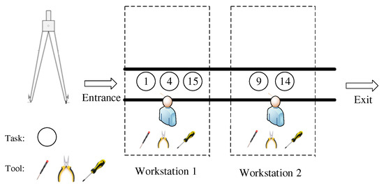
Figure 2.
Disassembly scheme without considering tool deterioration.
2.2. Disassembly Sequence
As in other process-oriented system studies, formal modeling of disassembly processes is always desired [34]. In this work, we use the AND/OR graph to describe the disassembly process of EOL products. The AND/OR graph can not only obtain the precedence and conflict relationship of disassembly tasks but also obtain the relationship between disassembly tasks and subassemblies. The necessity of an AND/OR graph in disassembly planning lies in representing the sequential relationships between the operations or tasks involved in the disassembly process. It helps to determine the order of disassembly of subassemblies based on their subordinate relationships and constraints. For a disassembly task sequence, each disassembly task in the sequence needs to meet the constraints specified by the AND/OR graph to ensure that the disassembly sequence is correct and feasible. The nodes in the AND/OR graph represent the subassemblies of the product. In each node, the number in angle brackets represents the index of the subassembly, and the number after angle brackets represents the smallest non-detachable part index contained in the subassembly. The directed angle going out of the node represents the disassembly task. Disassembly tasks starting from the same node have an OR relationship. When different disassembly tasks can be executed under a node, only one disassembly task can be selected for execution. The parent subassembly can obtain multiple sub-components by performing a disassembly task, and these sub-components form an AND relationship. Figure 3 shows a case of compass, and Figure 4 is its AND/OR graph. From these two figures, it can be seen that the compass includes 18 subassemblies and 15 disassembly tasks.
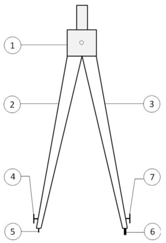
Figure 3.
Structure of a compass.
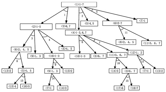
Figure 4.
AND/OR graph of a compass.
As shown in Figure 4, by performing disassembly task 1, subassembly <1> can be disassembled into subassembly <2> and subassembly <3>; then, subassembly <1> is called the parent node of subassembly <2> and subassembly <3>, and subassembly <2> and subassembly <3> are called the child node of subassembly <1>. Subassembly <2> and <3> form an AND relationship. Subassembly <2> can choose to perform disassembly task 3 to obtain subassembly <8> and subassembly <9>, and subassembly <2> can also choose to perform disassembly task 4 to obtain subassembly <5> and subassembly <10>. Disassembly task 3 and disassembly task 4 form an OR relationship, so we can only select one of them to put into the disassembly sequence.
According to the AND/OR graph, we define the following three matrices:
Task relationship matrix: The task relationship matrix is used to describe the conflict relation and precedence relation between the current disassembly task i and other disassembly tasks j. It is defined as
The task relationship matrix of the compass is as follows:
Incidence matrix: The incidence matrix is used to describe the relationship between disassembly tasks and components, which is defined as
Resource use matrix: The resource use matrix is used to describe the use relationship between disassembly task i and disassembly tool r, which is defined as
Taking the compass as an example, there are three kinds of tools needed to disassemble the compass, and we equipped each workstation with these three tools and picked the corresponding tools to perform the disassembly tasks according to the resource use matrix, as follows. According to Table 1, it is known that tool 1 is required to perform task 1 and tool 3 is required to perform task 2.

Table 1.
The task-to-tool relationship for disassembling a compass.
In order to establish a single objective linear disassembly line model, we make the following assumptions:
- (1)
- Matrices A, B and D are known.
- (2)
- The deterioration coefficient of each disassembly tool is known.
- (3)
- The number of workstations is limited.
- (4)
- The working time of each open workstation cannot exceed the cycle time of the workstation.
- (5)
- The switched-on workstation is assigned at least one disassembly task.
- (6)
- The time spent performing the disassembly task is linearly related to the use time of the disassembly tool.
- (7)
- The deterioration cost per unit time and the normal execution time and execution cost of each disassembly task are known.
2.3. Mathematical Model
This part shows the mathematical model of a single product linear disassembly line balancing problem. The notations and decision variables in the mathematical model are defined as follows:
- Sets:
- Indexes:
- Parameters:
- Decision variables:
The following is a mathematical model to describe the problem considered in this work.
The objective function (1) aims to maximize the profits, which is equal to the benefit of the disassembled components minus the workstation cost, tool deterioration cost, and task execution cost. Constraint (2) ensures that each task can only be executed once at most. Constraint (3) ensures that the workstations are turned on in order. Constraint (4) ensures that at most one task can be performed at each location. Constraint (5) indicates that the disassembly task is sequentially assigned to each position of the workstation. Constraint (6) indicates that only one of the two conflicting disassembly tasks can be performed. Constraints (7) and (8) ensure that the open workstation must assign tasks, and the unopened workstation cannot assign tasks. Constraint (9) indicates that the task priority relationship should be satisfied between disassembly tasks. The constraint (10) represents the time each tool has been used before the disassembly task is performed. The constraint (11) represents the actual disassembly time of the task, which are equal to the normal disassembly time of the task plus the deterioration time of the task on the workstation. The constraint (12) represents the deterioration time of the task on the workstation. Constraint (13) indicates that the working time of the workstation cannot exceed the cycle time of the workstation.
3. Proposed Algorithm
Inspired by the “V” shaped flight formation of migratory birds, Duman et al. propose MBO [30]. The “V” formation is a flight mode often used when migratory birds migrate. By flying in the V-formation, birds can save energy and increase flight distance. MBO can find a better solution in a short time by searching the neighborhood of migratory birds and sharing the neighborhood solutions. This search strategy improves the probability of the algorithm searching for the approximate optimal solution and ensures that the solution selected by each individual is not bad. MBO has good convergence and robustness. It can be used to solve various single objective optimization problems. In order to solve the DLBP with tool deterioration, we propose to use DMBO.
3.1. Discrete Migratory Bird Optimizer
In the original MBO, both the leader bird and the follower birds evolved through neighborhood search and sharing neighborhood solutions. After all birds evolved, the leader bird moved to the tail of the left or right queue, and the first follower bird in the left or right queue became a new leader bird, and then proceeded to the next iteration. In this work, we improve the methods of population recombination and replacement of the leader bird, so that the population can approach the optimal solution faster. In addition, we design three mutation strategies to increase the diversity of the population in order to avoid the algorithm falling into local optimization.
The main content of DMBO is individual evolution. After birds in the population are arranged into the V shape, each bird can generate some neighborhood solutions through crossover operators and mutation operators and select a better individual from the neighborhood solutions to replace itself. Unused neighborhood solutions are shared with the next bird to help it evolve. The neighborhood solution set of the leader bird is expressed as , and the neighborhood solution sets of the left and right following birds are expressed as and . The detailed steps of DMBO are shown in Algorithm 1.
| Algorithm 1: Discrete migratory bird optimizer |
|
- (a)
- Population initialization: Based on the population size n, n feasible solutions are randomly generated, and one feasible solution represents a migratory bird.
- (b)
- Construct V formation queue: Select a stronger individual in the population as the leader bird, and the other birds are divided to the left and right sides to form a V shape in turn, and the left and right queues are represented as and .
- (c)
- The evolution of the leader: The leader bird generates several neighborhood solutions according to the evolutionary strategy, then puts the neighborhood into , and compares the individuals in with the leader bird. If an individual better than the leader bird is found in , the leader bird is replaced; if it is not found, the leader bird is not replaced. Finally, the unused neighborhood solution is passed to the followers.
- (d)
- The evolution of the follower: First, the follower birds generate neighborhood solutions according to the evolutionary strategy, then we put the neighborhood solutions and the solutions passed by the previous birds into or . If the individual in / is better than the current follower bird, the follower is replaced. The detailed steps of individual evolution are shown in Algorithm 2.
- (e)
- Recombination of population and replacement of the leader bird: When the set number of cycles has been reached, all migratory birds in the population have evolved, and then the initial population and the new individuals are aggregated to form a new set B. In order to make the population move closer to the optimal solution faster, we mutate the initial population and add it to set B. Then, we traverse the individuals in the set, select the best n individuals to build a new population, select the best one from the n individuals to be the leader bird, and assign the remaining individuals to the left and right in turn. Furthermore, we put the best one in the external archive X.
The algorithm terminates when the preset maximum iterations are reached.
| Algorithm 2: Individual evolution |
|
3.2. Encoding and Decoding
Based on the characteristics of DLBP with tool deterioration, we want to obtain a set of disassembly sequences for the EOL products and assign them reasonably to several workstations in a disassembly line according to our disassembly goals. To more clearly describe the problem under study, we use encoding and decoding to interpret a solution.
We design a two-stage encoding method that defines an integer string to represent a solution. represents a sequence of disassembly tasks, and represents the corresponding workstation sequence of the disassembly tasks in . Take a solution of the compass as an example, as shown in Figure 5. When a new individual is generated, a disassembly task sequence is randomly generated, and then the task sequence is adjusted according to the conflict and precedence relation matrices of the disassembly task to make it a feasible task sequence.

Figure 5.
Encoding example.
In the decoding process, each task in the sequence of feasible tasks is assigned to the workstation in turn and satisfies the cycle time constraints of the workstation. When assigning a task, we calculate whether the total disassembly time of all disassembly tasks on the current workstation exceed the workstation’s cycle time after assigning the task to the current workstation. If the total disassembly time exceeds the cycle time of the workstation after assigning the task, the task is assigned to the next workstation. If the total disassembly time does not exceed the workstation’s cycle time after assigning the task, we randomly assign the task to the current or next workstation. The decoding diagram is shown in Figure 6. In summary, the disassembly task sequence can be decoded to obtain a specific solution, after which we can calculate and evaluate the target function value of the solution.
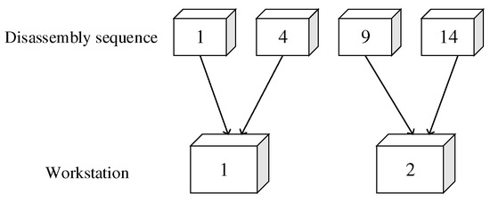
Figure 6.
Assign tasks to workstations.
3.3. Evolution of Leader and Followers
In DMBO, after population initialization is complete, for the individuals in the population to evolve in the direction we want, we need to generate some new individuals to update the population. In this study, the precedence preserving crossover (PPX) operator and three mutation operators are designed to help the leader and follower birds to evolve.
PPX operator enables individuals to maintain precedence and conflict constraints after crossover. As Figure 7 shows, the specific steps for PPX are as follows:
- (a)
- Traverse the V-shaped queue formed by the migratory bird population, and select the current migratory bird and its next migratory bird as parent 1 and parent 2, respectively.
- (b)
- Randomly generate a mask represented by a binary number, and parent 1 and parent 2 generate new individuals according to this mask. The 0 in this mask means to obtain the disassembly task from parent 1, and the 1 means to obtain the disassembly task from parent 2. If the acquired task already exists in the new individual, we need to skip the current task and obtain the next one from the parent.
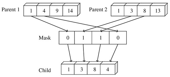
Figure 7.
Process of crossover.
In order to increase the diversity of solutions, we need to conduct mutation operations on new individuals. The mutation operators we designed are as follows:
- (a)
- Task sequence variation: Under the premise of not exceeding the total number of tasks in the case, appropriately add 1 to 3 tasks randomly after the individual task sequence. As shown in Figure 8, two tasks are randomly added after the individual task sequence to make the task sequence longer. This mutation strategy can solve the problem of shortening the individual task sequence after the crossover operation.
- (b)
- Location variation: Starting from the second task in the task sequence, randomly select a task, find out the location of the superior task and subordinate task of the task according to the priority relationship of the task, and randomly select a location between the two locations to insert the task. As shown in Figure 9, in the current task sequence, select task 14 randomly. Its superior task is task 1, and its subordinate task is task 9. Then, insert task 14 in a randomly selected position between task 1 and task 9.
- (c)
- Workstation variation: Randomly select a workstation in the current solution, assign the first task on the workstation to the previous workstation, or assign the last task on the workstation to the next workstation. As shown in Figure 10, the second workstation is randomly selected, and the first task 14 on the second workstation is assigned to workstation 1.
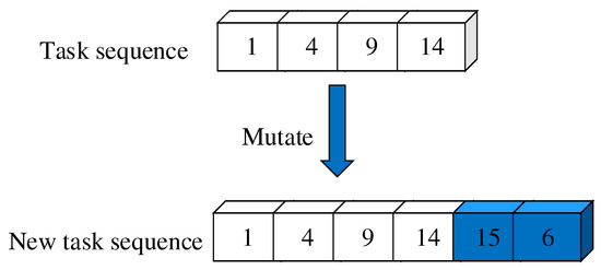
Figure 8.
Process of task sequence variation.
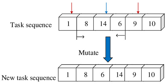
Figure 9.
Process of location variation.
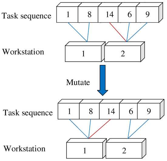
Figure 10.
Process of workstation variation.
4. Experimental Results
4.1. Test Instances
DMBO is implemented on IntelliJ IDEA 2020.3.3 x64 and runs under the Jmetal framework. The mathematical model is verified in IBM ILOG CPLEX Optimization Studio. The operating environment is Windows 10, and the CPU is AMD a6-9210 Radeon r4,5 computer cores 2C + 3G 2.40 GHz.
In order to make the experimental results more reliable and comprehensive, we select six disassembly cases of different scales for testing, among which the ballpoint pen [35] (see Figure 11), washing machine [36] (see Figure 12 and Figure 13) and compass [37] (see Figure 3) are small-scale cases; the refrigerator [38] (see Figure 14) and radio [35] (see Figure 15) are medium-scale cases; and the hammer drill [39] (see Figure 16) is a large-scale case. The details of the six cases are shown in Table 2.

Figure 11.
Disassembly diagram of a ballpoint pen.
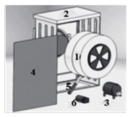
Figure 12.
Disassembly diagram of a washing machine.
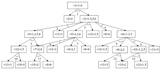
Figure 13.
AND/OR graph of a washing machine.

Figure 14.
Disassembly precedence graph of the refrigerator.
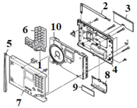
Figure 15.
Structure of a radio.
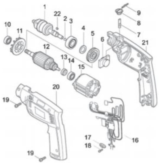
Figure 16.
Structure of a hammer drill.

Table 2.
Test cases.
Before starting the experiment, we need to set the parameters of each case. Take the radio as an example. Its parameter settings are shown in Table 3. C represents the deterioration cost per unit time. The total deterioration cost can be obtained by multiplying C by the total deterioration time. represents the fixed cost of opening the workstation. Multiply by the number of workstations opened to obtain the total cost of workstations opened. The values of W and K are set based on the scale of the case. R is set based on the kind of tools needed to disassemble the product. represents the degree of tool deterioration. The higher the value of , the longer it takes to execute task i with this tool. indicates the normal disassembly time of task i without considering tool deterioration. represents the profit of component n. Our goal is to disassemble the components with high profit as much as possible. represents the disassembly cost of task i. For each task executed, we add its disassembly cost to the total cost. T in Table 2 represents the cycle time of the workstation, which is set according to the scale of the case.

Table 3.
Parameter settings for the radio.
4.2. Comparative Analysis of DMBO and CPLEX Results
In order to verify the correctness of the mathematical model and the performance of the algorithm, we use CPLEX and DMBO to solve six test cases separately [40]. The results of six cases solved based on CPLEX are shown in Table 4. We take the solution of the washing machine as an example. The meaning of the disassembly sequence is that task 1, task 4, and task 8 are assigned to the first workstation, and task 12 is assigned to the second workstation, the total profit obtained by the disassembly assignment is 1155. When small-scale cases such as washing machines and ball pens are solved by CPLEX, the optimal solution can be accurately obtained in a very short time. For medium-scale cases such as the radio, it takes a long time to solve with CPLEX, which is significantly increased compared with small-scale cases, but it can also find the optimal solution in a certain time. When using CPLEX to solve large-scale cases such as hammer drills, it is still inefficient to obtain a feasible solution after running for five hours. In this article, we use “-” to indicate that no results have been obtained. Therefore, it can be concluded that the size of the experimental case has a great impact on the efficiency of CPLEX.

Table 4.
Results of solving the instances with CPLEX.
The results of six cases solved based on DMBO are shown in Table 5. For the small- and medium-sized cases, DMBO achieved the same optimal solution as CPLEX, indicating the correctness and effectiveness of the DMBO. In the case of the hammer drill, CPLEX failed to obtain a feasible solution within 5 h, while DMBO converged to a feasible solution within seconds, demonstrating the excellent search capability of DMBO. The computation time of DMBO does not show significant differences across different case sizes, implying that the size of the experimental cases has little impact on the efficiency of DMBO.

Table 5.
Results of solving the instances with DMBO.
In Table 6, we study the optimal values and computation times obtained for the six cases based on CPLEX and DMBO, through which it is known that, for the same case, DMBO takes significantly less time to obtain the optimal solution than CPLEX, and DMBO can achieve as good or better solutions than CPLEX.

Table 6.
Comparison of results between DMBO and CPLEX.
4.3. Analysis of DMBO Performance
Figure 17 shows the initial and optimal solutions for the radio disassembly. We use cyan to indicate that the task uses tool 1, blue to indicate that the task uses tool 2, and orange to indicate that the task uses tool 3. In the initial solution, there are two tasks on workstation 1 and workstation 2 that use the same tool. Due to the deterioration effect of the tool, the disassembly time of workstation 1 and workstation 2 is extended. In the optimal solution obtained by DMBO, tasks using the same tool are assigned to different workstations to reduce the impact of tool deterioration. Table 7 lists the detailed data of the initial solution and the optimal solution. From this table, we can see that in the initial solution, the deterioration effect occurred on workstations 1 and 2, resulting in a total extension of the task execution time by 22.9 and a deterioration cost of 45.8. After the optimization of the algorithm, the impact of tool deterioration is avoided, and the profit of the final solution is increased by 2.51%. This shows that DMBO has good optimization performance.
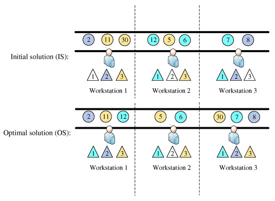
Figure 17.
Initial solution and optimal solution of radio.

Table 7.
Comparison between the initial solution (IS) and optimal solution (OS).
In many existing studies on DLBP, the impact of deterioration effect on disassembly profit in disassembly lines is not considered. When solving the optimal solution without considering the deterioration effect of disassembly tools, we obtain the disassembly solution as shown in Figure 18. From the figure, we can see that there are multiple tasks using the same tool on workstation 1 and workstation 2. However, in the actual disassembly process, the deterioration effect is inevitable. If we disassemble the radio according to the solution in Figure 18, the execution time of tasks 19, 27, and 29 will be extended. Table 8 lists the comparison between the two solutions with or without tool deterioration. From this table, we can see that the execution time of the tasks is prolonged by 55.65 and the deterioration cost is increased by 111.3 when the deterioration of the tool is not considered. However, if we consider the deterioration effect of tools and avoid the impact of tool deterioration on disassembly time and cost, the disassembly profit of radio will increase by 5.49%. Therefore, it is necessary to consider the impact of tool deterioration in DLBP.
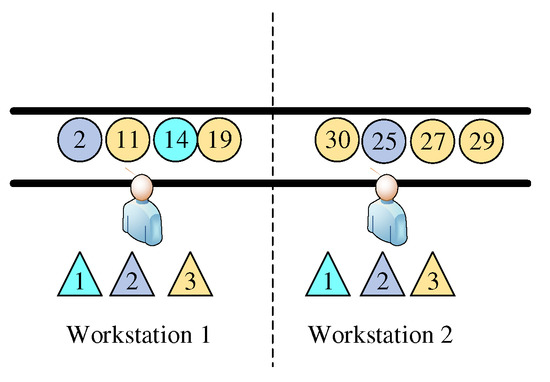
Figure 18.
Optimal solution of radio without considering tool deterioration (OSWT).

Table 8.
Comparison of solutions with (OSWT) and without (OS) tool deterioration.
4.4. Comparison between DMBO and Other Algorithms
In order to check the performance of DMBO in solving optimization problems, we also use discrete fruit fly optimization algorithm (DFOA) [41], a discrete whale optimization algorithm (DWOA) [42], and a salp swarm algorithm (SSA) [43] to solve the problems in this study. DFOA is easy to understand and implement, with low computational complexity and strong local search capabilities. DWOA is a swarm intelligence optimization algorithm that mimics the behavior of humpback whales during hunting. It has the characteristics of fewer parameters and fast convergence speed. SSA has low complexity, strong flexibility and basically does not require parameter settings, making it have good application prospects in various optimization fields. Under the condition of 400 iterations and 100 population sizes, 20 experiments are carried out, the optimal value of each generation is recorded in each experiment, and then the average value of each generation is calculated. Take the radio as an example. Its iterative process is shown in Figure 19. From the iteration chart, it can be observed that DMBO exhibits strong global search capability. Compared to the other three algorithms, DMBO converges faster and is able to find better solutions in fewer iterations.
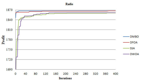
Figure 19.
Iterative comparison of four algorithms.
In addition, we also sorted out the optimal value, the worst value and the average value of each algorithm in 20 experiments, as shown in Table 9. From this table, we can find that with the increase in the case size, the quality of the solution of DMBO is better and the performance of DMBO remains stable.

Table 9.
Experimental results of stability test.
5. Conclusions
In this work, considering the fact that disassembly tools deteriorate in functions when they are being used, a single product disassembly model with the goal of maximal profit is proposed, which attempts to assign tasks that use the same tool to different workstations. CPLEX is used to validate the correctness of the model. The results of a series of experiments show that the proposed DMBO algorithm has a good performance in solving DLBP and is superior to DFOA and other algorithms. The comparison of DMBO with CPLEX on their computation time to achieve optimal solution reveals that DMBO is more efficient. For small-scale cases, DMBO runs faster and can obtain solutions that are as good as CPLEX. For some large-scale cases, CPLEX cannot find the optimal solution. However, DMBO can find a feasible solution in a short time. Therefore, DMBO can be used to solve the disassembly of small-scale cases such as ballpoint pens and washing machines, as well as medium-scale and large-scale cases such as radios and hammer drills.
Our next step is to apply DMBO to solve multi-objective disassembly balancing problems on different types of disassembly layouts, such as U-shaped disassembly lines and parallel disassembly lines. We will also explore the tool feasibility on workstations and the influence of tool change, as well as consider uncertainty factors in EOL products.
Author Contributions
Conceptualization, X.G. and L.Q.; methodology, S.Q.; validation, J.W. (Jiaxin Wang) writing—original draft preparation, S.Q.; writing—review and editing, J.W. (Jiacun Wang); visualization, Y.F.; supervision, L.Q. All authors have read and agreed to the published version of the manuscript.
Funding
This work is supported in part by NSFC under Grant 61903229, in part by Liaoning Revitalization Talents Program under Grant XLYC1907166, in part by the Natural Science Foundation of Shandong Province under Grant ZR2019BF004, and in part by Archival Science and Technology Project of Liaoning Province under Grant 2021-B-004.
Data Availability Statement
The data presented in this study are available on request from the corresponding author.
Conflicts of Interest
The authors declare no conflicts of interest.
References
- Zai, A.; Sm, B.; Fs, C. Robotic disassembly line balancing problem: A mathematical model and ant colony optimization approach. Appl. Math. Model. 2020, 86, 335–348. [Google Scholar]
- Bahubalendruni, M.R.; Varupala, V.P. Disassembly sequence planning for safe disposal of end-of-life waste electric and electronic equipment. Natl. Acad. Sci. Lett. 2021, 44, 243–247. [Google Scholar] [CrossRef]
- Feng, Y.; Gao, Y.; Tian, G.; Li, Z.; Hu, H.; Zheng, H. Flexible process planning and end-of-life decision-making for product recovery optimization based on hybrid disassembly. IEEE Trans. Autom. Sci. Eng. 2018, 16, 311–326. [Google Scholar] [CrossRef]
- Zhu, Q.; Tang, H.; Huang, J.; Hou, Y. Task Scheduling for Multi-Cloud Computing Subject to Security and Reliability Constraints. IEEE/CAA J. Autom. Sin. 2021, 8, 848–865. [Google Scholar] [CrossRef]
- Anil Kumar, G.; Bahubalendruni, M.R.; Prasad, V.; Sankaranarayanasamy, K. A multi-layered disassembly sequence planning method to support decision making in de-manufacturing. Sādhanā 2021, 46, 102. [Google Scholar] [CrossRef]
- Zhou, Z.; Liu, J.; Pham, D.T.; Xu, W.; Ramirez, F.J.; Ji, C.; Liu, Q. Disassembly sequence planning: Recent developments and future trends. Proc. Inst. Mech. Eng. Part B J. Eng. Manuf. 2019, 233, 1450–1471. [Google Scholar] [CrossRef]
- Gulivindala, A.K.; Bahubalendruni, M.; Chandrasekar, R.; Ahmed, E.; Abidi, M.H.; Al-Ahmari, A. Automated disassembly sequence prediction for industry 4.0 using enhanced genetic algorithm. Comput. Mater. Contin. 2021, 69, 2531–2548. [Google Scholar] [CrossRef]
- Gungor, A.; Gupta, S.M. A solution approach to the disassembly line balancing problem in the presence of task failures. Int. J. Prod. Res. 2001, 39, 1427–1467. [Google Scholar] [CrossRef]
- McGovern, S.M.; Gupta, S.M. A balancing method and genetic algorithm for disassembly line balancing. Eur. J. Oper. Res. 2007, 179, 692–708. [Google Scholar] [CrossRef]
- Kalayci, C.B.; Gupta, S.M. A particle swarm optimization algorithm with neighborhood-based mutation for sequence-dependent disassembly line balancing problem. Int. J. Adv. Manuf. Technol. 2013, 69, 197–209. [Google Scholar] [CrossRef]
- Tuncel, E.; Zeid, A.; Kamarthi, S. Solving large scale disassembly line balancing problem with uncertainty using reinforcement learning. J. Intell. Manuf. 2012, 25, 647–659. [Google Scholar] [CrossRef]
- Liu, J.; Wang, S. Balancing Disassembly Line in Product Recovery to Promote the Coordinated Development of Economy and Environment. Sustainability 2017, 9, 309. [Google Scholar] [CrossRef]
- Hu, B.; Feng, Y.; Zheng, H.; Tan, J. Sequence planning for selective disassembly aiming at reducing energy consumption using a constraints relation graph and improved ant colony optimization algorithm. Energies 2018, 11, 2106. [Google Scholar] [CrossRef]
- Guo, X.; Wei, T.; Wang, J.; Liu, S.; Qin, S.; Qi, L. Multiobjective U-shaped disassembly line balancing problem considering human fatigue index and an efficient solution. IEEE Trans. Comput. Soc. Syst. 2023, 10, 2061–2073. [Google Scholar] [CrossRef]
- Liu, C.; Xiong, C. Single machine resource allocation scheduling problems with deterioration effect and general positional effect. Math. Biosci. Eng. 2021, 18, 2562–2578. [Google Scholar] [CrossRef] [PubMed]
- Kalaki Juybari, J.; Kalaki Juybari, S.; Hasanzadeh, R. Parallel machines scheduling with time-dependent deterioration, using meta-heuristic algorithms. SN Appl. Sci. 2021, 3, 333. [Google Scholar] [CrossRef]
- Mir, M.S.S.; Rezaeian, J.; Mohamadian, H. Scheduling parallel machine problem under general effects of deterioration and learning with past-sequence-dependent setup time: Heuristic and meta-heuristic approaches. Soft Comput. 2020, 24, 1335–1355. [Google Scholar]
- Gupta, J.N.; Gupta, S.K. Single facility scheduling with nonlinear processing times. Comput. Ind. Eng. 1988, 14, 387–393. [Google Scholar] [CrossRef]
- Ng, C.T.; Cheng, T.E.; Bachman, A.; Janiak, A. Three scheduling problems with deteriorating jobs to minimize the total completion time. Inf. Process. Lett. 2002, 81, 327–333. [Google Scholar] [CrossRef]
- Cheng, M.; Sun, S. Two scheduling problems in group technology with deteriorating jobs. Appl. Math. J. Chin. Univ. 2005, 20, 225–234. [Google Scholar]
- Toksarı, M.D.; Güner, E. Minimizing the earliness/tardiness costs on parallel machine with learning effects and deteriorating jobs: A mixed nonlinear integer programming approach. Int. J. Adv. Manuf. Technol. 2008, 38, 801–808. [Google Scholar] [CrossRef]
- Wang, J.; Ji, P.; Cheng, T.C.E.; Wang, D. Minimizing makespan in a two-machine flow shop with effects of deterioration and learning. Optim. Lett. 2011, 6, 1393–1409. [Google Scholar] [CrossRef]
- Behnamian, J. Scheduling and worker assignment problems on hybrid flowshop with cost-related objective function. Int. J. Adv. Manuf. Technol. 2014, 74, 267–283. [Google Scholar] [CrossRef]
- Kouka, S.; Makhadmeh, S.N.; Al-Betar, M.A.; Dalbah, L.M.; Nachouki, M. Recent Applications and Advances of Migrating Birds Optimization. Arch. Comput. Methods Eng. 2023, 31, 243–262. [Google Scholar] [CrossRef]
- Qin, G.; Guo, X.; Liu, S.; Qi, L.; Zhao, J.; Zhao, Z.; Tang, Y. Multi-objective Discrete Migrating Birds Optimizer Solving Multiple-product Partial U-shaped Disassembly Line Balancing Problem. In Proceedings of the 2021 IEEE 29th Mediterranean Conference on Control and Automation (MED), Puglia, Italy, 22–25 June 2021; pp. 59–64. [Google Scholar]
- Gad, A.G.; Houssein, E.H.; Zhou, M.; Suganthan, P.N.; Wazery, Y.M. Damping-assisted evolutionary swarm intelligence for industrial iot task scheduling in cloud computing. IEEE Internet Things J. 2023, 11, 1698–1710. [Google Scholar] [CrossRef]
- Fu, Y.; Ma, X.; Gao, K.; Li, Z.; Dong, H. Multi-Objective Home Health Care Routing and Scheduling With Sharing Service via a Problem-Specific Knowledge-Based Artificial Bee Colony Algorithm. IEEE Trans. Intell. Transp. Syst. 2023. [Google Scholar] [CrossRef]
- Ulker, E.; Tongur, V. Migrating birds optimization (MBO) algorithm to solve knapsack problem. Procedia Comput. Sci. 2017, 111, 71–76. [Google Scholar] [CrossRef]
- Makas, H.; Yumuşak, N. System identification by using migrating birds optimization algorithm: A comparative performance analysis. Turk. J. Electr. Eng. Comput. Sci. 2016, 24, 1879–1900. [Google Scholar] [CrossRef]
- Duman, E.; Uysal, M.; Alkaya, A.F. Migrating birds optimization: A new metaheuristic approach and its performance on quadratic assignment problem. Inf. Sci. 2012, 217, 65–77. [Google Scholar] [CrossRef]
- Kalayci, C.B.; Shaaban, S.; Gupta, S.M. Ant colony optimization for sequence-dependent disassembly line balancing problem. J. Manuf. Technol. Manag. 2013, 24, 413–427. [Google Scholar] [CrossRef]
- Wang, J.; Guo, X.; Wang, J.; Qin, S.; Qi, L.; Tang, Y. Discrete Migratory Bird Optimizer for Disassembly Line Balancing Problem Considering Tool Deterioration. In Proceedings of the 2022 IEEE International Conference on Networking, Sensing and Control (ICNSC), Shanghai, China, 15–18 December 2022; pp. 1–6. [Google Scholar]
- Fu, Y.; Zhou, M.; Guo, X.; Qi, L. Scheduling dual-objective stochastic hybrid flow shop with deteriorating jobs via bi-population evolutionary algorithm. IEEE Trans. Syst. Man Cybern. Syst. 2019, 50, 5037–5048. [Google Scholar] [CrossRef]
- Wang, J. Patient flow modeling and optimal staffing for emergency departments: A Petri net approach. IEEE Trans. Comput. Soc. Syst. 2023, 10, 2022–2032. [Google Scholar] [CrossRef]
- Lu, Q.; Ren, Y.; Jin, H.; Meng, L.; Li, L.; Zhang, C.; Sutherland, J.W. A hybrid metaheuristic algorithm for a profit-oriented and energy-efficient disassembly sequencing problem. Robot. Comput.-Integr. Manuf. 2020, 61, 101828. [Google Scholar] [CrossRef]
- Zitzler, E.; Thiele, L.; Laumanns, M.; Fonseca, C.M.; Da Fonseca, V.G. Performance assessment of multiobjective optimizers: An analysis and review. IEEE Trans. Evol. Comput. 2003, 7, 117–132. [Google Scholar] [CrossRef]
- Bentaha, M.L.; Battaïa, O.; Dolgui, A. L-shaped algorithm for stochastic disassembly line balancing problem. IFAC Proc. Vol. 2013, 46, 407–411. [Google Scholar] [CrossRef]
- Zhu, L.; Zhang, Z.; Guan, C. Multi-objective partial parallel disassembly line balancing problem using hybrid group neighbourhood search algorithm. J. Manuf. Syst. 2020, 56, 252–269. [Google Scholar] [CrossRef]
- Pistolesi, F.; Lazzerini, B.; Dalle Mura, M.; Dini, G. EMOGA: A hybrid genetic algorithm with extremal optimization core for multiobjective disassembly line balancing. IEEE Trans. Ind. Inform. 2017, 14, 1089–1098. [Google Scholar] [CrossRef]
- Ma, X.; Fu, Y.; Gao, K.; Zhu, L.; Sadollah, A. A multi-objective scheduling and routing problem for home health care services via brain storm optimization. Complex Syst. Model. Simul. 2023, 3, 32–46. [Google Scholar] [CrossRef]
- Han, M. A V2G scheduling strategy based on the fruit fly optimization algorithm. J. Phys. Conf. Ser. 2021, 1952, 042063. [Google Scholar] [CrossRef]
- Li, Y.; He, Y.; Liu, X.; Guo, X.; Li, Z. A novel discrete whale optimization algorithm for solving knapsack problems. Appl. Intell. 2020, 50, 3350–3366. [Google Scholar] [CrossRef]
- Chamchuen, S.; Siritaratiwat, A.; Fuangfoo, P.; Suthisopapan, P.; Khunkitti, P. Adaptive Salp Swarm Algorithm as Optimal Feature Selection for Power Quality Disturbance Classification. Appl. Sci. 2021, 11, 5670. [Google Scholar] [CrossRef]
Disclaimer/Publisher’s Note: The statements, opinions and data contained in all publications are solely those of the individual author(s) and contributor(s) and not of MDPI and/or the editor(s). MDPI and/or the editor(s) disclaim responsibility for any injury to people or property resulting from any ideas, methods, instructions or products referred to in the content. |
© 2024 by the authors. Licensee MDPI, Basel, Switzerland. This article is an open access article distributed under the terms and conditions of the Creative Commons Attribution (CC BY) license (https://creativecommons.org/licenses/by/4.0/).