Article

A Formalization of Multilabel Classification in Terms of Lattice Theory and Information Theory: Concerning Datasets

by
Francisco J. Valverde-Albacete
1,*,† and
Carmen Peláez-Moreno
2,†
1
Department of Signal Theory and Communications, Telematic Systems and Computation, Universidad Rey Juan Carlos, 28942 Fuenlabrada, Madrid, Spain
2
Department of Signal Theory and Communications, Universidad Carlos III de Madrid, 28911 Leganés, Madrid, Spain
*
Author to whom correspondence should be addressed.
These authors contributed equally to this work.
Mathematics 2024, 12(2), 346; https://doi.org/10.3390/math12020346
Submission received: 28 November 2023 / Revised: 29 December 2023 / Accepted: 15 January 2024 / Published: 21 January 2024
(This article belongs to the Special Issue Applications of Mathematics in Neural Networks and Machine Learning)

Abstract

:
Multilabel classification is a recently conceptualized task in machine learning. Contrary to most of the research that has so far focused on classification machinery, we take a data-centric approach and provide an integrative framework that blends qualitative and quantitative descriptions of multilabel data sources. By combining lattice theory, in the form of formal concept analysis, and entropy triangles, obtained from information theory, we explain from first principles the fundamental issues of multilabel datasets such as the dependencies of the labels, their imbalances, or the effects of the presence of hapaxes. This allows us to provide guidelines for resampling and new data collection and their relationship with broad modelling approaches. We have empirically validated our framework using 56 open datasets, challenging previous characterizations that prove that our formalization brings useful insights into the task of multilabel classification. Further work will consider the extension of this formalization to understand the relationship between the data sources, the classification methods, and ways to assess their performance.

1. Introduction

Multilabel classification (MLC) is a relatively recently-formalized task in machine learning [1] with applications in text categorization [2], medicine [3], or remote sensing [4], among others. A recent, extensive evaluation provides a catalogue of technical issues and concerns in solving the MLC task [5], while more dated tutorials explain the progress in methods and concerns [6,7] or with special emphasis on software tools [8]. Finally, Ref. [9] sets MLC in the broader task of multi-target prediction.

1.1. Formalization

Let L be a set of l = | L | labels any of whose subsets is a labelset. We may assign to each of the labels a certain “meaning” but this is outside of this mathematical model for now. Consider a space Y 2 l , whose elements are also called labelsets y Y via the isomorphism with their characteristic vectors. Suppose that we can only access the result of an observation process on the labelsets in terms of visible instances, observations, or feature vectors in a feature space X R m . Then, the multilabel classification problem is to tag any (feature) vector x X with a labelset y Y .
Note that the problems of supervised machine classification or regression in Statistical Machine Learning (SML) can be solved with predictive inference [10]. This is a very general metaphor for statistical investigation of random vectors: consider a categorical random variable Y P Y . Suppose that this variable is hidden and we can only access random vectors X ¯ P X ¯ , acting as observations x X ¯ of the y Y . In predictive inference we want to recover y Y by applying an inference function to a new observation x X ¯ .
Metaphor 1 
(Predictive Inference is Transmitting Information through a Channel). Figure 1 depicts a communication channel where:
  • Variable Y represents a partially hidden source of information;
  • The random vector X ¯ represents an encoding of that partially inaccessible information in the form favoured by an (unknown) observation process;
  • The recovered Y ^ is the result of decoding the information in x .
Figure 1. Basic scheme for predictive inference as a communication channel. S = Source and P = Presentation , standing for the origin and the purpose or destination, respectively, of the data to be inferred.
Mathematics 12 00346 g001
We use here “metaphor” in the sense of Metaphor Theory [11] as applied to Mathematics whereby conceptual metaphors preserve inferences and calculations encode those inferences [12]. This metaphor suggests that MLC datasets are actually partially observed multivariate binary sources of information, and that the MLC task should be assessed as a process that transports this information to a destination or target for further (unspecified) use.
Since MLC is a supervised task, we describe in Figure 2 its solution using predictive inference (compare with the solution proposed in Section 3.4).
The engineering part of SML consists, then, in filling the details of this pseudo-algorithm. In this paper, however, we propose a new mathematical framework to improve the mathematical models of SML to better guide and help in the filling of those details and in particular, it will become apparent why a first step is missing and how should it be completed.

1.2. Some Fundamental Issues in MLC

1.2.1. Classifier Design for MLC

Since the MLC task can be considered a strict generalization of the binary and multiclass classification tasks in that instances may have more than one label (class) assigned to them, most of the techniques for classifier design have been imported therefrom: performance measure selection, data preparation, and classifier evaluation have required extensions to cater for the peculiarities of MLC.
In particular, since the theory of statistical machine learning is traditionally grounded on the binary or mutually-exclusive labelling cases, dealing with label sets poses a challenge usually solved by means of problem transformation. The extreme cases of these transformations are [13]:
  • Binary relevance (BR) [14], a problem transformation method that learns L binary classifiers—one for each different label in L —and then transforms the original data set into L data sets D l j ; j = 1 L that contain all examples of the original data set, labelled positively if the label set of the original example contained l j and negatively otherwise. To classify a new instance BR outputs the union of the labels l j that are positively predicted by the L classifiers.
  • Classifier Chains (CC) [15,16], a transformation method that orders the labels by their decreasing predictive power on later labels and trains classifiers for each of these in order: all previous labels are used as inputs to predict later labels. Other hierarchical approaches, use lattice-based methods to define the labelset hierarchy, for example [17].
  • Label Powerset (LP) [1], a simple but effective problem transformation method that considers each unique set of labels in a multilabel training set as one of the classes of a new single-label classification task. Given a new instance, the single-label classifier of LP outputs the most probable class, which is actually a set of labels. Bad initial performance results suggested the Rakel [13] variant.
In this paper, we concentrate on analysing the datasets that pre-form the possible solutions to the MLC problem, rather than the solutions themselves. Hence, issues that are nuclear in traditional MLC concerns—e.g., algorithm adaptation, stacking, etc.—play no part herein but will be re-taken in future work (see Section 3.5).

1.2.2. Modelling Label Dependencies

It was early on hinted that performance measures presuppose one model of dependence or another [18]; hence, explicit modelling of dependences quickly became an issue to understand the task. Few solutions to the MLC try to model explicitly such dependencies—a notable exception to this is CC [19] (Chap. 7) and its derivatives, consistently showing better performance results than LP but not BR.
Note that, from a purely theoretical machine learning perspective, while for BR it is important that labels be actually independent, for CC it is important to order the labels in decreasing dependence order. Likewise, it is important to reduce the cardinality of Y for LP and that the appearance of labelsets be balanced.
Actually, whether one method will outperform the other is presently believed to correlate with the degree of dependence on labels among themselves: if labels are mostly non-dependent, then the BR method is superior to LP, while the contrary is expected to hold when dependence between labels is commonplace [13,19]. Recent theoretical work supports this hypothesis [5].

1.2.3. Label Imbalance in MLC Datasets

Here, we take “label imbalance” as the deviation from the equiprobability distribution on a label, whether it be binary or multiclass. Label imbalance seems to impinge on the results of MLC rather heavily. In the single label classification case, extreme imbalance makes the task resemble a detection task, rather than a classification task, whereas, arguably, balancedness makes it harder for any classification technique to improve its performance by concentrating in majority classes [20].
In MLC these phenomena are compounded with the appearance of labelsets that are rare combinations of labels. In the domain of language modelling, rare sequences of particular words are called hapaxes (apparently from ancient Gr. hapax legomenon, “single word”). Since in MLC labels are mostly textual, and labelsets are typically represented in a conventional ordering of the labels, the category is applicable too.
A review of the methods applicable to imbalanced MLC stresses the importance of taking into account this phenomenon but focuses on the taxonomies of data resampling and classifier adaptation methods [21]. However, we know of no study that provides a framework to characterise the datasets in this regard, or guidelines to deal with the phenomenon, except for early attempts to heuristically measure the imbalanceness using the so-called imbalance ratio [22] employed for example in [2,23]. Yet, label independence may allow us to split up a MLC task into several independent ones ameliorating the problem of labelsets that are hapaxes. This is one more reason to detect or model label independence correctly.

1.2.4. Types of MLC Datasets

In our opinion, the consideration of the intrinsic characteristics of the features as lending themselves to MLC has not been properly explored in traditional MLC reviews. For instance, a recent—otherwise very thorough—strategy- and classifier-based analysis of MLC architectures [5], deals with dataset characteristics by describing what (media) modality they refer to and, perhaps, making a statistical analysis of label and labelset measures. It should be clarified, by the way, that multi-modality datasets are being called multi-view in recent years which brings to the table all the traditional concerns of multi-modality: fusion, decision, etc. [24]
In another paper, the same group of authors carry out a more extensive meta-exploration of a set of MLC datasets whose main results is a dataset clustering with an overall structure of eight different clusters [25]. Some measurements on these datasets relevant to our studies are collected in Table 1.
For each dataset we collected: | B L ( G , L , I ) | the size of the lattice of intents of the labelling context (see Section 3.1.1), d the number of distinct labelsets, | L | the number of labels, n that of observations, and | F | that of features.
A facet of this exploration that is so far missing is the consideration of the structure of the set of labelsets. We try to prove in Section 3.1 that such structure, indeed an order lattice [28], is crucial to understand the nature of the dataset in question. It may also be relevant for strategy selection (see Section 3.5).

1.3. Research Goals

In trying to solve an instance of an MLC task two questions are immediately apparent:
  • What is an “easy” or “hard” dataset to carry out MLC on?
    This in turn involves answering two questions:
    (a)
    How “difficult” is the set of labels to learn of its own?
    (b)
    How “difficult” is it to predict the labels from the observations?
  • Given the answers to the previous question, what is the most appropriate way to address the MLC problem?
Most works on the MLC task address the second question following the guidelines stated in Section 1.2—see, e.g., ref. [8] and references therein.
However, a few works try to answer question number 1. Perhaps the most developed set of methods at present is meta-analysis, e.g., as carried by [25,29,30], where insights obtained in experimental conditions are put in relation to dataset descriptions. This is a post hoc, indirect method to measure features of MLC datasets that make them “difficult” or “easy”.
In this paper, we want to put forward a mathematical modelling approach based on lattice theory [28,31] and information theory [32] to solve problem 1 above, that is, to ascertain from first principles how difficult an MLC task is. For this purpose we exploit the model or metaphor of supervised ML tasks as information communication channels.
Our use of “information” is not the usual and trite “intelligence is the adequate use of information”, but the tangible application of three measures of information as related by a balance equation that allows us to explore the compromise between independence, correlation, and maximal randomness in stochastic, binary sources of information [33].
We claim that MLC datasets can be effectively modelled as special formal contexts in the framework of formal concept analysis [34]. Specifically, we look through the lens of information theory at the encoding of information in scales as used in data modelling to transform non-binary into binary data.

1.4. Reading Guide

For that purpose we first discuss in full the Classification is Information Transmission metaphor in Section 2.1. This sets the backdrop to introduce methods to measure the information content of sources both quantitatively and qualitatively in Section 2.2 and Section 2.3, respectively.
We describe our results in Section 3. First we carry out an analysis of the information content of multilabel sources in Section 3.1, starting with a theoretical development for sources that resemble multiclass sources in the context of prototypical degrees of dependency between labels (Section 3.1.1), following with a data-driven analysis of insights obtained from qualitative (Section 3.1.2) and quantitative (Section 3.1.3) information in MLC datasets.
Then we develop an improved strategy for stratified sampling in MLC tasks in Section 3.2, and provide experimental validation for our findings in Section 3.3—first by re-assessing the validity of the clustering in [25,29,30] (Section 3.3.1 and Section 3.3.2) and then by validating the feasibility of our stratified re-sampling strategy (Section 3.3.3).
We close our results, by extending the Classification is Information Transmission for MLC and suggesting a new methodology for dealing with MLC tasks in Section 3.4 and a discussion in Section 3.5. We finish with some conclusions regarding our results, as well as future developments.

2. Theoretical Methods

2.1. The Classification is Information Transmission Metaphor

Building on Metaphor 1, we have elsewhere [20] posited the following:
Metaphor 2 
(Supervised Classification Tasks are Information Channels). Multiclass classification is an information channel where
  • Y serves as a source of information in the form of classes;
  • X ¯  is a type of encoding of that (hidden, inaccessible) information in the forms of observations;
  • The transformed Z ¯ are the result of conformed, noisy transmission vectors;
  • The classified Y ^ is the result of decoding the received information through the classifier. as depicted in Figure 3.
This metaphor was posited in [35] for the multiclass classification task and later explored in [20]. The tools used therein were later generalised to enable measuring the quantity of information provided by multivariate sources in [33].
Note that the extra transformation whereby the observations become transformed into another set of preprocessed observations  { z ( j ) } j = 1 n , could be part of a deterministic procedure—for instance, data-normalization, feature selection, and transformation, etc.—and then seen as Exploratory Data Analysis (EDA [36]), a procedure we will not follow in this paper. Rather, it can also be considered part of predictive modelling in Confirmatory Data Analysis (CDA [37])—e.g., as the representational step in a deep neural network, Autoencoder, etc.—in which case it can be considered covered in the framework for assessment we present.
Finally, note that the use of information in the metaphor is not a hand-waving trick such as “Artificial Intelligence deals with information”. Rather, we refer to the kind of Information-Theoretic measures of quantitative, transported information first developed for communication theory [32], that allows us to gather evidence and intuitions in the EDA phase later to be confirmed in the CDA phase, as instantiated in Section 2.2.

2.2. The Source Multivariate Entropy Triangle

Here we introduce an Exploratory Data Analysis (EDA) tool to quantify the information content of multivariate, stochastic sources, that we call the Source Multivariate Entropy Triangle (SMET) [33]. (Some paragraphs in this section are reprinted or rewritten from [33], Copyright (2017), with permission from Elsevier.)
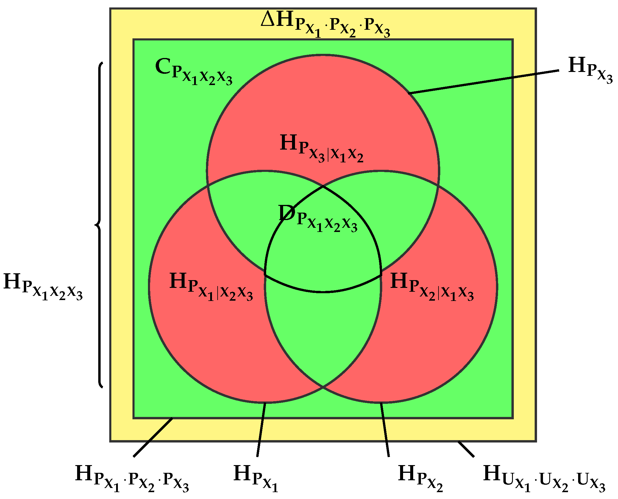
In the context of the random vector X ¯ P X ¯ , let Π X ¯ = i = 1 n P X i be the (jointly) independent distribution with similar marginals to P X ¯ and U X ¯ = i = 1 n U X i be the uniform distribution with identical support. And, consider, for example, the trivariate distribution of Figure 4 from [33].
As a matter of principle, we consider that every random variable has a residual entropy which might not be explained away by the information provided by the other variables, H P X i X i c where X i c = X ¯ { X i } . We call (multivariate) variation of information [38]—or residual information [39]—a generalization of the same quantity in the bivariate case, the sum of these quantities across the set of random variables—the red area in Figure 4:
V I P X ¯ = i = 1 n H P X i X i c .
Consider also the divergence with respect to uniformity of each X i
Δ H P X i = H U X i H P X i
with Δ H Π X ¯ = i = 1 n Δ H P X i whereby we can prove:
Δ H Π X ¯ = H U X ¯ H Π X ¯
that we interpret as the overall divergence with respect to uniformity U X ¯ of the distribution of the random vector. This is the yellow area in Figure 4.
M P X ¯ may be written in terms of the component entropies:
M P X ¯ = i = 1 n H P X i i = 1 n H P X i X i c = i = 1 n ( H P X i H P X i X i c )
and let us call M P X i = H P X i H P X i X i c , the bound information (of X i ), the amount of entropy of P X i that is bound through dependences to the marginal distributions of different orders of P X i c . Therefore, all the previously considered quantities are reducible to those about their component variables, a situation that is not too clear in Figure 4.
It proves very useful later to consider the following conditions for a given variable X i in the context of X ¯ :
  • Uniformity, P X i = U X i , whence H P X i = H U X i is maximal with Δ H P X i = 0 . The opposite of this property is determinacy whereby P X i ( x ) = δ a i ( x ) , in which case there is no uncertainty about the outcome of X i , H P X i = 0 , and Δ H P X i = H U X i   whence we may conclude:
    0 = Δ H P X i | P X i = U X i Δ H P X i H U X i = Δ H P X i | P X i = δ a i
  • Orthogonality, X i X i c , defined by P X ¯ = P X i P X i c , whence H P X ¯ = H P X i c + H P X i . In such case, since H P X ¯ = H P X i c + H P X i X i c , we conclude that H P X i X i c = H P X i and M P X i = 0 by definition.
  • Redundancy, X i X i c if the value of X i is completely determined by the value of X i c . This entails that H P X i X i c = 0 .
As a result, we see that there are bounded continua for the values of H P X i X i c and M P X i
H P X i X i c | X i X i c 0 H P X i X i c H P X i H P X i X i c | X i X i c
M P X i | X i X i c 0 M P X i H P X i M P X i | X i X i c
Theorem 1
(Multisplit source multivariate balance equations). Let P X ¯ be an arbitrary discrete distribution over the set of random variables X ¯ = { X i } i = 1 n . Then, with the definitions above,
  • The following split balance equation holds for each variable individually:
    H U X i = Δ H P X i + M P X i + H P X i X i c , 1 i n 0 Δ H P X i , M P X i , H P X i X i c H U i , 1 i n
  • The aggregate balance equation holds:
    H U X ¯ = Δ H Π X ¯ + M P X ¯ + V I P X ¯ 0 Δ H Π X ¯ , M P X ¯ , V I P X ¯ H U X ¯
We may normalize either (8) or (9) by the total sum, for instance by H U X ¯ ,
1 = Δ H Π X ¯ + M P X ¯ + V I P X ¯ 0 Δ H Π X ¯ , M P X ¯ , V I P X ¯ 1
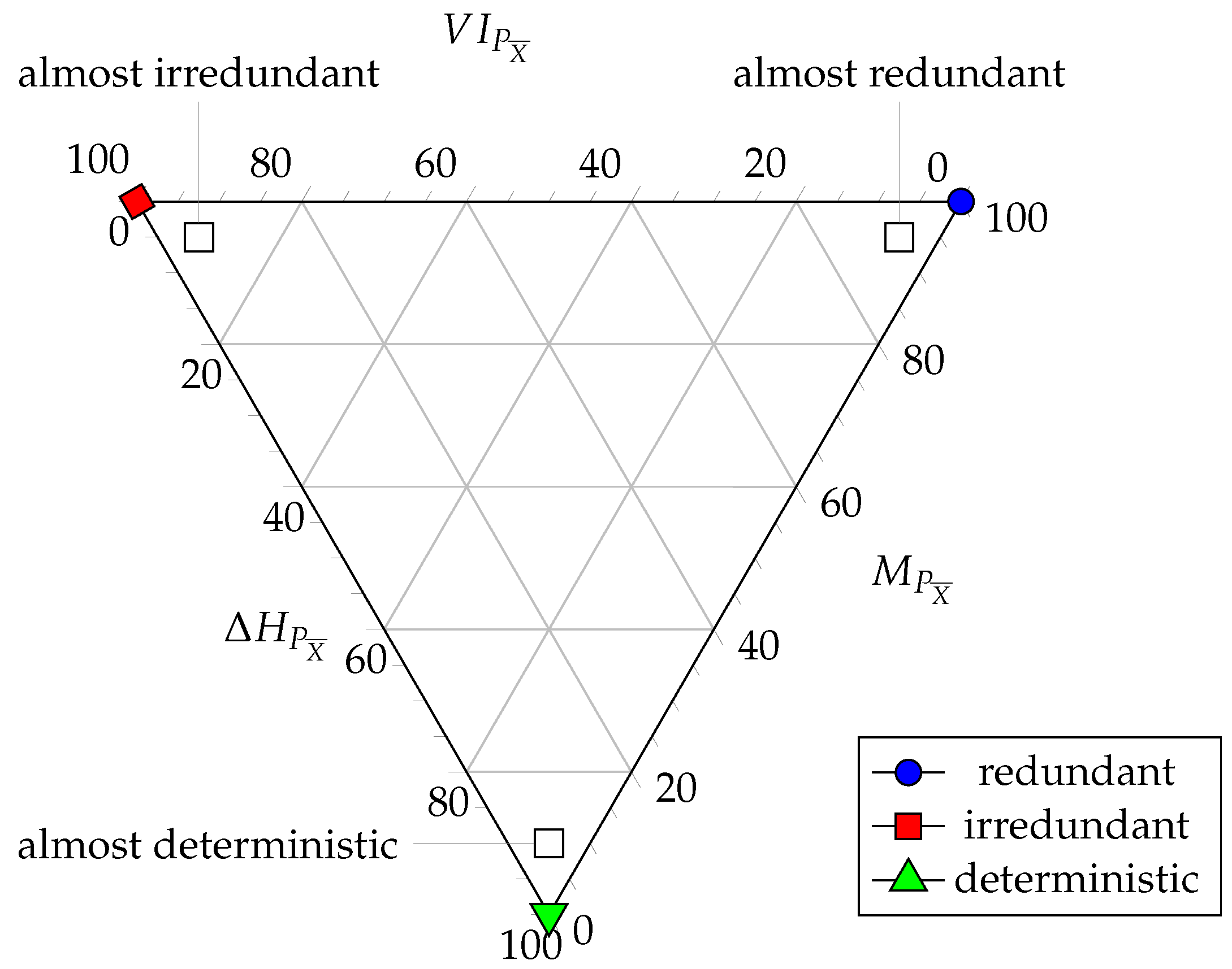
in which case the composition F ( P X ¯ ) = [ Δ H P X ¯ , M P X ¯ , V I P X ¯ ]   suggests a representation in terms of a ternary diagram that we call the aggregate Source Multivariate Entropy Triangle, (aggregate) SMET for short, with meanings:
  • If P X ¯ = Π X ¯ = Π i = 1 n P X i then F ( P X ¯ ) = [ · , 0 , · ] , is the geometric locus of distributions with independent marginals and has a high residual entropy.
  • If P X i = U X i , 1 i n then F ( P X ¯ ) = [ 0 , · , · ]   is the geometric locus of distributions with uniform marginals.
  • If P X i = P X j , i j then F ( P X ¯ ) = [ · , · , 0 ]   is the locus of distributions with identical marginals and in general high bound information.
Notice that:
  • The multivariate residual entropy V I P X ¯ is actually the sum of amounts of information singularly captured by each variable. Nowhere else can it be found and any later processing that ignores this quantity will incur in the deletion of that information, e.g., for transmission purposes.
  • Likewise, the total bound information is highly redundant in that every portion of it resides in (at least two) different variables. Once the entropy of one feature has been processed, the part of the bound information that lies in it is redundant for further processing.
  • Somewhat similar to the original interpretation, the divergence from uniformity is not available for processing. It is a potentiality—maximal randomness—of the source of information that has not been realized and therefore is not available for later processing, unlike the other entropies.
Since this latter quantity is deleterious to information transmission, a different representation to that of the usual 2-simplex suggests itself: the simplex should be rotated so that the divergence from uniformity is represented as a down-growing quantity. The rationale for this is that the lower a distribution is plotted, the less information it has at its disposal to be transmitted. Figure 5 shows a conceptual version of the SMET annotated with these intuitions.
The finer, disaggregate analysis and visualization tool is introduced by the normalization of (8). Then for each multivariate X ¯ = { X i } i = 1 n we may write for each marginal P X i the coordinates in a de Finetti diagram as F ( P X i ) = [ Δ H P X i , M P X i , H P X i X i c ]  , with similar interpretation as above, but regarding the content of a single variable. We refer to this common representation as the multisplit Source Multivariate Entropy triangle (multisplit SMET). With this new arrangement in place, the upper right-hand angle of the inverted triangle represents the locus of highly redundant variables, whereas the left-hand angle represents that of highly irredundant variables with an extensive amount of information that only pertains to them. Finally, the lower angle in the triangle represents almost deterministic variables, conveying very little information in general.
These downward-pointing SMETs solve the problem of representing the information content of a multivariate random source—using the aggregate SMET—and its individual labels—using the multisplit SMET. An R package for representing such diagrams based on the ggtern [40] package is available as [41].

2.3. A Brief Introduction to Formal Concept Analysis

In the interest of self-containment, we briefly introduce here the fundamental concepts of Formal Concept Analysis (FCA [34,42,43]). A better motivated introduction to it can be found by reading the several related chapters of [31].

2.3.1. Formal Contextualization

FCA is a procedure to render lattice theory more concrete and manipulative [34] and its use is well attested in an EDA framework both in its original and generalized extensions [44,45,46,47]. It stems from the realization that a binary relation between two sets I 2 G × M —where G and M are conventionally called the sets of formal objects and attributes, respectively—defines a Galois connection between the powersets X 2 G and Y 2 M endowed with the inclusion order [48].
The triple K = ( G , M , I ) is called a formal context and the pair of maps that build the connection are called the polars (of the context):
A 2 G , A = { m M g A , g I m } B 2 M , B = { g G m B , g I m } .
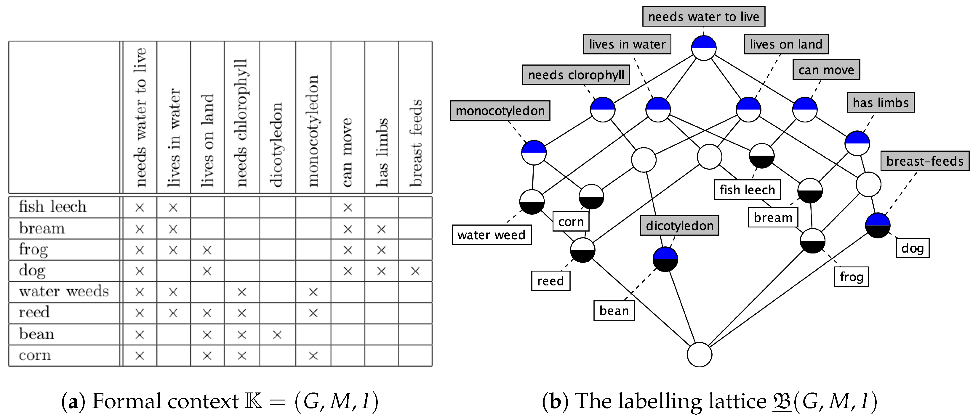
Figure 6 represents a paradigmatic example in FCA. The table in Figure 6a represents the formal context, i.e., a contextualization of the knowledge contained therein.

2.3.2. Analysing a Formal Context into Its Formal Concepts

Pairs of sets of formal objects and attributes that map to each other are called formal concepts and the set of formal concepts is denoted by
B ( G , M , I ) = { ( A , B ) 2 G × 2 M A = B A = B } .
The set of objects of a concept is called its extent while the set of attributes is called its intent, in the Fregean tradition.
The set of extents (respectively, intents) is denoted as B G ( G , M , I ) 2 G , and called the system of extents, (respectively, B M ( G , M , I ) 2 M , the system of intents.) Formal concepts are partially ordered by the inclusion (resp. reverse inclusion) of extents (resp. intents)
c 1 = ( A 1 , B 1 ) , c 2 = ( A 2 , B 2 ) B ( G , M , I ) c 1 c 2 A 1 A 2 B 1 B 2
With the concept order, the set of formal concepts B ( G , M , I ) , is actually a complete lattice called the concept lattice B ̲ ( G , M , I ) of the formal context ( G , M , I ) where meets, or infima, and joins, or suprema, are given by:
t T ( x t , y t ) = t T y t , ( t T y t ) t T ( x t , y t ) = ( t T x t ) , t T x t
For instance, the lattice in Figure 6b is the concept lattice of the formal context in Figure 6a.
By the previous definition of the order and (13) we have:
Corollary 1.
The systems of extents is isomorphic to the concept lattice, while the system of intents is (order-) dually isomorphic to the concept lattice, therefore the systems of extents and intents are, themselves, (order-) dually isomorphic.
The sets of formal objects and attributes can be embedded into these lattices by means of the concept-inducing mappings:
γ ¯ I : G B ̲ ( G , M , I ) μ ¯ I : M B ̲ ( G , M , I ) g γ ¯ I ( g ) = ( { g } , { g } ) m μ ¯ I ( g ) = ( { m } , { m } )
obtaining the sets of object- and attribute-concepts  γ ¯ I ( G ) B ( G , M , I ) , μ ¯ I ( M ) B ( G , M , I ) .
For instance, for object corn and attribute breast-feeds we have:
γ ¯ I ( corn ) = ( { corn } , { needs water , lives on land , needs clorophyll , monocotyledon } ) μ ¯ I ( breast feeds ) = ( { dog } , { breast - feeds } )
Note that these characterizations are contextualised with respect to the particular context of Figure 6a, that is, with more breast-feeding mammals in the set G, the concept for  μ ¯ I ( breast feeds ) would have those extra objects.

2.3.3. Interpreting Concept Lattices

Most concept lattice-building algorithms available output order (Hasse) diagrams developed to easily describe partial orders. Concept lattices can profitably be represented and grasped in such form: nodes in the diagram represent concepts, and the links between them the hierarchical partial order between immediate neighbours. A more gentle introduction to this is ([31], Chapter 3.)
For the purpose of reading extents and intents off the order diagram, concepts could be annotated graphically with a complete labelling, by listing for each concept the set of object labels in the concept extent and the set of attribute labels in the concept intent. But since this implies repeating many times each object and attribute throughout the lattice the following, reduced labelling is preferred, as in Figure 6: we put the label of each attribute only in the highest (most abstract) concept it appears, and the label of each object only in the lowest (most specific) concept it appears.
This is performed using the concept inducing mappings: we write each object just below the corresponding object–concept and each attribute just above its attribute-concept. This is the type of labelling shown throughout the paper—for instance, in Figure 6b for γ ¯ I ( corn ) and μ ¯ I ( breast feeds ) —and the most usual, though different lattice-building tools use variations of it.

2.3.4. Synthesising a Context for a Complete Lattice

In fact, the concept-forming maps allows us to discover the relation I within B ̲ ( G , M , I ) . For that purpose, recall that a subset Q of an ordered set L , is called join-dense is every element of L is the join of a subset of Q, and order-dually for being meet-dense.
Proposition 1.
Let ( G , M , I ) be a formal context and B ̲ ( G , M , I ) be its concept lattice. Then: γ ¯ I ( G ) is join-dense in B ̲ ( G , M , I ) , μ ¯ I ( M ) meet-dense in B ̲ ( G , M , I ) and for g G , m M ,
g I m γ ¯ I ( g ) μ ¯ I ( m ) .
Proof. 
See, e.g., ref. [31], 3.7 and 3.8.    □
By analogy with this procedure, we may state no less than a universal representation theorem for complete lattices in terms of FCA:
Theorem 2
(Synthesis Theorem of FCA). Let L , be a complete (order-)lattice and assume there exists two mappings γ ¯ : G L and μ ¯ : M L such that γ ¯ ( G ) is join-dense in L and μ ¯ ( M ) is meet-dense in l. Define I G × M by g I m γ ¯ ( g ) μ ¯ ( m ) , then L and B ̲ ( G , M , I ) are isomorphic, L B ̲ ( G , M , I ) . In particular L B ̲ ( L , L , ) .
Proof. 
See, e.g., ref. [31], 3.9.    □
For practical purposes, this means that the information in the formal context of Figure 6a can be filled from the relative positions of object- and attribute-concepts in the lattice of Figure 6b.
The quotient sets of the sets of formal objects and attributes through the concept-inducing mappings are important to reduce the workload: given ( G , M , I ) , we may define its reduced context as K o = ( G / γ ¯ I , M / μ ¯ I , I o ) where, using standard notation for quotient relations,
( [ g ] ker γ ¯ I , [ m ] ker μ ¯ I ) I o g I m .
Proposition 2.
If ( G , M , I ) is a formal context, then its concept lattice and that of its reduced context are isomorphic:
B ̲ ( G , M , I ) B ̲ ( G / γ ¯ I , M / μ ¯ I , I o ) .
Proof. 
This is an easy corollary of Theorem 2.    □
Due to the corollary we can, essentially, work with a single representative per block. However, rather that being in this extremely reduced form, typically contexts are clarified when they are both row-clarified—no two rows are identical—and column clarified—no two columns are identical.
For finite contexts, the type that appears mostly in data analysis, the reduction actually has to be understood in terms of the join- and meet-irreducibles of complete lattices. Recall from order theory that a subset Q is join-dense in a complete lattice L = L , if it includes all the join-irreducibles of the lattice L , J ( L ) Q , those elements that cannot be obtained by joins of other elements. Likewise, a meet-dense subset must include the meet-irreducibles M ( L ) Q . Then a simple corollary of the synthesis theorem is:
Corollary 2.
Let L = L , be a complete finite lattice. Then L B ̲ ( J ( L ) , M ( L ) , ) .

3. Results

This paper contributes to the metaphor of Supervised Classification Tasks are Information Channels of Section 2.1 by expanding its use for the modelling and EDA of MLC tasks. For that purpose we bring to bear two types of tools:
  • lattice theory in the form of Formal Concept Analysis (FCA [34,42]), as described in Section 2.3, to extract the qualitative information in MLC data.
  • Compositional Data Analysis (CoDa [49,50]) specifically as it applies to the entropic compositions of joint distributions [33,35] described in Section 2.2, to measure the quantitative information in MLC data.
Note that we leave the formalization of classifier evaluation for future work.

3.1. An Analysis of Information Content of MLC Task Data

The crucial affordance of the enriched metaphor is to realise that the labels are logically prior to the observation features and that we can use the technique of FCA to analyse labelsets. Specifically, recall that FCA is an unsupervised data mining technique.
Definition 1
(Formal Contexts of a MLC task). Let L be a set of labels, and D = { ( y j , x j ) } j = 1 n be a MLC dataset as described in the introduction. Then:
  • The formal context D L = ( G , L , I ) is the labelling context (of samples) of D , built using the set of labels L as formal attributes, with | L | = l , each sample index as a formal object i G , with | G | = n , and each bitvector-encoded sample labelset { y i } i = 1 n , y i 2 l as the i-indexed row of the incidence matrix I i · = y i .
  • The formal context D F = ( G , F , R ) is the observation context (of samples) of D built with F a set of features, | F | = m , the same set of formal objects G and each observation vector { x i } i = 1 n is the i-indexed row of the incidence R i · = x i .
We call their corresponding concept lattices,
  • The labelling lattice B ̲ ( G , L , I ) , short for “the concept lattice of the labelling context”;
  • The observation lattice B ̲ ( G , F , R ) , analogously.
Figure 7 represents a part of the labelling context D L of the emotions dataset and its labelling lattice.
Note that while the labelling context is boolean and the labelling lattice is supported by standard FCA, the observation context is real-valued, or at least multi-valued, and is only lattice-forming under stringent algebraic conditions [51,52,53]. For that reason the analysis of the information content of the observations and transformed observations will be left for future work. However the following lemma is self-evident—recall that the context apposition is the row-by-row concatenation of formal contexts:
Lemma 1.
Let D = { ( y j , x j ) } j = 1 n be a MLC dataset. Then, the apposition of the labelling and observation contexts D = D L D F contains all and nothing but the data in the dataset.
In the following we develop the trope that although the data are the same, the information gleaned/issuing from the formal context is much richer. In this paper, we concentrate on the labelling context.

3.1.1. Information Content of MLC Sources: A First Theoretical Analysis

Clearly with the previous modelling, the labelling context captures the information in the stochastic source Y ¯ , and providing the affordances of FCA as an EDA technique [45,54]:
Hypothesis 1.
Relevant notions in an MLC dataset labelling correspond to relevant notions in the FCA of the labelling context D L and vice versa.
For instance, the following are affordances of using formal contexts to analyse the MLC source:
  • Labelsets are object intents of D L and they can be found through the polar of observations. As a consequence we have:
    Corollary 3.
    The labels in L are hierarchically ordered in exactly the order of the systems of intents prescribed by B ̲ ( G , L , I ) , that is, the dual order, and the object concepts of observations γ ¯ I ( G ) are a set of join-dense elements of the lattice, and they generate the lattice of intents by means of intent (labelset) intersection.
    Proof. 
    Recall that for an observation i G its labelset is y i = { i } I which is precisely its intent, so the intents of γ I ( G ) are the labelsets in the task. By the synthesis Theorem 2 γ ¯ I ( G ) are a set of join-dense elements of B ̲ ( G , L , I ) and after Equation (13) their intents generate B ̲ L ( G , L , I ) , the system of intents, by intersection.    □
  • FCA is capable of providing previously unknown information on the set of labels through the concept lattice construction.
    As an example, recall that the set of intents of the labelling context is B ̲ L ( G , L , I ) 2 L . Then we have:
    Proposition 3.
    The LP transformation and its derivatives only need to provide classifiers for the intents of the join-irreducibles of B ̲ ( G , L , I ) .
    Proof. 
    We know that only labelsets are used by the LP transformation and its derivatives so the general setup for this task is addressed by Corollary 3. But, due to Proposition 2, to reconstruct the information we only need one of the representatives of each block of the partition. Finally, due to Corollary 2 we only need the labelsets of the join-irreducible blocks in order to reconstruct B ̲ ( G , L , I ) .    □
    Several remarks are in order here. First, depending on the dataset, this may or may not be a good reduction in the modelling effort. Also, note that the information about occurrence counts is lost, therefore:
    Guideline 1.
    Naive information fusion strategies would only work in the 100% accuracy case—e.g., for a given observation use the classifiers for the intents of the meet-irreducibles to obtain individual characterizations and then intersect them.

3.1.2. Qualitative Information Content of MLC Sources: An Exploration

Since the first result of this re-framing of the MLC task in terms of FCA is a broadened view of issues, in order to further investigate the labelling contexts or multilabel sources, we analyse three types of standard scales, that is, prototypical formal contexts [34] (Section 1.3Section 4), each of which shows in its concept lattice some type of ordering relationship between the attributes.
We use the reduced labelling to annotate lattices, that is, for each formal concept:
  • The set of labels it represents is the union of all labels in the order filter of the concept, that is, looking upwards in the lattice.
  • The set of instances covered is the union of all instances in the order ideal of the concept, that is, looking downwards in the lattice.
Figure 8 shows these types of contexts and the relationship they generate among its labels in the form of concept lattices for order n = 3 .
  • Nominal scales of varying order—e.g., in Figure 8a,d. Note that the nodes in the concept lattice annotated with the labels is an antichain, that is a set with no ordering between its elements [31], whence we take them to express (mutual) incompatibility between labels.
  • Contra-nominal scales of varying order—e.g., in Figure 8b,e for order 3. Like the previous case nodes in the concept lattice annotated with the labels is also an antichain. They are traditionally associated with incompatibility and partition [34].
  • Ordinal scales of varying order—e.g., in Figure 8c,f. The set of formal concepts annotated with the labels is a total chain, a set with a total ordering between its elements [31], traditionally related to rank order.
True to the hypothesis stated above, we can develop intuitions with respect to MLC tasks whose labelling context belonged in some of these tasks:
  • We would expect BR-like transformations to be good for a nominal labelling context.
  • We would expect CC-based strategies to be good for ordinal labelling contexts, provided the implication order between labels, as manifested in the concept lattice, was known at training time and, somehow, profited from.
  • It is difficult to know what strategy could be good for a contra-nominal labelling context. As a first intuition, considering that it is the contrary context to the nominal scale of the same order, we would expect BR to be also effective.
Note that the important formal concepts are those with blue upper halves, in the case of the standard scales of Figure 8, the meet-irreducibles of the labelling context. We further posit that:
Hypothesis 2.
The suborder of the meet irreducibles of labelling lattice B ̲ ( G , L , I ) may help predict the performance of the different problem transformation strategies in MLC for a particular dataset.
We will try to experimentally support our hypotheses next.

3.1.3. Quantitative Information Content of Boolean Contexts: A Theoretical Analysis

Statistical processing of labelling contexts as multivariate sources is based upon the following proposition, where labelling contexts ( G , L , I ) behave as if they were multivariate distributions of their labels—acting as random variables—and their instances—acting as (empirical) occurrences.
Proposition 4.
Labelling contexts ( G , L , I ) are the result of sampling random stochastic sources of labelsets by means of observations.
Proof. 
Retaking the quantitative reasoning from the previous section, recall that the concept-forming function γ ¯ I induces a partition ker γ ¯ I on G by equality of labelsets: ( i 1 , i 2 ) ker γ ¯ I { i 1 } I = { i 2 } I . By an abuse of notation, denote the subset of labelsets obtained by the polar of intents acting on the observations by G B L ( G , L , I ) . Define a measure on the labelsets of the observations concepts as n ( y ) = | [ y ] ker γ ¯ I | , that is, n ( y ) is the occurrence count of the labelset y , in the data so that
n = y G n ( y ) .
Then we may estimate the probability of each labelset, taken as a boolean vector, as:
P Y ¯ ( y ) n ( y ) / n i G , y = { i } 0 otherwise .
Note that the actual form of the probability estimator—relative frequency as in the example or another, smoothed, estimator, etc.—does not invalidate the conclusion.    □
By means of Proposition 4, we can reason about the sampling of the stochastic variables Y ¯ and X ¯ —the dataset—in terms of the contexts above, and vice versa.
  • For instance, we expect the sampling to be good enough l n so it is safe to suppose that no two identical labels are predicated of the same set of objects.
    Guideline 2.
    MLC datasets should be label-clarified, that is, no two labels should describe the instances in the same way.
    Notably, this holds on standard testing datasets (e.g., those in [8] and Table 1), so Therefore we expect the partition on labels induced by μ ¯ I to be ker μ ¯ I = ι L where ι L is the identity on L.
  • Regarding the equivalence in γ ¯ I , in [55] we introduced a general framework to interpret the structure of the set of labels in terms of FCA and used it to improve a standard resampling technique in ML: n-fold validation. The rationale of this technique and an experiment demonstrating it can be found in Section 3.2.
  • Finally, the existence of ker γ ¯ I and the probability measure introduced in (15) on its blocks warrants the validity of the source multivariate entropy decompositions of labelling contexts and their Source Multivariate Entropy Triangles (SMET) of Section 2.2.
Corollary 4.
The quantitative information content of a labelling context can be accurately represented using SMETs.
Proof. 
Specifically, (8) on the distribution of (15) allows us to observe the information balance on the individual labels, while (9) on the same distribution allows us to observe the aggregate information of the dataset.    □
Leveraging the previous results we may study sources of labelsets with the SMET.
Hypothesis 3.
Instantiating the procedure of building SMETS in Section 2.2 on standard scales we expect nominal and contra-nominal scales to have the same quantitative information—since they are contrary scales while it has to be very different for ordinal scales, given the symmetry properties of entropies.
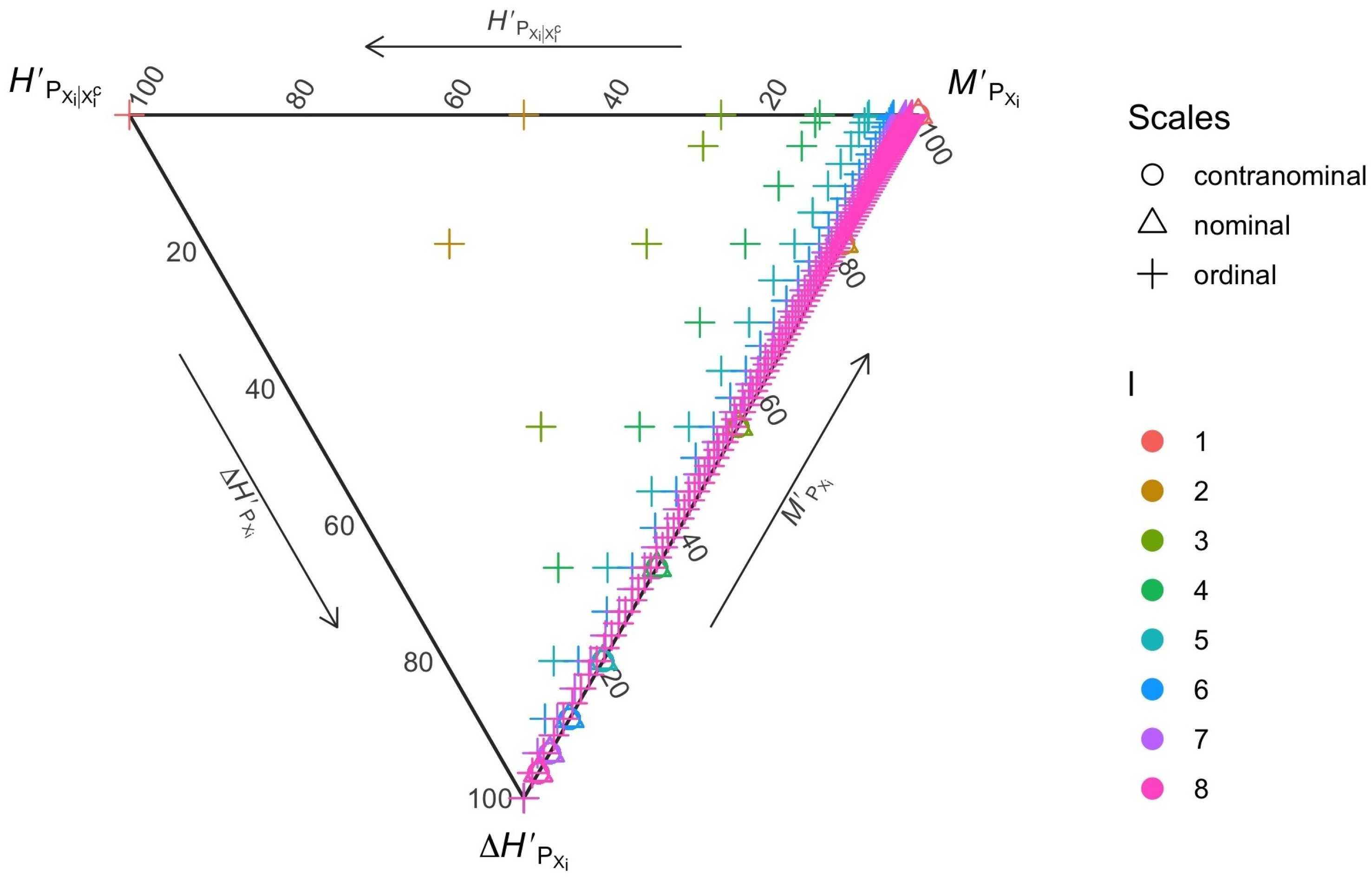
To test this hypothesis, Figure 9 shows the aggregate information content of several nominal, contra-nominal, and ordinal scales of different order, where this order equals the number of labels of the scale.
The examples show:
  • As expected, nominal and contra-nominal scales have the same, totally redundant, average information content—since they lie on the H P X i | X i c = 0 line in Figure 9—and both show a tendency to a decreasing average information content as the order of the scale increases, from an initial high average information content, but still redundant.
  • However, ordinal scales start from an intermediate level of irredundant information and 50 % randomness and slowly mount towards higher but more correlated average information contents. By the time the order reaches 2 8 = 256 the information is totally redundant with high degree of randomness.
Regardless, the previous behaviour is only on average and we should wonder what the individual content of the labels in each case actually is. Figure 10 shows the information content of all labels for standard scales of ordinal, nominal and contra-nominal type for orders 2 l , l { 2 , 3 , 4 , 5 , 6 , 7 , 8 } .
Note that:
  • For nominal and contra-nominal scales, all the labels have exactly the average information content. This is immediate for nominal labels, and would be expected to follow by the relation between nominal and contra-nominal scales and the symmetry properties of entropy. Note that one singular label can, in principle, be perfectly predicted from the rest since each is completely redundant, that is, they lie in the line H P X i | X i c = 0 . Note also that labels belonging to high order scales have very little information content: that is, they resemble detection phenomena—one majority vs. one minority class.
  • For ordinal scales, for the same order, there is a rough line for the label information parallel to the left-hand side of the triangle, ending in the bottom vertex. The information is the more correlated the higher the order 2 l . Note that some pairs of labels have the same information content—e.g., those with complementary distributions of 0 and 1. Clearly, the higher the proportions of 1 (respectively 0) the less information a label bears, and this reaches the bottom apex since the last label is a deterministic signal (always on).

3.2. FCA-Induced Stratified Sampling

For reasons of completion, we include here some results which support our main Hypothesis 1. They have previously been introduced to a reduced audience in [55].
Consider the MLC induction and assessment procedures in step 4 of the pseudo-algorithm in Section 3.4: To generate train and test divisions of the original data we may split the original context D into two subposed subcontexts of training D T and testing D E data so that D = D T / D E  [55,56]. Note that:
  • Since the samples are supposed to be independent and identically distributed, the order of these contexts in the subposition, as indeed the reordering of the rows in the incidence, is irrelevant.
  • The resampling of the labelset context D L is tied to the resampling of the observation context D F : we decide on the labelset information and this carries over to the observations.
Since the data are a formal context, FCA suggests that an important part of the information contained in it comes from the concept lattice, hence we state the following:
Hypothesis 4.
FCA allows us to spot possible problems with the classifier induction and validation schemes using resampling.
  • (Qualitative intuition) A necessary condition for the resampling of the data D into training part D T and testing part D E to be meaningful for the MLC task, is that the concept lattice of all of the induced labelling subcontexts D L T and D L E be isomorphic:
    B ̲ ( D L ) B ̲ ( D L T ) B ̲ ( D L E )
  • (Quantitative intuition) The frequencies of occurrence of the different labelsets in the blocks of ker γ ¯ I are also important.
The rationale for this hypothesis is straightforward. Due to the identification of object intents and labelsets, we know that to respect the complexity of the labelset samples in each subcontext, one sufficient condition is that one of the labelsets associated with each block in the partition ker γ ¯ I is accorded to each of the subcontexts.
If this is the case, then the sampled subcontexts being join- and meet-dense, will generate isomorphic concept lattices. Since they each are a clarification of the original context D L , their concept lattices are all isomorphic.
However, if we only retained the meet- and join-irreducibles to obtain these concept lattices, then the labelsets of reducible attributes would be lost and this would change the relative importance of the samples (both labels and observations, remember), which will therefore impact the induction scheme of the classifiers. Hence not only the labelsets but also their frequencies of occurrence are important.
The above hypothesis suggests the following guideline:
Guideline 3
(Stratified resampling of MLC tasks). Resampling of MLC data should be carried out modulo ker γ ¯ I so that the concept lattices of the training and testing folds are isomorphic to that of the original context.
Note that this amounts to standard stratified sampling on single-label classification tasks.
Following this guideline, however, comes at a price, when there are hapaxes—under-represented cases—in the data. If we choose, for instance, to maintain 80 % of the data for training and 20 % for testing, regardless of these proportions, stratified sampling will force us to include all hapaxes with the following deleterious consequences:
  • The relative frequency of the hapaxes will be distorted (overrepresented) with respect to other labelsets.
  • We will be using some data (the hapaxes) both for training and testing, which is known to obtain too optimistic performance results in whichever measure.
Furthermore, if we use, e.g., k-fold validation we have to repeat this procedure and ensure that the resampling is somehow different. A usual procedure is to distribute the original dataset into k blocks in order to aggregate k 1 of them into the training dataset  D T and use the leftover as the testing dataset D E . This can only compound the previous problem, therefore the following guideline suggests itself:
Guideline 4
(Dealing with hapaxes). When using k-fold validation and stratified resampling on MLC tasks we should have a procedure to deal with hapaxes of up to k 1 counts.
In the following sections we will suggest one such procedure, namely thresholding and reassignment of labelsets to the closest one in some distance. Note that other practitioners do not deal with this problem [17].

3.3. Experimental Validation

To try and test our hypotheses, guidelines, and tools, we carried a number of EDA tasks on MLC data.

3.3.1. Exploring a Clustering Proposal on MLC Datasets

Recall that Table 1 shows a summary table of measures of many MLC datasets. The authors of [25] proposed a clustering hypothesis for some of those datasets obtained through a miscellanea of criteria. Roughly, it consists of eight clusters of differing sizes and affinities, and is, to our knowledge, the only clustering proposal based on objective criteria for MLC datasets. Interestingly, neither the entropic decomposition visible in the SMETs or any measures related to the concept lattice of the labelling context were used in this clustering.
Figure 11 shows the results of showing that clustering in the SMET by plotting the aggregate measure across labels.
We can see that this clustering hypothesis of [25] is clearly not sustained by the entropic analysis, as the aggregate SMET shows:
  • Limited clustering: except for cluster D7—and perhaps D3—the rest of the clusters show great entropic dispersion.
  • Overlapping: sometimes, exemplars of one cluster lie beside an immediate neighbour or another—e.g., instances of D1 and D2.
  • Extreme dispersion: it does not seem to be justified calling D5—or perhaps even D8–a cluster from the entropic point of view.
Note that no dataset is visible for cluster D6, since none of the datasets in the cluster was available in the mldr repository where the data were accessed.

3.3.2. Exploring the Clustering Hypothesis at the Dataset Level

To probe further, Table 2 shows a selection of low- to middle-complexity datasets from the clustering described in [25].
The multisplit SMETS for the selected datasets are shown in Figure 12.
Recall from Section 2.2 that the multisplit SMET conveys not only how deterministic the individual labels are, but also how redundant with respect to the rest of the set of labels.
Despite the fact that each of these datasets belongs to a different cluster we can already see some common traits:
  • eurelexev is an extreme case of a dataset with many redundant features most of which are heavily imbalanced. This is a dataset of multilabel detection, not classification. Furthermore, its average and the coordinates of the individual labels suggest that it resembles either a nominal or a contra-nominal scale, that is, labels appear in any possible combination (contra-nominal scale) or mutually exclusively (nominal scale, cfr. Figure 9).
  • To a certain extent, this is also the classification for rcv1sub1, although the slight separation of many values may suggest that there are substructures in the form of ordinal scales.
  • birds, enron and slashdot are eminently label detection tasks with a minority of labels—the ones with higher bound information—which might be subject to classification. The distinction between them is in the amount of bound information overall: the more bound information the farther to the right the cloud of points is.
  • Specifically, the birds task clearly has mostly detection labels. Not only is the empty labelset the majority class, but also, there are many hapaxes for the individual labels. Some labelsets may be distilled for poorly balance detection tasks disguising as binary classification tasks.
  • flags and emotions [57] seem to be purely MLC tasks with fairly uniform label distributions and some degree of bound information between them. As per the previous discussion on the whole set of labels, they might even be considered in the same cluster.

3.3.3. Stratified Sampling in MLC Tasks

The following analysis is carried out on the emotions dataset [57], as pre-processed and presented by the mldr R package [26]. It was also presented to a reduced audience in [55] and reproduced here to strengthen our case.
Basic EDA of the labels. Since we are only considering the set of labels Y ¯ , we extracted the histogram of the labelsets { y j , n ( y j ) } j J from the dataset and considered a set of minimal frequencies of occurrence n T { 0 , 1 , 4 , 9 , 16 , 25 } acting as thresholds based on it. The case n T = 0 actually represents the original dataset in Figure 12b, and shows the information balance of each of the six labels of emotions as well as the average balance for them all.
We see that most labels are rather random, with ‘relaxing-calm’ completely so. No label is completely specified by the rest of them, nor is any totally independent. This in essence means that the dataset is truly multilabel.
Disposing of hapaxes to improve stratified sampling. Previous analyses of the histogram of labelsets made us realize that this dataset is not adequate for resampling due to hapaxes and in general low-counts of many labelsets [56]. This applies to most MLC datasets used at present [8].
Guideline 5.
To dispose of hapaxes without disposing of samples we must re-assign each to a more frequent labelset.
The rationale for this decision is because we consider hapaxes errors in label codification, and assume that the “real” labelset is the closest non-hapax in Hamming distance—recall that the Hamming distance between two sequences of bits of identical length is the number of positions in which they differ. However, this re-assignment changes the histogram of labelsets resulting in a decrease in the information independence of the labels and the dataset in general.
To explore this trade-off, at each threshold n T , a labelset y was considered a generalized hapax if n y < n T . For each threshold n T we calculated the Hamming distance between each generalized hapax y n T and the non-hapaxes, and found the set of those closest to it. Then we re-assigned y n T to one of them uniformly at random (allowing for repetitions). Note that an alternative strategy would have been a scheme considering the original frequencies in the histogram, to simulate a rich-get-richer phenomenon. But such a procedure would decrease the source entropy more than the one we have chosen.
This reassignment defined a new dataset whose information balance was represented by the multisplit SMET whence Figure 13 ensued.
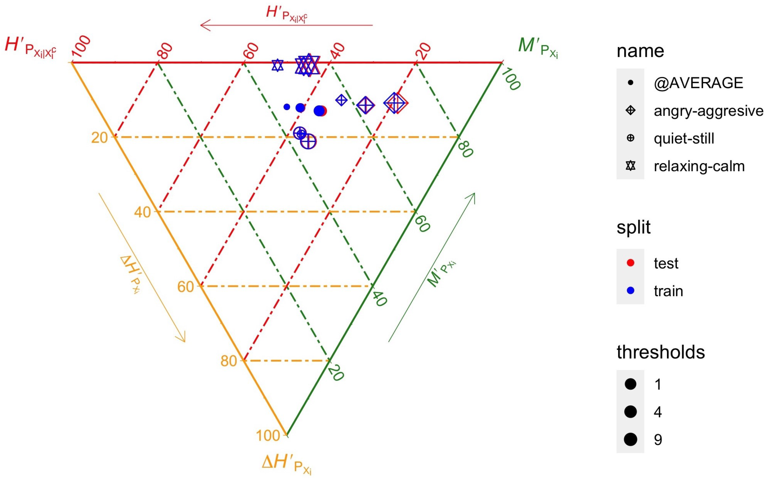
What we can see is a general tendency to the increment of the total correlation as the thresholds increase manifested in a right-shift. But this entails that the individual distinctiveness of each label is diminished. See, for instance, the case for ‘angry-aggressive’ that can actually be predicted from the other labels when n = 25 , confirming that too aggressive a threshold will substantively change the relative information content of the labels in the dataset.
Choosing the adequate threshold. Note that a threshold of n is needed to request an ( n + 1 ) -fold cross-validation of any magnitude about the dataset, since all labelset will have at least ( n + 1 ) representatives for the stratified sampling requested by the cross validation procedure. Next we explore whether it is possible to balance the identical sampling property on train and test, yet avoid too much loss of information content.
Figure 14 depicts a choice of thresholds typically used in validation—1, 4 and 9, corresponding to 2-, 5-, and 10-fold validation—for three differently behaving labels—‘angry-aggressive’, ‘quiet-still’, and ‘relaxing-calm’—and the average of the dataset, both for the ensembles of training and testing folds.
  • As applied to the estimation of the entropies, the ( n + 1 ) -fold validation yields the same result in train and test, the sought-for result.
  • We can see the general drift towards increased correlation in all labels, but much more in, say, ‘angry-aggressive’ than in ‘quiet-still’.
  • For this particular dataset, a threshold of n T = 4 with 5-fold validation seems to be a good compromise for attaining statistical validity vs. dataset fidelity.
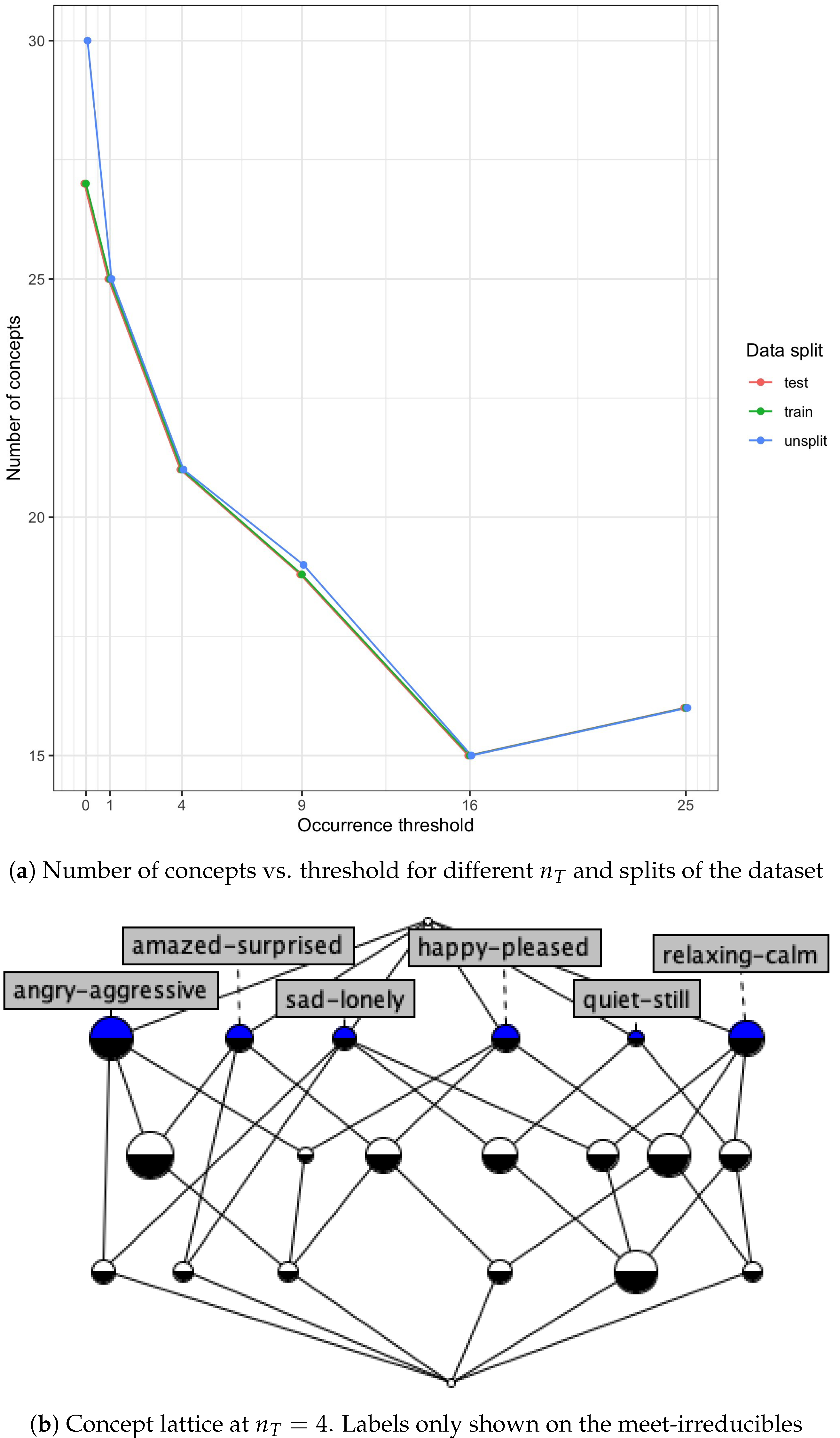
FCA confirmation. To strengthen the validity of the last two conclusions, we calculated the number of concepts of all of the train and test label contexts using the fcaR package [59]. After creating the contexts, we clarified and obtained the lists of concepts, then we compared the cardinality of the training and test concept lattices both for the unsplit dataset—after reassigning the generalized hapaxes, when needed—and the ( n + 1 ) -cross validated versions. The results are shown in Figure 15a.
As expected, for n T = 0 the difference in number of concepts between the non-sampled and sampled versions of the dataset make it non-adequate for appropriate sampling. Note that it is a fluke of the dataset that both the training and test subcontexts have the same number of concepts as some of the hapaxes are singletons.
The training and test splits had the same number of concepts for every other threshold. For n T { 1 , 4 , 16 } , the number of concepts was constant among folds, but due to the randomness inherent in sampling for n T { 9 , 25 } one of the folds was different.

3.4. Extending the Classification is Information Transmission Metaphor to MLC Tasks

With the affordances of the previous analyses from Section 3.1Section 3.3 we can undertake the improvement of the methodology for carrying out MLC tasks that is our research goal. First we instantiate the original metaphor for MLC tasks:
Metaphor 3
(Supervised MLC Tasks are Information Channels). MLC is an information channel—depicted in Figure 16—where:
  • Y ¯ is a Source of information in the form of a partially accessible random vector of binary variables.
  • X ¯ is the encoding of that information in the form of vectors of observations, x X ¯ .
  • The transformed Z ¯ are the result of conformed, noisy transmission of observation vectors.
  • The classified Y ^ is a random rector, the result of decoding the received information through the classifier, considered as a Presentation of information for downstream use.
Figure 16. Basic scheme for multilabel classification: Y ¯ and Y ^ are the source and presentation random vectors, X ¯ the observation and Z ¯ the transformed observation random vectors.
Mathematics 12 00346 g016
And finally we use those results to flesh out the pseudo-algorithm Figure 2 previously presented. The final result is shown in Figure 17.

3.5. Discussion

The use of FCA for explicitly modelling the MLC task was first invoked, to the best of our knowledge, in [55,56]. This work, however, presents the first instance of merging both qualitative representations—FCA–and quantitative measures—the different SMETs—as a model of the information sources in a particular kind of ML task, the MLC case.
In this respect, in Section 3.1.2 “information content” has to be understood as quality of information, whereas in Section 3.1.3 as quantity of information. But both are valid readings of the information content of the labelling context: our approach renders feasible the study of both facets of information, unlike each technique on its own. Specifically, we go beyond the intent of Shannon in characterizing sources of data [32] in that we provide the model for a type of qualitative information, the concept lattices of the labelling subcontexts. In this respect this paper tries to go beyond the paradigm of (quantitative) Information Theory.
Specifically, in Section 3.1.1 we explored the standard scales as candidates to interpret stereotypical qualitative behaviours of the set of labels. Later, in Section hand in hand with quantifying techniques for the information content of MLC datasets, the aggregate and multisplit SMETs. We concluded that three of the main types of standard scales of FCA, nominal, contra-nominal and ordinal carry very different quantities of informations both aggregated and on a per-label basis.
Further, using the quantitative exploratory techniques we analysed a sample of tasks of the clustering in [25] and found evidence to challenge it: possibly, only 3 clusters are visible:
  • A purely MLC dataset cluster with flags and emotions, with stochastic labels of high irredundancy.
  • A cluster of datasets of mixed detection- and classification-oriented features with varying degrees of redundancy, as in birds, enron and slashdot, and
  • A cluster of datasets of (almost purely) detection tasks with detection-oriented features, viz. eurelexcd and rc1sub1.
This tries also to push the envelope in providing a new model for statistical sources of data that sustain several hypotheses to further understand, support and guide statistical and ML-related techniques, like clustering or n-fold validation, in the context of the MLC task. Once and again the generality of the approach to qualitative description of data provided by FCA and to quantitative measurement of information provided by the entropy balance equations and entropy triangles allows us to state that this will be a fruitful partnership to explore other ML tasks.
For instance, notice how the analysis carried out in the previous section acts as a guide for further evaluation of MLC: recall that the original task is to evaluate the techniques for transforming the MLC problem into standard classification problems. In further work, these results will be used to pair up certain transformation strategies with certain types of datasets so as to provide practitioners with clear guidelines as to how to proceed on new, unseen MLC datasets. Immediate suggestions to do so are the development of factorization algorithms for lattices of labelsets, so that the MLC problem is itself factorized in as many subproblems. Proposition 3 is already a step in this direction.
All interactive R notebooks and code embodying the analyses described in this paper are available from the authors upon request.

4. Conclusions

In conclusion, we have proven that the formalisation of the MLC task can profit from using more formal backgrounds than the framework of predictive inference. In particular, this is undistinguishable from understanding the ML training and operating pipeline as an information communication channel, as proposed by Shannon in the last century and illustrated in Figure 18.
Fleshing out this metaphor stand the contributions of this paper:
  • A refinement of a meta-model for MLC tasks: the information channel model that includes joint but distinct characterizations of qualitative and quantitative aspects of information sources (see Figure 18) including:
    -
    An methodology for modelling and exploration of MLC labelling contexts D L = ( G , L , I ) based on FCA.
    -
    Novel measures and exploratory techniques for MLC dataset characterization from first principles based on information theory—the aggregated and multisplit SMETs—which are representations of the balance equation in three variables F ( P Y ¯ ) = [ Δ H P Y ¯ , M P Y ¯ , V I P Y ¯ ] .
  • This joint quantitative and qualitative model has allowed us to state:
    -
    Several Propositions and Corollaries about the characterization of MLC tasks with FCA- and entropic decomposition-related tools.
    -
    Several Hypotheses on the inner workings of MLC tasks—e.g., Hypotheses 1–4.
    -
    Several Guidelines for the development of “good” datasets for MLC—e.g., as in Guidelines 1–5.
  • A challenging of previous results on clustering MLC datasets on the grounds of the data analysis carried out with the newly introduced qualitative and quantitative techniques.
All in all, our results suggest that better and more complex mathematical formalization of datasets and tasks in ML can bring about a better understanding of them. Whether this can be used to pave the way for better classifiers in MLC is a question for further work. For this next enterprise, we have already obtained hypotheses and tools to match those that are applied here to MLC sources so that in the future their integration runs more smoothly.

Author Contributions

Conceptualization, F.J.V.-A. and C.P.-M.; methodology, F.J.V.-A. and C.P.-M.; software, F.J.V.-A.; validation, C.P.-M.; formal analysis, F.J.V.-A. and C.P.-M.; investigation, F.J.V.-A. and C.P.-M.; resources, F.J.V.-A. and C.P.-M.; writing—original draft preparation, F.J.V.-A.; writing—review and editing, C.P.-M. and F.J.V.-A.; visualization, F.J.V.-A.; supervision, F.J.V.-A. and C.P.-M.; project administration, F.J.V.-A. and C.P.-M.; funding acquisition, F.J.V.-A. and C.P.-M. All authors have read and agreed to the published version of the manuscript.

Funding

This research was funded by the Spanish Ministerio de Ciencia e Innovación grant number PID2021-125780NB-I00, EMERGE and Línea de Actuación No 3. Programa de Excelencia para Francisco José Valverde Albacete. Convenio Plurianual entre Comunidad de Madrid y la Universidad Rey Juan Carlos.

Data Availability Statement

Data are contained within the article.

Conflicts of Interest

The authors declare no conflicts of interest.

Abbreviations

The following abbreviations are used in this manuscript:
BRBinary Relevance
CCClassifier Chains
CDAConfirmatory Data Analysis
CMETChannel Multivariate Entropy Triangle
CoDaCompositional Data (Analysis)
EDAExploratory Data Analysis
LPLabel Powerset
MIMutual Information
MLCMultilabel Classification
PPresentation (in Figures)
PCCProbabilistic Classifier Chains
SSource (in Figures)
SMETSource Multivariate Entropy Triangle

References

  1. Boutell, M.R.; Luo, J.; Shen, X.; Brown, C.M. Learning multi-label scene classification. Pattern Recognit. 2004, 37, 1757–1771. [Google Scholar] [CrossRef]
  2. Hafeez, A.; Ali, T.; Nawaz, A.; Rehman, S.U.; Mudasir, A.I.; Alsulami, A.A.; Alqahtani, A. Addressing Imbalance Problem for Multi Label Classification of Scholarly Articles. IEEE Access 2023, 11, 74500–74516. [Google Scholar] [CrossRef]
  3. Priyadharshini, M.; Banu, A.F.; Sharma, B.; Chowdhury, S.; Rabie, K.; Shongwe, T. Hybrid Multi-Label Classification Model for Medical Applications Based on Adaptive Synthetic Data and Ensemble Learning. Sensors 2023, 23, 6836. [Google Scholar] [CrossRef] [PubMed]
  4. Stoimchev, M.; Kocev, D.; Džeroski, S. Deep Network Architectures as Feature Extractors for Multi-Label Classification of Remote Sensing Images. Remote Sens. 2023, 15, 538. [Google Scholar] [CrossRef]
  5. Bogatinovski, J.; Todorovski, L.; Džeroski, S.; Kocev, D. Comprehensive Comparative Study of Multi-Label Classification Methods. Expert Syst. Appl. 2022, 203, 117215. [Google Scholar] [CrossRef]
  6. Zhang, M.L.; Zhou, Z.H. A Review On Multi-Label Learning Algorithms. IEEE Trans. Knowl. Data Eng. 2014, 26, 1819–1837. [Google Scholar] [CrossRef]
  7. Gibaja, E.; Ventura, S. A Tutorial on Multilabel Learning. ACM Comput. Surv. 2015, 47, 38–52. [Google Scholar] [CrossRef]
  8. Herrera, F.; Charte, F.; Rivera, A.J.; del Jesus, M.J. Multilabel Classification; Problem Analysis, Metrics and Techniques; Springer: Cham, Switzerland, 2016. [Google Scholar]
  9. Waegeman, W.; Dembczynski, K.; Hulermeier, E. Multi-Target Prediction: A Unifying View on Problems and Methods. Data Min. Knowl. Discov. 2019, 33, 293–324. [Google Scholar] [CrossRef]
  10. Murphy, K.P. Machine Learning; A Probabilistic Perspective; MIT Press: Cambridge, MA, USA, 2012. [Google Scholar]
  11. Lakoff, G.; Johnson, M. Metaphors We Live by; University of Chicago Press: Chicago, IL, USA, 1996. [Google Scholar]
  12. Núñez, R.; Lakoff, G. The Cognitive Foundations of Mathematics: The Role of Conceptual Metaphor. In The Handbook of Mathematical Cognition; Campbell, J.I., Ed.; Psychology Press: New York, NY, USA, 2005; pp. 127–142. [Google Scholar]
  13. Tsoumakas, G.; Katakis, I.; Vlahavas, I. Random K-Labelsets for Multi-Label Classification. IEEE Trans. Knowl. Discov. Data Eng. 2010, 23, 1079–1089. [Google Scholar] [CrossRef]
  14. Zhang, M.L.; Li, Y.K.; Liu, X.Y.; Geng, X. Binary Relevance for Multi-Label Learning: An Overview. Front. Comput. Sci. 2018, 12, 191–202. [Google Scholar] [CrossRef]
  15. Kajdanowicz, T.; Kazienko, P. Hybrid Repayment Prediction for Debt Portfolio. In Computational Collective Intelligence. Semantic Web, Social Networks and Multiagent Systems; Nguyen, N.T., Kowalczyk, R., Chen, S.M., Eds.; Lecture Notes in Artificial Intelligence; Springer: Berlin/Heidelberg, Germany, 2009; Volume 5796, pp. 850–857. [Google Scholar] [CrossRef]
  16. Read, J.; Pfahringer, B.; Holmes, G.; Frank, E. Classifier Chains: A Review and Perspectives. J. Artif. Intell. Res. 2021, 70, 683–718. [Google Scholar] [CrossRef]
  17. Ferrandin, M.; Cerri, R. Multi-Label Classification via Closed Frequent Labelsets and Label Taxonomies. Soft Comput. 2023, 27, 8627–8660. [Google Scholar] [CrossRef]
  18. Dembczyński, K.; Waegeman, W.; Cheng, W.; Hüllermeier, E. Regret analysis for performance metrics in multi-label classification: The case of hamming and subset zero-one loss. In Proceedings of the European Conference on Machine Learning, (ECML PKDD 2010), Barcelona, Spain, 20–24 September 2010; pp. 280–295. [Google Scholar]
  19. Read, J. Scalable Multi-Label Classification. Ph.D. Thesis, The University of Waikato, Hamilton, New Zealand, 2010. Available online: http://researchcommons.waikato.ac.nz/handle/10289/4645 (accessed on 28 April 2021).
  20. Valverde-Albacete, F.J.; Peláez-Moreno, C. 100% classification accuracy considered harmful: The normalized information transfer factor explains the accuracy paradox. PLoS ONE 2014, 9, e84217. [Google Scholar] [CrossRef] [PubMed]
  21. Tarekegn, A.N.; Giacobini, M.; Michalak, K. A Review of Methods for Imbalanced Multi-Label Classification. Pattern Recognit. 2021, 118, 107965. [Google Scholar] [CrossRef]
  22. Japkowicz, N.; Stephen, S. The Class Imbalance Problem: A Systematic Study. Intell. Data Anal. 2002, 6, 429–449. [Google Scholar] [CrossRef]
  23. Charte, F.; Rivera, A.; del Jesus, M.J.; Herrera, F. A First Approach to Deal with Imbalance in Multi-label Datasets. In Proceedings of the Hybrid Artificial Intelligent Systems; Pan, J.S., Polycarpou, M.M., Woźniak, M., de Carvalho, A.C.P.L.F., Quintián, H., Corchado, E., Eds.; Lecture Notes in Artificial Intelligence. Springer: Berlin/Heidelberg, Germany, 2013; pp. 150–160. [Google Scholar] [CrossRef]
  24. Luo, Y.; Tao, D.; Xu, C.; Xu, C.; Liu, H.; Wen, Y. Multiview Vector-Valued Manifold Regularization for Multilabel Image Classification. IEEE Trans. Neural Netw. Learn. Syst. 2013, 24, 709–722. [Google Scholar] [CrossRef]
  25. Kostovska, A.; Bogatinovski, J.; Dzeroski, S.; Kocev, D.; Panov, P. A Catalogue with Semantic Annotations Makes Multilabel Datasets FAIR. Sci. Rep. 2022, 12, 7267. [Google Scholar] [CrossRef]
  26. Charte, F.; Charte, F.D. Working with multilabel datasets in R: The mldr package. R. J. 2015, 7, 149–162. [Google Scholar] [CrossRef]
  27. Charte, F.; Rivera, A.J. mldr.datasets: R Ultimate Multilabel Dataset Repository. 2019. Available online: https://CRAN.R-project.org/package=mldr.datasets (accessed on 30 November 2023).
  28. Birkhoff, G. Lattice Theory, 3rd ed.; American Mathematical Society: Providence, RI, USA, 1967. [Google Scholar]
  29. Bogatinovski, J.; Todorovski, L.; Dzeroski, S.; Kocev, D. Explaining the Performance of Multilabel Classification Methods with Data Set Properties. Int. J. Intell. Syst. 2022, 37, 6080–6122. [Google Scholar] [CrossRef]
  30. Kostovska, A.; Bogatinovski, J.; Treven, A.; Dzeroski, S.; Kocev, D.; Panov, P. FAIRification of MLC Data. arXiv 2022, arXiv:cs/2211.12757. [Google Scholar]
  31. Davey, B.; Priestley, H. Introduction to Lattices and Order, 2nd ed.; Cambridge University Press: Cambridge, UK, 2002. [Google Scholar]
  32. Shannon, C.E. A mathematical theory of Communication. Bell Syst. Tech. J. 1948, XXVII, 379–423, 623–656. [Google Scholar] [CrossRef]
  33. Valverde-Albacete, F.J.; Peláez-Moreno, C. The Evaluation of Data Sources using Multivariate Entropy Tools. Expert Syst. Appl. 2017, 78, 145–157. [Google Scholar] [CrossRef]
  34. Ganter, B.; Wille, R. Formal Concept Analysis: Mathematical Foundations; Springer: Berlin/Heidelberg, Germany, 1999. [Google Scholar]
  35. Valverde-Albacete, F.J.; Peláez-Moreno, C. Two information-theoretic tools to assess the performance of multi-class classifiers. Pattern Recognit. Lett. 2010, 31, 1665–1671. [Google Scholar] [CrossRef]
  36. Tukey, J.W. Exploratory Data Analysis; Addison-Wesley: Reading, MA, USA, 1977. [Google Scholar]
  37. Tukey, J.W. We need both exploratory and confirmatory. Am. Stat. 1980, 34, 23–25. [Google Scholar]
  38. Meila, M. Comparing clusterings—An information based distance. J. Multivar. Anal. 2007, 28, 875–893. [Google Scholar] [CrossRef]
  39. James, R.G.; Ellison, C.J.; Crutchfield, J.P. Anatomy of a bit: Information in a time series observation. Chaos 2011, 21, 037109. [Google Scholar] [CrossRef] [PubMed]
  40. Hamilton, N.E.; Ferry, M. ggtern: Ternary Diagrams Using ggplot2. J. Stat. Softw. Code Snippets 2018, 87, 1–17. [Google Scholar] [CrossRef]
  41. Valverde-Albacete, F.J. Entropies—Entropy Triangles. Available online: https://github.com/FJValverde/entropies (accessed on 14 January 2024).
  42. Wille, R. Restructuring lattice theory: An approach based on hierarchies of concepts. In Ordered Sets, Proceedings of the NATO Advanced Study Institute, Banff, AB, Canada, 28 August–12 September 1981; Reidel: Dordrecht, The Netherlands; Boston, MA, USA; London, UK, 1982; pp. 314–339. [Google Scholar]
  43. Ganter, B.; Obiedkov, S. Conceptual Exploration; Springer: Berlin/Heidelberg, Germany, 2016. [Google Scholar]
  44. Poelmans, J.; Kuznetsov, S.O.; Ignatov, D.I.; Dedene, G. Formal Concept Analysis in Knowledge Processing: A Survey on Models and Techniques. Expert Syst. Appl. 2013, 40, 6601–6623. [Google Scholar] [CrossRef]
  45. Valverde-Albacete, F.J.; González-Calabozo, J.M.; Peñas, A.; Peláez-Moreno, C. Supporting scientific knowledge discovery with extended, generalized Formal Concept Analysis. Expert Syst. Appl. 2016, 44, 198–216. [Google Scholar] [CrossRef]
  46. González-Calabozo, J.M.; Valverde-Albacete, F.J.; Peláez-Moreno, C. Interactive knowledge discovery and data mining on genomic expression data with numeric formal concept analysis. BMC Bioinform. 2016, 17, 374. [Google Scholar] [CrossRef]
  47. Peláez-Moreno, C.; García-Moral, A.I.; Valverde-Albacete, F.J. Analyzing phonetic confusions using Formal Concept Analysis. J. Acoust. Soc. Am. 2010, 128, 1377–1390. [Google Scholar] [CrossRef] [PubMed]
  48. Erné, M.; Koslowski, J.; Melton, A.; Strecker, G.E. A Primer on Galois Connections. Ann. N. Y. Acad. Sci. 1993, 704, 103–125. [Google Scholar] [CrossRef]
  49. Aitchison, J. The Statistical Analysis of Compositional Data; The Blackburn Press: Caldwell, NJ, USA, 1986. [Google Scholar]
  50. Pawlowsky-Glahn, V.; Egozcue, J.J.; Tolosana-Delgado, R. Modelling and Analysis of Compositional Data; Pawlowsky-Glahn/Modelling and Analysis of Compositional Data; John Wiley & Sons, Ltd.: Chichester, UK, 2015. [Google Scholar]
  51. Burusco, A.; Fuentes-González, R. The Study of the L-fuzzy Concept Lattice. Mathw. Soft Comput. 1994, 3, 209–218. [Google Scholar]
  52. Belohlavek, R. Fuzzy Galois Connections; Technical Report, Institute for Research and Application of Fuzzy Modeling; University of Ostrava: Ostrava, Czech Republic, 1998. [Google Scholar]
  53. Valverde-Albacete, F.J.; Peláez-Moreno, C. Extending conceptualisation modes for generalised Formal Concept Analysis. Inf. Sci. 2011, 181, 1888–1909. [Google Scholar] [CrossRef]
  54. Wille, R. Conceptual landscapes of knowledge: A pragmatic paradigm for knowledge processing. In Proceedings of the Second International Symposium on Knowledge Retrieval, Use and Storage for Efficiency, Vancouver, BC, Canada, 11–13 August 1997; Mineau, G., Fall, A., Eds.; pp. 2–13. [Google Scholar]
  55. Valverde-Albacete, F.J.; Peláez-Moreno, C. Leveraging Formal Concept Analysis to Improve N-Fold Validation in Multilabel Classification. In Proceedings of the Workshop Analyzing Real Data with Formal Concept Analysis (RealDataFCA 2021), Strasbourg, France, 29 June 2021; Braud, A., Dolquès, X., Missaoui, R., Eds.; Volume 3151, pp. 44–51. [Google Scholar]
  56. Valverde Albacete, F.J.; Peláez-Moreno, C.; Cabrera, I.P.; Cordero, P.; Ojeda-Aciego, M. Exploratory Data Analysis of Multi-Label Classification Tasks with Formal Context Analysis. In Proceedings of the Concept Lattices and Their Applications CLA, Tallinn, Estonia, 29 June–1 July 2020; Trnecka, M., Valverde Albacete, F.J., Eds.; pp. 171–183. [Google Scholar]
  57. Wieczorkowska, A.; Synak, P.; Raś, Z.W. Multi-Label Classification of Emotions in Music. In Proceedings of the Intelligent Information Processing and Web Mining Conference, Advances in Intelligent and Soft Computing. Ustron, Poland, 19–22 June 2006; Kłopotek, M.A., Wierzchoń, S.T., Trojanowski, K., Eds.; Springer: Berlin/Heidelberg, Germany, 2006; Volume 35, pp. 307–315. [Google Scholar] [CrossRef]
  58. Briggs, F.; Lakshminarayanan, B.; Neal, L.; Fern, X.Z.; Raich, R.; Hadley, S.J.K.; Hadley, A.S.; Betts, M.G. Acoustic Classification of Multiple Simultaneous Bird Species: A Multi-Instance Multi-Label Approach. J. Acoust. Soc. Am. 2012, 131, 4640. [Google Scholar] [CrossRef]
  59. Cordero, P.; Lopez Rodriguez, M.E.D.; Mora, A. fcaR: Formal Concept Analysis with R. R. J. 2022, 14, 341–361. [Google Scholar] [CrossRef]
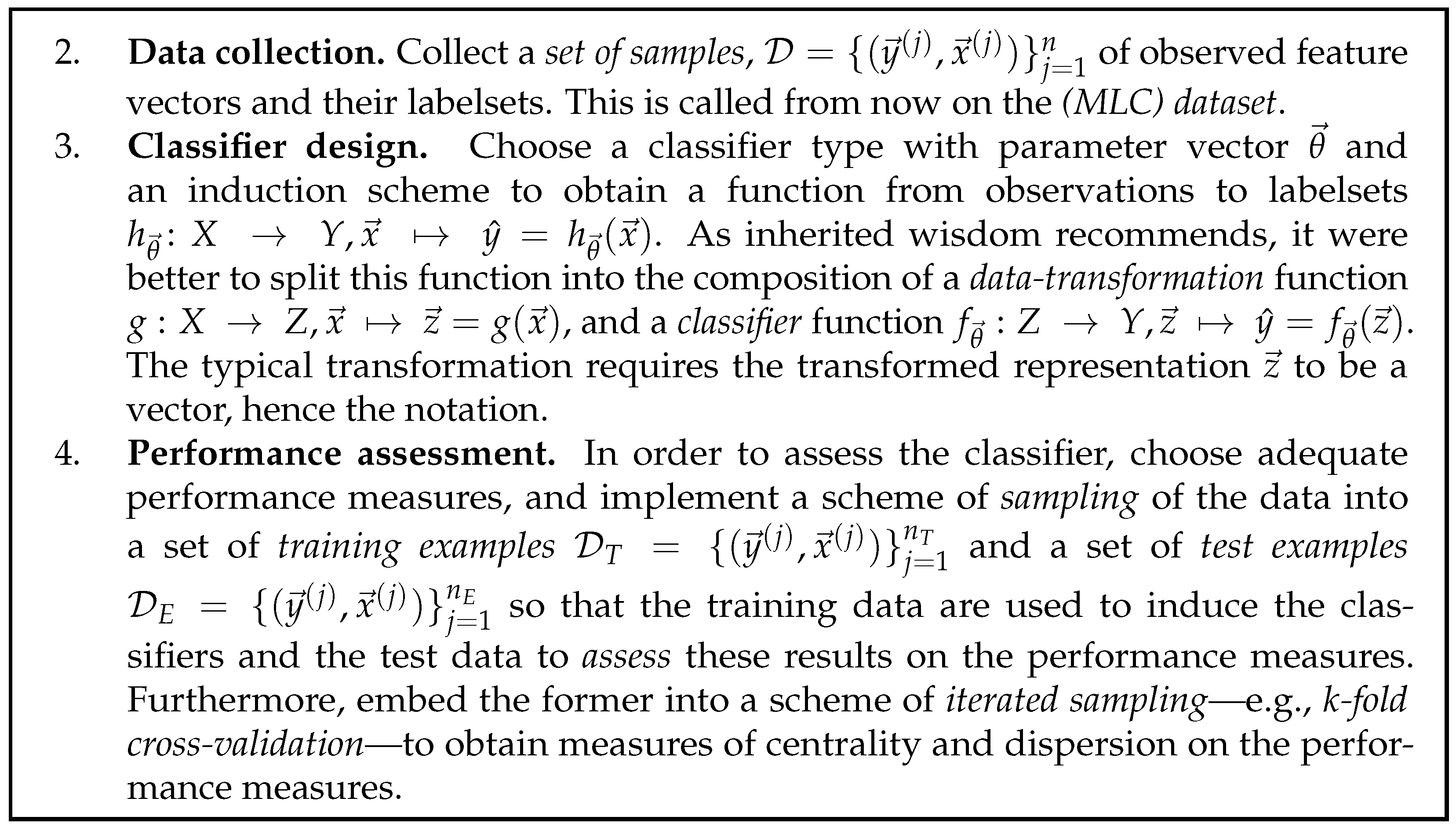
Figure 2. Pseudo-algorithm for MLC under the predictive inference metaphor.
Mathematics 12 00346 g002
Figure 3. Basic scheme for multiclass classification. Y and Y ^ are categorical variables.
Mathematics 12 00346 g003
Figure 4. (Colour online) Extended entropy diagram of a trivariate distribution. The bounding rectangle is the joint entropy of uniform (hence independent) distributions U X i of the same cardinality as distribution P X i . The green area is the sum of the multi-information (total correlation) C P X ¯ and the dual total correlation D P X ¯ . Reprinted from [33], Copyright (2017), with permission from Elsevier.
Mathematics 12 00346 g004
Figure 5. Conceptually annotated Source Multivariate Entropy Triangle (from [33]). Notice that this is valid both for aggregate and individual entropic decomposition with analogue meanings. Reprinted from [33], Copyright (2017), with permission from Elsevier.
Mathematics 12 00346 g005
Figure 6. Reproduction of the example of [34], p. 18, using ConExp. In the lattice, meet irreducibles are half-filled in blue, and join irreducibles in black.
Mathematics 12 00346 g006
Figure 7. Labelling context D L = ( G , L , I ) and its lattice B ̲ ( G , L , I ) for emotions. Observations are formal objects, labels are formal attributes, and label names are abbreviated to their initials in the context representation. Node size is proportional to the cardinal of its extent.
Mathematics 12 00346 g007
Figure 8. Nominal, contra-nominal, and ordinal scales of order 3 (3 labels). Drawing conventions as for Figure 6.
Mathematics 12 00346 g008
Figure 9. Comparison of average information content of nominal, contra-nominal, and ordinal scales for orders ranging in 2 l where l { 1 , 2 , 3 , 4 , 5 , 7 , 8 } . The information content of nominal and contra-nominal scales is the same for identical order, while that of ordinal scales is more nuanced (explanation in the text).
Mathematics 12 00346 g009
Figure 10. Comparison of individual label information content of nominal, contra-nominal, and ordinal scales for orders ranging in 2 l where l { 1 , 2 , 3 , 4 , 5 , 7 , 8 } . For nominal and contra-nominal scales every label has the same information so they lie atop each other in the left-hand side of the triangle. However, labels in ordinal scales lie along a rough line from left to right with increasing order, typically in overlying pairs—a variable and its complementary.
Mathematics 12 00346 g010
Figure 11. Zoomable plot of the average source entropy decomposition of the datasets considered from [25] by cluster, with details of the lowest, almost deterministic zone.
Mathematics 12 00346 g011
Figure 12. Individual (dots) and aggregated (crosshairs) label information content for the selected datasets of Table 2, coloured by cluster. emotions and flags are more similar in appearance, as are, on the one hand, eurlexdc and rcv1sub1, and birds and slashdot, on the other. Perhaps enron is a subclass of its own.
Mathematics 12 00346 g012
Figure 13. SMET for emotions in several thresholds. Colour of the glyphs reflects the square of the threshold value (explanation in the text.)
Mathematics 12 00346 g013
Figure 14. Multisplit SMET for emotions for the ‘angry-aggresive’, ‘quite-still’ and ‘relaxing-calm’ labels with cross-validated entropies, following the guidelines developed in this paper. Test set entropies in red, train in blue. Notice how the entropies of the splits almost overlap.
Mathematics 12 00346 g014
Figure 15. Effect of hapax thresholding on the number of concepts of B ̲ L ( G , L , I ) for emotions.
Mathematics 12 00346 g015
Figure 17. Interim version of MLC under the predictive inference metaphor. Further specifying step 3 is left for future work.
Mathematics 12 00346 g017
Figure 18. Full model for MLC Sources: Y ¯ and Y ^ are a source and a presentation of random vectors of binary variables that can be quantitatively and qualitatively characterized using the entropy coordinates F ( P Y ¯ ) = [ Δ H P Y ¯ , M P Y ¯ , V I P Y ¯ ] —and related SMETs both aggregate and label-wise—and the concept lattice of the labelling context B ̲ ( G , L , I ) , respectively.
Mathematics 12 00346 g018
Table 1. Measurements for some of the datasets in [25]. Only the datasets contained in R packages mldr [26] and mldr.datasets [27] were analysed.
Dataset Name | B L ( G , L , I ) | d | L | n | F |
1flags7954719419
2yeast686198142417103
3ng2058552019,3001006
4emotions3027659372
5scene171562407294
6bookmarks150,33718,71620887,8562150
7delicious9,343,38515,80698316,105500
8enron15957535317021001
9bibtex6298285615973951836
10corel5k570231753745000499
11corel16k0026498486816413,761500
12corel16k0036354481215413,760500
13corel16k0106245469214413,618500
14corel16k0046547486016213,837500
15corel16k0016478480315313,766500
16corel16k0066649500916213,859500
17corel16k0077017515817413,915500
18corel16k0056841503416013,847500
19corel16k0086479495616813,864500
20corel16k0096972517517313,884500
21genbase3932276621186
22tmc2007207213412228,59649,060
23medical9894459781449
24tmc2007_500182011722228,596500
25eurlexev54,47916,467399319,3485000
26eurlexdc1712161541219,3485000
27birds15413319645260
28foodtruck2501161240721
29langlog3373047514601004
30cal5002,560,36550217450268
31mediamill20,013655510143,907120
32stackex_coffee2071741232251763
33stackex_cooking8070638640010,491577
34stackex_cs652847492749270635
35stackex_chess157310782271675585
36stackex_chemistry389030321756961540
37stackex_philosophy316822492333971842
38rcv1sub41429816101600047,229
39rcv1sub120121028101600047,236
40rcv1sub51828946101600047,235
41rcv1sub31645939101600047,236
42rcv1sub21781954101600047,236
43yahoo_reference32727533802739,679
44yahoo_business3352333011,21421,924
45yahoo_social4793613912,11152,350
46yahoo_health51033532920530,605
47yahoo_education6635113312,03027,534
48imdb7273450328120,9191001
49ohsumed133511472313,9291002
50yahoo_recreation11205302212,82830,324
51yahoo_science60145740642837,187
52yahoo_society241810542714,51231,802
53yahoo_entertainment4903372112,73032,001
54reutersk5009568111036000500
55slashdot1591562237821079
56yahoo_arts107159926748423,146
Table 2. A selection of multilabel classification databases by Cluster—from [25]—and Nameflags, emotions(musicout) [57], enron, birds [58] rcv1sub1, and slashdot. | B L ( G , L , I ) | is the size of the lattice of intents of the labelling context, actual refers to the actual count of distinct labelsets in the label context, while | L | is the cardinality of labels, n that of observations, and | F | that of features in each dataset.
ClusterName | B L ( G , L , I ) | Actual | L | n | F |
1flags7954719419
2emotions3027659372
3enron15957535317021001
4eurlexdc1712161541219,3485000
5birds15413319645260
7rcv1sub120121028101600047,236
8slashdot1591562237821079
Disclaimer/Publisher’s Note: The statements, opinions and data contained in all publications are solely those of the individual author(s) and contributor(s) and not of MDPI and/or the editor(s). MDPI and/or the editor(s) disclaim responsibility for any injury to people or property resulting from any ideas, methods, instructions or products referred to in the content.