On Block g-Circulant Matrices with Discrete Cosine and Sine Transforms for Transformer-Based Translation Machine

Abstract

Transformer has emerged as one of the modern neural networks that has been applied in numerous applications. However, transformers’ large and deep architecture makes them computationally and memory-intensive. In this paper, we propose the block g-circulant matrices to replace the dense weight matrices in the feedforward layers of the transformer and leverage the DCT-DST algorithm to multiply these matrices with the input vector. Our test using Portuguese-English datasets shows that the suggested method improves model memory efficiency compared to the dense transformer but at the cost of a slight drop in accuracy. We found that the model Dense-block 1-circulant DCT-DST of 128 dimensions achieved the highest model memory efficiency at 22.14%. We further show that the same model achieved a BLEU score of 26.47%.

1. Introduction

Across a wide range of applications, including chatbots [1], machine translation [2], text summarization [3], video-image processing [4,5,6], etc., transformer neural networks have significantly improved. As demonstrated by [7,8,9,10,11], transformers and their modifications have proven superior, particularly in machine translation. As the amount of computational power required for training and inference increases, one of the more advanced neural networks is the Transformer [12], which has a deeper topology. Conversely, the depth of the transformer architecture gives rise to several constraints and challenges, including high computational complexity [13], substantial demands on computational resources [14], and high memory consumption [15] that quadratic to the input sequence length. Therefore, methods are required to achieve excellent performance, mainly when using them as translation machines. Several approaches have been put forth to address this problem, including weight matrix decomposition, matrix-vector algorithm selection, and weight matrix replacement.

Utilizing a structured weight matrix is considered a crucial tactic among other strategies because of its benefits. According to [16], this may lessen the memory needed for training and storing the model (and optimizer). This alternative approach can also mitigate computational complexity, leveraging the benefits of the selected structured weight matrix [12]. This fact has encouraged the creation of a wide variety of structured matrices, including low-rank matrices [17], Toeplitz-like matrices [18], block-circulant matrices [19,20], fast-food transforms [21], low displacement rank matrices [22], and butterfly matrices [23], among other matrices. One of the Low Displacement Rank (LDR) matrices is the block g-circulant matrix [24,25]. The block g-circulant matrix combines features from block-circulant and g-circulant matrices. Its adoption as a replacement for the transformer weight matrix is believed to enhance transformer performance, building on findings from prior research [26,27]. With a g position shift to the right, this matrix is a generalization of the block circulant matrix. This property makes more intricate patterns and interactions within the matrix possible, expanding the range of potential uses. Among their many benefits is the ability to find efficient algorithms, such as those for multiplying them by any vector to reduce computational complexity [28]. This is why structured matrices are used as transformer weight matrices.

We have found that the Fast Fourier Transform (FFT) algorithm is dependable when the structured matrix is a circulant matrix [29]. The ability of the FFT Transformer to compress model memory up to 100 times has been demonstrated. This transformer is based on the feedforward layer’s block g-circulant weight matrices. Liu [28] discovered the Discrete Cosine Transform-Discrete Sine Transform (DCT-DST) algorithm for circulant matrix-vector products, which can save storage compared to FFT. No text processing system has ever employed the DCT-DST algorithm. Processing photos and videos is its more common usage [30,31]. With a DCT-DST algorithm for the translation machine, we present a novel method for executing a real block g-circulant weight matrix-based transformer in this paper. Our objective is to impose a block g-circulant structure on transformer model topologies through the elegant mathematical characteristic of the block g-circulant matrix. The contributions of this paper are summarized as follows:

• We define the block g-circulant matrix and generate several lemmas and theorems regarding the characteristics and possible eigenvalues, as well as defining the matrices utilized in carrying out the DCT-DST algorithm for multiplication of block g-circulant matrices.
• We propose a new approach in using structured matrices as a replacement for dense weight matrices, combined with matrix multiplication algorithms, in this case, a combination of block g-circulant matrices and the DCT-DST algorithm.
• Our research is the first study that applied the DCT-DST algorithm for weight matrix-vector multiplication in a transformer-based translation machine.

In this article, we present a structured exploration of key concepts. Firstly, we delve into the foundational motivation driving our exploration of block g-circulant matrices and the DCT-DST algorithm. Section 2 explains the theories and characteristics of block g-circulant matrices, including a comprehensive examination of the potential eigenvalues of real block g-circulant matrices. Section 3 describes the workings of the block g-circulant DCT-DST transformer, including a comprehensive explanation of the associated algorithm. Section 4 presents our experimental methodology, results, and a thorough discussion of the research findings. Finally, we summarize our insights in a concise conclusion in the closing section.

2. Block g-Circulant Matrix

Definition 1.

Let $C_i$ be a $m\times m$ matrix for each $i=1,\cdots ,n$. Then a $nm\times nm$ block-circulant matrix $C_{nm}$ is generated from the ordered set $C_1,C_2,\cdots ,C_n$, and is of the form

$$C_{nm}=\left[\begin{array}{cccc}{C}_1& C_2& \cdots & C_n\\ C_n& C_1& \cdots & C_{n-1}\\ ⋮& ⋮& \ddots & ⋮\\ C_2& C_3& \cdots & C_1\end{array}\right].$$

The set of all such matrices of order $nm\times nm$ will be denoted by $B{C}_{nm}$, whereas $B_m$ represents the set of all circulant matrices of dimension m.

Theorem 1

([32]). Let $C_{nm}\in B{C}_{nm}$ has generating elements $C_1,C_2,\cdots ,C_n\in B_m$. If $c_i^{\left(1\right)}$, $c_i^{\left(2\right)},\cdots ,c_i^{\left(m\right)}$ are generating elements of $C_i$, then

$$(F_n^{\ast }\otimes F_m^{\ast })C_{nm}(F_n\otimes F_m)=D_{nm}=dia{g}_{i=1,\cdots ,n}\left[\begin{array}{cccc}{\lambda }_i^{\left(1\right)}& 0& \cdots & 0\\ 0& {\lambda }_i^{\left(2\right)}& \cdots & 0\\ ⋮& ⋮& \ddots & ⋮\\ 0& 0& \cdots & {\lambda }_i^{\left(m\right)}\end{array}\right]$$

(1)

is a diagonal matrix of dimension $nm\times nm$ with

$${\lambda }_i^{\left(p\right)}=\sum _{k=1}^n\sum _{l=1}^m{c}_k^l{\omega }_{p-1}^{l-1}{\omega }_{i-1}^{k-1},$$

(2)

with $i=1,2,\cdots ,n$ and $p=1,2,\cdots ,m.$

$$F_n=\frac{1}{\sqrt{n}}{\omega }^{-jk},j,k=0,1,\cdots ,n-1$$

(3)

with $\omega =e^{\frac{2\pi }{n}i},i=\sqrt{-1}$.

In case $C_{nm}\in {\mathbb{R}}^{nm\times nm}$, we can decompose the diagonalization of $C_{nm}$ [26] as follow:

$$(U_n^{\ast }\otimes U_m^{\ast })C_{nm}(U_n\otimes U_m)={\Omega }_{nm}$$

(4)

with

$$U_n=\left\{\begin{array}{cc}\left[t_0,\sqrt{2}{t}_1,\cdots ,\sqrt{2}{t}_{h-1},t_h,\sqrt{2}{s}_{h-1},\cdots ,\sqrt{2}{s}_1\right],\hfill & \mathrm{if}n=2h\hfill \\ \left[t_0,\sqrt{2}{t}_1,\cdots ,\sqrt{2}{t}_h,\sqrt{2}{s}_h,\cdots ,\sqrt{2}{s}_1\right],\hfill & \mathrm{if}n=2h+1\hfill \end{array}\right.$$

(5)

where $t_k$ and $s_k$ are real and imaginary parts of columns of $F_n=[f_0,f_1,\cdots ,f_h]$ and

$${\Omega }_{nm}=\left[\begin{array}{cccccccc}\hfill q_1& & & & & & & \\ \hfill & q_2& & & & & & s_2\\ & & \ddots \hfill & & & & ⋰& \\ & & & q_h& & s_h& & \\ \hfill & & & & q_{h+1}& & & \\ \hfill & & & -s_h& & q_h& & \\ & & ⋰\hfill & & & & \ddots & \\ & -s_2& & & & & & q_2\end{array}\right]$$

and for $n=2h+1$ it will be

$${\Omega }_{nm}=\left[\begin{array}{ccccccc}\hfill q_1& & & & & & \\ \hfill & q_2& & & & & s_2\\ & & \ddots \hfill & & & ⋰& \\ & & & q_{h+1}& s_{h+1}& & \\ \hfill & & & -s_{h+1}& q_{h+1}& & \\ & & ⋰\hfill & & & \ddots & \\ & -s_2& & & & & q_2\end{array}\right]$$

with

$$\begin{array}{c}\hfill q_i=\left\{\begin{array}{cc}\left[\begin{array}{cccccccc}\hfill \sum _{k=1}^n{a}_k^{\left(i\right)}{\alpha }_k^{\left(1\right)}& & & & & & & \\ \hfill & \sum _{k=1}^n{a}_k^{\left(i\right)}{\alpha }_k^{\left(2\right)}& \hfill & & & & & \sum _{k=1}^n{a}_k^{\left(i\right)}{\beta }_k^{\left(2\right)}\\ \hfill & & \ddots \hfill & & & & ⋰& \\ \hfill & & & \sum _{k=1}^n{a}_k^{\left(i\right)}{\alpha }_k^{\left(r\right)}& & \sum _{k=1}^n{a}_k^{\left(i\right)}{\beta }_k^{\left(r\right)}& & \\ \hfill & & & & \sum _{k=1}^n{a}_k^{\left(i\right)}{\alpha }_k^{(r+1)}& & & \\ \hfill & & & -\sum _{k=1}^n{a}_k^{\left(i\right)}{\beta }_k^{\left(r\right)}& & \sum _{k=1}^n{a}_k^{\left(i\right)}{\alpha }_k^{\left(r\right)}& & \\ \hfill & & ⋰\hfill & & & & \ddots & \\ \hfill & -\sum _{k=1}^n{a}_k^{\left(i\right)}{\beta }_k^{\left(2\right)}& \hfill & & & & & -\sum _{k=1}^n{a}_k^{\left(i\right)}{\beta }_k^{\left(2\right)}\end{array}\right],\hfill & \mathrm{if}m=2r\hfill \\ \\ \left[\begin{array}{ccccccc}\hfill \sum _{k=1}^n{a}_k^{\left(i\right)}{\alpha }_k^{\left(1\right)}& & & & & & \\ \hfill & \sum _{k=1}^n{a}_k^{\left(i\right)}{\alpha }_k^{\left(2\right)}& \hfill & & & & \sum _{k=1}^n{a}_k^{\left(i\right)}{\beta }_k^{\left(2\right)}\\ \hfill & & \ddots \hfill & & & ⋰& \\ \hfill & & & \sum _{k=1}^n{a}_k^{\left(i\right)}{\alpha }_k^{(r+1)}& \sum _{k=1}^n{a}_k^{\left(i\right)}{\beta }_k^{(r+1)}& & \\ \hfill & & & -\sum _{k=1}^n{a}_k^{\left(i\right)}{\beta }_k^{(r+1)}& \sum _{k=1}^n{a}_k^{\left(i\right)}{\alpha }_k^{(r+1)}& & \\ \hfill & & ⋰\hfill & & & \ddots & \\ \hfill & -\sum _{k=1}^n{a}_k^{\left(i\right)}{\beta }_k^{\left(2\right)}& \hfill & & & & \sum _{k=1}^n{a}_k^{\left(i\right)}{\alpha }_k^{\left(2\right)}\end{array}\right],\hfill & \mathrm{if}m=2r+1\hfill \end{array}\right.\end{array}$$

and

$$\begin{array}{c}\hfill s_i=\left\{\begin{array}{cc}\left[\begin{array}{cccccccc}\hfill \sum _{k=1}^n{b}_k^{\left(i\right)}{\alpha }_k^{\left(1\right)}& & & & & & & \\ \hfill & \sum _{k=1}^n{b}_k^{\left(i\right)}{\alpha }_k^{\left(2\right)}& \hfill & & & & & \sum _{k=1}^n{b}_k^{\left(i\right)}{\beta }_k^{\left(2\right)}\\ \hfill & & \ddots \hfill & & & & ⋰& \\ \hfill & & & \sum _{k=1}^n{b}_k^{\left(i\right)}{\alpha }_k^{\left(r\right)}& & \sum _{k=1}^n{b}_k^{\left(i\right)}{\beta }_k^{\left(r\right)}& & \\ \hfill & & & & \sum _{k=1}^n{b}_k^{\left(i\right)}{\alpha }_k^{(r+1)}& & & \\ \hfill & & & -\sum _{k=1}^n{b}_k^{\left(i\right)}{\beta }_k^{\left(r\right)}& & \sum _{k=1}^n{b}_k^{\left(i\right)}{\alpha }_k^{\left(r\right)}& & \\ \hfill & & ⋰\hfill & & & & \ddots & \\ \hfill & -\sum _{k=1}^n{b}_k^{\left(i\right)}{\beta }_k^{\left(2\right)}& \hfill & & & & & -\sum _{k=1}^n{b}_k^{\left(i\right)}{\beta }_k^{\left(2\right)}\end{array}\right],\hfill & \mathrm{if}m=2r\hfill \\ \\ \left[\begin{array}{ccccccc}\hfill \sum _{k=1}^n{b}_k^{\left(i\right)}{\alpha }_k^{\left(1\right)}& & & & & & \\ \hfill & \sum _{k=1}^n{b}_k^{\left(i\right)}{\alpha }_k^{\left(2\right)}& \hfill & & & & \sum _{k=1}^n{b}_k^{\left(i\right)}{\beta }_k^{\left(2\right)}\\ \hfill & & \ddots \hfill & & & ⋰& \\ \hfill & & & \sum _{k=1}^n{b}_k^{\left(i\right)}{\alpha }_k^{(r+1)}& \sum _{k=1}^n{b}_k^{\left(i\right)}{\beta }_k^{(r+1)}& & \\ \hfill & & & -\sum _{k=1}^n{b}_k^{\left(i\right)}{\beta }_k^{(r+1)}& \sum _{k=1}^n{b}_k^{\left(i\right)}{\alpha }_k^{(r+1)}& & \\ \hfill & & ⋰\hfill & & & \ddots & \\ \hfill & -\sum _{k=1}^n{b}_k^{\left(i\right)}{\beta }_k^{\left(2\right)}& \hfill & & & & \sum _{k=1}^n{b}_k^{\left(i\right)}{\alpha }_k^{\left(2\right)}\end{array}\right],\hfill & \mathrm{if}m=2r+1\hfill \end{array}\right.\end{array}$$

where $\alpha ,\beta$, and $a,b$ denote a real and imaginary part of the eigenvalues of $C_{nm}$ decomposers.

Definition 2

([28]). The Discrete Cosine Transform (DCT) I and V matrices are defined as follows

$${\mathcal{C}}_{n+1}^I=\sqrt{\frac{2}{n}}{\left[{\tau }_j{\tau }_{k}cos\frac{jk\pi }{n}\right]}_{j,k=0}^n$$

(6)

$${\mathcal{C}}_n^V=\frac{2}{\sqrt{2n-1}}{\left[{\tau }_j{\tau }_{k}cos\frac{2jk\pi }{2n-1}\right]}_{j,k=0}^{n-1}$$

(7)

$\begin{array}{l}\mathit{with}{\tau }_{l(l=j,k)}=\left\{\begin{array}{cc}\frac{1}{\sqrt{2}},\hfill & if l=0 or l=n\hfill \\ 1,\hfill & if l otherwise\hfill \end{array}\right.\\ {\iota }_k=\left\{\begin{array}{cc}\frac{1}{\sqrt{2}},\hfill & ifk=n-1\hfill \\ 1,\hfill & if k otherwise\hfill \end{array}\right.\end{array}$

Definition 3

([28]). The Discrete Sine Transform (DST) I and V matrices are defined as follows

$${\mathcal{S}}_{n-1}^I=\sqrt{\frac{2}{n}}{\left[sin\frac{jk\pi }{n}\right]}_{j,k=1}^{n-1}$$

(8)

$${\mathcal{S}}_{n-1}^V=\frac{2}{\sqrt{2n-1}}{\left[sin\frac{2jk\pi }{2n-1}\right]}_{j,k=1}^{n-1}$$

(9)

In the following theorem, we will see that the matrix $U_n$, defined in (5), can be partitioned into a matrix generated by the DCT-DST matrices.

Theorem 2

([28]). Let $U_n$ be the matrix stated in (5). Then $U_n$ can be partitioned into the following form

$$U_n=\left\{\begin{array}{cc}\left[\begin{array}{cc}{\sigma }_1{q}_{h+1}^T& 0\\ \mathcal{C}& -\frac{1}{2}\sqrt{2}{\mathcal{S}}_{h-1}^I{J}_{h-1}\\ {\sigma }_1{v}_{h+1}^T& 0\\ J_{h-1}\mathcal{C}& \frac{1}{2}\sqrt{2}{J}_{h-1}{\mathcal{S}}_{h-1}^I{J}_{h-1}\end{array}\right],\hfill & ifn=2h\hfill \\ \\ \left[\begin{array}{cc}{\sigma }_1{p}_{h+1}^T& 0\\ \mathcal{C}& -\frac{1}{2}\sqrt{2}{\mathcal{S}}_h^V{J}_h\\ J_h\mathcal{C}& \frac{1}{2}\sqrt{2}{J}_h{\mathcal{S}}_h^V{J}_h\end{array}\right],\hfill & ifn=2h+1\hfill \end{array}\right.$$

(10)

Definition 4.

Let $C_i^{\left(p\right)}$ be a $m\times m$ g-circulant matrix, i.e., classical circulant matrix with each row shifted g position to the right. A $nm\times nm$ matrix $C_{nmg}$ is a block g-circulant matrix if it is generated by $C_i^{\left(p\right)}$, $i=1,2,\cdots ,n$; $p=1,2,\cdots ,m$ and shifted g position to the right.

Lemma 1.

Let $C_{nmg}\in {\mathbb{C}}^{nm\times nm}$ be a block g-circulant matrix with n block, and each block has order m. Then $C_{nmg}$ can be denoted as

$$C_{nmg}=Z_{nmg}{C}_{nm}$$

(11)

where $C_{nm}$ is a block g-circulant matrix with $g=1$ and

$$Z_{nmg}=Z_{n,g}\otimes Z_{m,g}$$

(12)

where

$$Z_{n,g}={\left[{\delta }_{(gr-s)modn}\right]}_{g,r=0}^{n-1}$$

(13)

$${\delta }_k=\left\{\begin{array}{c}1ifk\equiv 0modn\hfill \\ 0ifkotherwise\hfill \end{array}\right.$$

(14)

and by (1) we have

$$C_{nmg}=Z_{nmg}(F_n\otimes F_m)D_{nm}(F_n^{\ast }\otimes F_m^{\ast })$$

(15)

Lemma 2.

Let $n,m\in \mathbb{Z}$ and $n,m>2$., and let $n_g=n/(n,g)$, $m_g=m/(m,g)$ with $(n,g)$ and $(m,g)$ are the great common divisor between n, m respectively with g. Then we have

$$\begin{array}{cc}{Z}_{nmg}=& \underbrace{{\left[\begin{array}{c}{\tilde{Z}}_{nmg}|{\tilde{Z}}_{nmg}|\cdots |{\tilde{Z}}_{nmg}\end{array}\right]}^T}\\ & (n,g)\times (m,g) \mathit{times}\end{array}$$

(16)

where $Z_{nmg}$ is the matrix defined in (12) and ${\tilde{Z}}_{nmg}\in {\mathbb{C}}^{(n_g\times m_g)\times nm}$ is the submatrix of $Z_{nmg}$ obtained by considering only its first $(n_g\times m_g)$ rows.

Lemma 3

([33]). Let $g\ge n$, then

(a) 

$Z_{n,g}=Z_{n,g^o}$,

(b) 

${\mathbb{C}}_{n,g}={\mathbb{C}}_{n,g^o}$,

(c) 

$M_{n,g}=M_{n,g^o}$

(d) 

$M_{n,g}{M}_{n,h}=M_{n,gh}$

where $g^o\equiv g$ mod n.

Lemma 4.

Let $Z_{n,g}$ be the matrix defined ini (13) and $F_n$ be the Fourier matrix defined in (3). Then we have

$$Z_{n,g}=F_n{M}_{n,g}{F}_n^{\ast }$$

(17)

where

$$M_{n,g}={\left[{\delta }_{r-gc}\right]}_{r,c=0}^{n-1}$$

(18)

and ${\delta }_k$ is defined as in (14).

Lemma 5.

Let $g\ge n,m$. Then $Z_{nmg}=Z_{nm{g}^o}$ where $g^o=g$ mod $\left(nm\right)$. As a consequence we have $C_{nmg}=C_{nm{g}^o}$.

Proof. 

From (12) and by Lemma (3), we have that

$$Z_{nmg}=Z_{n,g}\otimes Z_{m,g}=Z_{n,g^o}\otimes Z_{m,g^o}=Z_{nm{g}^o}$$

(19)

and so from (11) we have the equality $C_{nmg}=Z_{nmg}{C}_{nm}=Z_{nm{g}^o}{C}_{nm}=C_{nm{g}^o}$. □

Lemma 6.

Let $Z_{nmg}$ be the matrix defined in (12) and let $F_n$ as defined in (3). Then

$$Z_{nmg}=(F_n\otimes F_m)M_{nmg}(F_n^{\ast }\otimes F_m^{\ast })$$

(20)

where

$$M_{nmg}=M_{n,g}\otimes M_{m,g}={\left[{\delta }_{r-gs}\right]}_{r,s=0}^{n-1}\otimes {\left[{\delta }_{r-gs}\right]}_{r,s=0}^{m-1}.$$

(21)

and ${\delta }_k$ is defined as in (14).

Proof. 

It suffices to show that $(F_n^{\ast }\otimes F_m^{\ast })Z_{nmg}=M_{mng}(F_n^{\ast }\otimes F_m^{\ast })$.

Using (12), kronecker product properties, and (17) we have

$$\begin{array}{cc}\hfill (F_n^{\ast }\otimes F_m^{\ast })Z_{nmg}& =(F_n^{\ast }\otimes F_m^{\ast })(Z_{n,g}\otimes Z_{m,g})\hfill \\ \hfill & =F_n^{\ast }{Z}_{n,g}\otimes F_m^{\ast }{Z}_{m,g}\hfill \\ \hfill & =M_{n,g}{F}_n^{\ast }\otimes M_{m,g}{F}_m^{\ast }\hfill \\ \hfill & =(M_{n,g}\otimes M_{m,g})(F_n^{\ast }\otimes F_m^{\ast })\hfill \\ \hfill & =M_{nmg}(F_n^{\ast }\otimes F_m^{\ast }).\hfill \end{array}$$

□

In the following lemma, we will see that Lemma (5) also holds for the matrix $M_{mng}$.

Lemma 7.

If $g\ge n,m$, then $M_{nmg}=M_{nm{g}^o}$ with $g^o=g$ mod $\left(nm\right)$.

Proof. 

By using (20) we have

$$\begin{array}{c}\hfill Z_{nmg}=(F_n\otimes F_m)M_{nmg}(F_n^{\ast }\otimes F_m^{\ast })\\ \hfill Z_{nm{g}^o}=(F_n\otimes F_m)M_{nm{g}^o}(F_n^{\ast }\otimes F_m^{\ast })\end{array}$$

By Lemma (5), we deduce

$$(F_n\otimes F_m)M_{nmg}(F_n^{\ast }\otimes F_m^{\ast })=(F_n\otimes F_m)M_{nm{g}^o}(F_n^{\ast }\otimes F_m^{\ast })$$

and so $M_{nmg}=M_{nm{g}^o}$. □

Lemma 8.

Let $D_{nm}\in {\mathbb{C}}^{nm\times nm}$ be a diagonal matrix

$$D_{nm}=\underset{\begin{array}{c}p=0,\cdots ,m-1\\ j=0,\cdots ,n-1\end{array}}{\mathrm{diag}}\left({\lambda }_j^{\left(p\right)}\right)$$

where $p=0,\cdots ,m-1;j=0,\cdots ,n-1$, and let $M_{nmg}$ be the matrix defined in (21). Then

$$D_{nm}{M}_{nmg}=M_{nmg}{\tilde{D}}_{nmg}$$

(22)

where ${\tilde{D}}_{nmg}=\underset{\begin{array}{c}p=0,\cdots ,m-1\\ j=0,\cdots ,n-1\end{array}}{\mathrm{diag}}\left({\lambda }_{gj\left(modn\right)}^{\left(gp\right(modn\left)\right)}\right)$.

Lemma 9.

Let $C_{nmg}\in {\mathbb{C}}^{nm\times nm}$ be a g-block circulant matrix and $C_{nmh}\in {\mathbb{C}}^{nm\times nm}$ be a h-block circulant matrix. Then $C_{nmg}{C}_{nmh}\in {\mathbb{C}}^{nm\times nm}$ is a $gh$-block circulant matrix.

Proof. 

Using (11) and (15) we have

$$C_{nmg}=Z_{nmg}{C}_{nm}=Z_{nmg}(F_n\otimes F_m)D_{nm}^{\left(1\right)}(F_n^{\ast }\otimes F_m^{\ast })$$

and

$$C_{nmh}=Z_{nmh}{C}_{nm}=Z_{nmh}(F_n\otimes F_m)D_{nm}^{\left(2\right)}(F_n^{\ast }\otimes F_m^{\ast }).$$

Since (20), then

$$C_{nmg}{C}_{nmh}=(F_n\otimes F_m)M_{nmg}{D}_{nm}^{\left(1\right)}{M}_{nmh}{D}_{nm}^{\left(2\right)}(F_n^{\ast }\otimes F_m^{\ast })$$

By using (22), the last equation will be

$$C_{nmg}{C}_{nmh}=(F_n\otimes F_m)M_{nmg}{M}_{nmh}{\tilde{D}}_{nmg}^{\left(1\right)}{D}_{nm}^{\left(2\right)}(F_n^{\ast }\otimes F_m^{\ast })$$

Furthermore by (21) and Kronecker product properties we have

$$\begin{array}{cc}\hfill M_{nmg}{M}_{nmh}& =(M_{ng}\otimes M_{mg})(M_{nh}\otimes M_{mh})\hfill \end{array}$$

(23)

$$\begin{array}{cc}\hfill & =\left(M_{ng}{M}_{nh}\right)\otimes \left(M_{mg}{M}_{mh}\right)\hfill \end{array}$$

(24)

$$\begin{array}{cc}\hfill & =\left(M_{ngh}\right)\otimes \left(M_{mgh}\right)\hfill \end{array}$$

(25)

$$\begin{array}{c}=M_{nmgh}\hfill \end{array}$$

(26)

So by (20) we obtain

$$C_{nmg}{C}_{nmh}=Z_{nmgh}(F_n\otimes F_m){\tilde{D}}_{nmg}^{\left(1\right)}{D}_{nm}^{\left(2\right)}(F_n^{\ast }\otimes F_m^{\ast })$$

Since ${\tilde{D}}_{nmg}^{\left(1\right)}{D}_{nm}^{\left(2\right)}$ is a diagonal matrix, then the last equation is the representation of $gh$-circulant. □

2.1. Eigenvalues of Block g-Circulant Matrices

In this section, we explore the eigenvalues of a block g-circulant matrix in case $g=0,g=1$, and $(n,g)\ne 1$ and $(m,g)\ne 1$.

2.1.1. Case $g=0$

If $g=0$, this means that $C_{nmg}$ is a matrix that has constant elements along all the rows in each block and, therefore, it has rank 1; then, remembering that the trace (tr(·)) of a matrix is the sum of its eigenvalues, we can conclude that $C_{nmg}$ has $(nm\times nm)-1$ zero eigenvalues and one eigenvalue $\lambda$ different from zero given by

$$\lambda \left(C_{nmg}\right)=\sum _{i=1}^{n}tr\left(C_i\right)=\sum _{i=1}^n\sum _{p=1}^m{c}_i^{\left(p\right)}$$

where $C_i=(c_i^{\left(1\right)},c_i^{\left(2\right)},\cdots ,c_i^{\left(m\right)})$ and $c_i^{\left(p\right)}$ is the entry of the ith block and pth column.

2.1.2. Case $g=1$

If $g=1$, then the $C_{nmg}$ is a “classical” block circulant matrix as defined in Definition 1, and its eigenvalues are given by

$${\lambda }_i^{\left(p\right)}=\sum _{k=1}^n\sum _{l=1}^m{c}_k^l{\omega }_{p-1}^{l-1}{\omega }_{i-1}^{k-1}$$

(27)

2.1.3. Case $(nm,g)\ne 1$

The following theorem we will use to calculate the eigenvalues of a singular matrix $A\in {\mathbb{C}}^{n\times n}$ with rank $\left(A\right)=r\le n$ by calculating the eigenvalues of a smaller matrix $A\in {\mathbb{C}}^{k\times k}$ with $r\le k\le n$.

Theorem 3

([34]). Let A be a matrix of dimension $n\times n$, $A\in {\mathbb{C}}^{n\times n}$, which can be written as $A=X{Y}^{\ast }$, where $X,Y\in {\mathbb{C}}^{n\times k}$, with $k\le n$. Then the eigenvalues of the matrix A are given by k eigenvalues of the matrix $Y^{\ast }X\in {\mathbb{C}}^{k\times k}$ and $n-k$ zero eigenvalues:

$$Eig\left(A\right)=Eig\left(Y^{\ast }X\right)\bigcup \{0withgeometricmultiplicityn-k\}.$$

We will apply Theorem (3) while considering that the matrix $C_{nmg}$ is singular. By Lemma 2 we can write that

$$\begin{array}{cc}\hfill Z_{nmg}& ={\left[\begin{array}{c}{\tilde{Z}}_{nmg}|{\tilde{Z}}_{nmg}|\cdots |{\tilde{Z}}_{nmg}\end{array}\right]}^T\hfill \\ \hfill & =\left({\left[\begin{array}{c}{I}_{n_g}|I_{n_g}|\cdots |I_{n_g}\end{array}\right]}^T\otimes {\left[\begin{array}{c}{I}_{m_g}|I_{m_g}|\cdots |I_{m_g}\end{array}\right]}^T\right)({\tilde{Z}}_{n,g}\otimes {\tilde{Z}}_{m,g})\hfill \\ \hfill & =I_{n{m}_g}{\tilde{Z}}_{nmg}\hfill \end{array}$$

where ${\tilde{Z}}_{nmg}\in {\mathbb{C}}^{(n_g\times m_g)\times nm}$ and $I_{n{m}_g}$ is the identity matrix of dimension $nm\times (n_g\times m_g)$. Now we can rewrite (11) as bellow

$$\begin{array}{cc}\hfill C_{nmg}& =Z_{nmg}{C}_{nm}\hfill \\ \hfill & =I_{n{m}_g}{\tilde{Z}}_{nmg}{C}_{nm}\hfill \\ \hfill & =I_{n{m}_g}{\tilde{C}}_{nmg}\hfill \end{array}$$

where ${\tilde{C}}_{nmg}={\tilde{Z}}_{nmg}{C}_{nm}\in {\mathbb{C}}^{(n_g\times m_g)\times nm}$.

By Theorem (3) we find that the eigenvalues of $C_{nmg}$ are equal to those of ${\tilde{C}}_{nmg}{I}_{n{m}_g}\in {\mathbb{C}}^{(n_g\times m_g)\times (n_g\times m_g)}$, plus $(nm-(n_g\times m_g))$ null eigenvalues:

$Eig\left(C_{nmg}\right)=Eig\left({\tilde{C}}_{nmg}{I}_{n{m}_g}\right)\bigcup \{0$ with geometric multiplicity $nm-(n_g\times m_g)\}$.

2.1.4. Case $(nm,g)=1$

When both $nm$ and g are coprime, the lemma provides a straightforward formula to compute the modulus of eigenvalues for a g-circulant matrix $C_{nmg}$. This method draws upon the classical eigenvalue computation for the circulant matrix $C_{nm}$.

Lemma 10.

Let $C_{nmg}\in {\mathbb{C}}^{nm\times nm}$ be a g-block circulant such that $(nm,g)=1$ and denote

$$C_{nmg}=Z_{nmg}(F_n^{\ast }\otimes F_m^{\ast })D_{nm}(F_n\otimes F_m)$$

with

$$D_{nm}=\underset{\begin{array}{c}p=0,\cdots ,m-1\\ j=0,\cdots ,n-1\end{array}}{\mathrm{diag}}\left({\lambda }_j^{\left(p\right)}\right)$$

Then, the modulus of the eigenvalues of $C_{nmg}$ are given by

$$|{\lambda }_j^{\left(p\right)}\left(C_{nmg}\right)|=\left|\sqrt[s]{\prod _{k=0}^{s-1}{\lambda }_{\left(g^{k}j\right)modn}^{\left(g^{k}p\right)modm}}\right|,$$

(28)

with $j=0,1,\cdots ,n-1$ and $p=0,1,\cdots ,m-1$. where $s\in {\mathbb{N}}^{+}$ is such that $g^s\equiv 1\left(modn\right)$.

Proof. 

By Lemma (9) we have that if $C_{nmg}$ is a g-block circulant matrix, then $C_{nmg}^r$ is a $g^r$-block circulant matrix, $r\in {\mathbb{Z}}^{+}$. By Lemma (5) $C_{nmg}^r$ is also a ${\tilde{g}}^r$-block circulant matrix, where ${\tilde{g}}^r\equiv g^{r}mod\left(nm\right)$. Since $(nm,g)=1$ then there is $s\in {\mathbb{Z}}^{+}$ such that $g^s\left(modnm\right)\equiv 1$, then $C_{nmg}^s$ is a block circulant matrix. Notice that the eigenvalues of $C_{nmg}$ are the modulus of the roots of index s of the eigenvalues of the block circulant matrix $C_{nmg}^s$. From Equations (15) and (20) we obtain that

$$C_{nmg}^s=(F_n\otimes F_m){\left(M_{nmg{D}_{nm}}\right)}^s(F_n^{\ast }\otimes F_m^{\ast })$$

Since $(F_n\otimes F_m)(F_n^{\ast }\otimes F_m^{\ast })=I$, we have

$$Eig\left(C_{nmg}^s\right)=Eig\left({\left(M_{nmg}{D}_{nm}\right)}^s\right)$$

Using Equation (22) and the fact that $D_{nm}={\tilde{D}}_{nm{g}^o}$, we obtain

$$\begin{array}{cc}\hfill {\left(M_{nmg}{D}_{nm}\right)}^s& =M_{nmg}{D}_{nm}{M}_{nmg}{D}_{nm}.\cdots M_{nmg}{D}_{nm}\hfill \\ \hfill & =M_{nmg}{\left(D_{nm}{M}_{nmg}\right)}^{s-1}{D}_{nm}\hfill \\ \hfill & =M_{nmg}{\left(M_{nmg}{\tilde{D}}_{nmg}\right)}^{s-1}{\tilde{D}}_{nm{g}^o}\hfill \\ \hfill & =M_{nmg}{\left[M_{nmg}\underset{\begin{array}{c}p=0,\cdots ,m-1\\ j=0,\cdots ,n-1\end{array}}{\mathrm{diag}}\left({\lambda }_{\left(gj\right)modn}^{\left(gp\right)modm}\right)\right]}^{s-1}{\tilde{D}}_{nm{g}^o}\hfill \\ \hfill & =M_{nmg}{M}_{nmg}{\left[\underset{\begin{array}{c}p=0,\cdots ,m-1\\ j=0,\cdots ,n-1\end{array}}{\mathrm{diag}}\left({\lambda }_{\left(gj\right)modn}^{\left(gp\right)modm}\right)M_{nmg}\right]}^{s-2}\underset{\begin{array}{c}p=0,\cdots ,m-1\\ j=0,\cdots ,n-1\end{array}}{\mathrm{diag}}\left({\lambda }_{\left(gj\right)modn}^{\left(gp\right)modm}\right){\tilde{D}}_{nm{g}^o}\hfill \\ \hfill & =M_{nmg}^2{\left[\underset{\begin{array}{c}p=0,\cdots ,m-1\\ j=0,\cdots ,n-1\end{array}}{\mathrm{diag}}\left({\lambda }_{\left(gj\right)modn}^{\left(gp\right)modm}\right)M_{nmg}\right]}^{s-2}\underset{\begin{array}{c}p=0,\cdots ,m-1\\ j=0,\cdots ,n-1\end{array}}{\mathrm{diag}}\left({\lambda }_{\left(gj\right)modn}^{\left(gp\right)modm}\right){\tilde{D}}_{nm{g}^o}\hfill \\ \hfill & =M_{nmg}^2{\left[M_{nmg}\underset{\begin{array}{c}p=0,\cdots ,m-1\\ j=0,\cdots ,n-1\end{array}}{\mathrm{diag}}\left({\lambda }_{g\left(gj\right)modn}^{g\left(gp\right)modm}\right)\right]}^{s-2}\underset{\begin{array}{c}p=0,\cdots ,m-1\\ j=0,\cdots ,n-1\end{array}}{\mathrm{diag}}\left({\lambda }_{\left(gj\right)modn}^{\left(gp\right)modm}\right){\tilde{D}}_{nm{g}^o}\hfill \\ \hfill & =M_{nmg}^2{\left[M_{nmg}\underset{\begin{array}{c}p=0,\cdots ,m-1\\ j=0,\cdots ,n-1\end{array}}{\mathrm{diag}}\left({\lambda }_{\left(g^{2}j\right)modn}^{\left(g^{2}p\right)modm}\right)\right]}^{s-2}{\tilde{D}}_{nmg}{\tilde{D}}_{nm{g}^o}\hfill \\ \hfill & =M_{nmg}^3{\left[\underset{\begin{array}{c}p=0,\cdots ,m-1\\ j=0,\cdots ,n-1\end{array}}{\mathrm{diag}}\left({\lambda }_{\left(g^{2}j\right)modn}^{\left(g^{2}p\right)modm}\right)M_{nmg}\right]}^{s-3}\underset{\begin{array}{c}p=0,\cdots ,m-1\\ j=0,\cdots ,n-1\end{array}}{\mathrm{diag}}\left({\lambda }_{\left(g^{2}j\right)modn}^{\left(g^{2}p\right)modm}\right){\tilde{D}}_{nmg}{\tilde{D}}_{nm{g}^o}\hfill \\ \hfill & ⋮\hfill \\ \hfill & =M_{nmg}^s.{\tilde{D}}_{nm{g}^{s-1}}.\cdots {\tilde{D}}_{nm{g}^2}{\tilde{D}}_{nmg}{\tilde{D}}_{nm{g}^o}.\hfill \end{array}$$

Using Lemma (9), Equation (2), and since $g^{s}mod\left(nm\right)\equiv 1$, we have

$$\begin{array}{cc}\hfill M_{nmg}^s& =M_{nmg}.M_{nmg}.\cdots .M_{nmg}\hfill \\ \hfill & =M_{nm{g}^s}=M_{nm{g}^{s}mod\left(nm\right)}=M_{nm}=I_{nm}.\hfill \end{array}$$

Hence, we have that ${\left(M_{nmg}{D}_{nm}\right)}^s$ is a diagonal matrix, and its eigenvalues are given by the diagonal elements of ${\tilde{D}}_{nm{g}^{s-1}}\cdots {\tilde{D}}_{nm{g}^2}{\tilde{D}}_{nmg}{\tilde{D}}_{nm{g}^o}$, i.e., from (22)

$$\begin{array}{cc}\hfill {\lambda }_j^{\left(p\right)}{\left(M_{nmg}{D}_{nm}\right)}^s& =\left({\lambda }_{g^{s-1}jmodn}^{g^{s-1}pmodm}\right)\cdots \left({\lambda }_{g^{2}jmodn}^{g^{2}pmodm}\right)\left({\lambda }_{gjmodn}^{gpmodm}\right)\left({\lambda }_{g^{0}jmodn}^{g^{0}pmodm}\right)\hfill \\ \hfill & =\prod _{k=0}^{s-1}{\lambda }_{\left(g^{k}j\right)modn}^{\left(g^{k}p\right)modm}\hfill \end{array}$$

with $p=0,\cdots ,m-1$ and $j=0,\cdots ,n-1$. So we have the modulus of the eigenvalues of $C_{nmg}$ are the modulus of the roots of index s of the eigenvalues of the block circulant matrix $C_{nmg}^s$. □

Next, we will see a real block g-circulant matrix decomposition into an orthogonal matrix $U_{nmg}$. We also will define an orthogonal matrix $Q_{nmg}$ whose multiplication by $U_{nmg}$ will be used in the DCT-DST algorithm.

Theorem 4.

Let $C_{nmg}\in {\mathbb{R}}^{nm\times nm}$ be a real block g-circulant matrix, and define $U_{nmg}\in {\mathbb{R}}^{nm\times nm}$ as:

$$U_{nmg}=(U_n\otimes U_m)(P_{n,n-g+1}\otimes P_{m,m-g+1})$$

(29)

where $U_t$ is a matrix of dimension t as defined in (5) and $P_{t,t-g+1}$ denote identity matrix of t dimension whose t and $t-g+1$ columns are exchanged. A straightforward calculation shows that

$$C_{nmg}=U_{nmg}{\Omega }_{nmg}{U}_{nmg}^T$$

(30)

where

$${\Omega }_{nmg}=P_{nmg}^T{N}_{nmg}{P}_{nmg}$$

(31)

$P_{nmg}=P_{n,n-g+1}\otimes P_{m,m-g+1}$, $N_{nmg}=U_{nm}^T{Z}_{nmg}{U}_{nm}$, and $U_{nm}=U_n\otimes U_m$.

Definition 5.

Let $U_m$ and $P_{m,m-g+1}$ be the matrices as defined in (5) and Theorem (4) respectively. Matrix orthogonal $Q_{nmg}\in {\mathbb{R}}^{nm\times nm}$ is denoted as

$$Q_{nmg}=Q_n\otimes \left(U_m{P}_{m,m-g+1}\right)$$

(32)

where

$$Q_n=\left\{\begin{array}{cc}\frac{1}{\sqrt{2}}\left[\begin{array}{ccc}\sqrt{2}& 0& 0\\ 0& I_{h-1}& 0& J_{h-1}\\ 0& 0& \sqrt{2}& 0\\ 0& -J_{h-1}& 0& I_{h-1}\end{array}\right],\hfill & ifn=2h\hfill \\ \\ \frac{1}{\sqrt{2}}\left[\begin{array}{ccc}\sqrt{2}& 0& 0\\ 0& I_h& J_h\\ 0& -J_h& I_h\end{array}\right],\hfill & ifn=2h+1\hfill \end{array}\right.$$

(33)

as stated in [28].

Theorem 5.

Let $U_{nmg}$ and $Q_{nmg}$ be as defined in (29) and (32), respectively. Then we have

$$Q_{nmg}{U}_{nmg}=\left(Q_n{U}_n{P}_{n,n-g+1}\right)\otimes {\left(U_m{P}_{m,m-g+1}\right)}^2$$

(34)

where $U_n$ and $U_m$ as defined in (5) and

$$Q_n{U}_n=\left\{\begin{array}{cc}\left[\begin{array}{cc}{\mathcal{C}}_{h+1}^I& 0\\ 0& J_{h-1}{\mathcal{S}}_{h-1}^I{J}_{h-1}\end{array}\right],\hfill & ifn=2h\hfill \\ \\ \left[\begin{array}{cc}{\mathcal{C}}_{h+1}^V& 0\\ 0& J_h{\mathcal{S}}_h^V{J}_h\end{array}\right],\hfill & ifn=2h+1\hfill \end{array}\right.$$

(35)

3. Block g-Circulant DCT-DST Transformer

The architecture of the transformer network includes one or two multi-head attention units, a position-wise feedforward unit, and sub-layer connections with layer normalization. A layer of an encoder or decoder is composed of these. Learning weight matrices to multiply a matrix is a step in the positionwise feedforward and multihead attention units. In [2], these weight matrices were uncompressed, dense, and random in the original Transformers. Using block g-circulant weight matrices, we compress these weight matrices in this study.

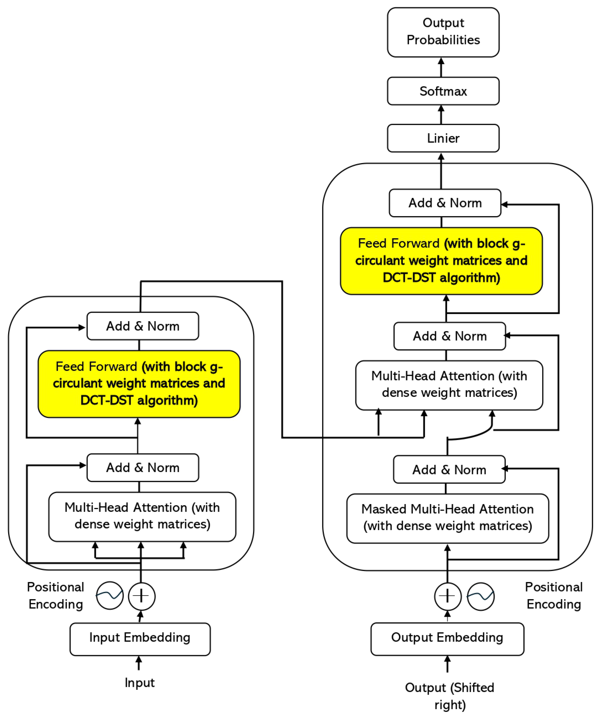
The block g-circulant DCT-DST transformer discussed in this study is a variation of the original transformer model outlined in [2]. This adaptation involves two essential modifications: firstly, the substitution of a block g-circulant matrix for the conventional dense weight matrix, and secondly, the integration of the DCT-DST matrix-vector multiplication algorithm. This integration enables efficient computation when multiplying the block g-circulant matrix with the vector input of each sublayer (Figure 1).

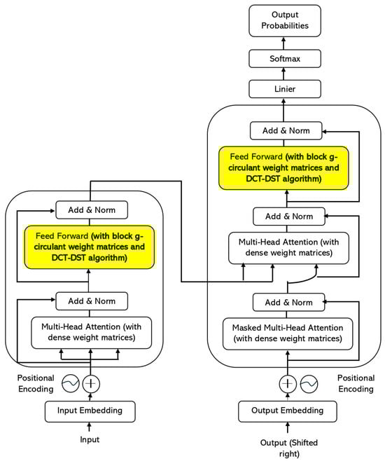
Figure 1. The encoder-decoder structure of the block g-circulant DCT-DST transformer.

3.1. Multihead Attention Sublayer

Two input sequences are applied to the multi-head attention sublayer: a key/value sequence $S_K\in {\mathbb{R}}^{n_K\times d_{model}}$ and a query sequence $S_Q\in {\mathbb{R}}^{n_Q\times d_{model}}$, with $n_K$ and $n_Q$ represent the number of queries and keys/values respectively and $d_{model}$ denote the dimensionality of input and output. Let the number of attention heads be y. By projecting the query sequence and key/value sequence by dense weight matrices, we create queries, keys, and values in ${\mathbb{R}}^{d_k}$, where $dk=d_{model}/y$. For $i=1,\cdots ,y$ and $\alpha =Q,K,V$, we could learn $3y$ separate dense weight matrices $C_{\alpha }^i\in {\mathbb{R}}^{d_k\times d_{model}}$. Rather, for $\alpha =Q,K,V$, we learn a 3-dense weight matrices $C_{\alpha }\in {\mathbb{R}}^{d_{model}\times d_{model}}$ and slice the resulting products y times. It is important that these weight matrices $C_{\alpha }$ have block sizes $c_{attn}$ smaller than $d_k$ to avoid correlations between different attention heads. After obtaining these projections, we calculate the dot product of attention for each attention head:

$$attention(Q^{\left(i\right)},K^{\left(i\right)},V^{\left(i\right)})=softmax\left(\frac{Q^{\left(i\right)}{K}^{\left(i\right)T}}{\sqrt{d_k}}\right)V^{\left(i\right)}$$

(36)

After computing dot-product attention, the output sequences are concatenated into a sequence of shape $(n_k,d_{model})$ and projected through a dense projection matrix $C_{proj}\in {\mathbb{R}}^{d_{model}\times d_{model}}$ with block-size $c_{attn}$. Thus, each dense matrix multihead attention unit learns 4 dense weight matrices $C_Q,C_K,C_V,C_{proj}$ of shape $d_{model}\times d_{model}$ and block-size $c_{attn}<\frac{d_{model}}{y}$.

3.2. Block g-Circulant Positionwise Feedforward Sublayer

The block g-circulant positionwise feedforward sublayer uses two block g-circulant weight matrices. It applies the transformation:

$$a=C_{2}ReLU\left(C_{1}x\right)$$

(37)

where, $C_1\in {\mathbb{R}}^{d_{ff}\times d_{model}}$ has block-size $c_1$ and $C_2\in {\mathbb{R}}^{d_{model}\times d_{ff}}$ has block-size $c_2$, $C_1$ and $C_2$ represent individual g-circulant block matrices, and by default, $d_{ff}=4\times d_{model}$, where $d_{ff}$ denote the dimensionality of the inner-layer. When performing matrix multiplication between $C_1$ and $C_2$ and the multiplier vector, the DCT-DST multiplication algorithm is employed.

3.3. Block Sizes

The block-size parameters $c_{attn},c_1$, and $c_2$ introduce the three-dimensional hyperparameter space. However, we established a single block-size model so that we could test models and iterate quickly. Concerning $c_m$,

$$c_1=c_m;c_2=4\times c_m;c_{attn}=c_m/y$$

(38)

In this case, the maximum value of $c_m$ is $d_{model}$, at which time it is entirely circulant.

3.4. DCT-DST Algorithm

In multiplying block g-circulant weight matrices with any input vector in each transformer layer, we applied the following algorithm, adapted from [28].

• Compute $v=Q_{nmg}{c}_1$ directly, $c_1=C_{nmg}{e}_1$, $e_1={(1,0,0,\cdots ,0)}^T$
• Compute $\widehat{v}={\left(Q_{nmg}{U}_{nmg}\right)}^{T}v$ by DCT and DST
• Form ${\Omega }_{nmg}$
• Compute $y_1=Q_{nmg}x$ directly
• Compute $y_2={\left(Q_{nmg}{U}_{nmg}\right)}^T{y}_1$ by DCT and DST
• Compute $y_3={\Omega }_{nmg}{y}_2$ directly
• Compute $y_4=\left(Q_{nmg}{U}_{nmg}\right)y_3$ by DCT and DST
• Compute $Q_{nmg}^T{y}_4$, i.e., $C_{nmg}x$

4. Experiment and Result

4.1. Data and Experimental Details

This experiment was conducted using data from the TED Talks Open Translation Project’s Portuguese-English datasets, and Tensorflow datasets were then used to load the data. The TED Open Translation Project is a pioneering endeavor by a prominent media platform to subtitle and comprehensively catalog online video content. It represents a groundbreaking initiative in leveraging volunteer translation for public and professional purposes. Among the many talks available within the TED talks transcripts under the Open Translator project, the Portuguese-English transcript is just one of over 2400 talks spanning 109 languages. Portuguese and English are among the top three languages with the highest number of talks in the TED talks collection. It has approximately 52,000 in training examples (Portuguese-English sentence pairs), 1200 in validation examples, and 1800 in test examples.

The dataset was then tokenized using Moses tokenizer as used in the original transformer by [2]. We chose to employ this tokenizer because it is one of the two widely recognized rule-based tokenizers extensively utilized in machine translation and natural language processing experiments. According to [35], the Moses tokenizer has demonstrated superior performance to several other tokenizers, specifically in neural machine translation. We used the code from the TensorFlow.org tutorial on neural machine translation with a transformer and Keras. We utilized the various base model and optimizer setups, which were slightly different from the original transformer model. Distinct from [2], each model applied four layers, not six, as in [2], eight attention heads, and a dropout rate of $0.1$. We set a batch size of 64, while the number of epochs is 20. The feedforward dimensions are four times larger than those of the model. Like [2], we used an Adam optimizer with ${\beta }_1=0.9$; ${\beta }_2=0.98$, and $ϵ={10}^{-9}$. The details of the experiment are provided in Table 1.

Table 1. The experiment details of models training.

Dataset	Portuguese-English translation dataset
	from TED talks Open Translation project
Tokenizer	Moses tokenizer
Training hyperparameters	number of epoch $=20$
	batch size $=64$
	number of layer $=4$
	$d_{model}=16,32,64,128,256$
	$d_{ff}=4\times d_{model}$
	number of head $=8$
	dropout rate $=0.1$
Optimizer	Adam optimizer, ${\beta }_1=0.9$; ${\beta }_2=0.98$, and $ϵ={10}^{-9}$
Weight matrix dimension	$16,32,64,128,256$
g	$0,1,2,3$

The model dimensions have various values depending on the size of the weight matrices being tested. The size of the weight matrices is the combinations of n and m values such that a block g-circulant matrix of dimension 128 was obtained. Choosing a 128-dimensional matrix corresponds to the findings derived from [26]. We also experimented with other matrix dimensions for comparative purposes as part of our analysis. We applied some values of g, inter alia, $g=1$, and other values such that $(nm,g)\ne 1$ and $(nm,g)=1$. $(nm,g)$ denote the greatest common divisor of $nm$ and g.

The model’s name refers to the types of matrices and algorithms employed in the multi-head attention and feed-forward sublayers. We used two types of matrices (Dense and Real Block Circulant Matrices) in conjunction with the DCT-DST algorithm. For instance, the Dense-Block 2-Circulant DCT-DST transformer model means that in the multi-head attention is applied the Dense Matrix and in the feed-forward sublayer is used the real Block 2-Circulant matrix with the DCT-DST algorithm. In this experiment, we trained 3 (three) transformer models with block g-circulant weight matrices and one original transformer model. In each model, experiments were conducted with matrix sizes across five dimensions: 16, 32, 64, 128, and 256 (Table 2).

Table 2. The transformer model being tested along with the g value and size of the weight matrix.

Model	g	${\mathit{d}}_{\mathit{model}}$
Dense-dense (A)	0	$16,32,64,128,256$
Dense-Block 1-Circulant DCT-DST (B)	1	$16,32,64,128,256$
Dense-Block 2-Circulant DCT-DST (C)	2	$16,32,64,128,256$
Dense-Block 3-Circulant DCT-DST (D)	3	$16,32,64,128,256$

4.2. Evaluation

On a held-out set of 500 samples, we evaluated performance using the corpus BLEU (Bilingual Evaluation Understudy) score. This figure corresponds to [36]. Statistically, a sample size of 500 can be classified as significant, making it sufficiently robust for conclusion.

BLEU serves as a metric designed to evaluate machine-translated text automatically. It quantifies the similarity between the machine-translated text and a set of high-quality reference translations, generating a score ranging from zero to one. BLEU’s notable strength is its strong correlation with human judgments. It achieves this by averaging individual sentence judgment errors across a test corpus rather than attempting to precisely determine human judgment for every single sentence [36,37]. In our study, the corpus BLEU score employed the English sentence as its single reference and the top English sentence output of beam search as the hypothesis for each pair of Portuguese and English sentences in the evaluation set. Aggregating references and hypotheses across all pairings produced the corpus BLEU.

4.3. Result and Discussion

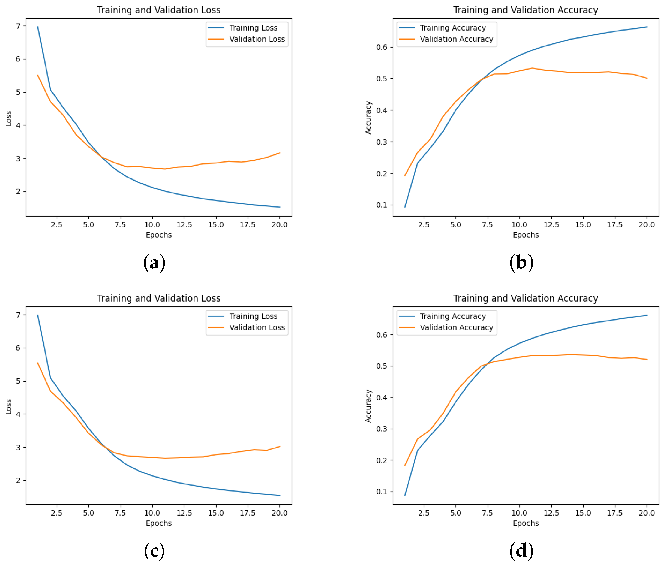
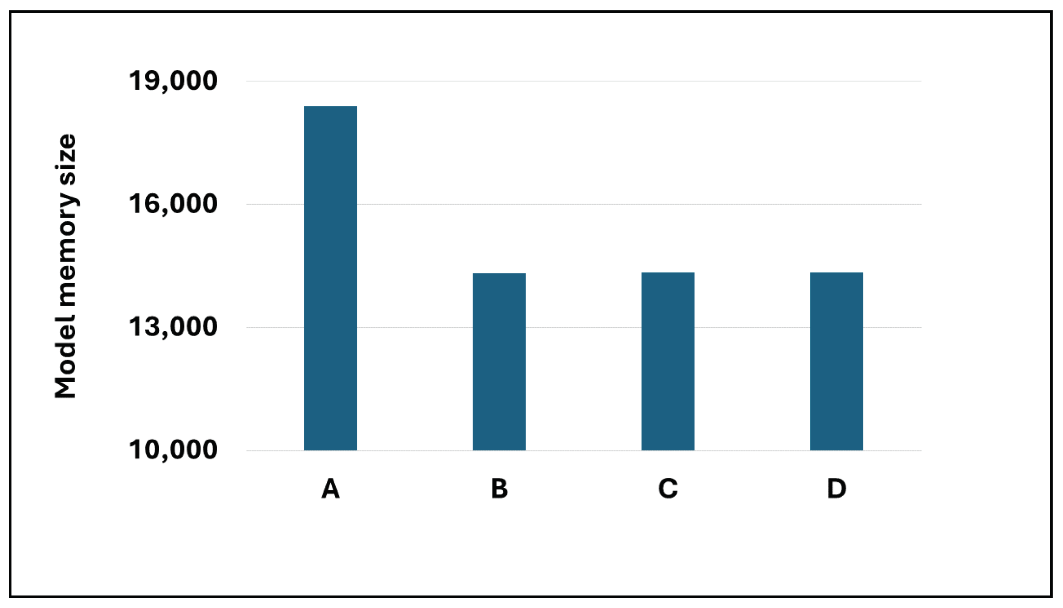
Based on the analysis of multiple model samples displayed in Figure 2, it’s evident that the overall models avoid overfitting, demonstrating their capability for predictive tasks. Reviewing the experimental outcomes outlined in Table 3, the Dense-Block 1-circulant DCT-DST model notably surpasses the Dense-Dense model in BLEU score and model memory efficiency. Specifically, it achieves a $4.1\%$ higher BLEU score and demonstrates a $22.14\%$ improvement in model memory utilization. However, across other metrics, the performance of the block g-circulant matrix-based model needs to catch up to the Dense-Dense model. During testing on the test dataset, the Dense-Dense model excels notably in test duration. Furthermore, across similar matrix dimensions, all models achieve loss values that exhibit marginal differences. Notably, the block g-circulant model group with $(nm,g)=1$ tends to outperform the group where $(nm,g)\ne 1$, both in terms of loss and accuracy metrics. Figure 3, Figure 4, Figure 5 and Figure 6 provides a holistic view of the comparison among diverse g values, highlighting the fluctuations in loss, accuracy, BLEU score, and model memory size.

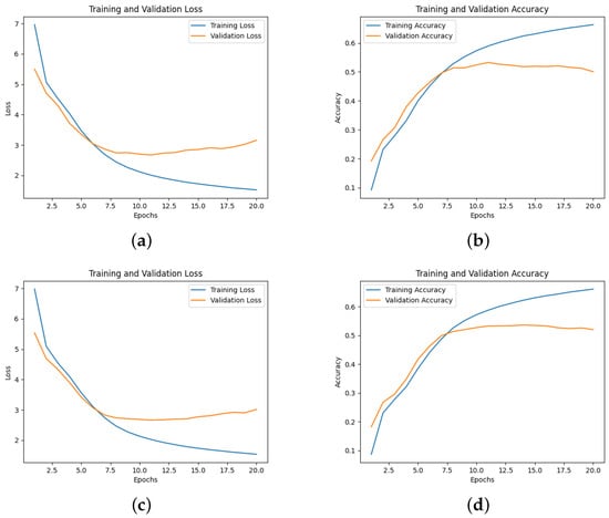
Figure 2. (a) The loss of Dense-Block 2-Circulant DCT-DST model; (b) The accuracy of Dense-Block 2-Circulant DCT-DST model; (c) The loss of Dense-Block 3-Circulant DCT-DST model; (d) The Accuracy of Dense-Block 3-Circulant DCT-DST model.

Table 3. The evaluated metrics across the four transformer models include accuracy, loss, test duration, BLEU score, and model memory consumption.

Model	g	${\mathit{d}}_{\mathit{model}}$	Loss	Accuracy (%)	Test Duration (Second)	BLEU (%)	Model Memory (KB)
		16	$4.027$	$0.327$	$7.831$	$2.78$	1751
		32	$2.963$	$0.485$	$7.907$	$2.71$	3546
A	0	64	$2.404$	$0.569$	$8.260$	$2.71$	7540
		128	$2.320$	$0.607$	$8.895$	$25.43$	$\mathrm{18,394}$
		256	$2.219$	$0.616$	$9.348$	$25.43$	$\mathrm{50,855}$
		16	$4.1058$	$0.3186$	$8.9704$	$1.75$	1714
		32	$3.3718$	$0.4201$	$9.5401$	$11.64$	3227
B	1	64	$2.651$	$0.5244$	$11.566$	$22.23$	6542
		128	$2.373$	$0.579$	$27.839$	$26.47$	$\mathrm{14,322}$
		256	$2.3089$	$0.5855$	$121.908$	$24.65$	$\mathrm{34,491}$
		16	$4.151$	$0.317$	$17.591$	$2.29$	1732
		32	$3.338$	$0.425$	$24.934$	$9.06$	3246
C	2	64	$2.619$	$0.528$	$31.145$	$20.8$	6560
		128	$2.448$	$0.555$	$59.918$	$21.69$	$\mathrm{14,340}$
		256	$2.323$	$0.577$	$180.119$	$24.18$	$\mathrm{34,509}$
		16	$4.0974$	$0.3232$	$18.4132$	$2.54$	1732
		32	$3.2157$	$0.4404$	$24.5743$	$11.64$	3246
D	3	64	$2.6102$	$0.5312$	$36.9716$	$21.35$	6560
		128	$2.373$	$0.570$	$68.211$	$24.12$	$\mathrm{14,340}$
		256	$2.3079$	$0.5798$	$283.2846$	$24.98$	$\mathrm{34,509}$

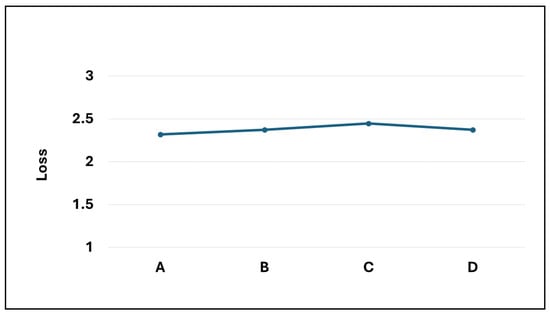
Figure 3. The loss values for the four transformer models.

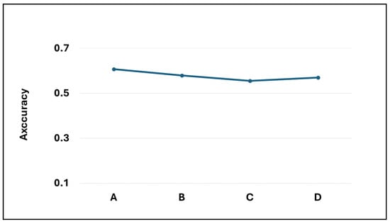
Figure 4. The accuracy values for the four transformer models.

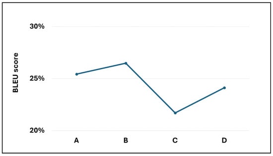
Figure 5. The BLEU score for the four transformer models.

Figure 6. The Model memory size for the four transformer models.

In general, the transformer model employing the block g-circulant weight matrix boasts a more efficient model memory size than the Dense-Dense model. This enhanced efficiency can be credited to utilizing the block g-circulant matrix, a structured matrix falling within the category of low displacement rank (LDR) matrices [12]. This discovery corroborates earlier research detailed in [26,28,29], which similarly highlighted the benefits of both block circulant matrices and circulant matrices through experimental evidence—the block g-circulant matrices allowing us to leverage the concept of data-sparsity. Data sparsity implies that representing an $n\times n$ matrix necessitates fewer than $O\left(n^2\right)$ parameters. Unlike traditional sparse matrices, data-sparse matrices aren’t mandated to contain zero entries; instead, a relationship exists among the matrix entries. Moreover, efficient algorithms, such as computing the matrix-vector product with any vector, can be achieved with fewer than $O\left(n^2\right)$ operations [12]. This approach is expected to reduce the number of model training parameters utilized in the experiment, consequently diminishing the demand for storage space. Moreover, the reduced storage space requirement is believed to stem from implementing the DCT-DST algorithm, elaborated upon in [28].

Additionally, the relatively prolonged test duration observed in the block g-circulant model experiments likely arises from employing a vector matrix multiplication algorithm involving more intricate procedural steps, such as the algorithm DCT-DST. Initially, some people anticipated that implementing the algorithm would streamline the testing process, but contrary to expectations, the opposite happened. This can be attributed to the algorithm’s relatively intricate structure and the deep transformer architecture, which involves a significant number of weight matrix and input vector multiplication operations.

5. Conclusions

Incorporating a structured block g-circulant matrix as a weight matrix, combined with the DCT-DST algorithm for multiplication with the input vector in the transformer model, effectively elevated the BLEU score and conserved storage space. However, this approach resulted in a slight reduction in accuracy and an extension of testing time. In a mathematical context, the Kronecker product operation plays a pivotal role in defining the matrices used in the algorithm, enabling the execution of the DCT-DST algorithm on the multiplication of the weight matrix with the transformer input vector.

References

- Mitsuda, K.; Higashinaka, R.; Sugiyama, H.; Mizukami, M.; Kinebuchi, T.; Nakamura, R.; Adachi, N.; Kawabata, H. Fine-Tuning a Pre-trained Transformer-Based Encoder-Decoder Model with User-Generated Question-Answer Pairs to Realize Character-like Chatbots. In Conversational AI for Natural Human-Centric Interaction: Proceedings of the 12th International Workshop on Spoken Dialogue System Technology, Singapore, IWSDS 2021; Springer Nature: Singapore, 2022; pp. 277–290. [Google Scholar]
- Vaswani, A.; Shazeer, N.; Parmar, N.; Uszkoreit, J.; Jones, L.; Gomez, A.N.; Kaiser, L.; dan Polosukhin, I. Attention is all you need. arXiv 2017, arXiv:1706.03762. [Google Scholar]
- Ranganathan, J.; Abuka, G. Text summarization using transformer model. In Proceedings of the 2022 Ninth International Conference on Social Networks Analysis, Management and Security (SNAMS), Milan, Italy, 29 November–1 December 2022; pp. 1–5. [Google Scholar]
- Arnab, A.; Dehghani, M.; Heigold, G.; Sun, C.; Lucic, M.; Schmid, C. Vivit: A video vision transformer. In Proceedings of the IEEE/CVF International Conference on Computer Vision, Montreal, QC, Canada, 10–17 October 2021; pp. 6836–6846. [Google Scholar]
- Zeng, P.; Zhang, H.; Song, J.; Gao, L. S2 transformer for image captioning. In Proceedings of the International Joint Conferences on Artificial Intelligence, Vienna, Austria, 23–29 July 2022; pp. 1608–1614. [Google Scholar]
- Bazi, Y.; Bashmal, L.; Rahhal, M.M.A.; Dayil, R.A.; Ajlan, N.A. Vision transformers for remote sensing image classification. Remote Sens. 2021, 13, 516. [Google Scholar] [CrossRef]
- Toral, A.; Oliver, A.; Ballestín, P.R. Machine translation of novels in the age of transformer. arXiv 2020, arXiv:2011.14979. [Google Scholar]
- Araabi, A.; Monz, C. Optimizing transformer for low-resource neural machine translation. arXiv 2020, arXiv:2011.02266. [Google Scholar]
- Tian, T.; Song, C.; Ting, J.; Huang, H. A French-to-English machine translation model using transformer network. Procedia Comput. Sci. 2022, 199, 1438–1443. [Google Scholar] [CrossRef]
- Ahmed, K.; Keskar, N.S.; Socher, R. Weighted transformer network for machine translation. arXiv 2017, arXiv:1711.02132. [Google Scholar]
- Wang, Q.; Li, B.; Xiao, T.; Zhu, J.; Li, C.; Wong, D.F.; Chao, L.S. Learning deep transformer models for machine translation. arXiv 2019, arXiv:1906.01787. [Google Scholar]
- Kissel, M.; Diepold, K. Structured Matrices and Their Application in Neural Networks: A Survey. New Gener. Comput. 2023, 41, 697–722. [Google Scholar] [CrossRef]
- Keles, F.D.; Wijewardena, P.M.; Hegde, C. On the computational complexity of self-attention. In Proceedings of the 34th International Conference on Algorithmic Learning Theory, Singapore, 20–23 February 2022; PMLR:2023. pp. 597–619. [Google Scholar]
- Pan, Z.; Chen, P.; He, H.; Liu, J.; Cai, J.; Zhuang, B. Mesa: A memory-saving training framework for transformers. arXiv 2021, arXiv:2111.11124. [Google Scholar]
- Yang, H.; Zhao, M.; Yuan, L.; Yu, Y.; Li, Z.; Gu, M. Memory-efficient Transformer-based network model for Traveling Salesman Problem. Neural Netw. 2023, 161, 589–597. [Google Scholar] [CrossRef]
- Sohoni, N.S.; Aberger, C.R.; Leszczynski, M.; Zhang, J.; Ré, C. Low-memory neural network training: A technical report. arXiv 2019, arXiv:1904.10631. [Google Scholar]
- Sainath, T.N.; Kingsbury, B.; Sindhwani, V.; Arisoy, E.; Ramabhadran, B. Low-rank matrix factorization for deep neural network training with high-dimensional output targets. In Proceedings of the IEEE International Conference on Acoustics, Speech and Signal Processing, Vancouver, BC, Canada, 26–31 May 2013; pp. 6655–6659. [Google Scholar]
- Sindhwani, V.; Sainath, T.; Kumar, S. Structured transforms for small-footprint deep learning. arXiv 2015, arXiv:1510.01722. [Google Scholar]
- Cheng, Y.; Yu, F.X.; Feris, R.S.; Kumar, S.; Choudhary, A.; Chang, S. An exploration of parameter redundancy in deep networks with circulant projections. In Proceedings of the IEEE International Conference on Computer Vision, Santiago, Chile, 11–18 December 2015; pp. 2857–2865. [Google Scholar]
- Ding, C.; Liao, S.; Wang, Y.; Li, Z.; Liu, N.; Zhuo, Y.; Wang, C.; Qian, X.; Bai, Y.; Yuan, G.; et al. Circnn: Accelerating and compressing deep neural networks using block-circulant weight matrices. In Proceedings of the 50th Annual IEEE/ACM International Symposium on Microarchitecture, Boston, MA, USA, 14–17 October 2017; pp. 395–408. [Google Scholar]
- Yang, Z.; Moczulski, M.; Denil, M.; Freitas, N.D.; Song, L.; Wang, Z. Deep fried convnets. In Proceedings of the IEEE International Conference on Computer Vision, Santiago, Chile, 7–13 December 2015. [Google Scholar]
- Thomas, A.; Gu, A.; Dao, T.; Rudra, A.; Ré, C. Learning compressed transforms with low displacement rank. arXiv 2018, arXiv:1810.02309. [Google Scholar]
- Dao, T.; Gu, A.; Eichhorn, M.; Rudra, A.; Ré, C. Learning fast algorithms for linear transforms using butterfly factorizations. Proc. Mach. Learn. Res. 2019, 97, 1517–1527. [Google Scholar] [PubMed]
- Pan, V. Structured Matrices and Polynomials: Unified Superfast Algorithms; Springer Science and Business Media: Boston, MA, USA; New York, NY, USA, 2001. [Google Scholar]
- Davis, P.J. Circulant Matrices; Wiley: New York, NY, USA, 1979; Volume 2. [Google Scholar]
- Asriani, E.; Muchtadi-Alamsyah, I.; Purwarianti, A. Real Block-Circulant Matrices and DCT-DST Algorithm for Transformer Neural Network. Front. Appl. Math. Stat. 2023, 9, 1260187. [Google Scholar] [CrossRef]
- Asriani, E.; Muchtadi-Alamsyah, I.; Purwarianti, A. g-Circulant Matrices and Its Matrix-Vector Multiplication Algorithm for Transformer Neural Networks. AIP Conf. 2024. post-acceptance. [Google Scholar]
- Liu, Z.; Chen, S.; Xu, W.; Zhang, Y. The eigen-structures of real (skew) circulant matrices with some applications. Comput. Appl. Math. 2019, 38, 1–13. [Google Scholar] [CrossRef]
- Reid, S.; dan Mistele, M. Fast Fourier Transformed Transformers: Circulant Weight Matrices for NMT Compression. 2019. Available online: https://web.stanford.edu/class/archive/cs/cs224n/cs224n.1194/reports/custom/15722831.pdf (accessed on 23 May 2024).
- Saxena, A.; Fernandes, F.C. DCT/DST-based transform coding for intra prediction in image/video coding. IEEE Trans. Image Process. 2013, 22, 3974–3981. [Google Scholar] [CrossRef]
- Park, W.; Lee, B.; Kim, M. Fast computation of integer DCT-V, DCT-VIII, and DST-VII for video coding. IEEE Trans. Image Process. 2019, 28, 5839–5851. [Google Scholar] [CrossRef]
- Olson, B.; Shaw, S.; Shi, C.; Pierre, C.; Parker, R. Circulant matrices and their application to vibration analysis. Appl. Mech. Rev. 2014, 66, 040803. [Google Scholar] [CrossRef]
- Serra-Capizzano, S.; Debora, S. A note on the eigenvalues of g-circulants (and of g-Toeplitz, g-Hankel matrices). Calcolo 2014, 51, 639–659. [Google Scholar] [CrossRef]
- Wilkinson, J.H. The Algebraic Eigenvalue Problem; Clarendon: Oxford, UK, 1965; Volume 662. [Google Scholar]
- Domingo, M.; Garcıa-Martınez, M.; Helle, A.; Casacuberta, F.; Herranz, M. How much does tokenization affect neural machine translation? arXiv 2018, arXiv:1812.08621. [Google Scholar]
- Papineni, K.; Roukos, S.; Ward, T.; Zhu, W.J. Bleu: A method for automatic evaluation of machine translation. In Proceedings of the 40th Annual Meeting of the Association for Computational Linguistics, Philadelphia, PA, USA, 6–12 July 2002; pp. 311–318. [Google Scholar]
- Post, M. A call for clarity in reporting BLEU scores. arXiv 2018, arXiv:1804.08771. [Google Scholar]
Disclaimer/Publisher’s Note: The statements, opinions and data contained in all publications are solely those of the individual author(s) and contributor(s) and not of MDPI and/or the editor(s). MDPI and/or the editor(s) disclaim responsibility for any injury to people or property resulting from any ideas, methods, instructions or products referred to in the content. |
© 2024 by the authors. Licensee MDPI, Basel, Switzerland. This article is an open access article distributed under the terms and conditions of the Creative Commons Attribution (CC BY) license (https://creativecommons.org/licenses/by/4.0/).