
Intelligent Fault Diagnosis Across Varying Working Conditions Using Triplex Transfer LSTM for Enhanced Generalization


Abstract
:1. Introduction
- (1)
- Deep learning models generally necessitate a substantial amount of labeled data to generalize effectively. The primary problem with fault diagnosis is the challenge of gathering sufficient data on various fault conditions, as machines rarely exhibit faults during normal operation. The scarcity of data makes it difficult to train models effectively, potentially leading to overfitting (a phenomenon where models perform well on training data but underperform on new, unseen data) [32].
- (2)
- The expense associated with expert labeling of the acquired data poses a significant financial and resource burden. Because it may be impossible to detect every possible fault scenario, especially in industrial complex machinery, accurate fault class labeling based on the machine’s operating conditions typically requires skilled personnel [33].
- (3)
- Variations in loads, speeds, and temperatures are common operating conditions for machines in industrial settings. Domain shift, in which data distribution changes between two domains, is the result of this unpredictability and variability. Due to this shift, DL models trained on data from one domain may struggle to generalize effectively under new conditions, which makes them unreliable for defect diagnosis in the real-world scenarios [34].
1.1. Research Gap
- The requirement of uniform data distribution for training and testing datasets should be addressed. However, in practical situations, variations in machine operating conditions may modify vibrational patterns, thereby affecting the data obtained from the actual operational platform. Additionally, training and testing datasets have unequal data samples and distributions.
- Currently, models are typically trained independently for each task, limiting their applicability to new working conditions (e.g., varying loads and speeds) and highlighting the need for significant improvements in fault identification accuracy.
- Acquiring data labels in the context of big data can be tedious because of the inherent limitations, including labor-intensive and time-consuming procedures.
- When working with sparse labeled data, TL performs fault diagnosis more efficiently. Overfitting is a significant problem when using pre-trained models, especially with small datasets, due to the advanced nature of these models and their typically numerous parameters.
1.2. Key Contributions
- This paper proposes a Triplex Transfer Long Short-Term Memory (TTLSTM) method, which uses a deep LSTM network to learn long-term dependencies and intricate non-linear correlations in the data.
- This method uses the empirical mode decomposition (EMD) technique to extract features from non-stationary and non-linear vibrational signals, as well as the Pearson correlation coefficient (PCC) feature selection method, which improves the model’s diagnostic performance.
- With small, labeled target domain data, a fine-tuning strategy-based TL method is designed for effective fault diagnosis. The proposed method overcomes the limitations of insufficient labeled data and domain shift problems by leveraging transfer learning and fine-tuning strategies to improve the model’s adaptability across diverse working conditions (from low motor speed to high motor speed and vice versa).
- To alleviate the overfitting problem, L2 regularization TL is utilized, particularly in scenarios with limited labeled target data. The ablation experiments are also conducted to validate the positive impact of L2 regularization in the TTLSTM model. The developed model is then compared with state-of-the-art fault diagnosis methods to ensure its robust performance across WCs and its ability to generalize well to new unknown data.
2. Problem Description and Preliminary
2.1. Concept of Transfer Learning
2.2. Long Short-Term Memory Network
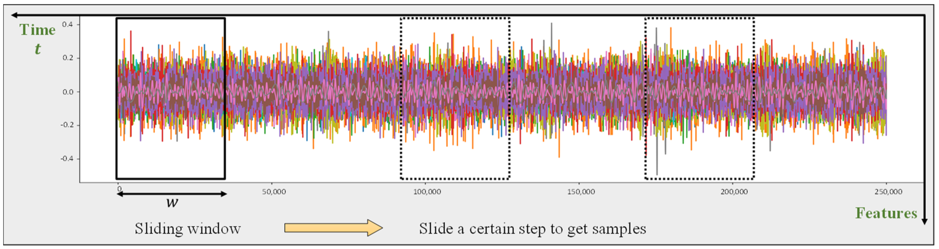
2.3. Sliding Window
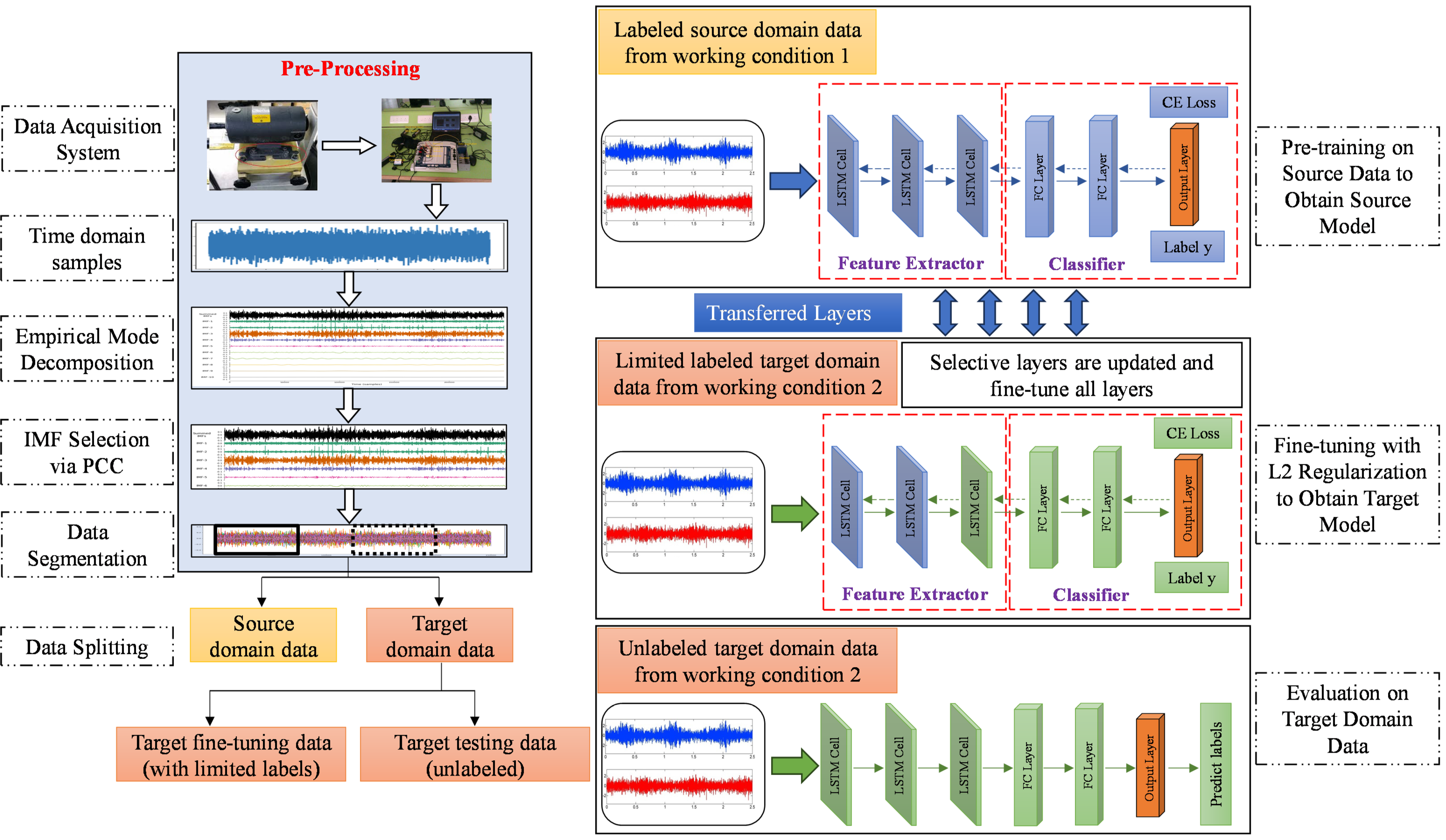
3. Proposed Methodology
3.1. Pre-Processing Overview
3.1.1. Normalization
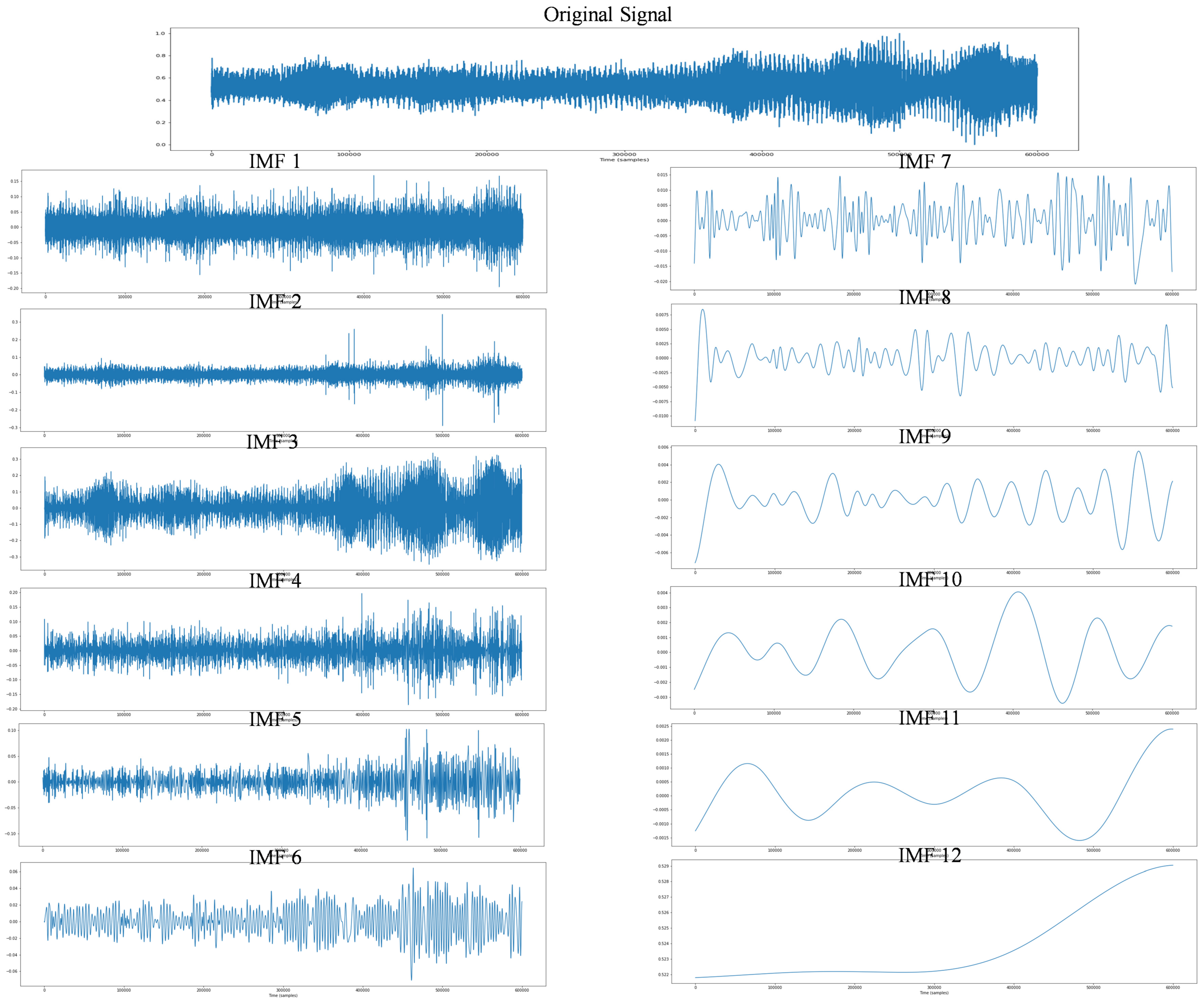
3.1.2. Empirical Mode Decomposition
- To create the upper and lower envelopes, locate all the local extrema, and then use a cubic spline to connect the local maxima and minima. There should be no information lost between the envelopes.
- The first component is the difference between the mean of the upper and lower envelope () and the signal x(t).To create IMFs, the following conditions should be fulfilled:
- A maximum of one (1) difference is allowed between the number of extrema and zero crossings.
- The midpoint between the upper and lower bounds is always zero.
- If these above conditions are fulfilled, then will be the first IMF. If this condition is not satisfied, will become the original signal, and again, other IMF will be generated . This process repeats n-times, as indicated byThis logic can be regarded as .
- Differentiate from
3.1.3. Feature Selection via Pearson Correlation Coefficient
3.2. The Architecture of TTLSTM Model
3.2.1. Pre-Training Network
3.2.2. Fine-Tuning Network
3.2.3. Optimizer and Activation Function
3.2.4. Classification Loss and Classifier
3.2.5. L2 Regularization Transfer Learning
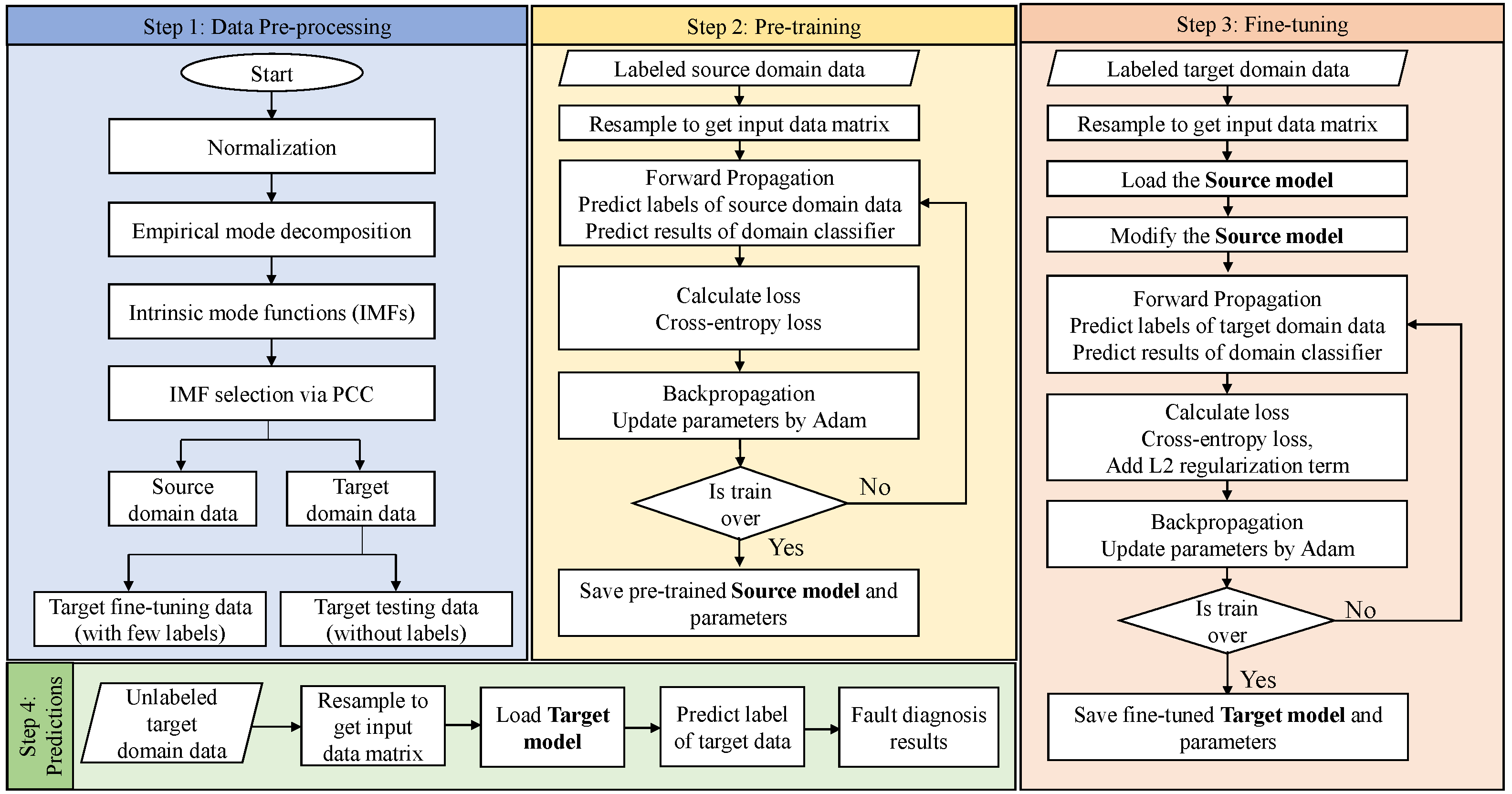
3.3. Overview of Proposed Methodology
4. Experimental Study
4.1. Dataset Description
- To induce the unbalance fault into the ABVT, 20 g screws are inserted in a center-hug configuration on the inertia disc.
- To create the horizontal misalignment fault, move the DC motor’s base in the horizontal plane and measure with a digital caliper. The horizontal misalignments are limited to no more than 0.5 mm.
- Placing shims of defined thickness on the electric motor’s base causes a vertical misalignment. A vertical deviation of 0.51 mm is considered.
4.2. Detailed Pre-Processing Step
4.3. Diagnostic Performance of the Proposed Method
4.3.1. Experimental Design
4.3.2. Source Domain-Based Effectiveness Evaluation (Pre-Training)
4.3.3. Evaluating Transferability Under Varying WCs of (L → H)
4.3.4. Special Case: Evaluating Transferability Under Varying WCs of (H → L)
4.3.5. Analysis
4.3.6. Ablation Study: Effect of L2 Regularization on the TTLSTM Model
4.4. Comparative Analysis
4.4.1. Transfer Learning vs. Without Transfer Learning Across Varying Working Conditions
4.4.2. Comparison with Other Methods
4.5. Practical Implications in Industrial Operations
5. Conclusions
Author Contributions
Funding
Data Availability Statement
Acknowledgments
Conflicts of Interest
Nomenclature
| ACA | Average Classification Accuracy |
| AE | Auto Encoder |
| ANN | Artificial Neural Network |
| BDA | Balanced Distribution Adaptation |
| CNN | Convolutional Neural Networks |
| DBN | Deep Belief Network |
| DL | Deep Learning |
| EMD | Empirical Mode Decomposition |
| FFT | Fast Fourier Transform |
| GNN | Graph Neural Networks |
| IMFs | Intrinsic Mode Decompositions |
| JDA | Joint Distribution Adaptation |
| KNN | K-nearest Neighbor |
| LSTM | Long Short-Term Memory |
| OCA | Overall Classification Accuracy |
| PCA | Principal Component Analysis |
| PCC | Pearson Correlation Coefficients |
| RF | Random Forest |
| RNN | Recurrent Neural Networks |
| SVM | Support Vector Machine |
| TCA | Transfer Component Analysis |
| TL | Transfer Learning |
| WCs | Working Conditions |
| WT | Wavelet Transform |
| XGBoost | Extreme Gradient Boosting |
References
- Sun, C.; Ma, M.; Zhao, Z.; Chen, X. Sparse deep stacking network for fault diagnosis of motor. IEEE Trans. Ind. Inform. 2018, 14, 3261–3270. [Google Scholar] [CrossRef]
- Shao, H.; Jiang, H.; Zhang, H.; Liang, T. Electric locomotive bearing fault diagnosis using a novel convolutional deep belief network. IEEE Trans. Ind. Electron. 2017, 65, 2727–2736. [Google Scholar] [CrossRef]
- Chen, J.; Pan, J.; Li, Z.; Zi, Y.; Chen, X. Generator bearing fault diagnosis for wind turbine via empirical wavelet transform using measured vibration signals. Renew. Energy 2016, 89, 80–92. [Google Scholar] [CrossRef]
- Xi, W.; Li, Z.; Tian, Z.; Duan, Z. A feature extraction and visualization method for fault detection of marine diesel engines. Measurement 2018, 116, 429–437. [Google Scholar] [CrossRef]
- Sharma, V.; Parey, A. A review of gear fault diagnosis using various condition indicators. Procedia Eng. 2016, 144, 253–263. [Google Scholar] [CrossRef]
- Li, W.; Huang, R.; Li, J.; Liao, Y.; Chen, Z.; He, G.; Yan, R.; Gryllias, K. A perspective survey on deep transfer learning for fault diagnosis in industrial scenarios: Theories, applications and challenges. Mech. Syst. Signal Process. 2022, 167, 108487. [Google Scholar] [CrossRef]
- Li, C.; Zhang, S.; Qin, Y.; Estupinan, E. A systematic review of deep transfer learning for machinery fault diagnosis. Neurocomputing 2020, 407, 121–135. [Google Scholar] [CrossRef]
- Shao, H.; Jiang, H.; Wang, F.; Wang, Y. Rolling bearing fault diagnosis using adaptive deep belief network with dual-tree complex wavelet packet. ISA Trans. 2017, 69, 187–201. [Google Scholar] [CrossRef]
- Yuan, H.; Wang, X.; Sun, X.; Ju, Z. Compressive sensing-based feature extraction for bearing fault diagnosis using a heuristic neural network. Meas. Sci. Technol. 2017, 28, 065018. [Google Scholar] [CrossRef]
- Neupane, D.; Seok, J. Bearing fault detection and diagnosis using case western reserve university dataset with deep learning approaches: A review. IEEE Access 2020, 8, 93155–93178. [Google Scholar] [CrossRef]
- Boudiaf, A.; Moussaoui, A.; Dahane, A.; Atoui, I. A comparative study of various methods of bearing faults diagnosis using the case Western Reserve University data. J. Fail. Anal. Prev. 2016, 16, 271–284. [Google Scholar] [CrossRef]
- Bangalore, P.; Tjernberg, L.B. An artificial neural network approach for early fault detection of gearbox bearings. IEEE Trans. Smart Grid 2015, 6, 980–987. [Google Scholar] [CrossRef]
- Abid, F.B.; Zgarni, S.; Braham, A. Distinct bearing faults detection in induction motor by a hybrid optimized SWPT and aiNet-DAG SVM. IEEE Trans. Energy Convers. 2018, 33, 1692–1699. [Google Scholar] [CrossRef]
- Wang, D. K-nearest neighbors based methods for identification of different gear crack levels under different motor speeds and loads: Revisited. Mech. Syst. Signal Process. 2016, 70, 201–208. [Google Scholar] [CrossRef]
- Roy, S.S.; Dey, S.; Chatterjee, S. Autocorrelation aided random forest classifier-based bearing fault detection framework. IEEE Sens. J. 2020, 20, 10792–10800. [Google Scholar] [CrossRef]
- Behseresht, S.; Love, A.; Valdez Pastrana, O.A.; Park, Y.H. Enhancing Fused Deposition Modeling Precision with Serial Communication-Driven Closed-Loop Control and Image Analysis for Fault Diagnosis-Correction. Materials 2024, 17, 1459. [Google Scholar] [CrossRef]
- Sulaiman, M.; Khan, N.A.; Alshammari, F.S.; Laouini, G. Performance of heat transfer in micropolar fluid with isothermal and isoflux boundary conditions using supervised neural networks. Mathematics 2023, 11, 1173. [Google Scholar] [CrossRef]
- Khan, N.A.; Hussain, S.; Spratford, W.; Goecke, R.; Kotecha, K.; Jamwal, P. Deep Learning-Driven Analysis of a Six-Bar Mechanism for Personalized Gait Rehabilitation. J. Comput. Inf. Sci. Eng. 2024, 15, 011001. [Google Scholar] [CrossRef]
- Banitaba, F.S.; Aygun, S.; Najafi, M.H. Late Breaking Results: Fortifying Neural Networks: Safeguarding Against Adversarial Attacks with Stochastic Computing. arXiv 2024, arXiv:2407.04861. [Google Scholar]
- Shao, H.; Jiang, H.; Li, X.; Wu, S. Intelligent fault diagnosis of rolling bearing using deep wavelet auto-encoder with extreme learning machine. Knowl. -Based Syst. 2018, 140, 1–14. [Google Scholar]
- Xie, J.; Du, G.; Shen, C.; Chen, N.; Chen, L.; Zhu, Z. An end-to-end model based on improved adaptive deep belief network and its application to bearing fault diagnosis. IEEE Access 2018, 6, 63584–63596. [Google Scholar] [CrossRef]
- Jiang, H.; Li, X.; Shao, H.; Zhao, K. Intelligent fault diagnosis of rolling bearings using an improved deep recurrent neural network. Meas. Sci. Technol. 2018, 29, 065107. [Google Scholar] [CrossRef]
- Pan, J.; Zi, Y.; Chen, J.; Zhou, Z.; Wang, B. LiftingNet: A novel deep learning network with layerwise feature learning from noisy mechanical data for fault classification. IEEE Trans. Ind. Electron. 2017, 65, 4973–4982. [Google Scholar] [CrossRef]
- Wu, J. Introduction to Convolutional Neural Networks; National Key Lab for Novel Software Technology, Nanjing University: Nanjing, China, 2017; Volume 5, pp. 1–31. [Google Scholar]
- Liu, H.; Zhou, J.; Zheng, Y.; Jiang, W.; Zhang, Y. Fault diagnosis of rolling bearings with recurrent neural network-based autoencoders. ISA Trans. 2018, 77, 167–178. [Google Scholar] [CrossRef] [PubMed]
- Qiao, M.; Yan, S.; Tang, X.; Xu, C. Deep convolutional and LSTM recurrent neural networks for rolling bearing fault diagnosis under strong noises and variable loads. IEEE Access 2020, 8, 66257–66269. [Google Scholar] [CrossRef]
- Zhang, Z.; Wu, L. Graph neural network-based bearing fault diagnosis using Granger causality test. Expert Syst. Appl. 2024, 242, 122827. [Google Scholar] [CrossRef]
- Cui, M.; Wang, Y.; Lin, X.; Zhong, M. Fault diagnosis of rolling bearings based on an improved stack autoencoder and support vector machine. IEEE Sens. J. 2020, 21, 4927–4937. [Google Scholar] [CrossRef]
- Niu, G.; Wang, X.; Golda, M.; Mastro, S.; Zhang, B. An optimized adaptive PReLU-DBN for rolling element bearing fault diagnosis. Neurocomputing 2021, 445, 26–34. [Google Scholar] [CrossRef]
- Chia, Z.C.; Lim, K.H.; Tan, T.P.L. Two-phase Switching Optimization Strategy in LSTM Model for Predictive Maintenance. In Proceedings of the 2021 International Conference on Green Energy, Computing and Sustainable Technology (GECOST), Miri, Malaysia, 7–9 July 2021; pp. 1–6. [Google Scholar]
- Ma, M.; Mao, Z. Deep-convolution-based LSTM network for remaining useful life prediction. IEEE Trans. Ind. Inform. 2020, 17, 1658–1667. [Google Scholar] [CrossRef]
- Alzubaidi, L.; Zhang, J.; Humaidi, A.J.; Al-Dujaili, A.; Duan, Y.; Al-Shamma, O.; Santamaría, J.; Fadhel, M.A.; Al-Amidie, M.; Farhan, L. Review of deep learning: Concepts, CNN architectures, challenges, applications, future directions. J. Big Data 2021, 8, 53. [Google Scholar] [CrossRef]
- Farahani, A.; Voghoei, S.; Rasheed, K.; Arabnia, H.R. A brief review of domain adaptation. In Advances in Data Science and Information Engineering, Proceedings of the ICDATA 2020, Las Vegas, NV, USA, 27–30 July 2020 and IKE 2020, Las Vegas, NV, USA, 27–30 July 2020; Springer: Cham, Switzerland, 2021; pp. 877–894. [Google Scholar]
- Misbah, I.; Lee, C.; Keung, K. Fault diagnosis in rotating machines based on transfer learning: Literature review. Knowl. -Based Syst. 2023, 283, 111158. [Google Scholar] [CrossRef]
- Pan, S.J.; Yang, Q. A survey on transfer learning. IEEE Trans. Knowl. Data Eng. 2009, 22, 1345–1359. [Google Scholar] [CrossRef]
- Han, T.; Liu, C.; Wu, R.; Jiang, D. Deep transfer learning with limited data for machinery fault diagnosis. Appl. Soft Comput. 2021, 103, 107150. [Google Scholar] [CrossRef]
- Shao, S.; McAleer, S.; Yan, R.; Baldi, P. Highly accurate machine fault diagnosis using deep transfer learning. IEEE Trans. Ind. Inform. 2018, 15, 2446–2455. [Google Scholar] [CrossRef]
- Su, J.; Wang, H. Fine-tuning and efficient VGG16 transfer learning fault diagnosis method for rolling bearing. In Proceedings of the IncoME-VI and TEPEN 2021: Performance Engineering and Maintenance Engineering, Tianjin, China, 20–23 October 2021; Springer: Cham, Swizerland, 2022; pp. 453–461. [Google Scholar]
- Sun, Q.; Zhang, Y.; Chu, L.; Tang, Y.; Xu, L.; Li, Q. Fault Diagnosis of Gearbox Based on Cross-domain Transfer Learning with Fine-tuning Mechanism Using Unbalanced Samples. IEEE Trans. Instrum. Meas. 2024, 73, 1–10. [Google Scholar] [CrossRef]
- Zhong, H.; Yu, S.; Trinh, H.; Lv, Y.; Yuan, R.; Wang, Y. Fine-tuning transfer learning based on DCGAN integrated with self-attention and spectral normalization for bearing fault diagnosis. Measurement 2023, 210, 112421. [Google Scholar] [CrossRef]
- Liu, Q.; Huang, C. A fault diagnosis method based on transfer convolutional neural networks. IEEE Access 2019, 7, 171423–171430. [Google Scholar] [CrossRef]
- Tang, T.; Wu, J.; Chen, M. Lightweight model-based two-step fine-tuning for fault diagnosis with limited data. Meas. Sci. Technol. 2022, 33, 125112. [Google Scholar] [CrossRef]
- Shao, H.; Li, W.; Xia, M.; Zhang, Y.; Shen, C.; Williams, D.; Kennedy, A.; de Silva, C.W. Fault diagnosis of a rotor-bearing system under variable rotating speeds using two-stage parameter transfer and infrared thermal images. IEEE Trans. Instrum. Meas. 2021, 70, 1–11. [Google Scholar] [CrossRef]
- Han, T.; Zhou, T.; Xiang, Y.; Jiang, D. Cross-machine intelligent fault diagnosis of gearbox based on deep learning and parameter transfer. Struct. Control Health Monit. 2022, 29, e2898. [Google Scholar] [CrossRef]
- Kim, H.E.; Cosa-Linan, A.; Santhanam, N.; Jannesari, M.; Maros, M.E.; Ganslandt, T. Transfer learning for medical image classification: A literature review. BMC Med. Imaging 2022, 22, 69. [Google Scholar] [CrossRef] [PubMed]
- Sunyoto, A.; Pristyanto, Y.; Setyanto, A.; Alarfaj, F.; Almusallam, N.; Alreshoodi, M. The Performance Evaluation of Transfer Learning VGG16 Algorithm on Various Chest X-ray Imaging Datasets for COVID-19 Classification. Int. J. Adv. Comput. Sci. Appl. 2022, 13, 196–203. [Google Scholar] [CrossRef]
- Zheng, W.; Xue, F.; Chen, Z.; Chen, D.; Guo, B.; Shen, C.; Ai, X.; Wang, N.; Zhang, M.; Ding, Y. Disruption prediction for future tokamaks using parameter-based transfer learning. Commun. Phys. 2023, 6, 181. [Google Scholar] [CrossRef]
- Dibaj, A.; Ettefagh, M.M.; Hassannejad, R.; Ehghaghi, M.B. A hybrid fine-tuned VMD and CNN scheme for untrained compound fault diagnosis of rotating machinery with unequal-severity faults. Expert Syst. Appl. 2021, 167, 114094. [Google Scholar] [CrossRef]
- Wang, R.; Huang, W.; Lu, Y.; Wang, J.; Ding, C.; Liao, Y.; Shi, J. Cloud-edge collaborative transfer fault diagnosis of rotating machinery via federated fine-tuning and target self-adaptation. Expert Syst. Appl. 2024, 250, 123859. [Google Scholar] [CrossRef]
- Xia, M.; Li, T.; Liu, L.; Xu, L.; de Silva, C.W. Intelligent fault diagnosis approach with unsupervised feature learning by stacked denoising autoencoder. IET Sci. Meas. Technol. 2017, 11, 687–695. [Google Scholar] [CrossRef]
- Tang, Z.; Bo, L.; Liu, X.; Wei, D. A semi-supervised transferable LSTM with feature evaluation for fault diagnosis of rotating machinery. Appl. Intell. 2022, 52, 1703–1717. [Google Scholar] [CrossRef]
- An, Z.; Li, S.; Xin, Y.; Xu, K.; Ma, H. An intelligent fault diagnosis framework dealing with arbitrary length inputs under different working conditions. Meas. Sci. Technol. 2019, 30, 125107. [Google Scholar] [CrossRef]
- Zhang, G.; Li, Y.; Jiang, W.; Shu, L. A fault diagnosis method for wind turbines with limited labeled data based on balanced joint adaptive network. Neurocomputing 2022, 481, 133–153. [Google Scholar] [CrossRef]
- Zhu, D.; Song, X.; Yang, J.; Cong, Y.; Wang, L. A bearing fault diagnosis method based on L1 regularization transfer learning and LSTM deep learning. In Proceedings of the 2021 IEEE International Conference on Information Communication and Software Engineering (ICICSE), Chengdu, China, 19–21 March 2021; pp. 308–312. [Google Scholar]
- Weiss, K.; Khoshgoftaar, T.M.; Wang, D. A survey of transfer learning. J. Big Data 2016, 3, 9. [Google Scholar] [CrossRef]
- Manaswi, N.K.; Manaswi, N.K. Rnn and Lstm. Deep Learning with Applications Using Python: Chatbots and Face, Object, and Speech Recognition with TensorFlow and Keras; Springer Nature: London, UK, 2018; pp. 115–126. [Google Scholar]
- Wang, J.; Jiang, W.; Li, Z.; Lu, Y. A new multi-scale sliding window LSTM framework (MSSW-LSTM): A case study for GNSS time-series prediction. Remote Sens. 2021, 13, 3328. [Google Scholar] [CrossRef]
- Vrba, J.; Cejnek, M.; Steinbach, J.; Krbcova, Z. A machine learning approach for gearbox system fault diagnosis. Entropy 2021, 23, 1130. [Google Scholar] [CrossRef] [PubMed]
- Samanta, B. Gear fault detection using artificial neural networks and support vector machines with genetic algorithms. Mech. Syst. Signal Process. 2004, 18, 625–644. [Google Scholar] [CrossRef]
- Murari, A.; Lungaroni, M.; Peluso, E.; Gaudio, P.; Lerche, E.; Garzotti, L.; Gelfusa, M.; Contributors, J. On the use of transfer entropy to investigate the time horizon of causal influences between signals. Entropy 2018, 20, 627. [Google Scholar] [CrossRef]
- Wang, X.; Shen, C.; Xia, M.; Wang, D.; Zhu, J.; Zhu, Z. Multi-scale deep intra-class transfer learning for bearing fault diagnosis. Reliab. Eng. Syst. Saf. 2020, 202, 107050. [Google Scholar] [CrossRef]
- Zhou, J.; Yang, X.; Zhang, L.; Shao, S.; Bian, G. Multisignal VGG19 network with transposed convolution for rotating machinery fault diagnosis based on deep transfer learning. Shock Vib. 2020, 2020, 863388. [Google Scholar] [CrossRef]
- Li, X.; Hu, Y.; Li, M.; Zheng, J. Fault diagnostics between different type of components: A transfer learning approach. Appl. Soft Comput. 2020, 86, 105950. [Google Scholar] [CrossRef]
- COMPOSED FAULT DATASET (COMFAULDA). Available online: https://ieee-dataport.org/documents/composed-fault-dataset-comfaulda#files (accessed on 21 November 2024).
- Mantovani, R.G.; Rossi, A.L.; Vanschoren, J.; Bischl, B.; De Carvalho, A.C. Effectiveness of random search in SVM hyper-parameter tuning. In Proceedings of the 2015 International Joint Conference on Neural Networks (IJCNN), Killarney, Ireland, 12–17 July 2017; pp. 1–8. [Google Scholar]
- Cao, X.; Chen, B.; Zeng, N. A deep domain adaption model with multi-task networks for planetary gearbox fault diagnosis. Neurocomputing 2020, 409, 173–190. [Google Scholar] [CrossRef]
- Wang, Z.; Liu, Q.; Chen, H.; Chu, X. A deformable CNN-DLSTM based transfer learning method for fault diagnosis of rolling bearing under multiple working conditions. Int. J. Prod. Res. 2021, 59, 4811–4825. [Google Scholar] [CrossRef]
- Pan, S.J.; Tsang, I.W.; Kwok, J.T.; Yang, Q. Domain adaptation via transfer component analysis. IEEE Trans. Neural Netw. 2010, 22, 199–210. [Google Scholar] [CrossRef]
- Wang, J.; Chen, Y.; Hao, S.; Feng, W.; Shen, Z. Balanced distribution adaptation for transfer learning. In Proceedings of the 2017 IEEE International Conference on Data Mining (ICDM), New Orleans, LA, USA, 18–21 November 2017; pp. 1129–1134. [Google Scholar]
- Long, M.; Wang, J.; Ding, G.; Sun, J.; Yu, P.S. Transfer feature learning with joint distribution adaptation. In Proceedings of the 2013 IEEE International Conference on Computer Vision, Sydney, Australia, 1–8 December 2013; pp. 2200–2207. [Google Scholar]
- Khan, A.; Hwang, H.; Kim, H.S. Synthetic data augmentation and deep learning for the fault diagnosis of rotating machines. Mathematics 2021, 9, 2336. [Google Scholar] [CrossRef]
- Khan, A.; Kim, J.-S.; Kim, H.S. Damage detection and isolation from limited experimental data using simple simulations and knowledge transfer. Mathematics 2021, 10, 80. [Google Scholar] [CrossRef]
- Arora, J.K.; Rajagopalan, S.; Singh, J.; Purohit, A. Low-Frequency Adaptation-Deep Neural Network-Based Domain Adaptation Approach for Shaft Imbalance Fault Diagnosis. J. Vib. Eng. Technol. 2023, 12, 375–394. [Google Scholar] [CrossRef]


| ABVT System | Features |
|---|---|
| Motor type | Direct current (DC) |
| Motor power | 0.25 HP |
| Speed range | [12, 60] Hz |
| System mass | 22 kg |
| Shaft length | 520 mm |
| Shaft diameter | 16 mm |
| Rotor diameter | 152.4 mm |
| Distance between bearings | 390 mm |
| Serial No. | Working Conditions | Motor Speed (Hz) | Health Type | Working Conditions | Motor Speed (Hz) |
|---|---|---|---|---|---|
| 1 | L1 | [13, 14] | N, UN, HM, VM | H1 | [47, 48] |
| 2 | L2 | [15, 16] | H2 | [49, 50] | |
| 3 | L3 | [13, 16] | H3 | [47, 50] |
| Experiments | Transfer Tasks | Fine-Tuning Batches for Different % of Training Samples in the Target Domain | Pre-Training Batches in the Source Domain |
|---|---|---|---|
| 1 | L1 → H1 | 10%: 1875 (training), 16,875 (testing) | Train: 26,250 Test: 5625 Validation: 5625 |
| 2 | L2 → H2 | 20%: 3750 (training), 15,000 (testing) | |
| 3 | L1 → H2 | 30%: 5625 (training), 13,125 (testing) | |
| 4 | L2 → H1 | 40%: 7500 (training), 11,250 (testing) 50%: 9375 (training), 9375 (testing) | |
| 5 | L3 → H3 | 10%: 3750 (training), 67,500 (testing) 20%: 7500 (training), 60,000 (testing) 30%: 11,250 (training), 52,500 (testing) 40%: 15,000 (training), 45,000 (testing) 50%: 18,750 (training), 37,500 (testing) | Train: 52,500 Test: 11,250 Validation: 11,250 |
| List of Parameters | |
|---|---|
| Number of hidden layers during pre-training and fine-tuning process | 3 |
| Number of memory units/nodes in pre-training process | 142, 142, 142 |
| Number of memory units/nodes in fine-tuning process | 142, 142, 64 |
| Output units/nodes | 4 |
| Activation function of hidden units | ReLU |
| Classification activation function | softmax |
| Optimizer | Adam (learning rate = 0.001) |
| L2 regularization during fine-tuning process | = 0.001 |
| Batch size in pre-training and fine-tuning process | 32 and 64 |
| Epochs for pre-training process and fine-tuning process | 300 and 50 |
| Number of features after PCC feature selection method | 18 |
| Working Conditions | Motor Speed | Training CE Loss | Training Acc | Val Loss | Val Acc | Test Acc |
|---|---|---|---|---|---|---|
| L1 | [13, 14] Hz | 0.01598 | 99.42 | 0.01553 | 99.46 | 99.95 |
| L2 | [15, 16] Hz | 0.01394 | 99.54 | 0.01423 | 99.57 | 99.88 |
| L3 | [13, 16] Hz | 0.01811 | 99.36 | 0.01898 | 99.36 | 99.99 |
| Transfer Tasks | Accuracy (%) | Precision (%) | ||||||||
|---|---|---|---|---|---|---|---|---|---|---|
| 50% | 40% | 30% | 20% | 10% | 50% | 40% | 30% | 20% | 10% | |
| L1 → H1 | 99.92 | 99.95 | 99.90 | 99.65 | 99.00 | 99.92 | 99.95 | 99.90 | 99.65 | 99.01 |
| L2 → H2 | 99.94 | 99.93 | 99.86 | 99.65 | 98.56 | 99.94 | 99.93 | 99.86 | 99.65 | 98.57 |
| L1 → H2 | 99.96 | 99.98 | 99.81 | 99.70 | 98.71 | 99.96 | 99.98 | 99.81 | 99.70 | 98.71 |
| L2 → H1 | 99.97 | 99.94 | 99.78 | 99.64 | 98.62 | 99.97 | 99.94 | 99.78 | 99.64 | 98.63 |
| L3 → H3 | 99.82 | 99.68 | 99.46 | 98.88 | 97.66 | 99.82 | 99.68 | 99.46 | 98.88 | 97.67 |
| Transfer Tasks | Recall (%) | F1-Score (%) | ||||||||
| 50% | 40% | 30% | 20% | 10% | 50% | 40% | 30% | 20% | 10% | |
| L1 → H1 | 99.92 | 99.95 | 99.90 | 99.65 | 99.00 | 99.92 | 99.95 | 99.90 | 99.65 | 99.01 |
| L2 → H2 | 99.94 | 99.93 | 99.86 | 99.65 | 98.57 | 99.94 | 99.93 | 99.86 | 99.65 | 98.57 |
| L1 → H2 | 99.96 | 99.77 | 99.81 | 99.70 | 98.71 | 99.96 | 99.98 | 99.81 | 99.70 | 98.71 |
| L2 → H1 | 99.97 | 99.94 | 99.78 | 99.64 | 98.62 | 99.97 | 99.94 | 99.78 | 99.64 | 98.62 |
| L3 → H3 | 99.82 | 99.68 | 99.46 | 98.88 | 97.66 | 99.82 | 99.68 | 99.46 | 98.88 | 97.66 |
| Transfer Tasks | % of Training Samples in Target Domain Data | Individual Faults | ACA (%) | OCA (%) | |||
|---|---|---|---|---|---|---|---|
| N | UN | HM | VM | ||||
| L1 → H1 | 10% | 98.78 | 99.82 | 99.32 | 98.09 | 99.00 | 99.68 |
| 20% | 99.61 | 99.99 | 99.78 | 99.2 | 99.65 | ||
| 30% | 99.93 | 99.99 | 99.82 | 99.85 | 99.90 | ||
| 40% | 99.96 | 99.98 | 99.91 | 99.94 | 99.95 | ||
| 50% | 99.93 | 99.94 | 99.91 | 99.9 | 99.92 | ||
| L2 → H2 | 10% | 98.7 | 99.99 | 97.11 | 98.46 | 98.57 | 99.59 |
| 20% | 99.49 | 99.97 | 99.51 | 99.6 | 99.64 | ||
| 30% | 99.91 | 99.99 | 99.81 | 99.88 | 99.90 | ||
| 40% | 99.99 | 100 | 99.74 | 99.97 | 99.93 | ||
| 50% | 99.98 | 100 | 99.87 | 99.92 | 99.94 | ||
| L1 → H2 | 10% | 98.95 | 99.98 | 97.61 | 98.28 | 98.71 | 99.63 |
| 20% | 99.69 | 100 | 99.46 | 99.66 | 99.70 | ||
| 30% | 99.67 | 99.99 | 99.93 | 99.66 | 99.81 | ||
| 40% | 99.97 | 100 | 99.99 | 99.95 | 99.98 | ||
| 50% | 99.98 | 100 | 99.89 | 99.97 | 99.96 | ||
| L2 → H1 | 10% | 98.68 | 99.78 | 99.16 | 96.86 | 98.62 | 99.59 |
| 20% | 99.4 | 99.98 | 99.8 | 99.37 | 99.64 | ||
| 30% | 99.94 | 99.46 | 99.95 | 99.79 | 99.79 | ||
| 40% | 99.93 | 99.99 | 99.96 | 99.87 | 99.94 | ||
| 50% | 99.98 | 100 | 99.95 | 99.94 | 99.97 | ||
| L3 → H3 | 10% | 97.27 | 99.7 | 97.54 | 96.12 | 97.66 | 99.10 |
| 20% | 99.03 | 99.92 | 98.57 | 97.99 | 98.88 | ||
| 30% | 99.57 | 99.97 | 99.27 | 99.02 | 99.46 | ||
| 40% | 99.78 | 99.99 | 99.63 | 99.31 | 99.68 | ||
| 50% | 99.81 | 99.98 | 99.66 | 99.82 | 99.82 | ||
| Working Conditions | Motor Speed | Training CE Loss | Training Acc | Val Loss | Val Acc | Test Acc |
|---|---|---|---|---|---|---|
| H1 | [47–48] Hz | 0.0088 | 99.69 | 0.0076 | 99.74 | 99.89 |
| H2 | [49–50] Hz | 0.0088 | 99.689 | 0.0072 | 99.76 | 99.93 |
| H3 | [47–50] Hz | 0.011 | 99.628 | 0.0104 | 99.67 | 99.904 |
| Transfer Tasks | Accuracy (%) | Precision (%) | ||||||||
|---|---|---|---|---|---|---|---|---|---|---|
| 50% | 40% | 30% | 20% | 10% | 50% | 40% | 30% | 20% | 10% | |
| H1 → L1 | 99.19 | 98.33 | 98.27 | 97.39 | 94.14 | 99.19 | 98.33 | 98.28 | 97.39 | 94.16 |
| H2 → L2 | 99.46 | 98.82 | 98.83 | 98.26 | 95.88 | 99.46 | 98.83 | 98.83 | 98.26 | 95.93 |
| H2 → L1 | 99.25 | 98.74 | 98.24 | 97.37 | 94.73 | 99.25 | 98.74 | 98.24 | 97.39 | 94.73 |
| H1 → L2 | 99.42 | 98.99 | 98.69 | 97.84 | 95.46 | 99.42 | 98.99 | 98.69 | 97.84 | 95.51 |
| H3 → L3 | 96.67 | 96.16 | 94.91 | 93.64 | 90.28 | 96.68 | 96.16 | 94.92 | 93.64 | 90.31 |
| Transfer Tasks | Recall (%) | F1-Score (%) | ||||||||
| 50% | 40% | 30% | 20% | 10% | 50% | 40% | 30% | 20% | 10% | |
| H1 → L1 | 99.19 | 98.33 | 98.27 | 97.39 | 94.14 | 99.19 | 98.33 | 98.27 | 97.39 | 94.14 |
| H2 → L2 | 99.46 | 98.82 | 98.83 | 98.26 | 95.88 | 99.46 | 98.82 | 98.83 | 98.26 | 95.88 |
| H2 → L1 | 99.25 | 98.74 | 98.24 | 97.37 | 94.73 | 99.25 | 98.74 | 98.24 | 97.37 | 94.73 |
| H1 → L2 | 99.42 | 98.99 | 98.69 | 97.84 | 95.46 | 99.42 | 98.99 | 98.69 | 97.84 | 95.46 |
| H3 → L3 | 96.67 | 96.16 | 94.91 | 93.64 | 90.28 | 96.68 | 96.15 | 94.90 | 93.63 | 90.26 |
| Transfer Tasks | % of Training Samples in Target Domain Data | Individual Faults | ACA (%) | OCA (%) | |||
|---|---|---|---|---|---|---|---|
| N | UN | HM | VM | ||||
| H1 → L1 | 10% | 94.71 | 91.11 | 95.16 | 95.59 | 94.14 | 97.47 |
| 20% | 98.11 | 96.33 | 97.92 | 97.20 | 97.39 | ||
| 30% | 98.65 | 98.52 | 97.11 | 98.80 | 98.27 | ||
| 40% | 99.39 | 98.06 | 97.80 | 98.07 | 98.33 | ||
| 50% | 99.32 | 98.75 | 99.17 | 99.53 | 99.19 | ||
| H2 → L2 | 10% | 97.47 | 95.34 | 97.44 | 93.28 | 95.88 | 98.25 |
| 20% | 98.68 | 97.90 | 98.81 | 97.63 | 98.26 | ||
| 30% | 99.34 | 98.51 | 98.82 | 98.64 | 98.83 | ||
| 40% | 99.33 | 98.85 | 99.55 | 97.56 | 98.82 | ||
| 50% | 99.59 | 99.16 | 99.53 | 99.56 | 99.46 | ||
| H2 → L1 | 10% | 96.49 | 92.94 | 95.92 | 93.58 | 94.73 | 97.67 |
| 20% | 97.24 | 97.97 | 96.72 | 97.56 | 97.37 | ||
| 30% | 98.43 | 98.08 | 98.28 | 98.16 | 98.24 | ||
| 40% | 98.98 | 98.25 | 99.02 | 98.69 | 98.74 | ||
| 50% | 99.31 | 98.80 | 99.40 | 99.48 | 99.25 | ||
| H1 → L2 | 10% | 94.76 | 97.50 | 95.89 | 93.71 | 95.47 | 98.08 |
| 20% | 98.35 | 97.94 | 97.46 | 97.60 | 97.84 | ||
| 30% | 99.03 | 98.93 | 98.47 | 98.30 | 98.68 | ||
| 40% | 99.15 | 98.27 | 99.30 | 99.24 | 98.99 | ||
| 50% | 99.71 | 99.30 | 99.47 | 99.20 | 99.42 | ||
| H3 → L3 | 10% | 92.14 | 87.38 | 93.75 | 87.84 | 90.28 | 94.33 |
| 20% | 94.03 | 91.63 | 95.24 | 93.64 | 93.64 | ||
| 30% | 96.52 | 91.90 | 95.70 | 95.52 | 94.91 | ||
| 40% | 97.27 | 94.78 | 95.97 | 96.61 | 96.16 | ||
| 50% | 96.68 | 96.79 | 96.72 | 96.51 | 96.68 | ||
| Transfer Tasks | With Proposed Transfer Learning | Without Transfer Learning | ||||||||
|---|---|---|---|---|---|---|---|---|---|---|
| 50% | 40% | 30% | 20% | 10% | 50% | 40% | 30% | 20% | 10% | |
| L1 → H1 | 99.92 | 99.95 | 99.90 | 99.65 | 99.00 | 24.06 | 24.08 | 24.00 | 24.03 | 24.08 |
| L2 → H2 | 99.94 | 99.93 | 99.86 | 99.65 | 98.56 | 27.24 | 27.21 | 27.23 | 27.20 | 27.20 |
| L1 → H2 | 99.96 | 99.98 | 99.81 | 99.70 | 98.71 | 20.58 | 20.52 | 20.64 | 20.61 | 20.64 |
| L2 → H1 | 99.97 | 99.94 | 99.78 | 99.64 | 98.62 | 28.60 | 28.60 | 28.55 | 28.59 | 28.61 |
| L3 → H3 | 99.82 | 99.68 | 99.46 | 98.88 | 97.66 | 25.84 | 25.87 | 25.94 | 25.94 | 25.92 |
| H1 → L1 | 99.19 | 98.33 | 98.27 | 97.39 | 94.14 | 31.06 | 31.15 | 31.19 | 31.13 | 31.11 |
| H2 → L2 | 99.46 | 98.82 | 98.83 | 98.26 | 95.88 | 29.50 | 29.61 | 29.54 | 29.57 | 29.51 |
| H2 → L1 | 99.25 | 98.74 | 98.24 | 97.37 | 94.73 | 28.63 | 28.67 | 28.71 | 28.68 | 28.71 |
| H1 → L2 | 99.42 | 98.99 | 98.69 | 97.84 | 95.51 | 33.47 | 33.49 | 33.52 | 33.49 | 33.44 |
| H3 → L3 | 96.67 | 96.16 | 94.91 | 93.64 | 90.28 | 31.17 | 31.18 | 31.20 | 31.19 | 31.15 |
| Ref | Model | Input | Model Description | Acc (%) |
|---|---|---|---|---|
| Proposed (average) | TTLSTM | 18 features extracted from EMD | Extraction of features using EMD is followed by feature selection using PCC. Pre-training on the source model followed by fine-tuning using a small amount of labeled data using L2 regularization transfer learning strategy | 99.09 |
| [71] | CNN | Raw signal combines with data from virtual sensors input to a scalogram | Used pre-trained models of ResNet18 and customized CNN model. Limitation: focused primarily on training and testing split, neglecting diverse working conditions and domain shift problems. | ResNet18 (98.2) customized CNN (97.22) |
| [72] | CNN | Raw signal | Continuous wavelets transform to convert raw signal to scalogram and CNN model. Limitation: failed to address the complexities introduced by variations in working conditions and domain shifts. | 97.14 |
| [73] | 1D-CNN and AE | Raw, noisy data | AE, 1D-CNN, MMD, categorical cross-entropy loss, DNN Limitation: did not fully consider the crucial factors of diverse working conditions and domain shift problems, potentially limiting the model’s effectiveness in real-world fault diagnosis scenarios. | 41.63–76.8 |
| [52] | LSTM and RNN | Raw, noisy data | LSTM, RNN, categorical cross-entropy loss, domain loss. | 93.20 |
| [51] | LSTM | Statistical features of raw signal | Stacked LSTM, categorical cross-entropy loss. | 96.9 |
| Classical | SVM | 84 statistical features of raw signal | SVM with RBF kernel and C = 10. | 34.68 |
| SVM + PCA | 18 statistical features of raw signal | SVM with PCA for dimensionality reduction. | 41.67 | |
| RF | 84 statistical features of raw signal | Random Forest with n_estimators = 100. | 32.73 | |
| RF + PCA | 18 statistical features of raw signal | Random Forest with PCA for dimensionality reduction. | 35.55 | |
| XGBoost | 84 statistical features of raw signal | XGBoost with multi-SoftMax objective. | 34.75 | |
| XGBoost + PCA | 18 statistical features of raw signal | XGBoost with PCA for dimensionality reduction | 31.8 | |
| EMD + SVM | 18 features extracted from EMD | SVM trained on features extracted from EMD of raw signal. | 26.26 | |
| EMD + RF | 18 features extracted from EMD | Random forest trained on features extracted from EMD of the raw signal. | 26.1 | |
| EMD + XGBoost | 18 features extracted from EMD | XGBoost trained on features extracted from EMD of the raw signal. | 24.71 | |
| Traditional transfer learning approaches | TCA | 18 features extracted from EMD | Transfer Component Analysis, based on data distribution adaptation, applied to features from both domains with Random Forest Classifier using kernel = RBF, dim = 30, lamb = 1, gamma = 1. | 46 |
| BDA | 18 features extracted from EMD | Balanced Distribution Adaptation applied to features from both domains with Random Forest Classifier using kernel= RBF, dim = 30, mu = 0.5. | 47.1 | |
| JDA | 18 features extracted from EMD | Joint Distribution Adaptation applied to features from both domains with Random Forest Classifier using kernel = RBF, dim = 30, gamma = 1. | 46.2 |
Disclaimer/Publisher’s Note: The statements, opinions and data contained in all publications are solely those of the individual author(s) and contributor(s) and not of MDPI and/or the editor(s). MDPI and/or the editor(s) disclaim responsibility for any injury to people or property resulting from any ideas, methods, instructions or products referred to in the content. |
© 2024 by the authors. Licensee MDPI, Basel, Switzerland. This article is an open access article distributed under the terms and conditions of the Creative Commons Attribution (CC BY) license (https://creativecommons.org/licenses/by/4.0/).
Share and Cite
Iqbal, M.; Lee, C.K.M.; Keung, K.L.; Zhao, Z. Intelligent Fault Diagnosis Across Varying Working Conditions Using Triplex Transfer LSTM for Enhanced Generalization. Mathematics 2024, 12, 3698. https://doi.org/10.3390/math12233698
Iqbal M, Lee CKM, Keung KL, Zhao Z. Intelligent Fault Diagnosis Across Varying Working Conditions Using Triplex Transfer LSTM for Enhanced Generalization. Mathematics. 2024; 12(23):3698. https://doi.org/10.3390/math12233698
Chicago/Turabian StyleIqbal, Misbah, Carman K. M. Lee, Kin Lok Keung, and Zhonghao Zhao. 2024. "Intelligent Fault Diagnosis Across Varying Working Conditions Using Triplex Transfer LSTM for Enhanced Generalization" Mathematics 12, no. 23: 3698. https://doi.org/10.3390/math12233698
APA StyleIqbal, M., Lee, C. K. M., Keung, K. L., & Zhao, Z. (2024). Intelligent Fault Diagnosis Across Varying Working Conditions Using Triplex Transfer LSTM for Enhanced Generalization. Mathematics, 12(23), 3698. https://doi.org/10.3390/math12233698