Abstract
Using upper record value data, we provide a credible interval estimate for the scale parameter of a two-parameter exponential distribution based on Bayesian methods. Additionally, we propose two Bayesian credible confidence regions for both parameters. In addition to interval estimations for the parameters, we propose a Bayesian prediction interval for a future upper record value. A simulation study is conducted to compare the performance of the proposed Bayesian credible interval, regions and prediction intervals with existing non-Bayesian approaches, focusing on coverage probabilities. The simulation results show that the Bayesian approaches achieve higher coverage probabilities than existing methods. Finally, we use an engineering example to demonstrate all the proposed Bayesian credible estimations for the exponential distribution based on upper record value data.
Keywords:
upper record value; two-parameter exponential distribution; Bayesian credible interval estimation; Bayesian credible confidence region; Bayesian prediction interval MSC:
62P30
1. Introduction
Estimating the parameters of an exponential distribution is crucial in various applications due to its distinctive properties and versatility in modeling real-world phenomena. In reliability engineering and survival analysis, it models the time until critical events occur, such as the failure of a component or a patient’s death. In Poisson processes and queueing theory, it is commonly used to model inter-arrival times, helping organizations predict customer arrivals in service queues. In financial risk management, it plays a key role in representing the time until rare events like credit defaults, aiding in better risk assessment. Furthermore, accurate parameter estimation is critical for determining if a dataset fits this distribution. Overall, the ability to estimate its parameters effectively is vital across numerous fields. Notable examples of the application of this distribution include works by Johnson et al. [1], Bain and Engelhardt [2], Lawless [3], Afolabi and Oke [4], and Douglas et al. [5] and Zhang et al. [6].
Record value data appear in many real-life applications, such as life testing, weather analysis, sports, economics and so on. Over the last two decades, many authors have studied statistical inference based on record values (see, for example, Arnold et al. [7] and Al-Hussaini and Ahmad [8]). The upper record value data are depicted as follows: Let be a sequence of observations. Let be the indices where the first n + 1 upper record values occur and . The first observation is always the first upper record observation so that = , where . The kth upper record value is defined by = , where Certain numerical characteristics of the two-parameter exponential distribution are influenced by its two parameters. Therefore, it is important to determine a confidence region for these parameters. Wu [9] investigated the interval estimation for two parameters for the exponential distribution based on the upper record values. The research goal of this study is to propose the Bayesian credible intervals for two parameters of exponential distribution based on upper record value data. The proposed intervals and regions are intended for scenarios where only record values are observed, i.e., where are unobserved, and only are available. The motivation for building these Bayesian credible intervals, rather than using the non-Bayesian confidence intervals, is due to the following key advantages for Bayesian estimation: 1. Bayesian estimation enables the inclusion of prior knowledge or expert beliefs about a parameter through a prior distribution. This is particularly advantageous when data are scarce or when expert knowledge can be integrated. By leveraging both historical insights and newly observed data, this approach enhances the robustness and accuracy of the analysis. 2. Rather than giving a single-point estimate, Bayesian estimation offers a full probability distribution (the posterior distribution) for the parameter, delivering valuable insights into the uncertainty associated with the estimate. 3. Bayesian estimation employs credible intervals instead of confidence intervals. These intervals provide a more intuitive interpretation by specifying the range where the true parameter value is likely to lie with a given probability. For Bayesian estimation, Barde [10] investigated the Bayesian estimation of large-scale simulation models with Gaussian process regression surrogates. Sundaram et al. [11] proposed the Bayesian estimation for Weibull-G-Weibull distribution based on censored data using the Metropolis–Hastings algorithm. Wu [12] proposed the interval estimation and prediction intervals for the right type II censored sample on the Bayesian approach for exponential distribution.
The structure of this research is organized as follows: We derive the Bayesian estimator for the scale parameter in Section 2.1, and in Section 2.2, we propose the Bayesian credible interval for the scale parameter and the Bayesian credible confidence regions for two parameters of exponential distribution based on upper record value data. In Section 3, we propose the Bayesian prediction interval for the future upper record value. In Section 4, a simulation study is carried out to compare the performance of our proposed Bayesian credible intervals, credible regions and prediction intervals with the existing methods proposed by Wu [9], focusing on coverage probability. In this paper, the simulation results demonstrate that the Bayesian approaches achieve higher coverage probabilities than those of Wu [9], making the Bayesian approaches recommended. Furthermore, between the two Bayesian credible methods, Method 2 is recommended for users in terms of coverage probabilities. Additionally, in Section 5, an engineering example is provided to illustrate the proposed Bayesian estimation methods for all parameters. Finally, the conclusion is presented in Section 6.
2. Bayesian Estimations of Two Parameters
In this section, we find the Bayes estimator for the scale parameter in Section 2.1. The Bayesian credible confidence interval and confidence region for two parameters is investigated in Section 2.2.
2.1. The Bayes Estimator for the Scale Parameter
We consider the two-parameter exponential distribution for the lifetime variable X, whose probability density function (pdf) is given by
where is the location parameter and is the scale parameter. For the upper record value data the joint pdf of is obtained as the following:
Let is the upper record value data from an exponential distribution with scale parameter . Consider the variable transformation of and , We yield and Then, we can obtain the Jacobian to be 1. Furthermore, we can obtain the joint pdf of as
From Equation (2), we can obtain the joint pdf of as
We can also obtain the marginal pdf of as the following
From the joint pdf given in (3), we observe that is an upper record value data from an exponential distribution with the rate parameter . From Equation (4), we observe that and it is independent of .
Suppose that the prior distribution of is a gamma distribution denoted as . Then, the pdf of is given by . Furthermore, the posterior pdf of is
The normalizer is
Thus, the posterior pdf of is
In Bayesian statistics, a conjugate prior is a prior distribution that, when combined with a specific likelihood, results in a posterior distribution of the same family. For the gamma distribution, the conjugate prior is also a gamma distribution. That is the reason why we choose the gamma distribution as the prior distribution.
By the change in variable posterior pdf of as
With respect to square error loss function, the Bayes estimator of is the posterior mean as
2.2. The Credible Interval and Confidence Region for Two Parameters
Based on the posterior pdf of in Equation (6), let and . We can find the pdf of T as
That is .
To construct the credible interval estimates for the two parameters, the following two sets of pivotal quantities are considered. The first set is and , and they are independent. The second set of the two pivotal quantities is and =, and they are independent. The distributions of all pivotal quantities are not related to any parameters.
With the pivotal quantity , we propose the credible interval estimation for the scale parameter in the following theorem:
Theorem 1.
Let R0, R1, …, Rn denote a sequence of upper record values from the two-parameter exponential distribution with parameters and . Then, the ()100% credible confidence interval of the scale parameter is given by
where is the 1− percentile for the chi-squared distribution with degrees of freedom.
Proof.
Using the fact of the pivotal quantity , we can obtain
□
As for the first set of pivotal quantities and , we can build the Bayesian credible region for two parameters in the following theorem.
Theorem 2.
Let
denote a sequence of upper record values from the two-parameter exponential distribution with parameters
and
. The ()100%
Bayesian credible
region
for
two parameters
and
is given by
where and represent the and percentiles for the chi-squared distribution with degrees of freedom.
Proof.
Use the fact that the first set of pivotal quantities and are independent and and . We have
□
As for the second set of pivotal quantities and , we can construct the Bayesian credible region for two parameters in the following theorem.
Theorem 3.
The ()100%
Bayesian credible
region
for
two parameters
and
is given by
where and represent the and percentiles for F distribution with 2 and degrees of freedom; and represent the and percentiles for the chi-squared distribution with degrees of freedom.
Proof.
Based on the fact that and are independent and and , we have
□
We denote the Bayesian credible region in Theorem 2 as Method 1 and the Bayesian credible region in Theorem 3 as Method 2. The area for the confidence region for Method 1 denoted by Area1 is obtained as follows: Area1=. The area for the confidence region for Method 2 denoted by Area2 is obtained as follows:
Area2= and .
3. Prediction Interval for the Future Upper Record Values
In this section, we propose the prediction interval for the future upper record value based on the upper record values. Since follows a chi-squared distribution with 2 degrees of freedom and follows a chi-squared distribution with 2(n + a) degrees of freedom. We consider the statistic , which follows an F distribution with 2 and 2(n + a) degrees of freedom. Utilizing this statistic, we build the Bayesian prediction interval for the future upper record value
Theorem 4.
Let
denote a sequence of upper record values from the two-parameter exponential distribution with
parameters
and
. Then,
the ()100% prediction interval for the
future upper record value
is given by
where and are the 1− and percentiles for the F distribution with 2 and 2(n + a) degrees of freedom.
Proof.
Using the fact that the statistic , we have
□
4. Simulation Study
In this section, we present the simulated interval lengths for the credible interval and the region areas for the two methods in Table 1. We calculate the simulated coverage probabilities for the Bayesian credible interval for the scale parameter, as described in Theorem 1, and for the non-Bayesian confidence interval from Wu [9]. Additionally, we provide the simulated coverage probabilities for two Bayesian credible regions for both parameters, based on Theorems 2 and 3, as well as for the non-Bayesian confidence region from Wu [9], under the confidence levels of 0.90 and 0.95 with n = 2, 4, 6, 8, 10, 15, 20, 30 and 60 in Table 2. In addition, we provide the prediction interval lengths and coverage probabilities based on Theorem 4 in Table 3. The coverage probabilities are independent of the values of and . We chose µ = 0 and θ = 1 for simplicity. The simulation algorithm is highlighted in the following steps:

Table 1.
The interval lengths for the credible interval and the region areas for the two methods.
Table 2.
The simulated coverage probabilities.
Table 3.
The prediction interval lengths and the coverage probabilities.
Step 1: Give the initial values of = 0.90 and 0.95, n = 2, 4, 6, 8, 10, 15, 20, 30 and 60, and (a,b) = (1,1) and (2,2). Set the number of replication runs to be 10,000.
Step 2: Generate independent random sample of .
Step 3: Based on the samples in Step 1, we can generate an upper record value sample , +Tθ/2.
Step 4: Repeat Steps 2–3 ten thousand times so that we can construct ten thousand confidence intervals for confidence regions for We can also construct ten thousand confidence intervals and confidence regions by using methods from Wu [9].
Step 5: The proportions of iterations where lies within each credible or confidence interval, where lies within the credible or confidence region and where were calculated and reported.
The simulated confidence lengths and confidence region areas after 10,000 simulation runs are listed in Table 1. From Table 1, Bayesian credible intervals with a = 2 and b = 2 have smaller confidence lengths for most cases. For confidence region areas, Bayesian credible regions using Theorem 3 with a = 2 and b = 2 have smaller confidence areas in most cases. The simulated coverage probabilities for these methods are listed in Table 2 after 10,000 simulation runs. From Table 2, we found that the coverage probability increases as n increases for fixed . For the confidence interval of the scale parameter, the Bayesian method with a = 2 and b = 2 has higher coverage probabilities than the Bayesian method with a = 1 and b = 1 as well as the non-Bayesian method. For the confidence region of the two parameters, we found that Bayesian Method 2, by using Theorem 3 with a = 2 and b = 2, has higher coverage probabilities than Method 1 by using Theorem 2 in most cases. Therefore, Method 2 with a = 2 and b = 2 is recommended for building the Bayesian credible region over the other method.
From Table 3, the non-Bayesian prediction intervals have slightly shorter interval lengths than the Bayesian prediction intervals for most cases. In terms of coverage probabilities, the Bayesian prediction intervals with a = 2 and b = 2 have higher coverage probabilities than the other two methods.
5. One Engineering Example
An example involving the time intervals between successive failures of air conditioning equipment in a Boeing 70 airplane (Proschan [13]) is used to illustrate the proposed methods in Theorems 1–3 and the data are as follows: 57, 48, 74, 29, 12, 70, 21, 29, 326, 59, 27, 153, 26, 386 and 502. The ks.test considering the parameter µ for this data set yields a p-value of 0.1802. Thus, the data fit the two-parameter exponential distribution. The upper record value data are obtained as 57, 74, 326, 386, 502}.
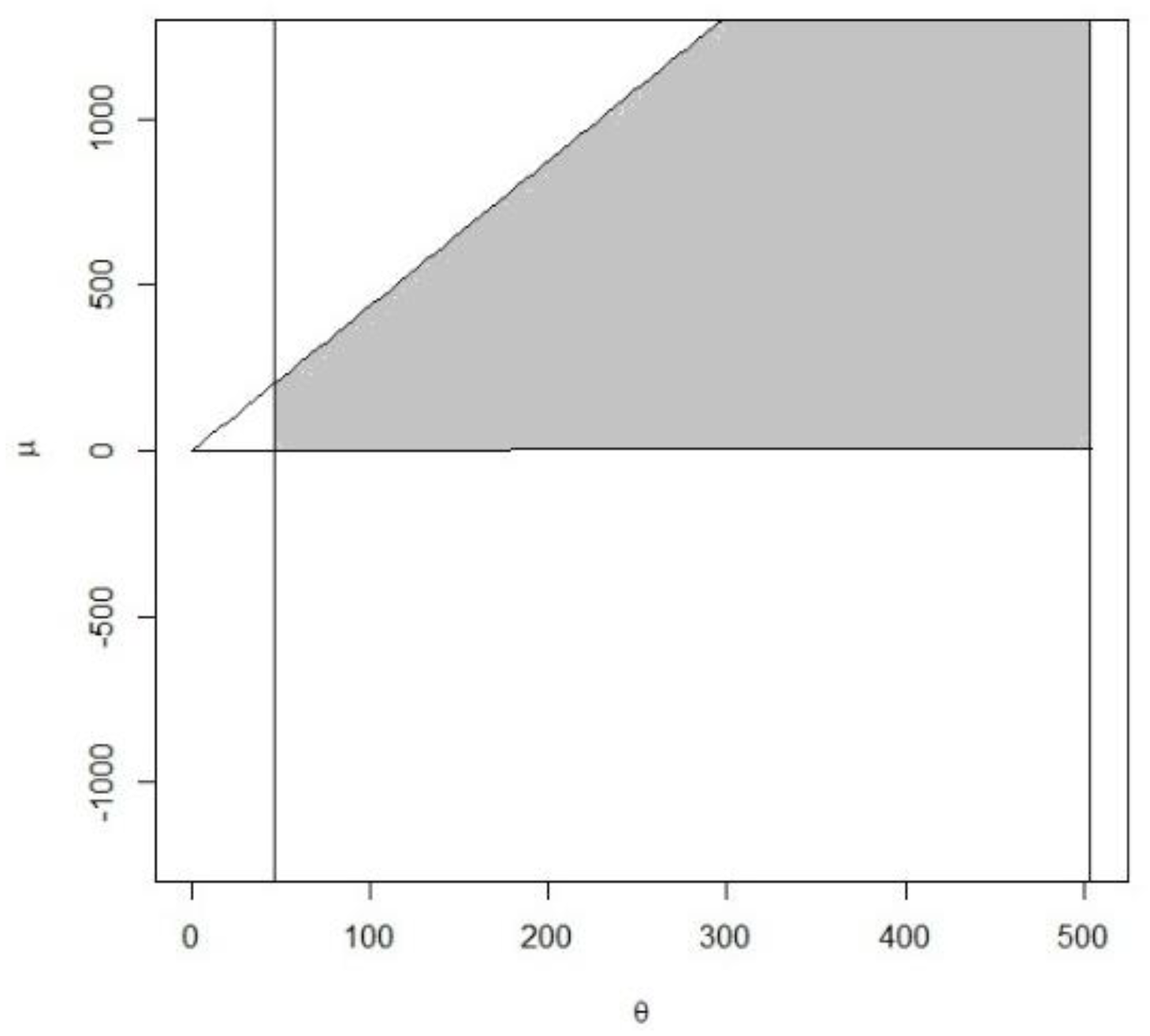
Under a = 2 and b = 2, by Theorem 1, the 95% credible confidence interval for is obtained as (0.75123, 1.2384) with a confidence length of 0.4872, which is smaller than the confidence length of 0.5836 reported by Wu [9]. By Theorem 2 (Method 1), with a = 2 and b = 2, the 95% credible joint confidence region displayed in Figure 1 for is given by
with an area of 231,528.4.
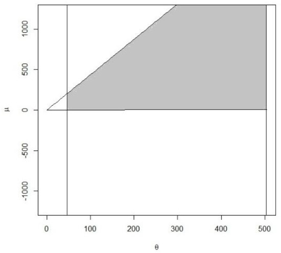
Figure 1.
The 95% credible confidence region under Method 1.
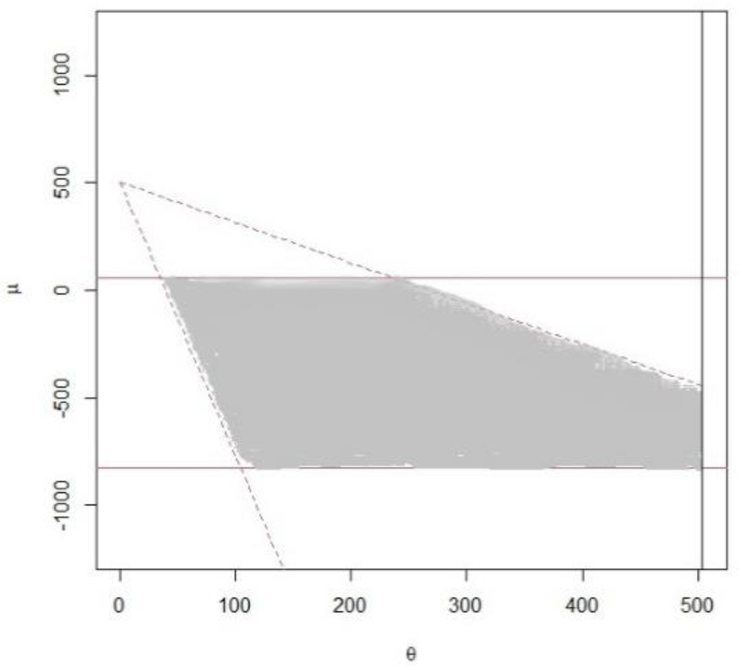
Applying Theorem 3 (Method 2), the confidence region displayed in Figure 2 is given by with an area of 12,021.83. In this case, Method 2 has smaller area than Method 1. For the development of the 95% Bayesian prediction interval for the future upper record value , Theorem 4 is applied. The 95% Bayesian prediction interval for is given by (504.2641, 988.7105).
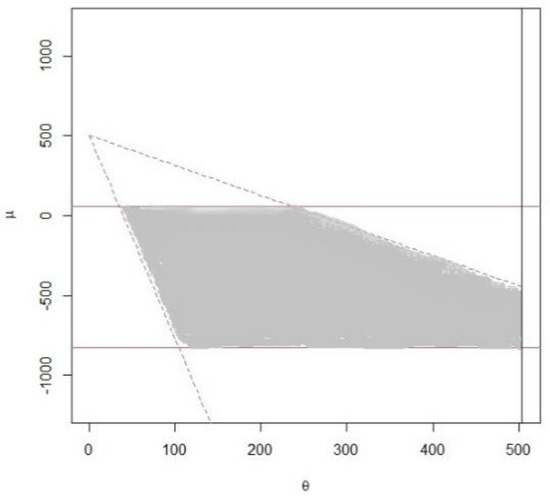
Figure 2.
The 95% credible confidence region under Method 2.
6. Conclusions
In this study, we propose a Bayesian credible interval for the scale parameter and introduced two Bayesian approaches, Method 1 and Method 2, to obtain the credible region for the two parameters of the two-parameter exponential distribution using upper record value data. In addition, a Bayesian prediction interval for the future upper record value is developed. A simulation study is conducted to compare the Bayesian methods with the non-Bayesian approach proposed by Wu [9], considering various sample sizes and different parameter setups for a and b in the Bayesian methods. With respect to confidence lengths and region areas, the Bayesian method performs better for most cases. In terms of coverage probabilities, the simulation results show that the Bayesian method with parameters a = 2 and b = 2 achieves a higher coverage probability than the non-Bayesian method for interval estimation of the scale parameter. For the credible region, Method 2, with parameters a = 2 and b = 2, demonstrates a higher coverage probability compared to the other Bayesian method and the non-Bayesian method. For the prediction interval, the Bayesian method with a = 2 and b = 2 also achieves a higher coverage probability. Consequently, the Bayesian method with these parameter settings is recommended for practical applications. Finally, an engineering example is presented to illustrate all the proposed Bayesian methods for the two-parameter exponential distribution using upper record value data.
Funding
This research and the APC were funded by [National Science and Technology Council, Taiwan] NSTC 113-2118-M-032-002-.
Data Availability Statement
Data are available in a publicly accessible repository. The data presented in this study are openly available in Proschan [13].
Conflicts of Interest
The authors declare no conflicts of interest.
References
- Johnson, N.L.; Kotz, S.; Balakrishnan, N. Continuous Univariate Distributions; Wiley: New York, NY, USA, 1994. [Google Scholar]
- Bain, L.J.; Engelhardt, M. Statistical Analysis of Reliability and Life Testing Models; Marcel Dekker: New York, NY, USA, 1991. [Google Scholar]
- Lawless, J.E. Statistical Models and Methods for Lifetime Data, 2nd ed.; John Wiley and Sons Inc.: New York, NY, USA, 2003. [Google Scholar]
- Afolabi, A.M.; OKE, I.I. Exponential Probability Distribution of Short-Term Rainfall Intensity. Equity J. Sci. Technol. 2022, 9, 18–27. [Google Scholar]
- Douglas, E.S.V.; Dayana, E.W.S.; Luiz, G.D.A.A.; Ricardo, A.; Nilo, A.D.S.S. Application of the exponential distribution to improve environmental quality in a company in the south of Rio de Janeiro State. Rev. Gestão Secr. 2023, 14, 15695–15704. [Google Scholar]
- Zhang, Y.; Wang, S.; Ke, X.; Ye, H. A new Kolmogorov-Smirnov test based on representative points in the exponential distribution family. J. Stat. Comput. Simul. 2024, 94, 3391–3408. [Google Scholar] [CrossRef]
- Arnold, B.C.; Balakrishnan, N.; Nagaraja, H.N. Records; John Wiley & Sons, Inc.: New York, NY, USA, 1998. [Google Scholar]
- AL-Hussaini, E.K.; Ahmad, A.A. On Bayesian Interval Prediction of Future Records. Test 2003, 12, 79–99. [Google Scholar] [CrossRef]
- Wu, S.F. Interval estimation for the two-parameter exponential distribution based on the upper record values. Symmetry 2022, 14, 1906. [Google Scholar] [CrossRef]
- Barde, S. Bayesian estimation of large-scale simulation models with Gaussian process regression surrogates. Comput. Stat. Data Anal. 2024, 196, 107972. [Google Scholar] [CrossRef]
- Sundaram, P.S.; Radha, R.K.; Venkatesan, P. Bayesian estimation of Weibull-G-Weibull distribution for censored data using M-H algorithm. Adv. Appl. Stat. 2024, 91, 1095–1112. [Google Scholar] [CrossRef]
- Wu, S.F. Interval estimation for the two-parameter exponential distribution under progressive type II censoring on the Bayesian approach. Symmetry 2022, 14, 808. [Google Scholar] [CrossRef]
- Proschan, F. Theoretical explanation of observed decreasing failure rate. Technometrics 1963, 3, 375–383. [Google Scholar] [CrossRef]
Disclaimer/Publisher’s Note: The statements, opinions and data contained in all publications are solely those of the individual author(s) and contributor(s) and not of MDPI and/or the editor(s). MDPI and/or the editor(s) disclaim responsibility for any injury to people or property resulting from any ideas, methods, instructions or products referred to in the content. |
© 2024 by the author. Licensee MDPI, Basel, Switzerland. This article is an open access article distributed under the terms and conditions of the Creative Commons Attribution (CC BY) license (https://creativecommons.org/licenses/by/4.0/).