A Gaussian Process-Enhanced Non-Linear Function and Bayesian Convolution–Bayesian Long Term Short Memory Based Ultra-Wideband Range Error Mitigation Method for Line of Sight and Non-Line of Sight Scenarios

Abstract

Relative positioning accuracy between two devices is dependent on the precise range measurements. Ultra-wideband (UWB) technology is one of the popular and widely used technologies to achieve centimeter-level accuracy in range measurement. Nevertheless, harsh indoor environments, multipath issues, reflections, and bias due to antenna delay degrade the range measurement performance in line-of-sight (LOS) and non-line-of-sight (NLOS) scenarios. This article proposes an efficient and robust method to mitigate range measurement error in LOS and NLOS conditions by combining the latest artificial intelligence technology. A GP-enhanced non-linear function is proposed to mitigate the range bias in LOS scenarios. Moreover, NLOS identification based on the sliding window and Bayesian Conv-BLSTM method is utilized to mitigate range error due to the non-line-of-sight conditions. A novel spatial–temporal attention module is proposed to improve the performance of the proposed model. The epistemic and aleatoric uncertainty estimation method is also introduced to determine the robustness of the proposed model for environment variance. Furthermore, moving average and min-max removing methods are utilized to minimize the standard deviation in the range measurements in both scenarios. Extensive experimentation with different settings and configurations has proven the effectiveness of our methodology and demonstrated the feasibility of our robust UWB range error mitigation for LOS and NLOS scenarios.

1. Introduction

Accurate positioning is one of the main courses of research in various engineering fields, and it has received a lot of attention in recent years owing to its inherent academic importance [1,2]. Applications across a wide range of industries, including telecommunications, intelligent machines, and medical/rescue operations, might greatly benefit from this technology, as could autonomous driving [3,4,5]. Despite this, precise location in line-of-sight (LOS) and non-line-of-sight (NLOS) scenarios for indoor environments remains a research challenge. Multipath effects, reflections, refractions, and other propagation events can cause errors in the location estimate process [6,7].

Localization has been accomplished via various technologies, such as sensor nodes, acoustics, simultaneous localization and mapping, inertial measurement units, and ultra-wideband (UWB) communications. UWB is a potential technology for accurate positioning because of a variety of desired qualities, namely low energy consumption, centimeter-level range accuracy, susceptibility to multipath effects, and a certain obstacle penetrating capacity [8]. UWB has been intensively studied in recent years by academics and industry for indoor and relative positioning [9,10]. On the other hand, the precision of UWB localization degrades when the signal propagates through the obstruction and is subject to antenna calibration issues, and NLOS situations result in a positive bias in range measurements. Most of the UWB-based localization technology uses Time Difference of Arrival (TDoA), Time of Arrival (TOA), and two-way ranging (TWR) methods. The TWR methods are the most common and robust methods because no anchor synchronization is needed to get precise ranging measurements.

TWR is very significant when clock synchronization is not obtainable or not used in a positioning method. The distance between two devices is calculated by measuring the Time of Flight (ToF) between them. Instead of utilizing direct timestamps, the TWR technique calculates the distance between two devices using a sequence of time intervals. This is due to the fact that the duration of a particular time is the same across all devices, independent of their individual clock references. However, a clock will drift from its original state even if it is properly calibrated due to the inherent faults of clock oscillators in the actual physical world [11]. These clock drifts result in inaccurate measurements of the time periods given, particularly whenever the application needs centimeter-level precision. This is because a 1 ns ToF inaccuracy may result in a range measurement error of 30 cm [12]. As a result, various TWR approaches exist in the literature to reduce the inaccuracy in range caused by clock drifts. One of the best and most used methods is the asymmetric TWR method, which reduces errors due to clock and frequency drift. However, the asymmetric TWR method also has an error due to antenna delay and NLOS conditions.

The term “NLOS” generally refers to a scenario in which the direct route between a transceiver and a receiver is impeded. Consequently, the signals travel via a penetrated, reflected, or diffracted route before reaching the receiver, increasing the travel time and decreasing signal intensity. As a result, the distance calculated using either time or signal strength is affected. NLOS is a prevalent issue with wireless positioning technologies, including WiFi, ZigBee, Bluetooth, and UWB. Compared to other approaches, UWB presents a more serious difficulty due to its operating range and the needed precise indoor or relative positioning [13]. As a result, NLOS detection and mitigation has become a major topic in the area of UWB-based positioning systems [14]. Most of the proposed NLOS mitigation methods in the research involve likelihood ratio tests, channel impulse response (CIR)-based techniques, and machine learning algorithms. Moreover, the recent literature has proposed support vector machines, Gaussian processes, deep learning, and representation learning models to mitigate NLOS effects. However, to mitigate range error in LOS and NLOS conditions, different parameters such as antenna delay and NLOS environment characteristics play a vital role in mitigating range error. These approaches generally mitigate the LOS- or NLOS-induced range measurement errors before positioning or mitigate the influence of range errors using specific positioning techniques. Although it is commonly understood that perfect range error mitigation is impossible, these solutions ignore the impact of residual range errors and antenna delay calibration on positioning. Furthermore, current NLOS detection and mitigation approaches classify the propagation state as either LOS or NLOS without further information about the NLOS’s characteristics. We present a novel range error mitigation method for both LOS and NLOS conditions before the positioning to address these issues. The following are the primary contributions of this paper:

• A GP-enhanced non-linear function and exponential moving average and min-max removing algorithms are proposed to mitigate range bias in the LOS environment.
• A Conv-BLSTM deep learning model-based NLOS identification method is proposed to identify the NLOS propagation through different materials for indoor environments, such as wood, the human body, concrete walls, and metals.
• A novel spatial–temporal attention module is proposed to effectively process the data’s features.
• The Monte Carlo (MC) dropout-based uncertainty estimation model is introduced to estimate the proposed model’s uncertainty to demonstrate the proposed model’s robustness.

The rest of the paper is structured as follows: Section 2 presents the related works associated with this research, Section 3 describes the data preparation method for the proposed algorithms, Section 4 presents the proposed algorithms to mitigate range bias in LOS and NLOS scenarios, Section 5 describes the experimental setting and a discussion on the results, and the conclusion is drawn in Section 6.

2. Related Works

This section divides the existing range error mitigation into two categories based on the LOS and NLOS environments. LOS error mitigation includes antenna calibration, power calibration, and bias compensation due to radio signal strength. The second category involves identifying the NLOS situation and range error mitigation to enable precise range measurement.

2.1. LOS Range Error Mitigation

LOS range error sources include clock drift, power calibration, antenna delay, and bias caused by the signal power. Several approaches are found in the literature to correct clock drift in the UWB-range measurement devices. Fofana et al. developed a dynamic correction methodology that uses artificial delay between messages to calculate clock drift coefficients, which is utilized to limit clock drift in the two-way ranging method. The authors obtained an accuracy of twenty millimeters, enabling range traffic to be included in regular traffic [15]. Adrien et al. developed an open-source framework called Decaduino to enable range measurement using UWB chips. The authors used delay transmission and introduced artificial delay between messages through UWB devices. The authors achieved 15 cm accuracy in range measurements, which is very precise compared to other wireless range measurement technologies [16]. Martel et al. introduced a digital low pass filter to correct clock skew evaluation during TWR range measurements. The proposed method achieves very good results, with an 18 cm mean error and 1.77 cm standard deviation in range measurements [17]. Dotlic et al. proposed three calculating approaches for significantly minimizing systematic localization mistakes caused by clock offsets in comparable localization systems with a low frame exchange rate. The error reduction mechanism is based on the receiver’s carrier frequency offset estimation, which is a necessary component of frame reception in many UWB-based systems [18]. Decawave instructed calibrating the antenna and power spectrum of the Decawave’s DW1000 chips, but their calibrating method must be implemented manually, which is a big constraint for real-time and commercial applications [12]. Qiang et al. proposed Kalman filter-based range bias estimation and mitigation for both LOS and NLOS environments [19]. Their approach achieves good results by reducing the error to a millimeter level; however, the Kalman filter is computationally expensive for small microcontroller devices and is not suitable for energy-constrained devices. Therefore, a new antenna calibration method and bias mitigation method should be implemented to enable real-time application.

2.2. NLOS Range Error Mitigation

NLOS range error mitigation for UWB-based solutions includes effective NLOS identification and NLOS range bias mitigation. Traditional NLOS identification methods can be divided into range, location, and channel-based methods [20,21]. Range-based approaches employ the probability density function (PDF) or variation of range estimations to differentiate LOS from NLOS [21] conditions. Channel-based approaches distinguish NLOS from LOS by utilizing CIR, which is accomplished via the use of two widely used functions, the PDF and the cumulative distribution function (CDF) [22]. However, determining a suitable distribution function and determining the proper threshold can be difficult [23]. It is also uncertain how to establish the threshold. Location-based approaches detect NLOS conditions during the location estimate process and might utilize the obtained location information to identify NLOS conditions. The location-based approach is expected to be useful in the scenario wherein redundant range estimates are accessible since it compares the location estimates provided with various sets of range estimations [24], but it is useless when there are no redundant range estimates or when numerous range estimates correspond to NLOS conditions. In order to solve the above-mentioned issues, researchers used different machine learning approaches for NLOS identification. Henk et al. proposed support vector machines to detect non-line-of-sight conditions and mitigate range error in the non-line-of-sight environment [25]. Nguyen et al. introduced relevance vector machine algorithms to mitigate range error in non-line-of-sight environments [26]. Sang et al. used different available machine learning techniques to identify the NLOS and multipath conditions in an indoor environment and compare the performance of the different machine learning algorithms [27]. However, one thing should be noted: wireless signal propagation is different in different materials, and most researchers did not consider these facts.

3. Data Preparation

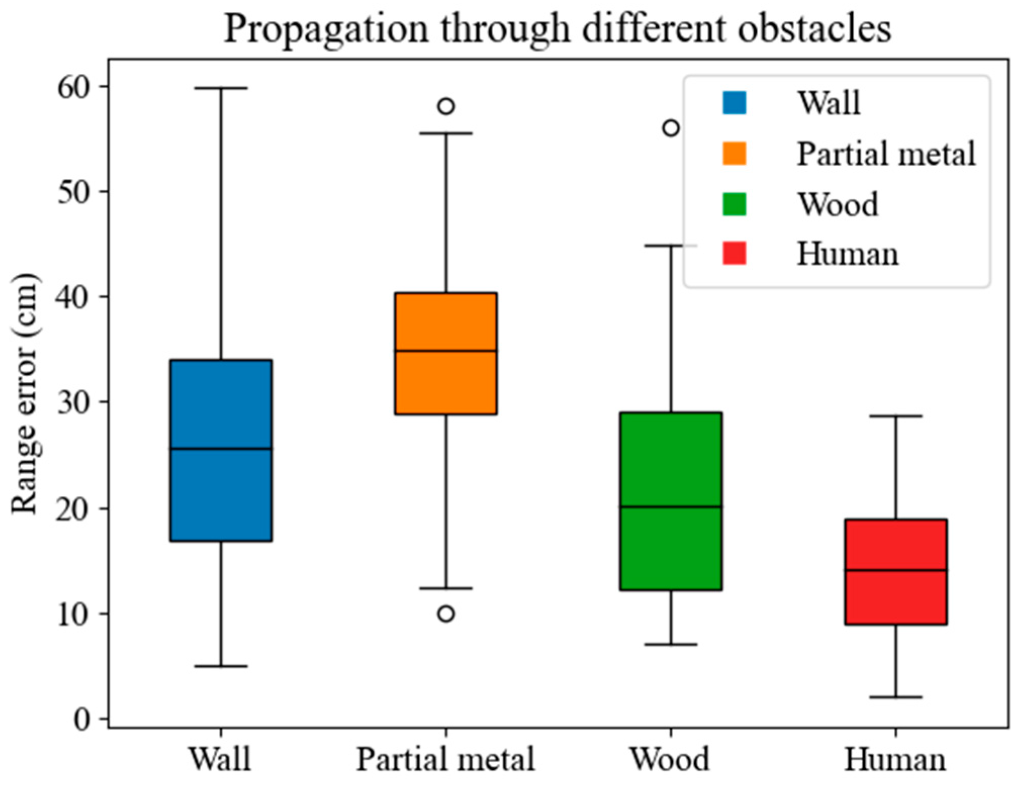
The range measurements were done in five distinct locations to cover a broad range of LOS and NLOS scenarios: a wide-space area where the obstacles were metal, a human body obstacle between an anchor and a tag [28], an indoor office area where the obstacles were wood, and concrete walls as obstacles. Furthermore, additional measurements were taken across several rooms to investigate the through-the-wall impact. Figure 1 shows the box chart range error of different common obstacles found in the indoor environment. We can see that the propagation through the wall and partial metal obstacles induced large range error compared to the propagation through the wood and human obstacles. Due to the nature of the obstacles and radio signals, range error information from different propagation channels can be beneficial to mitigate the range error for different environments. Therefore, range measurements were taken under various conditions, which can be used to mitigate range error across different environments and allow a representation learning approach to acquire a domain-independent model.

Figure 1. Range measurement error represented in the box chart for four different NLOS propagation scenarios, which can be found indoors. The square box represents the mean, and the dashes represent the maximum and minimum range error observed during the data acquisition.

We utilized an embedded Decawave DW1000 (Qorvo Inc., Greensboro, NC, USA) UWB chip with a NodMCU-BU01 module. As ground truth, a measurement ruler was used to measure the precise distance between the anchor and the tag. To produce both LOS and NLOS data, the tag was placed in different environments loaded with obstacles.

Figure 1 shows the boxplot range error for different propagation scenarios in our acquired data. It can be seen that the range error is very high during partial metal propagation. The mean range error also varies for different propagation materials.

4. Materials and Methods

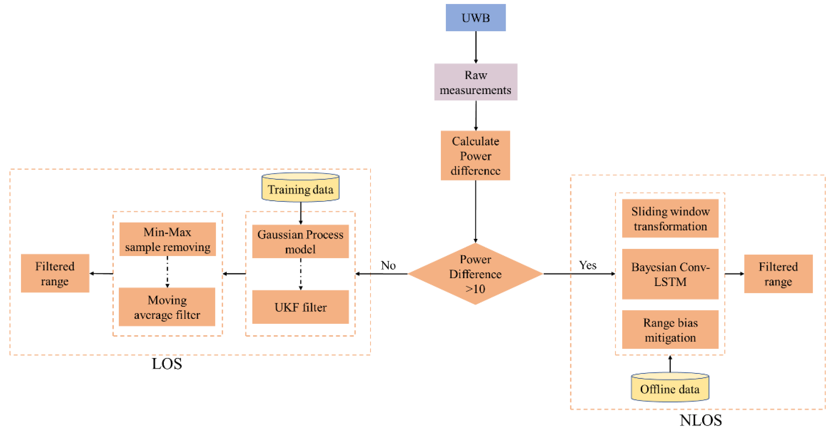
In this section, we propose the range error mitigation of UWB devices for both LOS and NLOS environments. We propose a Gaussian process model and an unscented Kalman filter along with min-max removing, and a moving average filter is used to reduce the standard deviation of the acquired LOS range measurement. The NLOS identification for different obstacles and NLOS range error mitigation model was developed using the deep learning method. Since the UWB devices are low-power and energy-constrained devices connected to the microcontroller module, the range error mitigation method must be implemented in the microcontroller or edge devices to provide real-time range error mitigation before calculating the positioning. This study mainly focuses on implementing the proposed method in low-level microcontroller devices to minimize inference time and latency. The overall structure of the proposed range error mitigation of the UWB module can be seen in Figure 2.

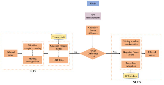
Figure 2. The overall system architecture of the proposed UWB range measurement error mitigation for both LOS and NLOS environments.

4.1. LOS Range Mitigation

4.1.1. System Model

We consider an asynchronous Double-Sided (DS)-TWR UWB system comprising two nodes: a transmitter (Tx) and a receiver (Rx). The range measurement process involves the exchange of UWB signals, with the Time of Flight (ToF) of the signals being critical for range estimation. The ToF, denoted as $T_{\mathrm{ToF}}$, is the time taken by the UWB signal to travel from the Tx to the Rx. In an ideal scenario without any errors, the true range R between the nodes is related to $T_{\mathrm{ToF}}$ by

$$R=c\times T_{\mathrm{ToF}},$$

(1)

where c is the speed of light.

The actual measured ToF, denoted as $T_{\mathrm{ToF}}^{\prime }$, is affected by various errors, such as environmental noise ($N_{\mathrm{env}}$). This includes multipath effects, interference from other signals, and atmospheric conditions. Chip imperfections ($N_{\mathrm{chip}}$) include errors due to hardware imperfections in the UWB transceivers. Antenna delay (${\delta }_{\mathrm{ant}}$) includes the inherent delay in the Tx and Rx antennas. The observed ToF can thus be modeled as

$$T_{\mathrm{ToF}}^{\prime }=T_{\mathrm{ToF}}+{\displaystyle \frac{N_{\mathrm{env}}+N_{\mathrm{chip}}+{\delta }_{\mathrm{ant}}}{c}}$$

(2)

4.1.2. Problem Formulation

The objective is to accurately estimate the true range R from the observed $T_{\mathrm{ToF}}^{\prime }$ while mitigating the errors. The estimation problem can be formulated as follows:

• Range estimation with error mitigation: we have to find an estimator $\widehat{R}$ such that

  $$\widehat{R}={\mathrm{argmin}}_R\mathbb{E}\left[{\left(R-\left(c\times T_{\mathrm{ToF}}^{\prime }\right)\right)}^2\right]$$

  (3)

  where $\mathbb{E}[\cdot ]$ denotes the expectation operator, signifying the minimization of the mean squared error between the true range and the estimated range.
• Error correction modeling: we can model the combined errors as a stochastic process, which can be learned and predicted:

  $$N_{\mathrm{total}}=N_{\mathrm{env}}+N_{\mathrm{chip}}+{\delta }_{\mathrm{ant}}$$

  (4)
  Using a Gaussian process model, we can correct initial range as follows:

  $$R_{\mathrm{GP}}=c\cdot \left(T_{\mathrm{ToF}}^{\prime }-{\displaystyle \frac{\mathcal{G}\mathcal{P}\left(m\left(T_{\mathrm{ToF}}^{\prime }\right),k\left(T_{\mathrm{ToF}}^{\prime },T_{\mathrm{ToF}}^{″}\right)\right)}{c}}\right)$$

  (5)

  where $GP\left(m,k\right)$ directly models the $N_{\mathrm{total}}$ as a function of observed $T_{\mathrm{ToF}}^{\prime }$, using a mean function $m$ and a covariance function $k$ that learns from historical data of $T_{\mathrm{ToF}}^{\prime }$ and the total error.

The initial correction from the GP model can be fine-tuned using a statistical filter by incorporating dynamic system behavior and residual error correction as follows:

$$\widehat{R}=c\cdot \left(\mathcal{U}\mathcal{K}ℱ\left(X_{k\mid k-1}^{\left(i\right)}\right)-{\displaystyle \frac{{\widehat{N}}_{\mathrm{resediual}}}{c}}\right)$$

(6)

where $\widehat{R}$ denotes the final corrected range estimate. The UKF considered the state represented by sigma points $X_{k\mid k-1}^{\left(i\right)}$, which have been adjusted from the $R_{\mathrm{GP}}$. The residual error ${\hat{N}}_{\mathrm{residual}}$ includes those components of $N_{\mathrm{total}}$ not mitigated by the initial GP correction.

4.1.3. Proposed Method

The GPA-UKF method is designed to enhance the accuracy of ultra-wideband (UWB) range measurements, which are often subject to errors due to antenna delays and environmental factors. The method synergizes the state estimation capabilities of the UKF with the error correction proficiency of GP models. This integration mitigates the non-linear and uncertain nature of UWB systems, yielding a more accurate and reliable range estimation.

A GP model is first utilized to predict and correct the total error ($N_{\mathrm{total}})$ affecting the ToF measurements. This total error encompasses various sources, including environmental noise ($N_{\mathrm{env}}$), chip imperfections ($N_{\mathrm{chip}}$), and antenna delay (${\delta }_{\mathrm{ant}}$).

A Gaussian process can be defined using mean function $m\left(x\right)$ and covariance function $k\left(x,x^{\prime }\right)$, where $x$ and $x^{\prime }$ represent points in the input space, such as $T_{\mathrm{ToF}}^{\prime }$ as follows:

$$\begin{array}{l}m\left(x\right)=\mathbb{E}\left[f\left(x\right)\right]\\ k\left(x,x^{\prime }\right)=\mathbb{E}\left[\left(f\left(x\right)-m\left(x\right)\right)\left(f\left(x^{\prime }\right)-m\left(x^{\prime }\right)\right)\right]\end{array}$$

(7)

The GP model, denoted as $GP\left(m,k\right)$, captures the distribution over the possible functions $f\left(x\right)$ that fit the observed data. In our scenario, the function $f$ predicts the total error $N_{\mathrm{total}}$ as a function of the observed $T_{\mathrm{ToF}}^{\prime }$. The GP model learns the function $f$ that maps $T_{\mathrm{ToF}}^{\prime }$ to $N_{\mathrm{total}}$. This learning process involves maximizing the likelihood of the observed data under the GP model as follows:

$$ℒ\left(\theta \mid T_{\mathrm{ToF}}^{\prime },N_{\mathrm{total}}\right)=\log p\left({\mathit{N}}_{total}\mid {\mathit{T}}_{ToF}^{\prime },\theta \right)$$

(8)

where $\theta$ represents the GP hyperparameters, and $T_{\mathrm{ToF}}^{\prime }$ and $N_{\mathrm{total}}$ are vectors of observed ToF measurements and their corresponding error.

The trained GP model can predict the error ${\hat{N}}_{\mathrm{total}}$ for a new ToF measurement, $T_{\mathrm{ToF}}^{\prime }$. The initial range correction is then performed by adjusting the observed ToF for the predicted error as follows:

$$R_{\mathrm{GP}}=c\cdot \left(T_{\mathrm{ToF}}^{\prime }-{\displaystyle \frac{GP\left(m\left(T_{\mathrm{ToF}}^{\prime }\right),k\left(T_{\mathrm{ToF}}^{\prime },T_{\mathrm{ToF}}^{″}\right)\right)}{c}}\right)$$

(9)

where $R_{\mathrm{GP}}$ is the initial corrected range measurement.

The UKF, known for its efficacy in non-linear systems, is employed to fine-tune the initial correct range measurements from the GP model, considering the system’s dynamics and measurement noise. We can first define a state transition function as below:

$$x_{k+1}=f\left(x_k,w_k\right)$$

(10)

where $x_k$ denotes the state at time k, f is the non-linear state transition function, and $w_k$ represents the process noise.

We utilize sigma points to approximate the distribution of the system’s state. Sigma points are selected to represent the possible states of the system. They are determined around the current state estimate and spread according to the state covariance. Mathematically, for a state vector x of dimension n, the sigma points $X^{\left(i\right)}$ are computed as follows.

$$\begin{array}{l}{X}^{\left(0\right)}=\overline{x}\\ X^{\left(i\right)}=\overline{x}+{(\sqrt{\left(n+\lambda \right)P})}_i\mathrm{for}i=1,\dots ,n\\ X^{\left(i\right)}=\overline{x}-{(\sqrt{\left(n+\lambda \right)P})}_{i-n}\mathrm{for}i=n+1,\dots ,2n\end{array}$$

(11)

where $\overline{x}$ is the mean state estimate, P is the state covariance matrix, λ is a scaling parameter, and $\sqrt{\left(n+\lambda \right)P}{)}_i$ represents the ith column of the matrix square root of (n + λ) P. These sigma points are then propagated through the non-linear state transition function f and measurement function h:

$$\begin{array}{l}{X}_{k\mid k-1}^{\left(i\right)}=f\left(X_{k-1\mid k-1}^{\left(i\right)},w_{k-1}\right)\\ Z_k^{\left(i\right)}=h\left(X_{k\mid k1}^{\left(i\right)},v_k\right)\end{array}$$

(12)

where $X_{k\mid k-1}^{\left(i\right)}$ are the propagated sigma points through the state transition, and $Z_k^{\left(i\right)}$ are the sigma points transformed by the measurement function.

$${\overline{x}}_{k\mid k}={\displaystyle \sum }_{i=0}^{2n}{W}_i^{\left(m\right)}{X}_{k\mid k-1}^{\left(i\right)}$$

(13)

$$P_{k\mid k}={\displaystyle \sum }_{i=0}^{2n}{W}_i^{\left(c\right)}\left(X_{k\mid k-1}^{\left(i\right)}-{\overline{x}}_{k\mid k}\right){\left(X_{k\mid k-1}^{\left(i\right)}-{\overline{x}}_{k\mid k}\right)}^T$$

(14)

where $W_i^{\left(m\right)}$ and $W_i^{\left(c\right)}$ are weights for the mean and covariance, respectively.

The Kalman gain, $K_k$, is then computed to update the state estimate with the measurement $Z_k:$

$$\begin{array}{l}{K}_k=P_{k\mid k-1}^z{\left(P_{k\mid k-1}^{ϵ}\right)}^{-1}\\ {\overline{x}}_{k\mid k}={\overline{x}}_{k\mid k-1}+K_k\left(Z_k-{\overline{Z}}_k\right) \\ P_{k\mid k}=P_{k\mid k-1}-K_k{P}_{k\mid k-1}^z{K}_k^T\end{array}$$

(15)

where $P_{k\mid k-1}^z$ is the covariance of the predicted measurement, and $P_{k\mid k-1}^{ϵ}$ is the measurement noise covariance.

The initial state of the UKF ${\overline{x}}_0$ is adjusted based on the corrected range from the GP model output $R_{\mathrm{GP}}$ as follows:

$${\overline{x}}_0^{adj}={\overline{x}}_0+K_{\mathrm{GP}}\cdot \left(R_{\mathrm{GP}}-H\cdot {\overline{x}}_0\right)$$

(16)

where $K_{\mathrm{GP}}$ is an adjustment factor on the initial state estimation, $H$ is the measurement matrix relating the state to the measured range, and ${\overline{x}}_0^{adj}$ denotes the adjusted initial state.

The final measurement update of the system is then calculated as follows:

$${\hat{R}}_{k\mid k}=c\cdot \left(\mathcal{U}\mathcal{K}ℱ\left(X_{k\mid k-1}^{\left(i\right)}\right)-{\displaystyle \frac{{\hat{N}}_{\mathrm{residual},k}}{c}}\right)$$

(17)

where ${\hat{R}}_{k\mid k}$ is the dynamically refined range estimate at time step $k$, incorporating the continuous adjustments for residual errors (${\hat{N}}_{\mathrm{residual},k}$) identified through the UKF process after the initial GP corrections.

4.2. NLOS Range Mitigation

4.2.1. System Model

The range measurement in an NLOS environment at time $t_k$ is affected by the nature of the obstruction. The model is expressed as

$$d_{\mathrm{NLOS}}=d+\mathsf{\Delta }{d}_{\mathrm{nlos}}\left(\mathrm{obstacle},t_k\right)+\epsilon$$

(18)

where $d_{\mathrm{NLOS}}$ is the observed distance, d is the actual line-of-sight distance, $\mathsf{\Delta }{d}_{\mathrm{nlos}}$ represents the range error influenced by the type of obstacle, and ε signifies the combined standard deviation and mean error. The nature of the obstacle influences the NLOS range bias, $\mathsf{\Delta }{d}_{\mathrm{nlos}}$. For example, concrete walls and metal cause significant reflections and absorption of UWB signals, leading to large-range errors. Wood and partial obstructions result in less severe but still notable attenuation and multipath effects. The presence of people affects the signal due to absorption and reflection, introducing variability in range measurements. The range error due to NLOS conditions is thus a function of the obstacle type and the measurement duration:

$$\mathsf{\Delta }{d}_{\mathrm{nlos}}=f_{\mathrm{obstacle}}\left(d,\mathrm{type},t_k\right)$$

(19)

4.2.2. Problem Formulation

The goal is to develop an estimation process that adapts to the variability introduced by different obstructions, accurately estimating the true range in diverse NLOS conditions. An estimator ${\widehat{d}}_{\mathrm{NLOS}}$ is required that minimizes the error across various types of obstructions:

$${\widehat{d}}_{\mathrm{NLOS}}={\mathrm{argmin}}_d\mathbb{E}\left[{\left(d-\left(d+\Delta d_{\mathrm{nlos}}\left(obstacle,t_k\right)+\epsilon \right)\right)}^2\right]$$

(20)

The error model needs to characterize the distinct impacts of different materials on signal propagation. This involves analyzing the impact of different materials uniquely affecting UWB range measurements:

$$\mathsf{\Delta }{d}_{\mathrm{nlos}}\left(\mathrm{obstacle},t_k\right)=g_{\mathrm{material}}\left(d,\mathrm{type},t_k,\epsilon \right)$$

(21)

where $g_{\mathrm{material}}$ models the NLOS error based on the type of obstruction, time, and inherent measurement errors.

4.2.3. Proposed Method

1. Sliding window function: the sliding window function is a batch estimation technique requiring constant time and memory since it marginalizes older states [14,15]. Consider the case wherein a device travels until time t_k1, at which point it can be understood to be in an NLOS state by doing a thorough batch estimate of its state history. It then travels until time t_k2, at which point it adds the new state to its state history. The previous state m is then marginalized out of the optimization problem being addressed at t_k2, thereby eliminating them from the challenge. The new states are the remaining states from the preceding window’s estimation. The sliding window function is normally used to process time-series data in machine learning and deep learning models. As the UWB device goes from an LOS to NLOS state at different timeslots, we need to use the sliding window function to utilize time-series data to estimate the state of the UWB device at time t_k1.

$$\underset{︷}{\mathrm{new}\mathrm{window}\mathrm{of}\mathrm{length}K=k_2-m+1}$$

(22)

$$\underset{ \mathrm{old}\mathrm{window}\mathrm{of}\mathrm{length}K=k_1+1}{\overset{x_0 x_1 \dots x_{m-1} x_m \dots x_{k_1}}{︸}} x_{k_1+1} \dots x_{k_2}$$

(23)

where every state can be represented as an LOS or NLOS state. The Decawave DW1000 UWB chip user manual stated that if the difference between RX_POWER and FP_POWER, i.e., RX_POWER − FP_POWER, is less than 6 dB, the channel is likely to be LOS, based on the thumb rule. Therefore, every state is compared with the defined RX_POWER − FP_POWER = 6 dB value to first differentiate the LOS state from the NLOS state, then machine learning algorithms are used on the NLOS state data to identify the characteristics of the NLOS propagation.

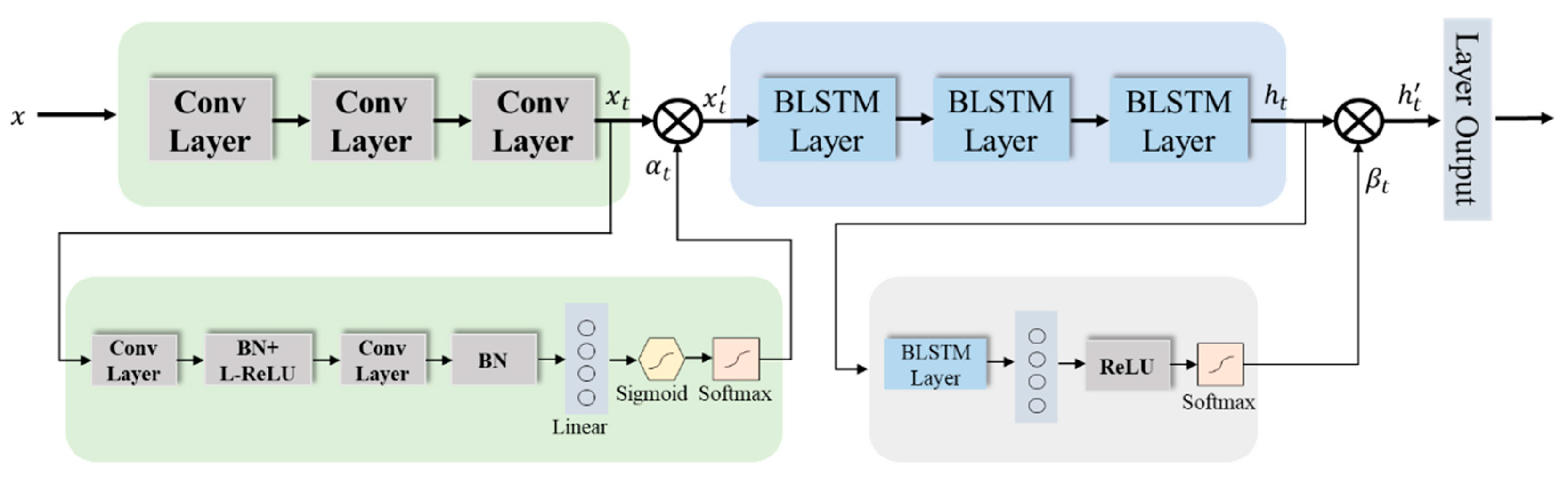
2. Bayesian Conv-LSTM: this study utilizes the cascade of convolution and Bayesian LSTM to classify the NLOS scenarios with high accuracy. Figure 3 shows the overall structure of the proposed method with the attention module. The input data first pass through the convolution layer and then pass through the Bayesian LSTM (BLSTM) layer, followed by the layer output with the softmax activation function to classify the input. A novel spatial–temporal attention module is proposed to extract important input features, improving the model’s performance. The spatial attention is placed at the convolution layer’s end, and the temporal attention module is placed at the end of the Bayesian LSTM layer to extract important features. A detailed description of the BLSTM layer and the proposed attention module is presented in this section.

Figure 3. The overall architecture of Conv-BLSTM layer and the proposed attention module.

Bayesian inference in deep learning allows mathematically grounded uncertainty estimation, which can improve the model performance. Grahmani et al. proposed dropout with variational inference to estimate uncertainty in the deep learning model [29]. The uncertainties in the deep learning model can be divided into epistemic and aleatoric uncertainty. The epistemic uncertainty accounts for the lack of a dataset, which can be reduced by providing more observable data to the models during training. The aleatoric uncertainty accounts for the randomness of the data during the acquisition, which cannot be reduced. Moreover, the aleatoric uncertainty can be divided into two parts, such as homoscedastic and heteroscedastic. The homoscedastic uncertainty provides a constant uncertainty estimation regardless of different data points. On the other hand, the heteroscedastic uncertainty varies according to the input data, which is very useful in understanding the noise variance during data acquisition. Therefore, this study considers the epistemic and heteroscedastic aleatoric uncertainty estimation to determine the proposed model’s uncertainties in predicting the NLOS class.

A Bayesian neural network replaces the deterministic weights’ parameters with a distribution using the Bayesian rule. For example, the posterior over deep learning weights for a given dataset (X, Y) can be defined as $p\left(W|X,Y\right)$ in a Bayesian neural network. We can also derive the model likelihood, which contains Gaussian observation noise as follows:

$$p\left(y|f^w\left(x\right)\right)=N\left(f^w\left(x\right),{\sigma }^2\right),$$

(24)

where $f^w$ represents the random output from a Bayesian neural network, and $\sigma$ represents the Gaussian observation noise. However, it is known that the exact posterior of the Bayesian neural network is intractable, but it can be approximated using different approximation methods such as Bayes by backpropagation and the MC dropout method. This study uses the MC dropout method, which performs dropout to generate random predictions to trace the simple distribution over the weights. The objective function to trace simple distribution can be defined as follows:

$$L\left(\theta ,p\right)=-{\displaystyle \frac{1}{N}}{\displaystyle \sum }_{i=1}^{N}logp\left(y_i|f^{{\widehat{W}}_i}\left(x_i\right)\right)+{\displaystyle \frac{1-p}{2N}}{\left|\right|\theta \left|\right|}^2),$$

(25)

where $\theta$ is the simple distribution, N is the data points, p is the dropout and $logp\left(y_i|f^{{\widehat{W}}_i}\left(x_i\right)\right)$ is the Log-likelihood, which can be more simplified as follows:

$$-logp\left(y_i|f^{{\widehat{W}}_i}\left(x_i\right)\right)\propto {\displaystyle \frac{4}{2{\sigma }^2}}||y_i-f^{{\widehat{W}}_i}{\left(x_i\right)\left|\right|}^2+{\displaystyle \frac{1}{2}}log{\sigma }^2.$$

(26)

The predictive variance can also be approximated using the following equation:

$$Var\left(y\right)\approx {\sigma }^2+{\displaystyle \frac{1}{T}}{\displaystyle \sum }_{t=1}^T{f}^{{\widehat{W}}_i}{\left(x\right)}^T{f}^{{\widehat{W}}_t}\left(x_t\right)-E{\left(y\right)}^{T}E\left(y\right).$$

(27)

As mentioned earlier, $\sigma$ represents the noise in deep learning. It can be tuned to estimate the uncertainty of the model and data during prediction. As this study considers the estimation of the data-dependent heteroscedastic uncertainty, the objective can be modeled as data-dependent using the following equation:

$$L_{RNN}\left(\theta \right)={\displaystyle \frac{1}{N}}{\displaystyle \sum }_{i=1}^N{\displaystyle \frac{1}{2\sigma {\left(x_i\right)}^2}}||y_i-f{\left(x_i\right)||}^2+{\displaystyle \frac{1}{2}}log\sigma {\left(x_i\right)}^2.$$

(28)

The above equation can be integrated with Bayesian neural network objective functions as follows:

$$L_{BRNN}\left(\theta \right)={\displaystyle \frac{1}{N}}{\displaystyle \sum }_{i=1}^N{\displaystyle \frac{1}{2{{\widehat{\sigma }}_i}^2}}||y_i-{\widehat{y_i}||}^2+{\displaystyle \frac{1}{2}}log{{\widehat{\sigma }}_i}^2,$$

(29)

where $\widehat{y}$ and $\widehat{\sigma }$ represent the predictive mean and noise variance. The predictive uncertainty of a model can be then estimated using the following equation:

$$Var\left(y\right)\approx {\displaystyle \frac{1}{T}}{\displaystyle \sum }_{t=1}^T{\widehat{y}}_t^2-{\left({\displaystyle \frac{1}{T}}{\displaystyle \sum }_{t=1}^T{\widehat{y}}_t\right)}^2+{\displaystyle \frac{1}{T}}{\displaystyle \sum }_{t=1}^T{\widehat{\sigma }}_t^2.$$

(30)

3. The proposed attention model: this study utilizes the cascade of convolution and Bayesian LSTM to classify the NLOS scenarios with high accuracy. Figure 3 shows the overall structure of the proposed method with the attention module. The input data first pass through the convolution layer and then pass through the Bayesian LSTM (BLSTM) layer, followed by the layer output with the softmax activation function to classify the input. A novel spatial–temporal attention module is proposed to extract important input features, improving the model’s performance. The spatial attention is placed at the convolution layer’s end, and the temporal attention module is placed at the end of the Bayesian LSTM layer to extract important features. A detailed description of the BLSTM layer and the proposed attention module is presented in this section.

$${\alpha }_t=\tau \left(\sigma (W(BN(Con{v}_2^{3\times 3}\left(\delta \left(BN\left(Con{v}_1^{3\times 3}\left(X\right)\right)\right)\right)\right)))),$$

(31)

Temporal attention is used to extract important features from a window frame because the distribution of valuable information is not equal among the window frames. The output from the Bayesian LSTM layer is passed through the Bayesian LSTM layer, fully connected layer, and ReLU activation function in series. Lastly, softmax normalization is used to generate the temporal weight.

$${\beta }_t=\tau \left(\delta \left(W\left(ℒ\left(X\right)\right)\right)\right),$$

(32)

Then, the output from the Bayesian LSTM network and temporal attention weights are incorporated to predict the class score for all window frames, which can be illustrated as follows:

$$w={\displaystyle \sum }_{t=1}^T{\beta }_t\ast p_t$$

(33)

where T represents the length of the window frame.

4.3. Min-Max Removing and Moving Average Filter

To improve the ranging accuracy affected by the standard deviation in UWB range measurements, we implement a method involving the removal of outliers followed by smoothing through a moving average filter. Specifically, for an update rate of 100Hz in UWB range samples, we initially select the first 50 samples to identify and remove the maximum and minimum values. This process of outlier exclusion enhances the accuracy of the subsequent data processing step.

Following outlier removal, we employ a moving average filter, a technique commonly utilized to process various collected datasets or signals. This filter computes an average from a set number of input samples (M), producing a single output for each iteration. As the length of the filter increases, the resulting output exhibits greater smoothness, effectively diminishing any quick fluctuations. In our application, after excluding the 2 extreme samples, the remaining 48 samples are used within the moving average filter to refine the range measurements. The formula used in our approach is detailed below:

$$\mathrm{MA}={\displaystyle \frac{{\mathrm{d}⃛}_1+{\mathrm{d}⃛}_2+\cdots {\mathrm{d}⃛}_{48}}{48}}.$$

(34)

5. Results

In this section, we perform an experimental evaluation of our proposed LOS and NLOS range error mitigation method. We also calculate and compare the accuracy with the available methods found in the literature.

5.1. Experimental Setting

Decawave’s UWB chip DWS1000 device was used throughout the data preparation and experimental part. The DWS1000 was connected with the STM32F103C8-based development board to program, debug, and perform range acquisition. NodMCU-BU01 is an STM32-based development board with better SPI communication speed with a 32.768 kHz crystal oscillator. The asymmetric double-sides TWR method was used to acquire range as this method yields better results than the symmetric method.

Experimental data for both LOS and NLOS conditions were taken in the indoor environment. LOS data were taken in an environment where the LOS range can be obtained close to the infield environment. NLOS data were taken in a 15 × 15 m room furnished with a wooden table, metal door, and other office appliances. Range measurements, along with the power difference of the first path and receive power, were taken at a 5 m distance. NLOS data were taken for four scenarios: the human body, partial metal obstacles, wood objects, and concrete walls, to train the machine learning models to identify the NLOS scenarios. Initially, 50,000 samples were taken for every scenario, then 20,000 samples were selected based on the power difference criteria. These samples are then divided into standard 70–30 train and test data divisions to train the machine learning models.

Table 1 provides the experimental parameters used to train the proposed model in this study. The training was conducted on an Ubuntu 20.04 operating system using Python 3.10 as the programming language and PyTorch 2.0.1 as the model design framework. The training utilized an Nvidia RTX 3080 GPU to accelerate computations. The learning rate for the model was set to 0.0001, and an Adam optimizer was used to adjust the weights during training to ensure efficient convergence.

Table 1. Experimental parameters used in this study to train the model.

Parameters	Settings
Operating system	Ubuntu 20.04
Programming language	Python 3.10
Model design framework	PyTorch 2.0.1
GPU	Nvidia RTX 3080
Learning rate (α)	0.0001
Optimizer	Adam

5.2. Quantitative Results

In order to evaluate the proposed method for LOS range measurement improvement, a quantitative analysis of UWB range error mitigation across varying environmental conditions, such as a park, a walking street, an indoor ground, and a lab, was performed. Measurements were taken at three different baseline distances (300 cm, 400 cm, and 500 cm), with subsequent analysis on both measured and mitigated values to assess the precision and accuracy of the proposed method. These results are tabulated across three primary metrics: original (cm), measured (cm), and mitigated (cm), with the Root Mean Squared Error (RMSE) serving as a statistical measure of the differences between values predicted by a model or an estimator and the values observed.

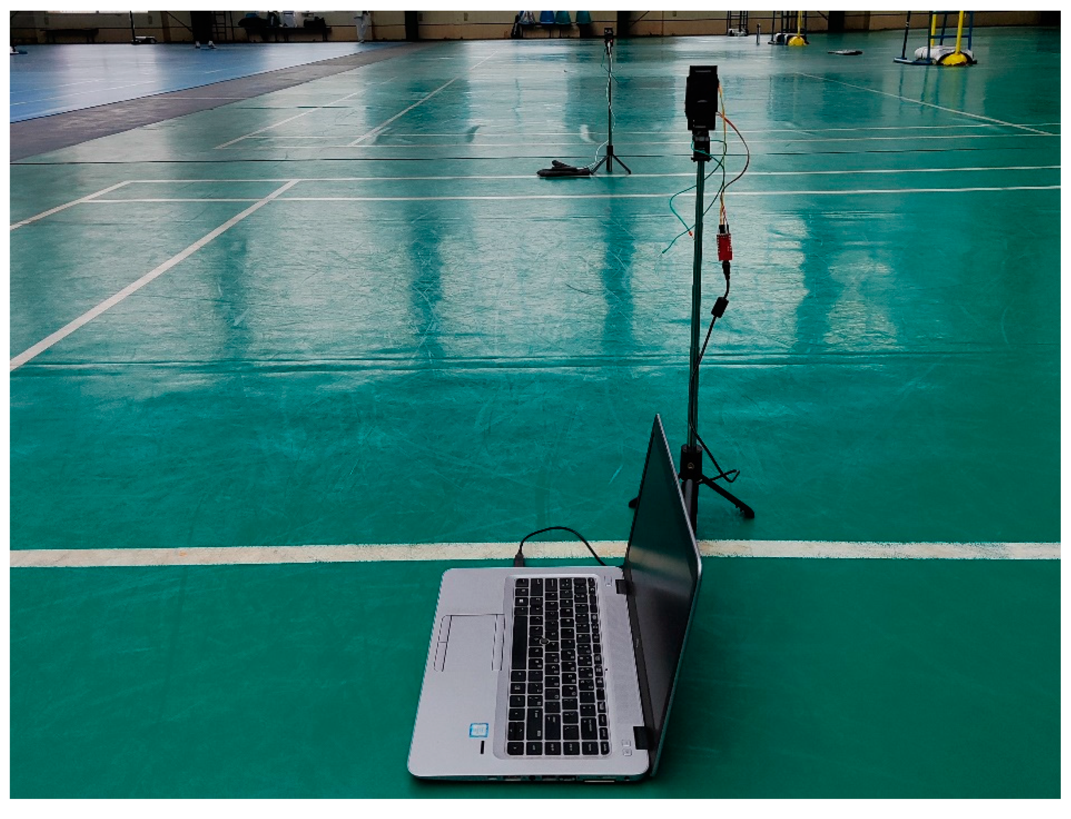
Table 2 presents the results from employing our proposed method for mitigating UWB range errors in an indoor ground environment. The experimental scenario can be seen in Figure 4. Initially, at a baseline distance of 300 cm, the uncorrected measured distance between two UWB devices stood at 268.097 cm. Post-application of our mitigation technique, the distance measured adjusted to 295.177 cm, more closely aligning with the actual distance and resulting in an RMSE of 4.823 cm. Notably, as the baseline distance expanded to 400 cm and then to 500 cm, the effectiveness of our technique in reducing RMSE became increasingly evident, dropping to 2.444 cm and 0.153 cm, respectively. These results not only underscore the significant impact of environmental factors and measurement noise on initial UWB distance measurements but also demonstrate the substantial precision improvements introduced by our mitigation method across various distances. Consequently, this method proves to be highly effective for correcting range measurements, significantly enhancing the accuracy of UWB devices under diverse conditions and at extended ranges, offering promising implications for its application in precision-critical UWB applications.

Table 2. Summary of indoor ground environmental impact on our proposed model showing measured, mitigated, and RMSE errors.

Environment	Original (cm)	Measured (cm)	Mitigated (cm)	RMSE (cm)
	300	268.097	295.177	4.823
Indoor Ground	400	376.866	402.444	2.444
	500	481.257	499.847	0.153

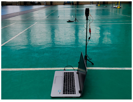
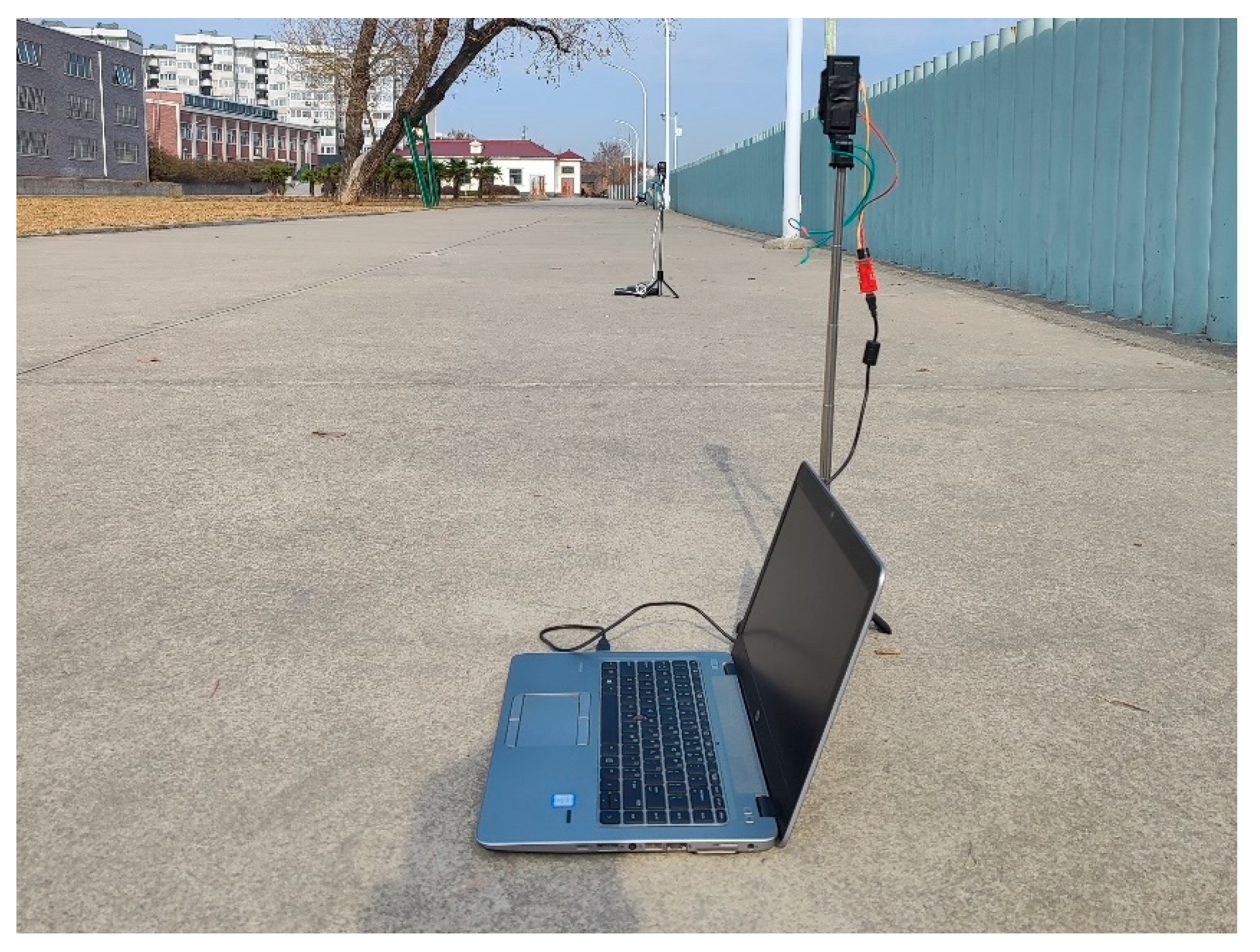
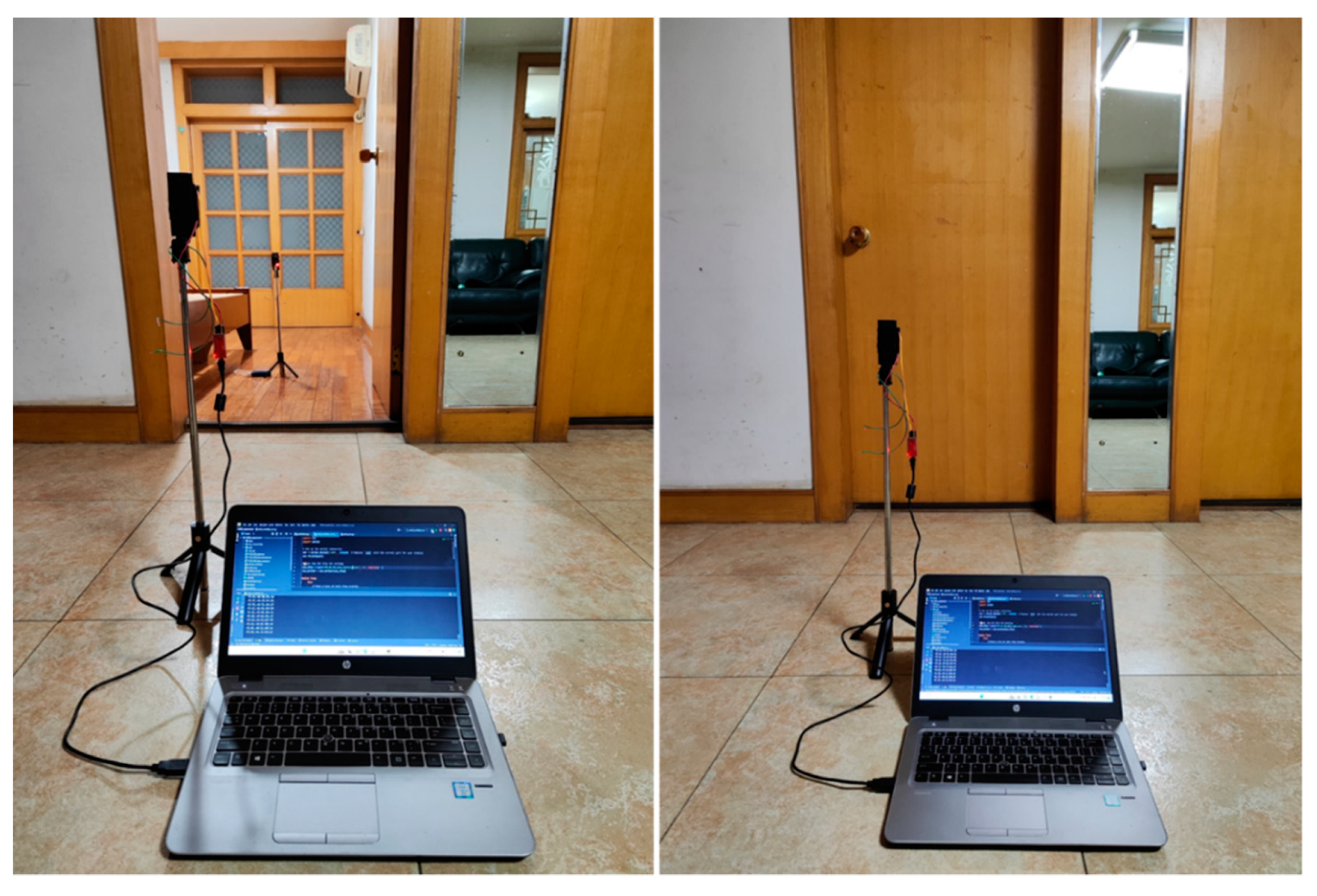
Figure 4. Experiment with line of sight for indoor ground environment.

Table 3 shows the results of applying our proposed method to address UWB range errors under lab conditions. The detailed scenario is shown in Figure 5. Initially, for a 300 cm baseline distance, the uncorrected distance recorded between two UWB devices was 285.510 cm. Following the error mitigation process, this value was refined to 296.796 cm, achieving an RMSE of 3.204 cm. As the baseline distance was extended to 400 cm and 500 cm, the precision of our proposed method was further highlighted. RMSE values were observed to decrease to 3.063 cm and 1.895 cm, respectively, showcasing a consistent improvement in accuracy across increasing distances. Thus, our methodology emerges as a robust solution for refining range measurements, significantly improving the accuracy of UWB devices in lab settings.

Table 3. Summary of lab environmental impact on our proposed model showing measured, mitigated, and RMSE errors.

Environment	Original (cm)	Measured (cm)	Mitigated (cm)	RMSE
	300	285.510	296.796	3.204
Lab	400	389.976	403.063	3.063
	500	492.287	501.895	1.895

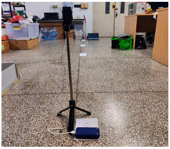
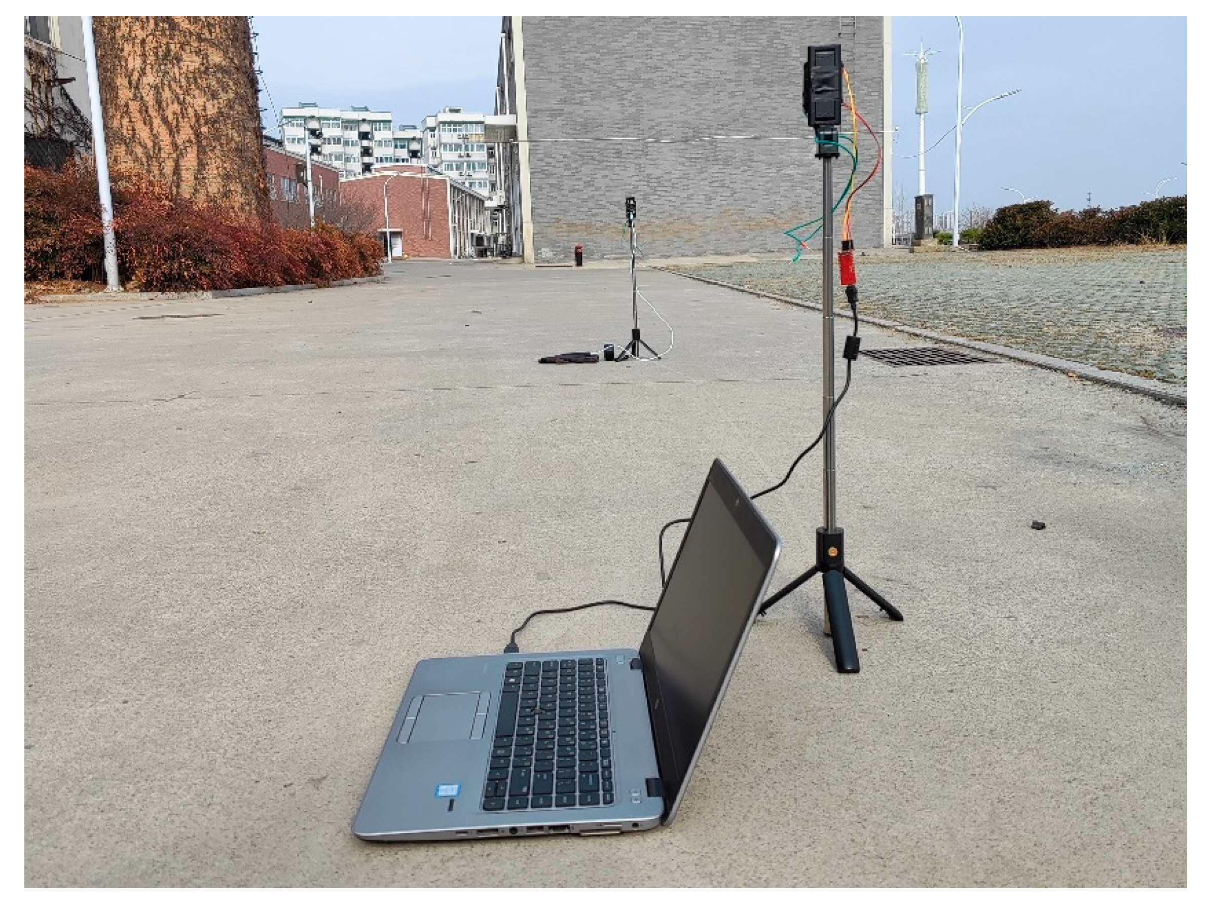
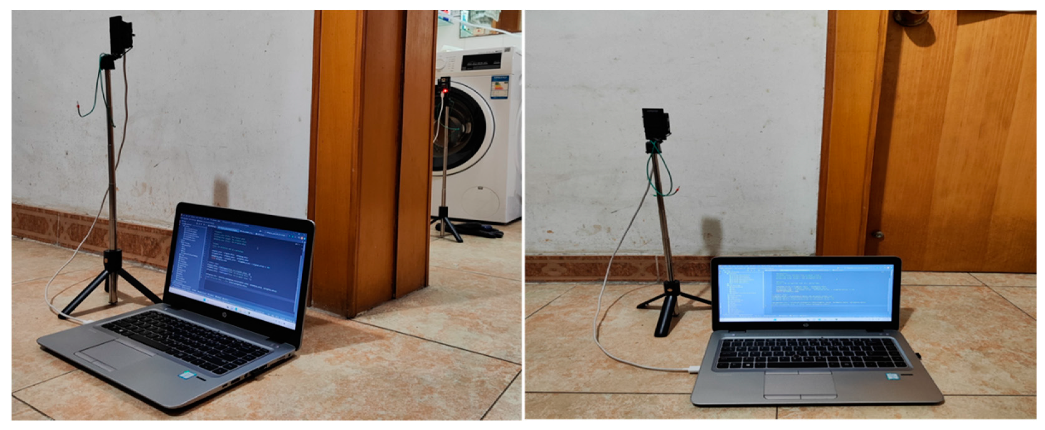
Figure 5. Experiment with line of sight for lab environment.

The data presented in Table 4 illustrate the application of our proposed method for UWB range errors in Park A, across three baseline distances. At 300 cm, the original distance measured was 263.110 cm. After applying the mitigation process, the error was significantly reduced, achieving an RMSE of 2.999 cm. The experimental scenario is given in Figure 6. However, as the distance increased to 400 cm and 500 cm, the RMSE values increased to 6.674 cm and 7.041 cm, respectively. These results suggest that while the mitigation technique is capable of substantially reducing range errors at shorter distances, its efficacy is less pronounced at longer ranges, possibly due to environmental factors specific to Park A. Despite these challenges, the technique demonstrates a significant improvement in UWB measurement accuracy, especially in outdoor environments where precision is critical.

Table 4. Summary of Park A’s environmental impact on our proposed model showing measured, mitigated, and RMSE errors.

Environment	Original (cm)	Measured (cm)	Mitigated (cm)	RMSE
	300	263.110	297.001	2.999
Park A	400	382.083	406.674	6.674
	500	498.694	507.041	7.041

Figure 6. Experiment with line of sight for Park A environment.

Table 5 showcases the effectiveness of a calibration and mitigation approach tailored for ultra-wideband (UWB) range measurements in Park B, encompassing three distinct baseline distances. The detailed scenario is shown in Figure 7. At the initial distance of 300 cm, the original measurement was recorded at 256.612 cm, with the estimated value post-calibration reaching 293.415 cm. Following the mitigation process, an RMSE of 6.585 cm was observed, indicating a notable improvement in accuracy, albeit with some remaining discrepancies. As the distance extended to 400 cm and further to 500 cm, the mitigation technique demonstrated increased efficacy, with RMSEs decreasing to 4.601 cm and 1.487 cm, respectively. This pattern suggests a significant enhancement in the precision of UWB devices with distance, particularly after calibration and mitigation. The decreasing trend in RMSE with longer distances highlights the potential of the applied methodology to effectively address range errors, especially in outdoor settings like Park B, where environmental variables can impact measurement accuracy. Consequently, this approach evidences considerable promise for refining UWB range measurements, ensuring higher accuracy and reliability across varied distances in outdoor environments.

Table 5. Summary of Park B’s environmental impact on our proposed model showing measured, mitigated, and RMSE errors.

Environment	Original (cm)	Measured (cm)	Mitigated (cm)	RMSE
	300	256.612	293.415	6.585
Park B	400	362.322	395.399	4.601
	500	463.113	498.513	1.487

Figure 7. Experiment with line of sight for Park B environment.

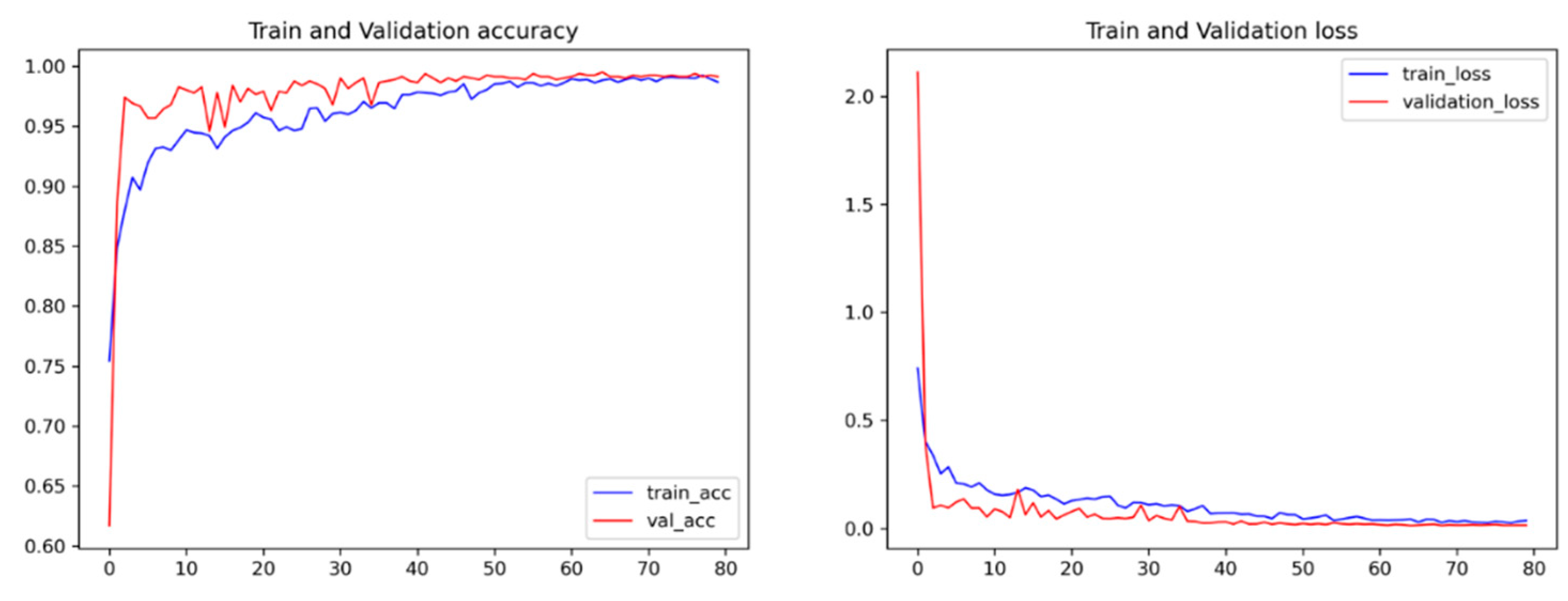
Figure 8 shows the training and validation plot for the accuracy and loss of NLOS identification, respectively. It can be seen that the proposed model converges well with the acquired dataset. The accuracy and loss were stable after 60 epochs and achieved a training accuracy of 99.14% and a validation accuracy of 98.78%.

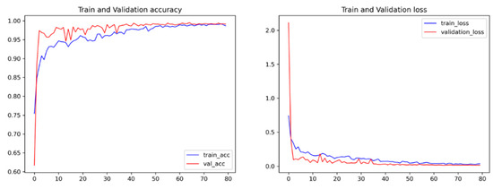
Figure 8. The training and validation accuracy of the proposed model, along with their losses.

We utilized standard multiclass classification evaluation metrics to evaluate the proposed model. In each classification test, we computed the true positive (TP, accurate detection), true negative (TN, correct rejection), false negative (FN, omission error), and false positive (FP, commission error). Using the given formula in [30], we obtained the average classification accuracy (A), average recall (R), average precision (P), and F-1 score (F). Different machine learning methods were implemented on the dataset to evaluate the performance of the proposed model using the following metrics:

$$A={\displaystyle \frac{TP+TN}{TP+TN+FP+FN}}$$

(35)

$$R={\displaystyle \frac{TP}{TP+FN}}$$

(36)

$$P={\displaystyle \frac{TP}{TP+FP}}$$

(37)

$$F=2\ast {\displaystyle \frac{R\ast P}{R+P}}$$

(38)

Table 6 shows the proposed model’s precision, recall, and F-1 score in classifying different NLOS environments. The precision for all classes is 99 or above except for the wood, where the precision is calculated to be 92.1. The model achieves good recall for all the classes, where two classes acquired 99 and one class acquired 100. However, the F-1 score of the proposed model also achieved 100 for the wall and pedestrian environments and 96 for the wood and partial metal environments. The average accuracy achieved from the testing was 98.78.

Table 6. Performance evaluation metrics of the proposed model for each class.

Class Name	Precision	Recall	F-1 Score	Accuracy
Wall	100.0	99.2	100.0	98.78
Partial metal	99.0	94.5	96.3
Wood	92.1	100.0	96.0
Pedestrian	100.0	99.0	100.0

Figure 9 shows the accuracy comparison of various machine learning models for NLOS classification, including LSTM, Conv + LSTM, CNN, CNN + CRFz, random forest, XGBoost, LightGBM, support vector machine (SVM), Naïve Bayes, decision trees, MLP, and the proposed model. The proposed model achieved the highest accuracy of 98.78%, significantly outperforming CNN + CRF (95.87%), LSTM (95.41%), and other models like LightGBM (94.24%), SVM (94.81%), decision trees (93.18%), XGBoost (92.88%), and random forest (91.53%). These results highlight the robustness of the proposed approach in effectively capturing features and adapting to challenging NLOS environments.

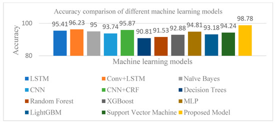
Figure 9. The comparison of different models for NLOS identification in UWB devices.

Table 7 shows the performance of the proposed model with different attention mechanisms, along with their accuracy and processing time. The baseline model, without any attention, achieved an accuracy of 96.32% and a processing time of 5.0 ms per sample. Adding Squeeze-and-Excitation (SE) Attention slightly improved the accuracy to 96.34%, with the processing time increasing to 6.2 ms. Self-Attention, on the other hand, resulted in a lower accuracy of 95.12% and a higher processing time of 9.5 ms, as it was not well suited for the data. Multi-head Attention improved the accuracy to 96.83%, with a processing time of 12.0 ms, by capturing diverse features more effectively.

Table 7. Performance comparison of our proposed model with different attention combinations.

Model	Accuracy	Processing Time
Baseline model	96.32	5.0
Baseline model + SE Attention	96.34	6.2
Baseline model + Self-Attention	95.12	9.5
Baseline model + Multi-head Attention	96.83	12.0
Baseline model + spatial–temporal attention	98.78	15.8

The best performance was achieved with our proposed spatial–temporal attention, which reached an accuracy of 98.78% by extracting both spatial and temporal information. While its processing time was the highest at 15.8 ms per sample, the significant improvement in accuracy makes it worth the trade-off.

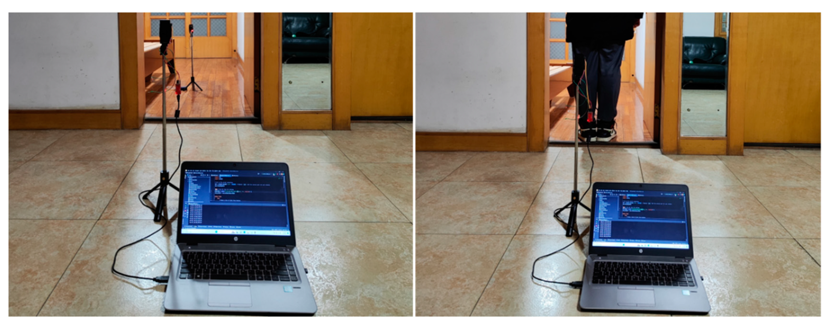
Figure 10 presents an analysis of our proposed system’s accuracy on human obstacles, wherein we compared original distances with measured and mitigated values across three scenarios: 300 cm, 400 cm, and 500 cm. Table 8 presents our findings, showing close approximations of actual distances and effective error correction, as indicated by RMSE values of 6.533, 7.856, and 5.899, respectively. These results highlight the system’s precision and reliability in real-world NLOS scenarios.

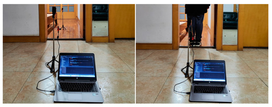
Figure 10. Experiment with non-line-of-sight conditions with human obstacle.

Table 8. Summary of human obstacle’s impact on our proposed model showing measured, mitigated, and RMSE errors.

Obstacle	Original (cm)	Measured (cm)	Mitigated (cm)	RMSE
	300	243.183	293.467	6.533
Human	400	339.414	395.144	4.856
	500	452.802	494.101	5.899

Figure 11 shows the system’s NLOS mitigation accuracy through a comparison of original, measured, and mitigated distances for wood obstacles with various ranges such as 300 cm, 400 cm, and 500 cm. Table 9 illustrates the system’s proficiency in estimating the distance of obstacles with a high degree of accuracy, as demonstrated by the close alignment of measured distances with the original. The mitigation process effectively reduces measurement errors, achieving RMSE values of 8.967, 4.176 for the wood piece, and 4.084 for the largest obstacle. These results emphasize the system’s effectiveness and reliability in diverse detection scenarios.

Figure 11. Experiment with non-line-of-sight conditions with wood obstacle.

Table 9. Summary of wood obstacle’s impact on our proposed model showing measured, mitigated, and RMSE errors.

Obstacle	Original (cm)	Measured (cm)	Mitigated (cm)	RMSE
	300	248.913	296.033	3.967
Wood	400	359.549	395.824	4.176
	500	450.282	495.916	4.084

Figure 12 shows our proposed system's performance on partial metal obstacles, wherein we compared original, measured, and mitigated distances across various ranges. The data reveal the system’s precision in closely approximating the true distances of obstacles, with the measured and mitigated values illustrating the system’s adeptness at error correction. Notably, the RMSE values of 6.986 for a 300 cm partial metal obstacle, 5.894 for a 400 cm partial metal object, and 4.634 for a 500 cm obstacle highlight the system’s consistent accuracy and reliability in a range of scenarios, confirming its effectiveness in real-world applications. The detailed results can be seen in Table 10.

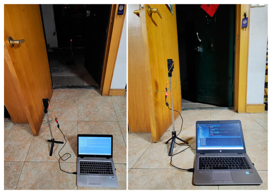
Figure 12. Experiment with non-line-of-sight conditions with partial metal obstacle.

Table 10. Summary of partial metal obstacle’s impact on our proposed model showing measured, mitigated, and RMSE errors.

Obstacle	Original (cm)	Measured (cm)	Mitigated (cm)	RMSE
	300	235.914	293.014	6.986
Partial metal	400	345.278	394.106	5.894
	500	439.492	495.366	4.634

Figure 13 demonstrates the system’s proficiency in detecting obstacles, showcasing a comparison between original, measured, and mitigated distances for a series of obstacles, with a focus on a wall at 400 cm. This comparison clearly illustrates the system’s ability to accurately guess distances, with mitigated measurements closely mirroring the original ones. The RMSE values of 5.935 for the 300 cm wall obstacle, 7.579 for the 400 cm wall obstacle, and 4.195 for the 500 cm wall obstacle shown in Table 11 underscore the system’s precise error correction capabilities across various sizes of obstacles. These findings affirm the system’s robustness and accuracy in obstacle detection within diverse environments.

Figure 13. Experiment with non-line-of-sight conditions with wall obstacle.

Table 11. Summary of wall obstacle’s impact on our proposed model showing measured, mitigated, and RMSE errors.

Obstacle	Original (cm)	Measured (cm)	Mitigated (cm)	RMSE
	300	256.324	294.065	5.935
Wall	400	363.507	393.421	6.579
	500	462.064	495.805	4.195

5.3. Uncertainty Estimation

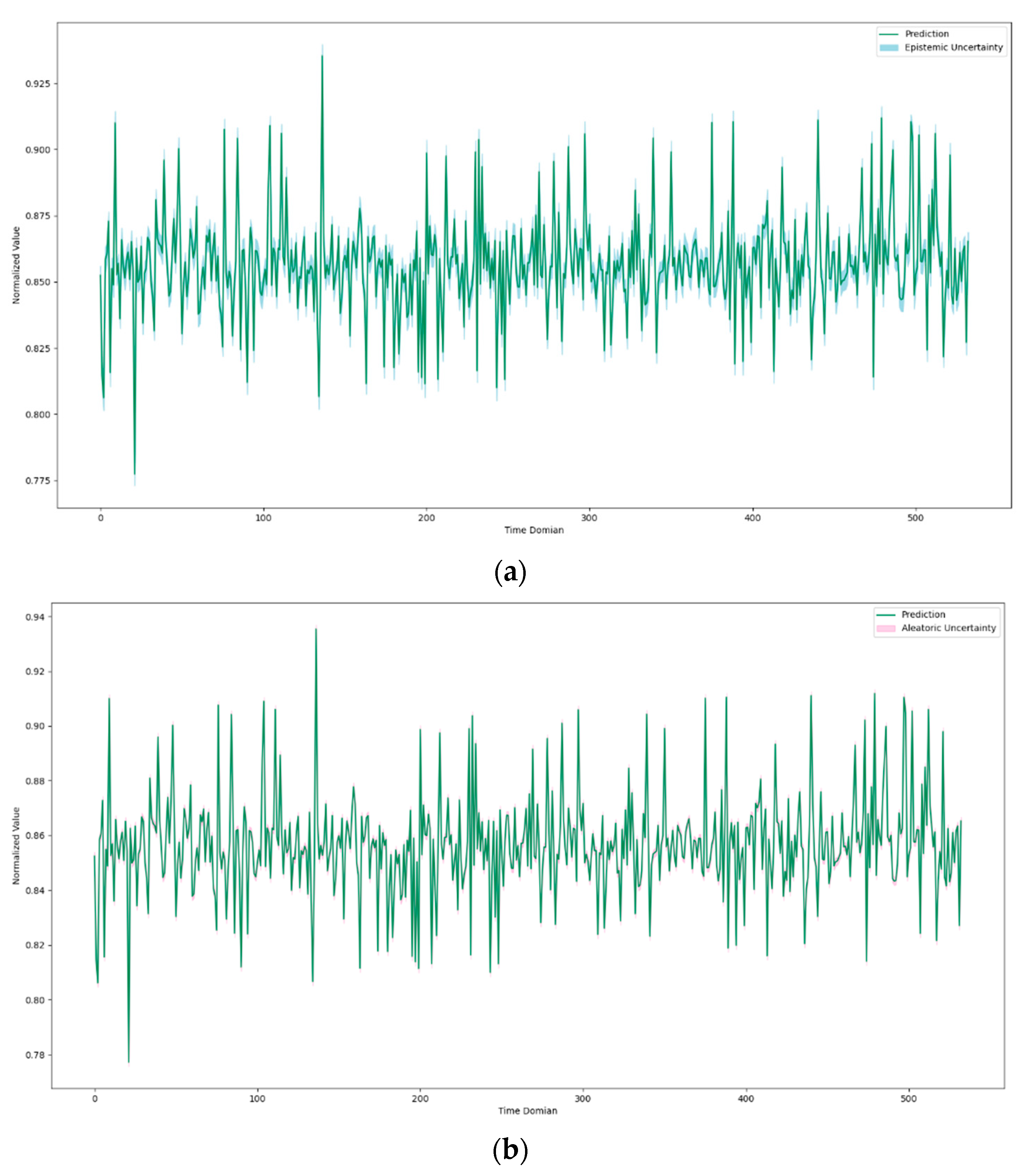
This study utilized the MC dropout method to train the model with variational inference and also calculated the epistemic and aleatoric uncertainty. Different dropout rates were used and tested to determine the best dropout rates for the proposed model. It was observed that the higher dropout rates reduced the accuracy but yielded better model diversity, and the lower dropout rates increased the accuracy but yielded lower model diversity. We found that our proposed model’s dropout rate of 0.50 was optimal; therefore, the dropout rate of 0.50 was used throughout the whole training and experimental procedures. The proposed model’s epistemic uncertainty and aleatoric uncertainty can be found in Figure 14. Figure 14a represents the epistemic uncertainty over the prediction one class. The ideal uncertainty would be very close or identical to the prediction of the relevant class. However, we found that epistemic uncertainty is still present in the prediction process. As stated earlier, epistemic uncertainty represents the lack of data during training, which can be minimized by providing more training data. A mean epistemic uncertainty of 0.00408 was calculated for the proposed model, which was very low. Figure 14b represents the aleatoric uncertainty, which was calculated using the proposed model. It can be seen that the aleatoric uncertainty is very low compared to the epistemic uncertainty. Therefore, it can be said that the inherent noise of the data was smaller, and model performance can be improved by providing more data. A mean aleatoric uncertainty of 0.00534 was calculated for the proposed model, which demonstrates that the aleatoric uncertainty is very low for the acquired dataset and robust to environment variance.

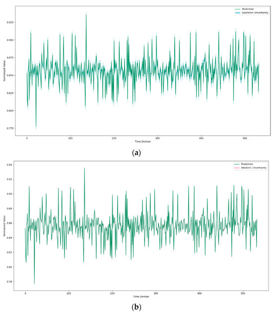
Figure 14. Uncertainty estimation plots with respect to the proposed model’s prediction; (a) the epistemic uncertainty of the proposed model, (b) the aleatoric uncertainty or inherent noise of data calculated using the proposed model.

5.4. Discussion

The proposed NLOS identification is also compared with the different NLOS identification solutions that exist in the literature. Two evaluation metrics are utilized to compare the proposed NLOS identification method with other methods. Yu et al. proposed a fuzzy comprehensive evaluation (FCE)-based method to provide NLOS identification and mitigation solutions [14]. They achieved an accuracy of 96.41% with a recall of 93.90% in identifying NLOS scenarios using UWB devices. Jiang et al. proposed a CNN-based method to identify the NLOS environment for UWB devices [31]. They found that a CNN cascaded with the stacked LSTM method, which achieved a higher accuracy of 82.14%, can provide better accuracy than the LSTM method. Dong et al. proposed Fresnel zones and simple prior knowledge-based methods to provide NLOS identification and mitigation methods for UWB devices [32]. Their proposed method achieved recall and accuracy of 100.00% and 96.41% in identifying the NLOS environment. Cui et al. utilized capsule networks (CapsNet) to classify LOS and NLOS scenarios for UWB-based positioning systems [33]. Their method achieved an accuracy of 94.63% with a 94.74 recall rate. Cung et al. utilized different machine learning methods to identify NLOS conditions in UWB localization, and they achieved a higher overall accuracy of 91.9% using the random forest algorithm [27]. Liu et al. proposed a CNN-GRU-based indoor NLOS/LOS identification neural network to identify the NLOS scenario in an indoor environment [34]. Their proposed method can reach up to 97% accuracy in identifying NLOS and LOS channel propagation in an indoor environment. Musa et al. utilized decision tree machine learning algorithms to detect and mitigate NLOS channel propagation for UWB-based indoor tracking [35]. They tested their model for different NLOS scenarios and achieved an average accuracy of 90.13% with a 91.33% recall rate. Table 12 shows the comparison of the different NLOS identification methods with the proposed method. Our proposed method achieved an accuracy of 98.78% with a 98.17% recall rate. Therefore, it can be said that the proposed method can accurately identify different NLOS scenarios for UWB devices.

Table 12. The comparison of NLOS identification accuracy between different available solutions found in the literature and our proposed method.

Method	Recall	Accuracy
FCE [14]	93.90	96.41
CNN-Stack LSTM [31]	-	82.14
Fresnel zones–prior knowledge [32]	100	82
CapsNet [33]	94.74	94.63
Random forest [27]	-	91.9
CNN-GRU [34]	-	97
Decision tree [35]	91.33	90.13
Proposed	98.17	98.78

We have also compared the mitigated range accuracy with the available NLOS mitigation methods found in the literature to evaluate the performance of our proposed method, as detailed in Table 13. Simone et al. proposed a representation learning model (REMnet) to mitigate NLOS range error prior to positioning using UWB devices. Their method produced a significant improvement in the NLOS range error mitigation, with a mean absolute error of 5.71 cm [30]. Dong et al. proposed NLOS mitigation using the Fresnel zones–prior knowledge method, achieving an accuracy of 10.778 cm in the NLOS environment [32]. Another approach, which uses subdivided NLOS data combined with MIPL-B, achieved a mitigated error of 5.57 cm [36]. A method that involves NLOS/LOS identification followed by error correction reported an error reduction to 10.00 cm [37]. Additionally, a self-supervised deep learning range correction (DLRC) technique showed an improvement, with a mitigated error of 14.681 cm [38]. Barral et al. utilized various machine learning algorithms to identify and mitigate the UWB range measurement in an NLOS environment, achieving the highest reported accuracy of less than 20 cm [39]. Our proposed method has demonstrated a significant reduction in the NLOS effect in UWB-based range measurements, achieving a mean error of 5.30 cm. Based on these results, it can be concluded that our proposed method is effective and can be implemented in real-time UWB range measurement devices to reduce the NLOS effect in range measurements.

Table 13. The comparison of NLOS mitigated accuracy between different available solutions found in the literature and our proposed method.

Method	NLOS Mitigated Error (cm)
REMnet [30]	5.71
Fresnel zones–prior knowledge [32]	10.778
Subdivided NLOS data + MIPL-B [36]	5.57
NLOS/LOS identification + error correction [37]	10.00
Self-supervised DLRC [38]	14.681
Bayesian filter [40]	0.74 (wood), 7.21 (metal)
Machine learning [39]	<20
Proposed	5.30

A potential limitation of the proposed model lies in the increased computational complexity introduced by the spatial–temporal attention mechanism, which may affect its feasibility for deployment on very-low-power devices. Additionally, attention mechanisms may introduce biases by overemphasizing specific features while potentially neglecting others, especially in datasets with imbalanced distributions or high noise levels. To address these challenges, optimization techniques such as model pruning and quantization can be applied to reduce computational demands. Furthermore, we can introduce regularization techniques, and training on diverse and well-balanced datasets can help mitigate biases and improve generalization across various scenarios. We can also explore antenna design, such as a compact triband implantable antenna with superior size, bandwidth, and SAR values, and a 5G wideband MIMO antenna for body-centric networks with high isolation and stable on-body performance to enhance wireless communication in biomedical and body area network applications, which can complement the proposed model’s adaptability in real-world scenarios [41,42].

6. Conclusions

This paper proposes machine learning-based LOS and NLOS identification and mitigation methods to reduce range measurement error in both scenarios. A GP-enhanced non-linear filter is proposed to mitigate the bias of LOS range measurement. The standard deviation of the range measurement for both LOS and NLOS scenarios is mitigated using the min-max removal and the moving average filter. In addition, the NLOS identification method is proposed using the RSSI signal acquired from the UWB range measurement. The Conv-BLSTM method is utilized to identify four common obstacles that can be found in the indoor environment, such as wood, metal, pedestrians, and concrete walls. A spatial–temporal attention module is proposed to improve the performance of the model. Moreover, the uncertainty estimation method is introduced into the proposed model to calculate the epistemic and aleatoric uncertainty. The direct mitigation method is proposed to mitigate the range bias caused by NLOS channel propagation. An extensive experiment was performed to evaluate the performance of the proposed system. The proposed system achieved an accuracy of 3.75 cm in the LOS environment and 5.30 cm in the NLOS environment, with 98.78% NLOS channel propagation identification accuracy.

Our proposed model demonstrates strong potential for real-world applications, such as real-time NLOS classification in autonomous systems and indoor navigation. However, practical deployment may face challenges, including hardware constraints on low-power devices and the need for adaptability to diverse environmental conditions. In the future, we would like to focus on optimizing the model for computational efficiency and validating its performance across varied real-world scenarios to enhance its practicality and robustness. Additionally, we plan to explore other deep learning-based methods, such as graph neural networks and transformer-based architectures to further enhance the feature extraction and improve the model’s performance in challenging scenarios. The effect of room temperature and voltage on the UWB range measurements can be explored to acquire more information on the LOS and NLOS range bias.

References

- Zafari, F.; Gkelias, A.; Leung, K.K. A survey of indoor localization systems and technologies. IEEE Commun. Surv. Tutor. 2019, 21, 2568–2599. [Google Scholar] [CrossRef]
- Asaad, S.M.; Potrus, M.Y.; Ghafoor, K.Z.; Maghdid, H.S.; Mulahuwaish, A. Improving positioning accuracy using optimization approaches: A survey, research challenges and future perspectives. Wirel. Pers. Commun. 2021, 122, 3393–3409. [Google Scholar] [CrossRef]
- Cheng, B.; Cui, L.; Jia, W.; Zhao, W.; Gerhard, P.H. Multiple region of interest coverage in camera sensor networks for tele-intensive care units. IEEE Trans. Ind. Inform. 2016, 12, 2331–2341. [Google Scholar] [CrossRef]
- Zorn, S.; Rose, R.; Goetz, A.; Weigel, R. A novel technique for mobile phone localization for search and rescue applications. In Proceedings of the 2010 International Conference on Indoor Positioning and Indoor Navigation, Zurich, Switzerland, 15–17 September 2010; pp. 1–4. [Google Scholar]
- Jo, K.; Chu, K.; Sunwoo, M. GPS-bias correction for precise localization of autonomous vehicles. In Proceedings of the 2013 IEEE Intelligent Vehicles Symposium (IV), Gold Coast, Australia, 23–26 June 2013; pp. 636–641. [Google Scholar]
- Stahlke, M.; Kram, S.; Mutschler, C.; Mahr, T. NLOS detection using UWB channel impulse responses and convolutional neural networks. In Proceedings of the 2020 International Conference on Localization and GNSS (ICL-GNSS), Tampere, Finland, 2–4 June 2020; pp. 1–6. [Google Scholar]
- Wen, W.W.; Zhang, G.; Hsu, L.T. GNSS NLOS exclusion based on dynamic object detection using LiDAR point cloud. IEEE Trans. Intell. Transp. Syst. 2019, 22, 853–862. [Google Scholar] [CrossRef]
- Gezici, S.; Tian, Z.; Giannakis, G.B.; Kobayashi, H.; Molisch, A.F.; Poor, H.V.; Sahinoglu, Z. Localization via ultra-wideband radios: A look at positioning aspects for future sensor networks. IEEE Signal Process. Mag. 2005, 22, 70–84. [Google Scholar] [CrossRef]
- Fontana, R.J. Recent system applications of short-pulse ultra-wideband (UWB) technology. IEEE Trans. Microw. Theory Technol. 2004, 52, 2087–2104. [Google Scholar] [CrossRef]
- Alarifi, A.; Al-Salman, A.; Alsaleh, M.; Alnafessah, A.; Al-Hadhrami, S.; Al-Ammar, M.A.; Al-Khalifa, H.S. Ultra wideband indoor positioning technologies: Analysis and recent advances. Sensors 2016, 16, 707. [Google Scholar] [CrossRef]
- D‘Amico, A.A.; Mengali, U.; Taponecco, L. Cramer-Rao bound for clock drift in UWB ranging systems. IEEE Wirel. Commun. Lett. 2013, 2, 591–594. [Google Scholar] [CrossRef]
- DecaWave Ltd. DW1000 User Manual. Available online: https://thetoolchain.com/mirror/dw1000/dw1000_user_manual_v2.05.pdf (accessed on 24 March 2024).
- De Angelis, A.; Nilsson, J.; Skog, I.; Peter, H.; Carbone, P. Indoor positioning by ultrawide band radio aided inertial navigation. Metrol. Meas. Syst. 2010, 17, 447–460. [Google Scholar] [CrossRef]
- Yu, K.; Wen, K.; Li, Y.; Zhang, S.; Zhang, K. A novel NLOS mitigation algorithm for UWB localization in harsh indoor environments. IEEE Trans. Veh. Technol. 2018, 68, 686–699. [Google Scholar] [CrossRef]
- Fofana, N.I.; Van den Bossche, A.; Dalcé, R.; Val, T. An original correction method for indoor ultra wide band ranging-based localisation system. In Ad-Hoc, Mobile, and Wireless Networks, Proceedings of the 15th International Conference, ADHOC-NOW 2016, Lille, France, 4–6 July 2016; Proceedings 15; Springer International Publishing: Berlin/Heidelberg, Germany, 2016; pp. 79–92. [Google Scholar]
- Van den Bossche, A.; Dalce, R.; Fofana, I.; Val, T. DecaDuino: An open framework for Wireless Time-of-Flight ranging systems. In Proceedings of the 2016 Wireless Days (WD), Toulouse, France, 23–25 March 2016; pp. 1–7. [Google Scholar]
- Molina Martel, F.; Sidorenko, J.; Bodensteiner, C.; Arens, M. Augmented reality and UWB technology fusion: Localization of objects with head mounted displays. In Proceedings of the 31st International Technical Meeting of the Satellite Division of the Institute of Navigation (ION GNSS+ 2018), Miami, FL, USA, 24–28 September 2018; pp. 685–692. [Google Scholar]
- Dotlic, I.; Connell, A.; McLaughlin, M. Ranging methods utilizing carrier frequency offset estimation. In Proceedings of the 2018 15th Workshop on Positioning, Navigation and Communications (WPNC), Bremen, Germany, 25–26 October 2018; pp. 1–6. [Google Scholar]
- Zhang, Q.; Zhao, D.; Zuo, S.; Zhang, T.; Ma, D. A low complexity NLOS error mitigation method in UWB localization. In Proceedings of the 2015 IEEE/CIC International Conference on Communications in China (ICCC), Shenzhen, China, 2–4 November 2015; pp. 1–5. [Google Scholar]
- Schroeder, J.; Galler, S.; Kyamakya, K.; Jobmann, K. NLOS detection algorithms for ultra-wideband localization. In Proceedings of the 2007 4th Workshop on Positioning, Navigation and Communication, Hannover, Germany, 22 March 2007; pp. 159–166. [Google Scholar]
- Borras, J.; Hatrack, P.; Mandayam, N.B. Decision theoretic framework for NLOS identification. In Proceedings of the VTC’98: 48th IEEE Vehicular Technology Conference. Pathway to Global Wireless Revolution (Cat. No. 98CH36151), Ottawa, ON, Canada, 21 May 1998; Volume 2, pp. 1583–1587. [Google Scholar]
- Lakhzouri, A.; Lohan, E.S.; Hamila, R.; Renfors, M. Extended Kalman filter channel estimation for line-of-sight detection in WCDMA mobile positioning. EURASIP J. Adv. Signal Process. 2003, 2003, 514932. [Google Scholar] [CrossRef]
- Shi, X.; Chew, Y.H.; Yuen, C.; Yang, Z. A RSS-EKF localization method using HMM-based LOS/NLOS channel identification. In Proceedings of the 2014 IEEE International Conference on Communications (ICC), Sydney, Australia, 10–14 June 2014; pp. 160–165. [Google Scholar]
- Casas, R.; Marco, A.; Guerrero, J.J.; Falco, J. Robust estimator for non-line-of-sight error mitigation in indoor localization. EURASIP J. Adv. Signal Process. 2006, 2006, 043429. [Google Scholar] [CrossRef]
- Wymeersch, H.; Maranò, S.; Gifford, W.M.; Win, M.Z. A machine learning approach to ranging error mitigation for UWB localization. IEEE Trans. Commun. 2012, 60, 1719–1728. [Google Scholar] [CrossRef]
- Van Nguyen, T.; Jeong, Y.; Shin, H.; Win, M.Z. Machine learning for wideband localization. IEEE J. Sel. Areas Commun. 2015, 33, 1357–1380. [Google Scholar] [CrossRef]
- Sang, C.L.; Steinhagen, B.; Homburg, J.D.; Adams, M.; Hesse, M.; Rückert, U. Identification of NLOS and multi-path conditions in UWB localization using machine learning methods. Appl. Sci. 2020, 10, 3980. [Google Scholar] [CrossRef]
- Tian, Q.; Kevin, I.; Wang, K.; Salcic, Z. Human body shadowing effect on UWB-based ranging system for pedestrian tracking. IEEE Trans. Instrum. Meas. 2018, 68, 4028–4037. [Google Scholar] [CrossRef]
- Gal, Y.; Ghahramani, Z. Dropout as a bayesian approximation: Representing model uncertainty in deep learning. In Proceedings of the Proceedings of the 33rd International Conference on International Conference on Machine Learning, New York, NY, USA, 19–24 June 2016; pp. 1050–1059.
- Angarano, S.; Mazzia, V.; Salvetti, F.; Fantin, G.; Chiaberge, M. Robust ultra-wideband range error mitigation with deep learning at the edge. Eng. Appl. Artif. Intell. 2021, 102, 104278. [Google Scholar] [CrossRef]
- Jiang, C.; Shen, J.; Chen, S.; Chen, Y.; Liu, D.; Bo, Y. UWB NLOS/LOS classification using deep learning method. IEEE Commun. Lett. 2020, 24, 2226–2230. [Google Scholar] [CrossRef]
- Dong, M. A low-cost NLOS identification and mitigation method for UWB ranging in static and dynamic environments. IEEE Commun. Lett. 2021, 25, 2420–2424. [Google Scholar] [CrossRef]
- Cui, Z.; Liu, T.; Tian, S.; Xu, R.; Cheng, J. Non-line-of-sight identification for UWB positioning using capsule networks. IEEE Commun. Lett. 2020, 24, 2187–2190. [Google Scholar] [CrossRef]
- Liu, Q.; Yin, Z.; Zhao, Y.; Wu, Z.; Wu, M. UWB LOS/NLOS identification in multiple indoor environments using deep learning methods. Phys. Commun. 2022, 52, 101695. [Google Scholar] [CrossRef]
- Musa, A.; Nugraha, G.D.; Han, H.; Choi, D.; Seo, S.; Kim, J. A decision tree-based NLOS detection method for the UWB indoor location tracking accuracy improvement. Int. J. Commun. Syst. 2019, 32, e3997. [Google Scholar] [CrossRef]
- Deng, B.; Xu, T.; Yan, M. UWB NLOS Identification and Mitigation Based on Gramian Angular Field and Parallel Deep Learning Model. IEEE Sens. J. 2023, 23, 28513–28525. [Google Scholar] [CrossRef]
- Yang, H.; Wang, Y.; Seow, C.K.; Sun, M.; Si, M.; Huang, L. UWB sensor-based indoor LOS/NLOS localization with support vector machine learning. IEEE Sens. J. 2023, 23, 2988–3004. [Google Scholar] [CrossRef]
- Yang, B.; Li, J.; Shao, Z.; Zhang, H. Self-supervised deep location and ranging error correction for UWB localization. IEEE Sens. J. 2023, 23, 9549–9559. [Google Scholar] [CrossRef]
- Barral, V.; Escudero, C.J.; García-Naya, J.A.; Maneiro-Catoira, R. NLOS identification and mitigation using low-cost UWB devices. Sensors 2019, 19, 3464. [Google Scholar] [CrossRef]
- Xin, J.; Gao, K.; Shan, M.; Yan, B.; Liu, D. A Bayesian filtering approach for error mitigation in ultra-wideband ranging. Sensors 2019, 19, 440. [Google Scholar] [CrossRef]
- Gupta, A.; Kumar, V.; Bansal, S.; Alsharif, M.H.; Jahid, A.; Cho, H.-S. A Miniaturized Tri-Band Implantable Antenna for ISM/WMTS/Lower UWB/Wi-Fi Frequencies. Sensors 2023, 23, 6989. [Google Scholar] [CrossRef]
- Gupta, A.; Kumari, M.; Sharma, M.; Alsharif, M.H.; Uthansakul, P.; Uthansakul, M.; Bansal, S. 8-port MIMO Antenna at 27 GHz for n261 Band and Exploring for Body Centric Communication. PLoS ONE 2024, 19, e0305524. [Google Scholar] [CrossRef]
Disclaimer/Publisher’s Note: The statements, opinions and data contained in all publications are solely those of the individual author(s) and contributor(s) and not of MDPI and/or the editor(s). MDPI and/or the editor(s) disclaim responsibility for any injury to people or property resulting from any ideas, methods, instructions or products referred to in the content. |
© 2024 by the authors. Licensee MDPI, Basel, Switzerland. This article is an open access article distributed under the terms and conditions of the Creative Commons Attribution (CC BY) license (https://creativecommons.org/licenses/by/4.0/).